Entanglement entropy scaling in solid-state spin arrays via capacitance measurements

Abstract

Solid-state spin arrays are being engineered in varied systems, including gated coupled quantum dots and interacting dopants in semiconductor structures. Beyond quantum computation, these arrays are useful integrated analog simulators for many-body models. As entanglement between individual spins is extremely short ranged in these models, one has to measure the entanglement entropy of a block in order to truly verify their many-body entangled nature. Remarkably, the characteristic scaling of entanglement entropy, predicted by conformal field theory, has never been measured. Here we show that with as few as two replicas of a spin array, and capacitive double-dot singlet-triplet measurements on neighboring spin pairs, the above scaling of the entanglement entropy can be verified. This opens up the controlled simulation of quantum field theories, as we exemplify with uniform chains and Kondo-type impurity models, in engineered solid-state systems. Our procedure remains effective even in the presence of typical imperfections of realistic quantum devices and can be used for thermometry, and to bound entanglement and discord in mixed many-body states.

Introduction.–  More than two decades of active research in quantum information processing has promoted various quantum technologies, which are believed to result in a new industrial revolution Dowling and Milburn (2003). One of the major goals, which dates back to Feynmann Feynman (1982), is to simulate complex interacting quantum systems, which are intractable with classical computers, with an engineered and controllable quantum device, the so-called quantum simulator Cirac and Zoller (2012). Unlike general-purpose quantum computers, which are supposed to be programmable to achieve different tasks, quantum simulators are designed for a specific goal, which make them easier to realize. Indeed, so far cold atoms Bloch et al. (2012) and ions Blatt and Roos (2012) have been used for successfully simulating certain tasks. Nevertheless, solid state based quantum simulator is still highly in demand due to the fact that: i) they provide more versatile types of interaction and stronger couplings compared to cold atoms and ions; ii) the quest towards miniaturization in electronics has reached the quantum level, making solid state quantum devices feasible Salfi et al. (2016).

Much theoretical researches have been conducted to understand the highly entangled structures appearing in the ground state of quantum many-body systems Amico et al. (2008). For a given bipartition $A$ and $B$ of the whole system, which is assumed to be in the pure state $\rho_{AB}{=}|{\psi_{AB}}\rangle\langle{\psi_{AB}}|$, the entanglement entropy is quantified by $S_{\alpha}(\rho_{A}){=}S_{\alpha}(\rho_{B})$, where $\rho_{A}{=}\operatorname*{Tr}_{B}\rho_{AB}$ and $S_{\alpha}$ is the Renyi entropy, defined as

$$S_{\alpha}(\rho)=\frac{1}{1-\alpha}\log\operatorname*{Tr}[\rho^{\alpha}]~{},$$ (1)

for different values of $\alpha$. When $\alpha{\to}1$ the Renyi entropy reduces to the von Neumann entropy $S_{1}(\rho){=}{-}\operatorname*{Tr}[\rho\log\rho]$. The importance of the entanglement entropy is twofold: i) it quantifies the entanglement between $A$ and $B$; ii) the discovery of its area law dependence in non-critical systems has immensely contributed to the development of efficient approximation techniques Eisert et al. (2010) for describing many-body systems. On the other hand, in critical one-dimensional systems with open boundary conditions, conformal field theory analysis shows that there is a logarithmic correction, as

$$S_{\alpha}(x)=\frac{c}{12}\left(1+\frac{1}{\alpha}\right)\log\left[\frac{2N}{\pi}\sin\left(\frac{\pi x}{N}\right)\right]+\kappa_{\alpha}$$ (2)

where $x$ is the size of the contiguous block $A$ starting at one end of system, and $N$ is the total size. When $N{\gg}x{\gg}1$ the usual scaling $S_{\alpha}{\propto}\log x$ is obtained. This formula is very general and the central charge $c$ only depends on the universality class of the model, while the constants $\kappa_{\alpha}$ are model dependent Calabrese et al. (2010); Calabrese and Cardy (2004); Fagotti and Calabrese (2011).

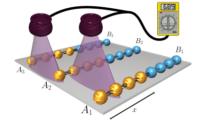
Figure 1: Scheme for the measurement of the Entanglement entropy for $\alpha{=}3$ using three copies of the same spin chain. Each spin chain is divided into $A_{i}$ (yellow spins) and $B_{i}$ (blue spins). By performing sequential singlet-triplet measurements of pair of spins in neighbouring chains is it possible to estimate $S_{\alpha{=}3}(\rho_{A})$ (see the discussion in the text), which measures the entanglement between $A$ and $B$.

In spite of the extensive theoretical literature on entanglement entropy, its experimental measurement is a big challenge. For itinerant bosonic particles it has been proposed Alves and Jaksch (2004); Daley et al. (2012), and recently realized Kaufman et al. (2016), to use beam splitter operations or discrete Fourier transform to measure $S_{\alpha}$. Alternatively measuring entropy through quantum shot noise has been proposed Song et al. (2012); Klich and Levitov (2009), but not yet realized. On the other hand, in non-itinerant spin systems, the situation become even more difficult and the only proposal so far is to use spin-dependent switches Abanin and Demler (2012), which are difficult to build.

Here we put forward a proposal for measuring $S_{\alpha}$ in a spin system without demanding time-dependent particle delocalition or spin-dependent switches. While our setup can be realized in different physical systems, we target it to solid state systems, such as gated quantum dot chains Loss and DiVincenzo (1998); Hanson et al. (2007); Baart et al. (2016); Nakajima et al. (2016); Ito et al. (2016); Zajac et al. (2016); Noiri et al. (2016) or dopant arrays Kane (1998); Zwanenburg et al. (2013); Salfi et al. (2016); Fuechsle and Simmons (2013). Our procedure is based on well established singlet-triplet measurements, which are now routinely performed either via charge detection Petta et al. (2005) or capacitive radio-frequency reflectometry House et al. (2015); Petersson et al. (2010); Frey et al. (2012); Colless et al. (2013).

Measuring entanglement entropy.–  Our goal is to measure $S_{\alpha}$ for arbitrarily integer values of $\alpha{\geq}2$. For simplicity we explain the procedure for $\alpha{=}2$ and then generalize it for higher values. Inspired by previous alternative proposals Horodecki and Ekert (2002); Alves and Jaksch (2004); Daley et al. (2012); Abanin and Demler (2012); Cardy (2011) we make use of two copies of a spin array in the state $\rho_{1}{\otimes}\rho_{2}$ (ideally for perfect copies $\rho_{1}{=}\rho_{2}$). Each copy is identically divided into two complementary blocks: $A_{1}$ and $B_{1}$ for the first copy, $A_{2}$ and $B_{2}$ for the second one (see Fig. 1). Let $x$ be the number of spins in $A_{1}$ (and $A_{2}$). We define the multi-spin swap operator acting on $A_{1}$ and $A_{2}$ as

$$P_{12}^{A}{\equiv}\bigotimes_{\ell=1}^{x}{\rm SWAP}({\ell_{A_{1}},\ell_{A_{2}}}),$$ (3)

where ${\rm SWAP}({\ell_{A_{1}},\ell_{A_{2}}})$ swaps the two spins at the $\ell$-th sites in $A_{1}$ and $A_{2}$. Since all the operators ${\rm SWAP}({\ell_{A_{1}},\ell_{A_{2}}})$ are commuting it is simple to show that

$$\langle{P_{12}^{A}}\rangle=\operatorname*{Tr}[P_{12}^{A}\,\rho_{1}{\otimes}\rho_{2}]=\operatorname*{Tr}[\rho_{A_{1}}\rho_{A_{2}}]=\operatorname*{Tr}[\rho_{A}^{2}]$$ (4)

where the last equality holds if the two copies are identical, namely $\rho_{A_{1}}{\equiv}\rho_{A_{2}}{\equiv}\rho_{A}$. Therefore, Eq. (4) implies that $S_{2}{=}{-}\log\langle{P_{12}^{A}}\rangle$ can be obtained via a sequential measurement of pairwise swap operators acting on the different spins of $A_{1}$ and $A_{2}$, as shown in Fig. 1.

The above procedure can be generalized to higher integer values of $\alpha$ by considering $\alpha$ copies of the spin array in the state $\rho^{\otimes\alpha}{=}\bigotimes_{\ell{=}1}^{\alpha}\rho_{\ell}$ (where ideally all the $\rho_{\ell}$’s are equal). Remarkably sequential measurements of multi-spin swap operators acting on neighboring copies $a$ and $a{+}1$, namely $P^{A}_{a,a{+}1}$, is sufficient to measure the Renyi entropy. This is simple, but not trivial as better explained in the Appendix A, because some $P^{A}_{(a,a{+}1)}$’s for different $a$ are non-commuting. However, we show that the simple sequential measurement, exemplified also in Fig. 1, corresponds to the measurement of the operator $P^{(A)}_{12\dots\alpha}$ which is defined recursively by the formula

$$P^{A}_{12\dots\alpha}=\frac{P^{A}_{\alpha,\alpha{-}1}P^{A}_{1\dots\alpha{-}1}+P^{A}_{1\dots\alpha{-}1}P^{A}_{\alpha,\alpha{-}1}}{2}.$$ (5)

For example for $\alpha{=}3$ this reduces to $P^{A}_{123}{=}(P^{A}_{23}P^{A}_{12}{+}P^{A}_{12}P^{A}_{23})/2$ and $\langle{P^{A}_{123}}\rangle{=}(\operatorname*{Tr}[\rho_{A_{1}}\rho_{A_{2}}\rho_{A_{3}}]{+}\operatorname*{Tr}[\rho_{A_{1}}\rho_{A_{3}}\rho_{A_{2}}])/2$, so that for perfect copies $\langle{P^{A}_{123}}\rangle{=}\operatorname*{Tr}[\rho_{A}^{3}]$. In general using Eq. (1) we have $S_{\alpha}(\rho_{A}){=}(1{-}\alpha)^{-1}\log\langle{P^{A}_{12\dots\alpha}}\rangle$. We stress that $P^{A}_{12\dots\alpha}$ is ultimately written in terms nearest neighbor multi-spin swap operators $P^{A}_{(a,a{+}1)}$. This makes the procedure scalable in the lab as one has to first measure $P^{A}_{12}$, then $P^{A}_{23}$ and so forth till $P^{A}_{\alpha{-}1,\alpha}$.

Solid state spin chains.–  When exactly one electron is trapped in each quantum dot, the interactions between confined electrons in quantum dot arrays is restricted to the spin sector, and is described by the Heisenberg Hamiltonian

$$H=\sum_{k=1}^{N-1}J_{k}\boldsymbol{\sigma}_{k}\cdot\boldsymbol{\sigma}_{k+1},$$ (6)

where $J_{k}$ is the exchange coupling between neighboring sites and $\boldsymbol{\sigma}_{k}{=}(\sigma^{x}_{k},\sigma^{y}_{k},\sigma^{z}_{k})$ is the vector of Pauli operators acting on site $k$. The couplings $J_{k}$ can be locally tuned by appropriately changing the local gate voltages. The system can be initialized into its ground state either by cooling, when temperatures is below its energy gap, or using an adiabatic-type evolution Farooq et al. (2015) when temperature is higher.

Singlet-triplet measurements on two electrons trapped in adjacent quantum dots is now a well-established technique for spin measurements in solid state physics Petta et al. (2005); Petersson et al. (2010); Frey et al. (2012); Colless et al. (2013); Delbecq et al. (2016). In a quantum mechanical language the singlet-triplet measurements on a pair of electrons in dots $a$ and $b$ correspond to projective measurements of the swap operator, as one can show

$${\rm SWAP}(a,b)=\sum_{\mu=\pm,0}|{t_{\mu}}\rangle\langle{t_{\mu}}|-|{s}\rangle\langle{s}|=\frac{\openone+\boldsymbol{\sigma}_{a}\cdot\boldsymbol{\sigma}_{b}}{2},$$ (7)

$|{s}\rangle{=}(|{{\uparrow}_{a}{\downarrow}_{b}}\rangle{-}|{{\downarrow}_{a}{\uparrow}_{b}}\rangle)/\sqrt{2}$ is the singlet state, and $|{t_{+}}\rangle{=}|{{\uparrow}_{a}{\uparrow}_{b}}\rangle$, $|{t_{0}}\rangle{=}(|{{\uparrow}_{a}{\downarrow}_{b}}\rangle{+}|{{\downarrow}_{a}{\uparrow}_{b}}\rangle)/\sqrt{2}$, $|{t_{-}}\rangle{=}|{{\downarrow}_{a}{\downarrow}_{b}}\rangle$ are the triplet states. The outcome of this measurement is either $+1$, for triplet outcomes, and $-1$ for the singlet one.

By comparing Eqs. (7) and (3) it is now clear that, for any given bipartition, we can use a sequence of singlet-triplet measurements to obtain the outcome of the operators $P^{A}_{1\dots\alpha}$ and thus compute all the Renyi entropies $S_{\alpha}$ for all integer $\alpha{\geq}2$. As described before, and shown also in Fig. 1, the total number of singlet-triplet measurements to be performed for a single outcome is $x\alpha$ where $x$ is the number of spins in subsystem $A$. To measure $P^{A}_{1\dots\alpha}$ we first switch off the $J_{k}$’s within each array, and then lower the barriers between pairs of spins in two different arrays to perform the singlet-triplet measurements. A recently developed multiplexer structure Puddy et al. (2015) containing two parallel arrays of quantum dots is a promising setup, which can be adapted for measuring $S_{2}$ with our proposed mechanism. Motivated by this operating device, and for the sake of simplicity, in the rest of the paper we focus on $\alpha{=}2$. Numerical results are obtained with either Density Matrix Renormalization Group (DMRG) or exact diagonalization for short chains.

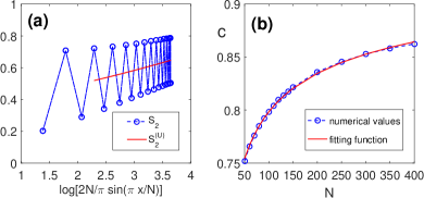
Figure 2: (color online) (a) Scaling of $S_{2}$ and its uniform part $S^{(U)}_{2}$ in terms of differet sizes of block $A$, for a chain of $N{=}60$. (b) Scaling of the central charge $c$ as a function of length $N$.

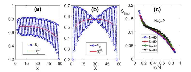
Figure 3: (color online) (a) The Renyi entropy $S_{2}(x,N,\xi)$ and its uniform part $S_{2}^{(U)}$ in a chain of length $N{=}60$. (b) The bulk Renyi entropy $S_{2}(x{-}1,N{-}1)$ and its uniform part $S_{2}^{(U)}(x{-}1,N{-}1)$ in a homogeneous chain of 59 sites without impurity. (c) Data collapse for different chains when $J^{\prime}$ is tuned to keep $N/\xi{=}2$.

Application 1: conformal field theory in the lab.–  We first present how field theory predictions, given in Eq. (2), can be verified for a uniform chain where $J_{k}{=}J$, for all $k$’s. In the thermodynamic limit $N{\to}\infty$ it is known that the central charge is $c{=}1$. In Fig. 2(a) we plot the Renyi entropy $S_{2}$ as a function of $\log[\frac{2N}{\pi}\sin(\frac{\pi x}{N})]$ in a chain of length $N=60$. For open boundary conditions, finite size effects are known Calabrese et al. (2010) to give rise to an alternating behaviour of $S_{2}(x){=}S_{2}^{(U)}{+}({-}1)^{x}S_{2}^{(A)}$. Using the methodology of Ref. Sørensen et al. (2007) we extract the uniform part $S_{2}^{(U)}$, which is dominant for $N{\to}\infty$ and follows the scaling of (2). In Fig. 2(a) we also plot $S_{2}^{(U)}$ in red colors, showing perfect linear scaling. From the slope of this line we can extract the central charge $c$, which asymptocically approaches its thermodynamic limit value, $c{=}1$. This can be seen in Fig. 2(b) where we also plot the fitting function $c=1-0.7536N^{-0.2848}$. Such slow convergence is due to finite-size corrections to the field theory predictions Xavier and Alcaraz (2012), which here, for simplicitly, we have absorbed into the definition of $c$.

Application 2: impurity entanglement entropy.–  Introducing one or more impurities in the system can change its behaviour drammatiacaly. A paradigmatic example is the single-impurity Kondo model Affleck (2008) in which a single impurity in a gapless system creates a length scale $\xi$, known as Kondo length. The scaling features of Kondo physics can be captured by a spin chain emulation of this model Sørensen et al. (2007). This is described by Eq. (6) where $J_{1}{=}J^{\prime}$ while all other couplings remain uniform $J_{k}{=}J$ (for $k{\geq}2$). Moreover, the length scale is determined by $J^{\prime}$ as $\xi{\propto}e^{{g}/J^{\prime}}$ for some constant $g$. The presence of the impurity modifies the scaling of the Eq. (2) when $x{<}\xi$. In order to capture the impurity contribution of the entanglement entropy we extend the ansatz of Ref. Sørensen et al. (2007) for $S_{1}$ to generic $S_{\alpha}$ and define the impurity entanglement entropy as

$$S_{\alpha}^{(imp)}(x,N,\xi)=S_{\alpha}^{(U)}(x,N,\xi)-S_{\alpha}^{(U)}(x-1,N-1),$$ (8)

where $S_{\alpha}^{(U)}(x,N,\xi)$ is the Renyi entropy of a block of size $x$ in a chain of length $N$ and impurity coupling $J^{\prime}$, which determines $\xi$, while $S_{\alpha}^{(U)}(x{-}1,N{-}1)$ represents the bulk contribution of the uniform chain when the impurity is removed. In Fig. 3(a) we plot the $S_{2}(x,N,\xi)$ and its uniform part $S_{2}^{(U)}$ in a chain of length $N=60$. The bulk contribution of the uniform chain, i.e. $S_{2}(x{-}1,N{-}1)$, and its uniform part $S_{2}^{(U)}(x{-}1,N{-}1)$ are plotted in Fig. 3(b). The qualitative difference between Fig. 3(a) and Fig. 3(b) is due to the different parities (i.e. even and odd) of the chains.

The emergence of the length scale implies that $S_{2}^{(imp)}(x,N,\xi)$ is only a function of the ratios $S_{2}^{(imp)}(x/N,N/\xi)$. To verify this scaling we fix $N/\xi$ and plot $S_{2}^{(imp)}$ as a function of $x/N$ for different lengths $N$. To keep $N/\xi$ fixed $J^{\prime}$ has to be tuned according to Ref. Bayat et al. (2010). The results are shown in Fig. 3(c) where, as predicted, the curves of different chains collapse oneach other. Although the data collapse becomes better by increasing the system size, Fig. 3(c) shows that the scaling predictions can be captured even in relatively small chains.

Application 3: entanglement spectrum.–  For any pure state $\rho_{AB}$ the eigenvalues of $\rho_{A}$ are called entanglement spectrum Li and Haldane (2008), whose analysis is important to characterize quantum phase transitions De Chiara et al. (2012); Bayat et al. (2014). The eigenvalues of $\rho_{A}$ are the roots of $q(\lambda){=}\det(\lambda\openone{-}\rho_{A})$, which can be written as $q(\lambda){=}\sum_{k}g_{k}\lambda^{k}$. According to Ref. Curtright and Fairlie (2012) the coefficients $g_{k}$ can be obtained algorithmically from $\operatorname*{Tr}[\rho_{A}^{\alpha}]$ for $\alpha{=}1,\dots,k$. Since these traces can be measured with our procedure one can build $q(\lambda)$ and hence obtain the full entanglement spectrum. Clearly, given a maximum number of copies $\alpha_{\rm max}$, one can find the entanglement spectrum for block sizes as large as $x{=}\log_{2}\alpha_{\rm max}$.

Application 4: thermometry via purity measurement.–  One of the biggest challenges in solid-state experiments is to measure the true temperature of electrons, as it is normally higher than the temperature of the refrigerator. Remarkably, our scheme enables also to measure the electronic temperature via singlet-triplet measurements, assuming that the system is in a thermal state $\rho_{\beta}{=}e^{{-}\beta H}/Z$. Our approach is based on three distinctive features of engineered solid state structures: i) the exchange integral $J$ can be varied; ii) the purity $\mathcal{P}(\beta,J){=}\operatorname*{Tr}[\rho_{\beta}^{2}]{=}e^{{-}S_{2}(\rho_{\beta})}$ can be measured with our scheme by taking two copies and $x{=}N$; iii) computing the energy expectation $E(\beta,J){=}\operatorname*{Tr}[H\rho_{\beta}]$ is reduced to singlet-triplet measurements on neighboring sites of one of the arrays, thanks to Eqs. (7) and (6). A simple calculation reveals that $\frac{\partial\mathcal{P}(\beta,J)}{\partial J}{=}\frac{\beta}{J}[2E(\beta,J){-}E(\beta,2J)]\mathcal{P}(\beta,J)$. Aside from $\beta$ all the quantities in the above equality can be measured either directly (namely $\mathcal{P}(\beta,J)$ and $E(\beta,J)$) or through the variation of $J$ (namely $\frac{\partial\mathcal{P}(\beta,J)}{\partial J}$ and $E(\beta,2J)$). In summary, thanks to the above equality, using different singlet-triplet measurements with different values of $J$ it is possible to infer $\beta$ and thus the temperature.

Application 5: bounding entanglement and discord in mixed states.–  The Renyi entropy of a block $A$ is a measure of entanglement between $A$ and $B$ only if $\rho_{AB}$ is a pure state. However, we show that it is still possible to bound the amount of entanglement and discord also for mixed states by measuring both $S_{\alpha}(\rho_{A})$ and $S_{\alpha}(\rho_{AB})$. The distillable entanglement $E_{D}$, an operational entanglement measure, satisfies the hashing inequality Devetak and Winter (2005), $E_{D}{\geq}\max_{X{=}A,B}I_{1}(X)$, where $I_{1}(X){=}S_{1}(\rho_{X}){-}S_{1}(\rho_{AB})$. Similarly, for the quantum discord $D(A|B)$, which is an asymmetric measure of quantum correlations between $A$ and $B$ Ollivier and Zurek (2001), it is known that $D(A|B){\geq}I_{1}(A)$ and similarly $D(B|A){\geq}I_{1}(B)$ Fanchini et al. (2011). The von Neumann entropy $S_{1}$ can be extrapolated De Nobili et al. (2015) from $S_{\alpha}$ for different integers $\alpha{\geq}2$, which can be measured with our scheme. However, we show that $I_{1}$ can also be bounded by directly measuring $S_{2}(\rho_{A})$ and $S_{2}(\rho_{AB})$, which require only two replicas. Indeed, since $S_{2}(\rho){\leq}S_{1}(\rho){\leq}f[S_{2}(\rho)]$, where $f$ is given in Ref. Życzkowski (2003), we obtain $I_{1}(X){\geq}I_{2}(X)$ where $I_{2}(X){=}S_{2}(\rho_{X})-f[S_{2}(\rho_{AB})]$. For either $X{=}A,B$, $I_{2}(X)$ thus provides a measureble lower bound to entanglement and discord.

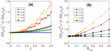
Figure 4: (color online) (a) Average $\mathbb{E}[S_{2}(\rho^{\{\delta\}}_{A})]$ over 1000 random sets of couplings $J^{(j)}_{k}{=}J_{k}(1{+}\epsilon^{(j)}_{k})$, where $j{=}1,2$ refers to the different copies, $J_{k}{=}J$ and $\epsilon^{(j)}_{k}$ is uniformly distributed in $[{-}\delta,{+}\delta]$ for different block sizes $x$ (b) Monte Carlo simulation of $\mathbb{E}[S_{2}(\rho^{\{B_{\rm nuc}\}}_{A})]$ for the effect of random fields $B_{k}^{(j)}$ as a function of the strength of the hyperfine interaction $B_{\rm nuc}$. In both figures the entropies are normalized with respect to the error-free case $S_{2}(\rho_{A})$, and $N{=}10$.

Imperfections.–  Realistic experimental imperfections may introduce errors, e.g. by making the different copies non-identical. Our protocol provides $\operatorname*{Tr}[\rho_{A_{1}}\rho_{A_{2}}]$, as given in Eq. (4), which may deviate from the ideal case $\operatorname*{Tr}[\rho_{A}^{2}]$. Indeed, imperfect fabrication may result in random couplings $J^{(j)}_{k}{\rightarrow}J_{k}(1{+}\epsilon^{(j)}_{k})$, where $j$ is the index of different copies and $\epsilon_{k}^{(j)}$ is a random number uniformly distributed between $[-\delta,+\delta]$. In Fig.4(a) we calculate the average $\mathbb{E}[S_{2}(\rho^{\{\delta\}}_{A})]$ over 1000 random sets of couplings for different block sizes $x$, normalized with respect to its value at $\delta{=}0$. As the figure shows the average entropy increases by increasing $\delta$. Moreover, up to $\delta{=}10\%$ the outcomes are almost indistinguishable from the error-free case.

The second source of imperfections is due to the hyperfine interaction with the nuclear spins in the bulk, which effectively introduces an extra term $\sum_{k}\boldsymbol{B}^{(j)}_{k}\cdot\boldsymbol{\sigma}_{k}$ in the Hamiltonian (6), where each compoenent of the random fields has a normal distribution with zero mean and variance $B_{\rm nuc}$. Unlike the randomness in the couplings, which is constant over different experiments being due to the fabrication, the effective random fields are different in any experimental repeatition. To realistically model this, we perform a Monte Carlo simulation of real experimental outcomes (see the Appendix C for details). The results are shown in Fig. 4(b) for different block sizes $x$. For realistic values of $B_{\rm nuc}{=}0.1J$ Petta et al. (2005) we see that the entanglement entropy is only slightly affected by hyperfine interactions. The increasing trend of the entropy as a function of the noise, which is consistent with Ref. Getelina et al. (2016), is further discussed in the Appendix B.

Conclusions.–  We propose a scheme to expeimentally measure the entanglement between blocks in engineered solid state quantum devices. Our procedure is based on singlet-triplet measurements which are rountinely performed in quantum dot systems. All the Renyi entanglement entropies $S_{\alpha}$ for integer $\alpha{\geq}2$ can be measured via $\alpha$ replicas of the system. Although for uniform chains the convergence of the central charge is slow, the logarithmic scaling predictions can already be verified with reasonably small system sizes ($\lesssim 60$). Moreover, in the Kondo impurity model we found that the impurity contribution in the Renyi entropy satisfies a universal scaling law. Despite the fact this law has been obtained in the thermodynamic limit, remarkably it can be observed for chains as small as $N{\gtrsim}30$. In addition, our scheme enables the measurement of the purity of the whole system, which allows one to measure the true temperature of electrons in a thermal state. Our procedure remains effective even in the presence of typical imperfections due to imperfect fabrication and hyperfine interactions. Although our scheme has been targeted to quantum dot arrays, the same protocol can also be realized in other systems, such as dopants in silicon Zwanenburg et al. (2013).

Appendix A Renyi entropies of arbitrary orders via singlet-triplet measurements

Singlet-triplet (ST) projective measurements can be described by the pair of projection operators $\Pi_{-}{=}|{s}\rangle\langle{s}|$, $\Pi_{+}{=}\sum_{\alpha{=}{-}1}^{1}|{t_{\alpha}}\rangle\langle{t_{\alpha}}|$ where $|{s}\rangle{=}(|{{\uparrow}{\downarrow}}\rangle{-}|{{\downarrow}{\uparrow}}\rangle)/\sqrt{2}$ is the singlet state, and $|{t_{1}}\rangle{=}|{{\uparrow}{\uparrow}}\rangle$, $|{t_{0}}\rangle{=}(|{{\uparrow}{\downarrow}}\rangle{+}|{{\downarrow}{\uparrow}}\rangle)/\sqrt{2}$, $|{t_{-1}}\rangle{=}|{{\downarrow}{\downarrow}}\rangle$ are the triplet states. To relate this measurement with the estimation of the entropy it is convenient to define the swap operator ${\rm SWAP}$ which is related to the ST-measurement via $\Pi_{\pm}{=}(\openone{\pm}{\rm SWAP})/2$. Note that the SWAP operator can be also written in terms of the Heisenberg spin exchange ${\rm SWAP}{\equiv}(\openone{+}\sum_{\alpha{=}{x,y,z}}\sigma_{\alpha}{\otimes}\sigma_{\alpha})/2$, where $\sigma_{\alpha}$ are the Pauli matrices. Since ${\rm SWAP}{=}\Pi_{+}{-}\Pi_{-}$ the ST-measurement can be understood as a projective measurement of the SWAP operator: given a two qubit state, this measurement can result in two different outcomes, either $+1$ or $-1$, with respective probability $\operatorname*{Tr}[\rho\Pi_{\pm}]$.

Our strategy to measure the Renyi entropy $S_{\alpha}(\rho){=}(1{-}\alpha)^{-1}\log\operatorname*{Tr}[\rho^{\alpha}],$ is based on two fundamental observations: (i) as shown in Horodecki and Ekert (2002) if one has access to $m$ copies of the same state $\rho$, then $\operatorname*{Tr}[\rho^{m}]{=}\operatorname*{Tr}[P_{(12\dots m)}\rho^{\otimes m}]$ where $\rho^{\otimes m}{=}\rho{\otimes}\rho{\otimes}{\dots}{\otimes}\rho$ and $P_{(12\dots m)}|{\psi_{1}}\rangle{\otimes}|{\psi_{2}}\rangle\dots|{\psi_{m}}\rangle{=}|{\psi_{m}}\rangle{\otimes}|{\psi_{1}}\rangle\dots|{\psi_{m-1}}\rangle$ is a permutation operator, which swaps different states according to the cyclic permutation $(12\dots m)$; (ii) the operator $P_{(12\dots m)}$ can be decomposed in terms of a series of swap between neighboring copies. In the following we show how to interpret these multiple swap operations in terms of single-triplet measurements, as shown in Fig. 1.

We first focus on the measure of the entanglement entropy for $\alpha{=}2$. This is quite straightforward, but we review this in detail to introduce the necessary formalism and to clarify why this simple analysis cannot be applied for $\alpha{>}2$. We consider two copies of the same system, each divided into two disjoint blocks: the first copy is composed by the blocks $A_{1}$ and $B_{1}$ and the second one by the blocks $A_{2}$ and $B_{2}$. From the previous analysis it is clear that $S_{2}{=}\frac{1}{2}\log\langle{P_{(12)}^{A}}\rangle$, where $P_{(12)}^{A}$ is a multi-spin swap between the spins in $A_{1}$ and those in $A_{2}$. Let $x$ be the number of spins in $A_{1}$ (and $A_{2}$) and let $i_{1}\dots i_{x}$ be the indices of the spin in $A_{1}$, while $j_{1},\dots j_{x}$ are the indices of the spins in $A_{2}$. Blocks $A_{1}$ and $A_{2}$ are non-overlapping. The multi-spin swap then reads $P_{(12)}^{A}{\equiv}\bigotimes_{\ell=1}^{x}{\rm SWAP}_{i_{\ell}j_{\ell}}$ where ${\rm SWAP}_{ij}$ is the swap operator between the pair of spins $(i,j)$. Therefore, in order to measure the expectation value $\langle{P_{(12)}^{A}}\rangle$, one has to perform a series of multiple singlet-triplet measurements between different pairs $(i_{\ell},j_{\ell})$ of spins, and collect the resulting statistics. Indeed, the first projective measurement will result in an outcome $\pm 1$ and a collapse of $\rho_{A_{1}A_{2}B_{1}B_{2}}$ into the (non-normalized) state $\Pi_{\pm}^{(i_{1},j_{1})}\rho_{A_{1}A_{2}B_{1}B_{2}}\Pi_{\pm}^{(i_{1},j_{1})}$, where $\Pi_{\pm}^{(i_{1},j_{1})}$ is the ST projector for the pair $(i_{1},j_{1})$; after the $x$ projective measurements between all pair of spins the outcome will be $(\prod_{\ell{=}1}^{x}\beta_{\ell})1$, where $\beta_{\ell}{=}\pm$, with probability $\operatorname*{Tr}[\rho_{A_{1}A_{2}B_{1}B_{2}}\bigotimes_{\ell{=}1}^{x}\Pi_{\beta_{\ell}}^{(i_{\ell},j_{\ell})}]$. Therefore, running these projections many-times will enable an experimental evaluation of $\langle{P_{(12)}^{A}}\rangle$.

We now consider the case $\alpha{=}3$. For convenience we write $P_{(12)}^{A}{=}\Pi_{(12)}^{+}{-}\Pi^{-}_{(12)}$ in terms of the projection operators (indeed, as shown before also $P_{(12)}^{A}$ has eigenvalues $\pm 1$). We first perform a sequential set of ST-measurements on copies $(1,2)$, with outcome $\beta_{1}$ and then do the same measurement on copies $(2,3)$, with outcome $\beta_{2}$. We introduce the notation $P^{A}_{(23)}\circ P^{A}_{(12)}$ to describe this process. After the first measurement, the (non-normalized) state of the system will be $\Pi_{(12)}^{\beta_{1}}\rho\Pi^{\beta_{1}}_{(12)}$, where $\rho{=}\rho_{1}{\otimes}\rho_{2}{\otimes}\rho_{3}$, while after the two sets of measurements it is $\Pi_{(23)}^{\beta_{2}}\Pi_{(12)}^{\beta_{1}}\rho\Pi^{\beta_{1}}_{(12)}\Pi_{(23)}^{\beta_{2}}$. Therefore,

$$\langle{P^{A}_{(23)}\circ P^{A}_{(12)}}\rangle =\sum_{\beta_{2}}\sum_{\beta_{1}}\beta_{1}\beta_{2}\operatorname*{Tr}\left[\Pi_{(23)}^{\beta_{2}}\Pi_{(12)}^{\beta_{1}}\rho\Pi^{\beta_{1}}_{(12)}\Pi_{(23)}^{\beta_{2}}\right]$$

$$=\sum_{\beta_{2}}\sum_{\beta_{1}}\beta_{1}\beta_{2}\operatorname*{Tr}\left[\Pi^{\beta_{1}}_{(12)}\Pi_{(23)}^{\beta_{2}}\Pi_{(12)}^{\beta_{1}}\rho\right]$$

$$=\sum_{\beta_{1}}\beta_{1}\operatorname*{Tr}\left[\Pi^{\beta_{1}}_{(12)}P_{(23)}^{A}\Pi_{(12)}^{\beta_{1}}\rho\right]$$

$$=\frac{1}{2}\left(\operatorname*{Tr}[P^{A}_{(12)}P_{(23)}^{A}\rho]+\operatorname*{Tr}[P_{(23)}^{A}P_{(12)}^{A}\rho]\right)$$

$$=\frac{1}{2}\left(\operatorname*{Tr}[P^{A}_{(123)}\rho]+\operatorname*{Tr}[P_{(132)}^{A}\rho]\right)$$

$$=\frac{1}{2}\left(\operatorname*{Tr}[\rho_{1}\rho_{2}\rho_{3}]+\operatorname*{Tr}[\rho_{1}\rho_{3}\rho_{2}]\right),$$ (9)

where we used multiple times the fact that $\Pi^{\pm}_{(ab)}{=}(\openone{\pm}{P}^{A}_{(ab)})/2$ and, in the last equation, that $P^{A}_{(123)}$ and $P^{A}_{(132)}$ are permutation operators, and $(123),(132)$ different cycles. The above equation shows that, because of the non-commutative nature of $P_{(12)}^{A}$ and $P_{(23)}^{A}$, the sequential process described in Fig. 1 ends up in the measurement of a combination of different permutation operators.

We now generalize the above argument for higher values of $\alpha$. We apply sequential ST-measurements on neighbouring copies, using the notation $P_{(12)}^{A}{\circ}P_{(23)}^{A}{\circ}{\cdots}{\circ}P_{(\alpha{-}1,\alpha)}^{A}$, meaning that we first perform $P_{(12)}^{A}$ and so forth. As already seen for $\alpha{=}3$, the reason for this notation is that, as we show, $\langle{P_{(12)}^{A}{\circ}P_{(23)}^{A}{\circ}\cdots{\circ}P_{(\alpha{-}1,\alpha)}^{A}}\rangle{\neq}\langle{P_{(12)}^{A}P_{(23)}^{A}\cdots P_{(\alpha{-}1,\alpha)}^{A}}\rangle$. Indeed, after the first measurement of $P_{(12)}^{A}$, with outcome $\beta_{1}{=}\pm$, the (non-normalized) state is $\Pi_{(12)}^{\beta_{1}}\rho_{AB}\Pi_{(12)}^{\beta_{1}}$. At later stages one performs sequentially the other measurements $P_{(j,j{+}1)}^{A}$, getting the outcomes $\beta_{j}$. Taking the averages one then finds that

$$\langle{P_{(\alpha{-}1,\alpha)}^{A}{\circ}{\cdots}{\circ}P_{(12)}^{A}}\rangle{=}\operatorname*{Tr}[\mathcal{P}_{\alpha{-}1,\alpha}[\cdots\mathcal{P}_{23}[\mathcal{P}_{12}[\rho]]]\cdots],$$

where $\mathcal{P}_{j,j{+}1}[\rho]{=}\sum_{\beta_{j}}\beta_{j}\Pi_{(j,j{+}1)}^{\beta_{j}}\rho\Pi_{(j,j{+}1)}^{\beta_{j}}$. Using the cyclic property of the trace and the identity $\mathcal{P}_{j{-}1,j}[P^{A}_{(nab\dots)}]=[P^{A}_{(j{-}1,j,a,\dots)}{+}P^{A}_{(j,j{-}1,a,\dots)}]/2$ multiple times (where $a{>}j$, $b{>}j$ and so forth), one finds that $\langle{P_{(\alpha{-}1,\alpha)}^{A}{\circ}{\cdots}{\circ}P_{(12)}^{A}}\rangle{=}2^{2{-}\alpha}\sum_{c}\langle{P^{A}_{c}}\rangle$ where $c$ are $2^{\alpha{-}2}$ different cycles, namely cyclic permutations of the elements $1,\dots,{\alpha}$. For instance, for $\alpha{=}3$ one has $c{=}\{(123),(132)\}$. From the above expression it turns out that, if the copies are perfect, then the different cycles have the same expectation value $\langle{P^{A}_{c}}\rangle{=}\operatorname*{Tr}[\rho^{\alpha}]$ and therefore

$$S_{\alpha}=\frac{1}{1{-}\alpha}\log\langle{P_{(\alpha{-}1,\alpha)}^{A}{\circ}{\cdots}{\circ}P_{(12)}^{A}}\rangle~{}.$$ (10)

On the other hand, if the different copies are not exactly equal, then there may be an extra error (see the numerical examples in the main text). In Eq.(10) each $P_{(j,j{+}1)}^{A}$ requires $x$ ST-measurements ($x$ being the number of spins in $A_{i}$), so the total number of ST-measurements for a single outcome is $x\alpha$.

Appendix B Imperfections

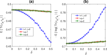
Figure 5: (a) Average purity $\mathbb{E}[\operatorname*{Tr}[\rho_{A_{i}}\rho_{A_{j}}]]$ and (b) average Renyi entropy $\mathbb{E}[{-}\log\operatorname*{Tr}[\rho_{A_{i}}\rho_{A_{j}}]]$ as a function of the noise strength $\delta$, calculated with our strategy (where $i{\neq}j$ and each copy feels a different noise) and with the standard procedure (where $i{=}j$). In all cases $N{=}10$, $x{=}5$.

We compare the role of the imperfections in our protocol and in the standard one in Fig. 5. We consider the noise model discussed in the main text where the couplings $J_{k}$ are different over the different copies, namely $J_{k}^{(j)}{=}J_{k}(1{+}\epsilon_{k}^{(j)})$ where $j$ refers to the index of the copies. The errors $\epsilon_{k}^{(j)}$ are independent identically distributed according to a uniform distribution with zero mean and variance $\delta$. For simplicity we consider only $\alpha{=}2$. In Fig. 5(a) we show that the average purity estimated with our strategy, i.e. $\mathbb{E}[\operatorname*{Tr}[\rho_{A_{1}}\rho_{A_{2}}]]$, is smaller than the one evaluated with the standard procedure on each chain, i.e. $\mathbb{E}[\operatorname*{Tr}[\rho_{A_{1}}^{2}]]$ and $\mathbb{E}[\operatorname*{Tr}[\rho_{A_{2}}^{2}]]$. On the other hand, since the Renyi entropy is minus the logarithm of the purity, the average Renyi entropy displays the opposite behavior, as shown in Fig. 5(b). This can be explained with the following argument. When $\epsilon_{k}^{(j)}{\ll}1$ we can expand the states $\rho_{A_{j}}$ in series of $\epsilon_{k}^{(j)}$ and write

$$\rho_{A_{j}}\simeq\rho_{A}+\sum_{k}\epsilon_{k}^{(j)}\rho^{\prime}_{k}+\sum_{k,\ell}\epsilon_{k}^{(j)}\epsilon_{\ell}^{(j)}\rho^{\prime\prime}_{k,\ell},$$ (11)

where $\rho^{\prime}_{k}$ and $\rho^{\prime\prime}_{k,\ell}$ are the first order and second-order expansion, which are independent on the index $j$. Therefore,

$$\mathbb{E}[\operatorname*{Tr}[\rho_{A_{1}}\rho_{A_{2}}]]\simeq\operatorname*{Tr}[\rho_{A}^{2}]+2\delta^{2}\sum_{k}\operatorname*{Tr}[\rho^{\prime\prime}_{k,k}\rho_{A}]~{},$$ (12)

while

$$\mathbb{E}[\operatorname*{Tr}[\rho_{A_{1}}^{2}]] =\mathbb{E}[\operatorname*{Tr}[\rho_{A_{2}}^{2}]]$$ (13)

$$\simeq\operatorname*{Tr}[\rho_{A}^{2}]+\delta^{2}\sum_{k}\left(2\operatorname*{Tr}[\rho^{\prime\prime}_{k,k}\rho_{A}]+\operatorname*{Tr}[\rho^{\prime}_{k}{}^{2}]\right)~{}.$$

The results of Fig. 5 show that the quantity $\sum_{k}\operatorname*{Tr}[\rho^{\prime\prime}_{k,k}\rho_{A}]$ is negative and lowers the average purity. On the other hand, $\operatorname*{Tr}[\rho^{\prime}_{k}{}^{2}]$ is clearly positive, being the trace of the square of an operator. The latter term then partially removes the effect of the negative one and makes $\mathbb{E}[\operatorname*{Tr}[\rho_{A_{i}}^{2}]]{\approx}\operatorname*{Tr}[\rho_{A}^{2}]$. On the other hand, independent copies are slightly more affected by the uncorrelated noise and $\mathbb{E}[\operatorname*{Tr}[\rho_{A_{1}}\rho_{A_{2}}]]{<}\mathbb{E}[\operatorname*{Tr}[\rho_{A_{i}}^{2}]]{\lesssim}\operatorname*{Tr}[\rho_{A}^{2}]$. The error is nonetheless small, since it is smaller than 10% even for 50% of randomness.

Appendix C Monte Carlo simulation of random fields

As explained in the main text, hyperfine interactions with the nuclear spins result in the couplings $\sum_{k}\boldsymbol{B}_{k}\cdot\boldsymbol{\sigma}$. The random effective fields $\boldsymbol{B}_{k}$ are assumed to be constant after each different ST-measurement required to get a single outcome. However, to get the necessary statistics to estimate (10) one has to repeat the experiment many times. Since each time the system is re-initialized, the corresponding random fields may be different. To study this kind of imperfections we perform the following Monte Carlo simulation

1. We generate the random fields $B^{\alpha}_{k,c}$ for different $\alpha{=}x,y,z$, different sites $k{=}1,\dots,N$ and different copies $c{=}1,\dots,\alpha$ independently according to a Gaussian distribution, with zero mean and variance $\sigma$.

2. We calculate, with exact numerical diagonalization, the quantum mechanical probability

   $$p{=}\sum_{\prod_{j}\beta_{j}={+1}}\operatorname*{Tr}\left[\prod_{j}\Pi^{\beta_{j}}_{(j,j{+}1)}\rho\prod_{l}\Pi^{\beta_{l}}_{(l,l{+}1)}\right],$$

   to get the outcome ${+}1$. In the above equation $\rho{=}\rho_{1}{\otimes}\cdots{\otimes}\rho_{\alpha}$ where $\rho_{j}$ is the ground state of the $j$-th copy with the random fields. In general therefore $\rho_{i}{\neq}\rho_{j}$.

3. We generate a random number q in $[0,1]$. If $q{<}p$ we say that the outcome of the sequence of projective measurements is ${+}1$, otherwise it is ${-}1$.

4. We repeat the steps 1,2,3 $T$ times to estimate $\langle{P_{(\alpha{-}1,\alpha)}^{A}{\circ}{\cdots}{\circ}P_{(12)}^{A}}\rangle$, and then calculate $S_{\alpha}$.

5. We repeat the steps 1,2,3,4 $K$ times to calculate the average $\mathbb{E}[S_{\alpha}]$ and the variance.

In the following figures we show the outcome of this procedure for $N{=}10$, $x{=}1,\dots,N/2$ as a function of $\sigma$, when $K{=}T{=}100$. The red lines correspond to the exact numerical calculation of $S_{\alpha}$ when $\sigma{=}0$.

References

- Dowling and Milburn (2003) J. P. Dowling and G. J. Milburn, Philosophical Transactions of the Royal Society of London A: Mathematical, Physical and Engineering Sciences 361, 1655 (2003).
- Feynman (1982) R. P. Feynman, International journal of theoretical physics 21, 467 (1982).
- Cirac and Zoller (2012) J. I. Cirac and P. Zoller, Nature Physics 8, 264 (2012).
- Bloch et al. (2012) I. Bloch, J. Dalibard, and S. Nascimbene, Nature Physics 8, 267 (2012).
- Blatt and Roos (2012) R. Blatt and C. Roos, Nature Physics 8, 277 (2012).
- Salfi et al. (2016) J. Salfi, J. Mol, R. Rahman, G. Klimeck, M. Simmons, L. Hollenberg, and S. Rogge, Nature communications 7 (2016).
- Amico et al. (2008) L. Amico, R. Fazio, A. Osterloh, and V. Vedral, Reviews of Modern Physics 80, 517 (2008).
- Eisert et al. (2010) J. Eisert, M. Cramer, and M. B. Plenio, Reviews of Modern Physics 82, 277 (2010).
- Calabrese et al. (2010) P. Calabrese, M. Campostrini, F. Essler, and B. Nienhuis, Physical review letters 104, 095701 (2010).
- Calabrese and Cardy (2004) P. Calabrese and J. Cardy, Journal of Statistical Mechanics: Theory and Experiment 2004, P06002 (2004).
- Fagotti and Calabrese (2011) M. Fagotti and P. Calabrese, Journal of Statistical Mechanics: Theory and Experiment 2011, P01017 (2011).
- Alves and Jaksch (2004) C. M. Alves and D. Jaksch, Physical review letters 93, 110501 (2004).
- Daley et al. (2012) A. Daley, H. Pichler, J. Schachenmayer, and P. Zoller, Physical review letters 109, 020505 (2012).
- Kaufman et al. (2016) A. M. Kaufman, M. E. Tai, A. Lukin, M. Rispoli, R. Schittko, P. M. Preiss, and M. Greiner, arXiv preprint arXiv:1603.04409 (2016).
- Song et al. (2012) H. F. Song, S. Rachel, C. Flindt, I. Klich, N. Laflorencie, and K. Le Hur, Physical Review B 85, 035409 (2012).
- Klich and Levitov (2009) I. Klich and L. Levitov, Physical review letters 102, 100502 (2009).
- Abanin and Demler (2012) D. A. Abanin and E. Demler, Physical review letters 109, 020504 (2012).
- Loss and DiVincenzo (1998) D. Loss and D. P. DiVincenzo, Physical Review A 57, 120 (1998).
- Hanson et al. (2007) R. Hanson, L. Kouwenhoven, J. Petta, S. Tarucha, and L. Vandersypen, Reviews of Modern Physics 79, 1217 (2007).
- Baart et al. (2016) T. Baart, N. Jovanovic, C. Reichl, W. Wegscheider, and L. Vandersypen, arXiv preprint arXiv:1606.00292 (2016).
- Nakajima et al. (2016) T. Nakajima, M. R. Delbecq, T. Otsuka, S. Amaha, J. Yoneda, A. Noiri, K. Takeda, G. Allison, A. Ludwig, A. D. Wieck, et al., arXiv preprint arXiv:1604.02232 (2016).
- Ito et al. (2016) T. Ito, T. Otsuka, S. Amaha, M. R. Delbecq, T. Nakajima, J. Yoneda, K. Takeda, G. Allison, A. Noiri, K. Kawasaki, et al., arXiv preprint arXiv:1604.04426 (2016).
- Zajac et al. (2016) D. Zajac, T. Hazard, X. Mi, E. Nielsen, and J. Petta, arXiv preprint arXiv:1607.07025 (2016).
- Noiri et al. (2016) A. Noiri, J. Yoneda, T. Nakajima, T. Otsuka, M. R. Delbecq, K. Takeda, S. Amaha, G. Allison, A. Ludwig, A. D. Wieck, et al., Applied Physics Letters 108, 153101 (2016).
- Kane (1998) B. E. Kane, nature 393, 133 (1998).
- Zwanenburg et al. (2013) F. A. Zwanenburg, A. S. Dzurak, A. Morello, M. Y. Simmons, L. C. Hollenberg, G. Klimeck, S. Rogge, S. N. Coppersmith, and M. A. Eriksson, Reviews of Modern Physics 85, 961 (2013).
- Fuechsle and Simmons (2013) M. Fuechsle and M. Y. Simmons, Single-Atom Nanoelectronics , 61 (2013).
- Petta et al. (2005) J. R. Petta, A. C. Johnson, J. M. Taylor, E. A. Laird, A. Yacoby, M. D. Lukin, C. M. Marcus, M. P. Hanson, and A. C. Gossard, Science 309, 2180 (2005).
- House et al. (2015) M. House, T. Kobayashi, B. Weber, S. Hile, T. Watson, J. van der Heijden, S. Rogge, and M. Simmons, Nature communications 6 (2015).
- Petersson et al. (2010) K. Petersson, C. Smith, D. Anderson, P. Atkinson, G. Jones, and D. Ritchie, Nano letters 10, 2789 (2010).
- Frey et al. (2012) T. Frey, P. Leek, M. Beck, A. Blais, T. Ihn, K. Ensslin, and A. Wallraff, Physical Review Letters 108, 046807 (2012).
- Colless et al. (2013) J. Colless, A. Mahoney, J. Hornibrook, A. Doherty, H. Lu, A. Gossard, and D. Reilly, Physical review letters 110, 046805 (2013).
- Horodecki and Ekert (2002) P. Horodecki and A. Ekert, Physical review letters 89, 127902 (2002).
- Cardy (2011) J. Cardy, Physical review letters 106, 150404 (2011).
- Farooq et al. (2015) U. Farooq, A. Bayat, S. Mancini, and S. Bose, Physical Review B 91, 134303 (2015).
- Delbecq et al. (2016) M. Delbecq, T. Nakajima, P. Stano, T. Otsuka, S. Amaha, J. Yoneda, K. Takeda, G. Allison, A. Ludwig, A. Wieck, et al., Physical review letters 116, 046802 (2016).
- Puddy et al. (2015) R. Puddy, L. Smith, H. Al-Taie, C. Chong, I. Farrer, J. Griffiths, D. Ritchie, M. Kelly, M. Pepper, and C. Smith, Applied Physics Letters 107, 143501 (2015).
- Sørensen et al. (2007) E. S. Sørensen, M.-S. Chang, N. Laflorencie, and I. Affleck, Journal of Statistical Mechanics: Theory and Experiment 2007, P08003 (2007).
- Xavier and Alcaraz (2012) J. Xavier and F. C. Alcaraz, Physical Review B 85, 024418 (2012).
- Affleck (2008) I. Affleck, Quantum impurity problems in condensed matter physics (Oxford University Press, 2008).
- Bayat et al. (2010) A. Bayat, P. Sodano, and S. Bose, Physical Review B 81, 064429 (2010).
- Li and Haldane (2008) H. Li and F. D. M. Haldane, Physical review letters 101, 010504 (2008).
- De Chiara et al. (2012) G. De Chiara, L. Lepori, M. Lewenstein, and A. Sanpera, Physical review letters 109, 237208 (2012).
- Bayat et al. (2014) A. Bayat, H. Johannesson, S. Bose, and P. Sodano, Nature communications 5, 3784 (2014).
- Curtright and Fairlie (2012) T. L. Curtright and D. B. Fairlie, arXiv preprint arXiv:1212.6972 (2012).
- Devetak and Winter (2005) I. Devetak and A. Winter, in Proceedings of the Royal Society of London A: Mathematical, Physical and Engineering Sciences, Vol. 461 (The Royal Society, 2005) pp. 207–235.
- Ollivier and Zurek (2001) H. Ollivier and W. H. Zurek, Physical review letters 88, 017901 (2001).
- Fanchini et al. (2011) F. F. Fanchini, M. F. Cornelio, M. C. de Oliveira, and A. O. Caldeira, Physical Review A 84, 012313 (2011).
- De Nobili et al. (2015) C. De Nobili, A. Coser, and E. Tonni, Journal of Statistical Mechanics: Theory and Experiment 2015, P06021 (2015).
- Życzkowski (2003) K. Życzkowski, Open Systems & Information Dynamics 10, 297 (2003).
- Getelina et al. (2016) J. C. Getelina, F. C. Alcaraz, and J. A. Hoyos, Physical Review B 93, 045136 (2016).