BNP-Seq: Bayesian Nonparametric Differential Expression Analysis of Sequencing Count Data

Abstract

We perform differential expression analysis of high-throughput sequencing count data under a Bayesian nonparametric framework, removing sophisticated ad-hoc pre-processing steps commonly required in existing algorithms. We propose to use the gamma (beta) negative binomial process, which takes into account different sequencing depths using sample-specific negative binomial probability (dispersion) parameters, to detect differentially expressed genes by comparing the posterior distributions of gene-specific negative binomial dispersion (probability) parameters. These model parameters are inferred by borrowing statistical strength across both the genes and samples. Extensive experiments on both simulated and real-world RNA sequencing count data show that the proposed differential expression analysis algorithms clearly outperform previously proposed ones in terms of the areas under both the receiver operating characteristic and precision-recall curves.

Keywords: Markov chain Monte Carlo, negative binomial processes, over-dispersion, RNA-Seq, symmetric Kullback-Leibler divergence

1 Introduction

There has been significant recent interest in analyzing RNA sequencing (RNA-Seq) count data for studying life systems (Wang et al., 2009; Metzker, 2010). It is challenging to model RNA-Seq data, not only because it is typically a large-$p$-small-$n$ problem (West, 2003) where the data dimension is high while the sample size is small, but also because the sequencing counts are nonnegative, skewed, having large dynamical ranges, and highly over-dispersed (Anders and Huber, 2010; Datta and Nettleton, 2014). A key task in RNA-Seq analysis is to identify the genes that are differentially expressed between different groups of samples ($e.g.$, samples measured under different medical conditions) (Wang et al., 2010; Robinson and Oshlack, 2010; Anders and Huber, 2010; Oshlack et al., 2010; Li et al., 2011; Li and Tibshirani, 2013). The expression level of each RNA locus, here the gene, is determined by the number of sequenced reads to the transcript (Mortazavi et al., 2008). Unlike a gene probe based method such as microarrays (Schena et al., 1995), the abundance of genes in RNA-Seq is restricted by the sequencing depth and there often exist dependencies between the expressions of different transcripts (Roberts et al., 2011).

Modeling the sequencing counts using an over-dispersed count distribution, such as the negative binomial (NB) distribution (Greenwood and Yule, 1920; Bliss and Fisher, 1953), is one of the most popular approaches for differential expression analysis (Robinson et al., 2010; Anders and Huber, 2010). In the null hypothesis that a gene is not differently expressed, it is common to assume that the expectations of the counts of that gene are the same across different groups, after making adjustments to account for both technical and biological variations. In particular, almost all existing comparative analysis algorithms, before downstream analyses, require normalizing the sequencing counts to compensate the variations of sequencing depths across samples (Soneson and Delorenzi, 2013; Dillies et al., 2013; Zyprych-Walczak et al., 2015). For instance, edgeR and DESeq, two widely used differential expression analysis R software packages adopt different ad-hoc normalization procedures: edgeR either calculates a trimmed mean of M-values (Robinson and Oshlack, 2010) between each pair of samples or uses an upper quantile of samples (Bullard et al., 2010) for normalization (Robinson et al., 2010), while DESeq takes the median of the ratios of observed sample’s counts to the geometric mean across samples as a scaling factor for that specific sample (Anders and Huber, 2010; Love et al., 2014).

Normalizing the sequencing counts, however, inevitably destroys the discrete nature of the raw data and makes the performance clearly depend on whether the introduced normalization is suitable for the structure of the RNA-Seq data under study (Soneson and Delorenzi, 2013; Dillies et al., 2013; Zyprych-Walczak et al., 2015). If the normalization procedure extracts normalization constants from the data under study to parameterize the distributions of the gene counts, the discrete nature of the raw data is preserved, but the model can no longer be considered as a generative model. In addition, almost all existing normalization procedures assume that most of the genes are not differentially expressed, and the differentially expressed genes are equally likely to be up- and down-regulated (Lovén et al., 2012; Lorenz et al., 2014; Risso et al., 2014a, b). The violation of the assumption may potentially be addressed by using external RNA control consortium (ERCC) spike-in sequences for controls; however, it is shown in Risso et al. (2014a, b) that the read counts for ERCC spike-ins alone are usually not stable enough to be used for normalization. Moreover, despite that a wide array of methods have been proposed to adjust the counts to account for technical and biological variations, there is not a single one that clearly outperforms the others under various scenarios (Soneson and Delorenzi, 2013; Rapaport et al., 2013; Dillies et al., 2013; Risso et al., 2014a; Zyprych-Walczak et al., 2015; Zhang et al., 2014).

In this paper, rather than heuristically modifying the data and estimating the model parameters based on an empirical Bayes procedure, we introduce a generative model to analyze differential expression directly on the raw sequencing counts, without the need to preprocess the data by normalization. Instead of using parametric count distributions to describe the counts, we use a stochastic process to model the observed sample-gene random count matrix in each group, whose model parameters are estimated by sharing statistical strength across both the genes and samples. The stochastic process can be used to explain not only the counts and the total number of expressed genes in the observed random count matrix, but also the number of newly expressed genes and the counts on both existing and newly expressed genes to be brought by a new sample. Such flexible random-process-based models lift the need of ad-hoc data normalization and strict parametric assumptions, allowing heterogeneity across samples and gene expression variations across different conditions to be well captured.

More specifically, moving beyond existing algorithms that model over-dispersed counts with the NB distribution, our Bayesian nonparametric (BNP) algorithms model the gene counts using the gamma-negative binomial process (GNBP) (Zhou et al., 2016), which mixes the NB shape parameter for each gene with the distribution of the weight of an atom of a gamma process (Ferguson, 1973), or beta-negative binomial process (BNBP) (Zhou et al., 2012; Zhou and Carin, 2015; Broderick et al., 2015), which mixes the NB probability parameter of each gene with the distribution of the weight of an atom of a beta process (Hjort, 1990). In addition to the GNBP and BNBP, for comparison, we have extended the negative binomial process (NBP) of Zhou et al. (2016) by multiplying the gene-specific Poisson rates with gamma distributed sample-specific scaling parameters, and refer to it as the scaled NBP. While the NBP of Zhou et al. (2016) is not expected to work well since it does not explicitly model the variation of a sample’s total count, the scaled NBP, even with a scaling parameter for each sample to capture that variation, is found to provide poor performance, indicating a clear limitation of the Poisson distribution assumption. We will show that while the variations of the gene counts across samples are well captured by neither the Poisson rates of the scaled NBP nor the normalized Poisson rates of the NBP, they are well modeled by both the GNBP and BNBP, using the NB shape and probability parameters, respectively.

Unlike previous algorithms for differential expression analysis, the proposed BNP algorithms require no normalization pre-processing steps and they infer the posterior distributions, instead of point estimates, of their model parameters, using Gibbs sampling with closed-form update equations, achieving state-of-the-art performance in detecting truly differentially expressed genes for both synthetic and real data. To our knowledge, we are the first in constructing BNP algorithms with these distinct advantages to analyze the sequencing counts to detect differential expression in genomics.

The remainder of the paper is organized as follows. After reviewing existing differential expression analysis algorithms in Section 2, we introduce the NBP-Seq, GNBP-Seq, and BNBP-Seq for differential expression analysis in Section 3. We present experimental results on both synthetic and real-world benchmark RNA-Seq data in Section 4 and show that both the proposed GNBP-Seq and BNBP-Seq clearly outperform previously proposed differential express analysis algorithms. We conclude the paper in Section 5.

2 Differential expression analysis

For $J$ RNA-Seq samples organized into the same group, let us denote $n_{jk}$ as the number of reads in sequencing sample $j\in\{1,\ldots,J\}$ that are assigned to gene $k\in\{1,\ldots,K\}$, where $K$ is the number of genes in the genome. Since the counts of a gene across samples are often over-dispersed, it is natural to model them using a NB distribution, where its variance $\sigma^{2}$ is related to its mean $\mu$ as $\sigma^{2}=\mu+\phi\mu^{2}$, where $\phi$ is the dispersion parameter. As it is also common to refer to $r=\phi^{-1}$ as the dispersion parameter, to avoid ambiguity, we will refer to $r=\phi^{-1}$ as the NB shape parameter.

Methods such as edgeR and DESeq propose different ways to estimate $\phi$. EdgeR models the gene count $n_{jk}$ as a NB distribution with mean $n_{j}\lambda_{jk}$ and dispersion $\phi_{k}$, where $n_{j}$ is the observed total count (or the sum of adjusted counts) for sample $j$, $\lambda_{jk}$ represents the abundance of gene $k$ in sample $j$, and $\phi_{k}$ is considered as the coefficient of biological variation that is estimated by conditional maximum likelihood (Smyth and Verbyla, 1996). Furthermore, an empirical Bayes procedure is applied to shrink the dispersion parameters $\phi_{k}$ towards a common value (Robinson and Smyth, 2007).

DESeq also models the gene counts with the NB distribution. It considers two terms to estimate the variance $\sigma_{jk}^{2}$ for gene $k$ in sample $j$, where the first term (shot noise) is associated with the mean expression of the gene, and the second one (raw variance) takes into account the biological variations between replicates. More specifically, it lets $\sigma_{jk}^{2}=\mu_{jk}+n_{j}^{2}v_{k,\rho(j)}$. Here, $\rho(j)$ is the group to which sample $j$ belongs, and $v_{k,\rho(j)}$ is the per-gene raw variance, which is a smooth function of $\lambda$ and $\rho$, an assumption that allows pooling data from different genes to estimate their variances.

Another widely used tool, baySeq (Hardcastle and Kelly, 2010), takes an empirical Bayesian approach to estimate the posterior probabilities of a set of models that define different patterns of differential expression for each gene. For instance, in the simplest case of a pairwise comparison between conditions A and B, with two biological replicates for each condition, the model for no differential expression is defined by the set of samples {A1, A2, B1, B2}, while differential expression between conditions A and B is defined by the sets {A1, A2} and {B1, B2}. The method then assumes that the counts follow the NB distribution and derives an empirically determined prior distribution from the data.

The final component of these methods is the test for gene differential expression. Both edgeR and DESeq use variations of Fisher’s exact test, adjusted for the NB distribution, to compute exact $p$-values for the null hypothesis that the mean expressions of the genes are equal in both conditions under comparison. EdgeR also considers the generalized linear model approach to identify differentially expressed genes in its later versions; nevertheless, it has been shown to have similar performance to the method based on Fisher’s exact test (Schurch et al., 2016). Different from edgeR and DESeq, baySeq ranks the genes based on the inferred posterior probabilities of differential expression.

3 Bayesian nonparametric differential expression analysis for RNA-Seq

We consider a family of NB processes, each of which can be used to describe the row-by-row sequential construction of a sample-gene sequencing count matrix, where the addition of a new sample (row) brings counts at not only previously expressed genes (columns), but also previously unexpressed ones. We also describe the equivalent construction that draws a Poisson random number of independent, and identically distributed (i.i.d.) columns simultaneously, where each column corresponds to the counts of a gene that is expressed at least once across all the observed samples of a group. Showing these two equivalent constructions helps clearly understand the underlying statistical assumption made on the RNA-Seq data by a BNP prior, and how the statistical strength is shared across both the genes and samples to estimate both the sample-specific model parameters, which account for the variations in sequencing depths, and the gene-specific model parameters, whose posterior distributions are used to detect differentially expressed genes.

We explore a family of NB processes, specifically NBP, GNBP, and BNBP in this paper. To model the gene counts in each group with the GNBP, we consider the null hypothesis that with sample-specific NB probability parameters, the posterior distributions of the gene-specific NB shape parameters, regularized by the gamma process in the prior, are the same across different groups; whereas with the BNBP, we consider the null hypothesis that with sample-specific NB shape parameters, the posterior distributions of the gene-specific NB probability parameters, regularized by the beta process in the prior, are the same across different groups. For comparison, we also include NBP and its scaled version, and consider the null hypothesis that the posterior distributions of the gene-specific Poisson rate parameters of the scaled NBP, regularized by the gamma process in the prior, or the corresponding normalized Poisson rates of the NBP, are the same across different groups. Instead of following a standard hypothesis testing procedure to test whether two parameters are equal, in this paper, after fitting the sequencing counts with a BNP prior, we assess the significance of gene expression changes across groups by measuring the distances between the gene-specific posterior distributions of the NB shape parameters for the GNBP, NB probability parameters for the BNBP, Poisson rates for the scaled NBP, and normalized Poisson rates for the NBP, using symmetric Kullback-Leibler (KL) divergence (Kullback and Leibler, 1951). Note that there are two common ways to parameterize a NB distribution: either via both its mean $\mu$ and shape parameter $r$, or via both its shape parameter $r$ and probability parameter $p$. These two different ways are related in that $\mu=rp/(1-p)$ and the variance can be expressed as $\mu+\mu^{2}/r=rp/(1-p)^{2}=\mu/(1-p)$. We parameterize a NB distribution with both its shape and probably parameters throughout the paper.

Below we show how a stochastic process can be used to model the counts in each group, where the group index is omitted for brevity. We represent the counts of all expressed genes in a group as a random count matrix ${{\bf N}}_{J}\in\mathbb{Z}^{J\times K_{J}}$, where $\mathbb{Z}=\{0,1,\ldots\}$ represents the set of nonnegative integers, $K_{J}$ denotes the random number of genes that are expressed at least once in the $J$ samples of the group, and the element $n_{jk}$ represents the number of reads in sequencing sample $j\in\{1,\ldots,J\}$ that are assigned to gene $k\in\{1,\ldots,K_{J}\}$. Note that $K_{J}$, the number of expressed genes among the $J$ samples, is smaller or equal to $K$, the total number of genes in the genome, and $K_{J}$ can potentially increase without bound as $J$ increases. For graphical illustrations of random count matrices generated by the NBP, GNBP, and BNBP, we refer the interested readers to Figures 1 and 2 of Zhou et al. (2016).

3.1 NBP-Seq: Negative binomial process for RNA-Seq

Let us denote $G_{0}$ as a finite and continuous base measure over a complete and separable metric space $\Omega$, $c\in\mathbb{R}_{+}$ as a scale parameter, and $q_{j}\in\mathbb{R}_{+}$ as sample-specific scaling parameters, where $\mathbb{R}_{+}:=\{x:x>0\}$. We define the scaled negative binomial process (NBP) that has sample-specific scaling parameters as

$$(X_{1},\ldots,X_{J})\,|\,c,G_{0},\{q_{j}\}_{1,J}\sim\mbox{NBP}(G_{0},c_{0},q_{1},\ldots,q_{J}),$$

which is obtained by marginalizing out a gamma process (Ferguson, 1973) $G\sim\Gamma\mbox{P}(G_{0},1/c)$ from $J$ conditionally independent Poisson processes (Kingman, 1993) $X_{j}\,|\,{q}_{j},G\sim\mbox{PP}({q}_{j}G)$, where for disjoint Borel sets $A_{j}\subset\Omega$, the gamma process $G$ is defined such that $G(A_{i})\sim\mbox{Gamma}[G_{0}(A_{i}),1/c]$ are independent gamma random variables, and the Poisson process $X_{j}$ is defined such that $X_{j}(A_{i})\sim\mbox{Pois}[{q}_{j}G(A_{i})]$ are independent Poisson random variables. With a draw from the gamma process expressed as $G=\sum_{k=1}^{\infty}r_{k}\delta_{\omega_{k}}$, where $\omega_{k}$ and $r_{k}$ are the atoms and their weights, respectively, a draw from $X_{j}$ can be expressed as

$$X_{j}=\sum_{k=1}^{\infty}n_{jk}\delta_{\omega_{k}},~{}n_{jk}\sim\mbox{Pois}({q}_{j}r_{k}).\vspace{0mm}$$ (1)

Note that if we fix $q_{j}=1$ for all $j$, then the proposed NBP with sample-specific scaling parameters reduces to the NBP in Zhou and Carin (2015) and Zhou et al. (2016).

The conditional likelihood of the observed $J$ samples of a group can be written as

$$p(\{X_{j}\}_{j=1}^{J}\,|\,G)=e^{-{q}_{\boldsymbol{\cdot}}G(\Omega\setminus\mathcal{D}_{J})}\left[\prod_{k=1}^{K_{J}}\frac{r_{k}^{n_{\boldsymbol{\cdot}k}}e^{-{q}_{\boldsymbol{\cdot}}r_{k}}}{\prod_{j=1}^{J}n_{jk}!}\right]\left[\prod_{j=1}^{J}q_{j}^{n_{j}}\right],\vspace{0mm}$$ (2)

where $\mathcal{D}_{J}=\{\omega_{k}\}_{k:n_{\boldsymbol{\cdot}k}>0}$ is the set of points of discontinuity, $K_{J}=|\mathcal{D}_{J}|=\sum_{k}\delta(n_{\boldsymbol{\cdot}k}>0)$ is the number of genes that are expressed at least once, ${q}_{\boldsymbol{\cdot}}=\sum_{j=1}^{J}{q}_{j}$, and $n_{\boldsymbol{\cdot}k}=\sum_{j=1}^{J}n_{jk}$. We map the counts associated with the elements of $\mathcal{D}_{J}$ to the random count matrix ${{\bf N}}_{J}$. While the labelings of the atoms in $\mathcal{D}_{J}$ are arbitrary, they are mapped in one of the $K_{J}!$ possible ways to the columns of ${{\bf N}}_{J}$. Similar to the derivation in Zhou et al. (2016), using a marginalization procedure shown in Caron et al. (2014), one may marginalize out the gamma process $G$, leading to the distribution of the random count matrix as

$$f({{\bf N}}_{J}\mid\gamma_{0},c,q_{1},\ldots,q_{J}) =\frac{p(\{X_{j}\}_{1,J}\mid\gamma_{0},c,q_{1},\ldots,q_{J})}{K_{J}!}$$

$$=\frac{{\gamma_{0}^{K_{J}}\exp\left[-\gamma_{0}\ln(\frac{{q}_{\boldsymbol{\cdot}}+c}{c})\right]}}{K_{J}!}\left[\prod_{k=1}^{K_{J}}\frac{\frac{\Gamma(n_{\boldsymbol{\cdot}k})}{({q}_{\boldsymbol{\cdot}}+c)^{n_{\boldsymbol{\cdot}k}}}}{\prod_{j=1}^{J}n_{jk}!}\right]\left[\prod_{j=1}^{J}q_{j}^{n_{j}}\right]\,.$$ (3)

One may verify by straightforward calculation that a scaled NBP random count matrix with the probability mass function (PMF) shown in (3.1) can be generated column by column as i.i.d. count vectors:

$${\boldsymbol{n}}_{:k}\sim\mbox{Multinomial}(n_{\boldsymbol{\cdot}k},{q}_{1}/{q}_{\boldsymbol{\cdot}},\ldots,{q}_{J}/{q}_{\boldsymbol{\cdot}}),$$

$$n_{\boldsymbol{\cdot}k}\sim\mbox{Logarithmic}[{{q}_{\boldsymbol{\cdot}}}/{(c+{q}_{\boldsymbol{\cdot}})}],$$

$$K_{J}\sim\mbox{Pois}\left\{\gamma_{0}\left[\ln(c+{q}_{\boldsymbol{\cdot}})-\ln(c)\right]\right\}\,.$$ (4)

It is clear from (3.1) that the columns of ${{\bf N}}_{J}$ are i.i.d. multivariate count vectors, which all follow the same logarithmic-multinomial (mixture) distribution. Thus the scaled NBP random count matrix ${{\bf N}}_{J}$ is column exchangeable. It is also row exchangeable if and only if the $q_{j}$ are the same for all $j\in\{1,\ldots,J\}$.

Now consider the row-wise sequential construction of the scaled NBP random matrix. With the prior on ${{\bf N}}_{J}\in\mathbb{Z}^{J\times K_{J}}$ well defined, straightforward calculations using (3.1) yield the following form for this prediction rule, expressed in terms of familiar PMFs:

$$\small\frac{f({{\bf N}}_{J+1}\!\mid\!\boldsymbol{\theta})}{f({{\bf N}}_{J}\!\mid\!\boldsymbol{\theta})} =\frac{K_{J}!K^{+}_{J+1}!}{K_{J+1}!}\prod_{k=1}^{K_{J}}\mbox{NB}\left(n_{(J+1)k};n_{\boldsymbol{\cdot}k},\frac{{q}_{J+1}}{c+{q}_{\boldsymbol{\cdot}}+{q}_{J+1}}\right)$$

$$\times\prod_{k=K_{J}+1}^{K_{J+1}}\mbox{Logarithmic}\left(n_{(J+1)k};\frac{{q}_{J+1}}{c+{q}_{\boldsymbol{\cdot}}+{q}_{J+1}}\right)$$

$$\times\mbox{Pois}\left\{K^{+}_{J+1};\gamma_{0}\left[\ln(c+{q}_{\boldsymbol{\cdot}}+{q}_{J+1})-\ln(c+{q}_{\boldsymbol{\cdot}})\right]\right\},$$ (5)

where $\boldsymbol{\theta}:=\{\gamma_{0},c,q_{1},\ldots,q_{J}\}$. This formula indicates that, to add a new row to ${{\bf N}}_{J}\in\mathbb{Z}^{J\times K_{J}}$, we first draw count $\mbox{NB}[n_{\boldsymbol{\cdot}k},{q}_{J+1}/(c+{q}_{\boldsymbol{\cdot}}+{q}_{J+1})]$ at each existing column. We then draw $K^{+}_{J+1}$ new columns as $K^{+}_{J+1}\sim\mbox{Pois}\{\gamma_{0}\left[\ln(c+{q}_{\boldsymbol{\cdot}}+{q}_{J+1})-\ln(c+{q}_{\boldsymbol{\cdot}})\right]\}$. Finally, each entry in the new columns has a $\mbox{Logarithmic}\left[n_{(J+1)k};{{q}_{J+1}}/({c+{q}_{\boldsymbol{\cdot}}+{q}_{J+1}})\right]$ distributed random count. It is clear in the sequential construction of the scaled NBP random count matrix, for a point of discontinuity $\omega_{k}\in\mathcal{D}_{J}$, the variance and mean are related as

$$\mbox{var}[n_{(J+1)k}]=\mathbb{E}[n_{(J+1)k}]+\frac{\mathbb{E}^{2}[n_{(J+1)k}]}{n_{\boldsymbol{\cdot}k}}.\vspace{0mm}$$ (6)

Since $n_{\boldsymbol{\cdot}k}$, the total count of gene $k$ of all the $J$ samples of the group, is fixed, the above equation indicates a variance and mean relationship that does not change.

3.1.1 Inference for the scaled NBP

The parameters of the scaled NBP can be inferred using Gibbs sampling with closed-form update equations. Using likelihoods (2) and (3.1), with $\gamma_{0}\sim\text{Gamma}(e_{0},1/f_{0})$, $c\sim\text{Gamma}(c_{0},1/d_{0})$, and $q_{j}\sim\text{Gamma}(a_{0},1/b_{0})$ in the prior, each Gibbs sampling iteration proceeds as

$$(\gamma_{0}\,|\,-)\sim\text{Gamma}\Big{(}e_{0}+K_{J},\frac{1}{f_{0}-\ln(\frac{c}{c+{q}_{\boldsymbol{\cdot}}})}\Big{)},$$

$$(r_{k}\,|\,-)\sim\text{Gamma}[n_{\boldsymbol{\cdot}k},1/(c+{q}_{\boldsymbol{\cdot}})],$$

$$[{G(\Omega\setminus\mathcal{D}_{J})\,|\,-}]\sim\text{Gamma}[\gamma_{0},1/(c+{q}_{\boldsymbol{\cdot}})],$$

$$(q_{j}\,|\,-)\sim\text{Gamma}\{a_{0}+n_{j},1/[b_{0}+G(\Omega)]\},$$

$$(c\,|\,-)\sim\text{Gamma}\{c_{0}+\gamma_{0},1/[d_{0}+G(\Omega)]\},$$ (7)

where $G(\Omega):=G(\Omega\backslash\mathcal{D}_{J})+\sum_{k=1}^{K_{J}}r_{k}$, given which the total gene count for sample $j$ follows $\mbox{Poisson}[q_{j}G(\Omega)]$. Note that a gene that has at least one nonzero count among the $J$ samples will be attached to a discrete atom (point of discontinuity) of the gamma process with weight $r_{k}$, while all the other countably infinite unexpressed genes are associated with the atoms in the absolute continuous space $\Omega\backslash\mathcal{D}_{J}$, whose total weight is $G(\Omega\backslash\mathcal{D}_{J})$.

3.1.2 NBP-Seq differential expression analysis

To detect differentially expressed genes using the scaled NBP, we notice in the prior that

$$\mathbb{E}[n_{jk}\,|\,q_{j},G]=\mbox{var}[n_{jk}\,|\,q_{j},G]=q_{j}r_{k}$$

and in the conditional posterior shown in (3.1.1) that

$$\mathbb{E}[r_{k}\,|\,-]=n_{\boldsymbol{\cdot}k}/(c+{q}_{\boldsymbol{\cdot}}),~{}~{}~{}~{}~{}\mathbb{E}[q_{j}\,|\,-]=(a_{0}+n_{j})/[b_{0}+G(\Omega)].\vspace{0mm}$$ (8)

Thus one may consider $r_{k}$ as a gene-specific Poisson rate parameter that indicates the expression level of gene $k$, whose conditional posterior is related to both $n_{\boldsymbol{\cdot}k}$, the total count of gene $k$ across all the $J$ samples of the group, and $q_{\boldsymbol{\cdot}}$, the total sum of the sample-specific gamma distributed scaling parameters; one may consider $q_{j}$ as a scaling factor to be inferred from the data, whose conditional posterior is determined not only by $n_{j}$, the total count of all genes in sample $j$ that indicates the sequencing depth of sample $j$, but also by $G(\Omega)$, the total sum of all countably infinite gene-specific Poisson rate parameters; and the conditional posterior of $\gamma_{0}$ is clearly related to $K_{J}$, the total number of expressed genes in the group. Therefore, the scaled NBP borrows statistical strength across both the genes and samples to infer the conditional posterior of $r_{k}$.

To assess whether the difference between the expressions of the same gene at different sample groups is statistically significant, we collect posterior Markov chain Monte Carlo (MCMC) samples for each $r_{k}$ in each group, and use these MCMC samples to measure the distance between the posterior distributions of the $r_{k}$ of the same gene across different groups. Note that for a gene whose total count across all samples in a group is zero, the posterior values of its $r_{k}$ would be fixed at 0.

Instead of using the scaled NBP that introduces $q_{j}$ to model sample-specific sequencing depths, we also consider the original NBP of Zhou et al. (2016) with all $q_{j}$ fixed at one. To compensate for the variations of sequencing depths between samples, for the original NBP, we normalize the inferred Poisson rates $r_{k}$ and use them to evaluate the significance of differential gene expressions.

3.2 GNBP-Seq: Gamma-negative binomial process for RNA-Seq

To generate the random count matrix ${{\bf N}}_{J}$ in a group, we construct a gamma-negative binomial process (GNBP) (Zhou et al., 2016) as

$$X_{j}\,|\,G\sim\mbox{NBP}(G,p_{j}),\;\;\;G\sim\Gamma\mbox{P}(G_{0},1/c),$$ (9)

where $j\in\{1,..,J\}$ and $X_{j}\,|\,G\sim\mbox{NBP}(G,p_{j})$ is defined as a NBP such that $X_{j}(A)\sim\mbox{NB}[G(A),p_{j}]$ for each Borel subset $A\subset\Omega$. Note that $X_{j}\,|\,G\sim\mbox{NBP}(G,p_{j})$ can also be augmented as a gamma process mixed sum-logarithmic process (SumLogP) as

$$X_{j}\,|\,L_{j}\sim\mbox{SumLogP}(L_{j},p_{j}),~{}L_{j}\,|\,G\sim\mbox{PP}(q_{j}G),$$ (10)

where $q_{j}:=-\ln(1-p_{j})$, $i.e.$, $p_{j}=1-e^{-q_{j}}$, and the SumLogP is defined in Zhou et al. (2016) such that $X_{j}(A)=\sum_{t=1}^{L_{j}(A)}u_{t},~{}u_{t}\sim\mbox{Logarithmic}(p_{j})$ for each Borel subset $A\subset\Omega$. Thus the GNBP also can be expressed as a NBP mixed SumLogP as

$$X_{j}\,|\,L_{j}\sim\mbox{SumLogP}(L_{j},p_{j}),~{}(L_{1},\ldots,L_{J})\sim\mbox{NBP}(G_{0},c,q_{1},\ldots,q_{J}).$$ (11)

With a draw from the gamma process $G$ expressed as $G=\sum_{k=1}^{\infty}r_{k}\delta_{\omega_{k}}$, a draw from $X_{j}$ can be expressed as

$$X_{j}=\sum_{k=1}^{\infty}n_{jk}\delta_{\omega_{k}},~{}n_{jk}\sim\mbox{NB}(r_{k},p_{j}).\vspace{0mm}$$ (12)

The GNBP employs sample-specific NB probability parameters $p_{j}$ to model row heterogeneity. In the context of RNA-Seq data, the variations of $p_{j}$ can be used to account for those of sequencing depths.

Both the row-wise and column-wise constructions of the GNBP random count matrix mimic these of the NBP random count matrix. They are described in detail in Zhou et al. (2016) and hence omitted here for brevity. We mention that the two key differences in their row-wise sequential constructions are that the GNBP uses the gamma-NB instead of NB distributions to model the counts at previously expressed genes brought by a new sample, and the GNBP uses the logarithmic mixed sum-logarithmic instead of logarithmic distributions to model the counts at newly expressed genes brought by a new sample.

As shown in Zhou et al. (2016), in the sequential construction of the GNBP random count matrix, for a point of discontinuity $\omega_{k}\in\mathcal{D}_{J}$, the variance and mean are related as

$$\mbox{var}[n_{(J+1)k}]=\frac{\mathbb{E}[n_{(J+1)k}]}{1-p_{J+1}}+\frac{\mathbb{E}^{2}[n_{(J+1)k}]}{l_{\boldsymbol{\cdot}k}},\vspace{0mm}$$ (13)

which depends on both $p_{J+1}$ and $l_{\boldsymbol{\cdot}k}$ that are random, where $l_{\boldsymbol{\cdot}k}:=\sum_{j=1}^{J}l_{jk},~{}l_{jk}\sim\mbox{CRT}(n_{jk},r_{k})$, with the Chinese Restaurant Table (CRT) distribution defined in the Appendix. Comparing (6) and (13), it is clear that since $p_{J+1}<1$ and $l_{\boldsymbol{\cdot}k}\leq n_{\boldsymbol{\cdot}k}$, the GNBP can model much more over-dispersed counts than the NBP.

3.2.1 Inference for the GNBP

Letting $\gamma_{0}\sim\text{Gamma}(e_{0},1/f_{0})$, $p_{j}\sim\text{Beta}(a_{0},b_{0})$, and $c\sim\text{Gamma}(c_{0},1/d_{0})$ in the prior, as in Zhou et al. (2016), a Gibbs sampling iteration for the GNBP proceeds as

$$(\gamma_{0}\,|\,-)\sim\mbox{Gamma}\bigg{(}e_{0}+K_{J},\frac{1}{f_{0}-\ln(\frac{c}{c+q_{\boldsymbol{\cdot}}})}\bigg{)},$$

$$(l_{jk}\,|\,-)\sim\mbox{CRT}(n_{jk},r_{k}),~{}(r_{k}\,|\,-)\sim\mbox{Gamma}\big{[}l_{\boldsymbol{\cdot}k},1/(c+q_{\boldsymbol{\cdot}})\big{]},$$

$$\{G(\Omega\backslash\mathcal{D}_{J})\,|\,-\}\sim\mbox{Gamma}\big{[}\gamma_{0},1/(c+q_{\boldsymbol{\cdot}})\big{]},$$

$$(p_{j}\,|\,-)\sim\mbox{Beta}\big{[}a_{0}+n_{j},b_{0}+G(\Omega)\big{]},$$

$$(c\,|\,-)\sim\mbox{Gamma}\big{\{}c_{0}+\gamma_{0},{1}/{[d_{0}+G(\Omega)]\big{\}}}.$$ (14)

Note that given $G(\Omega)$, the total gene count for sample $j$ follows $\mbox{NB}[G(\Omega),p_{j}]$.

3.2.2 GNBP-Seq differential expression analysis

In the GNBP, since in the prior we have

$$\mathbb{E}[n_{jk}\,|\,G,p_{j}]=r_{k}\frac{p_{j}}{1-p_{j}},$$

$$\mbox{var}[n_{jk}\,|\,G,p_{j}]=r_{k}\frac{p_{j}}{(1-p_{j})^{2}}=\mathbb{E}[n_{jk}\,|\,G,p_{j}]+r_{k}^{-1}\mathbb{E}^{2}[n_{jk}\,|\,G,p_{j}],$$

and in the conditional posterior, if $b_{0}+G(\Omega)>1$, we have

$$\mathbb{E}[r_{k}\,|\,-]=l_{\boldsymbol{\cdot}k}/(c+q_{\boldsymbol{\cdot}}),~{}~{}~{}\mathbb{E}[p_{j}/(1-p_{j})\,|\,-]=(a_{0}+n_{j})/[b_{0}+G(\Omega)-1].\vspace{0mm}$$ (15)

Thus one may interpret $p_{j}/(1-p_{j})$ as a term that accounts for the sequencing depth of sample $j$, and may compare the posterior distributions of the NB shape parameter $r_{k}$ of the same gene at different groups to assess differential expression of that gene. The conditional posterior of the scaling factor $p_{j}/(1-p_{j})$ is determined by not only $n_{j}$, the total counts of genes in sample $j$, but also $G(\Omega)$, the total sum of all countably infinite gene-specific NB shape parameters; and the conditional expectation of $r_{k}$ is related to both $l_{\boldsymbol{\cdot}}$ and $q_{\boldsymbol{\cdot}}$, which aggregate their corresponding sample-specific values across all the $J$ samples. Therefore, the GNBP borrows statistical strength across both the genes and samples to infer the conditional posterior of $r_{k}$. For an unexpressed gene, whose total count across all samples in a group is 0, the posterior values of its $r_{k}$ would be fixed at 0.

Comparing (8) and (15) shows that both the GNBP and scaled NBP have similar sample-specific scaling parameters, but, as in (3.2.1), since $\mathbb{E}[l_{jk}\,|\,-]=\sum_{t=1}^{n_{jk}}{r_{k}}/{(r_{k}+t-1)}$ and hence $\mathbb{E}[l_{jk}\,|\,-]\approx r_{k}\ln(n_{jk}+r_{k})$ for large $n_{jk}$, the posteriors of the gene-specific parameters $r_{k}$ in the GNBP would be impacted much less by some genes whose expressions $n_{jk}$ are significantly larger than their mean expression levels, which are commonly observed in genomic studies.

3.3 BNBP-Seq: Beta-negative binomial process for RNA-Seq

Similar to the GNBP, the BNBP can be used to model RNA-Seq samples. The BNBP can be constructed by sharing the NB probability parameters across the $J$ sequencing samples of the same group as

$$X_{j}\,|\,r_{j},B\sim\mbox{NBP}(r_{j},B),\;\;\;B\sim\mbox{BP}(c,B_{0}),$$ (16)

where $j\in\{1,\ldots,J\}$ and $B\sim\mbox{BP}(c,B_{0})$ is a beta process with a finite and continuous base measure $B_{0}$ over $\Omega$ and a concentration parameter $c$, with Lévy measure

$$\nu(dpd\omega)=p^{-1}(1-p)^{c-1}dpB_{0}(d\omega).$$ (17)

With a draw from the beta process $B$ expressed as $B=\sum_{k=1}^{\infty}p_{k}\delta_{\omega_{k}}$, where $\omega_{k}$ and $p_{k}$ are atoms and their associated probability weights, respectively, a draw from $X_{j}$ given $B$ can be expressed as

$$X_{j}=\sum_{k=1}^{\infty}n_{jk}\delta_{\omega_{k}},~{}n_{jk}\sim\mbox{NB}(r_{j},p_{k}).\vspace{0mm}$$ (18)

In the BNBP, different $r_{j}$’s are used to model the sequencing depth variations.

Both the row-wise and column-wise constructions of the BNBP random count matrix, as described in detail in Zhou et al. (2016) and hence omitted here for brevity, mimic these of the scaled NBP random count matrix. We mention that the two key differences in their row-wise sequential constructions are that the BNBP uses the beta-NB instead of NB distributions to model the counts at previously expressed genes brought by a new sample, and the BNBP uses the digamma instead of logarithmic distributions to model the counts at newly expressed genes brought by a new sample.

As shown in Zhou et al. (2016), in the sequential construction of the BNBP random count matrix, for a point of discontinuity $\omega_{k}$, the variance and mean are related as

$$\mbox{var}[n_{(J+1)k}]=\frac{\mathbb{E}[n_{(J+1)k}]}{\frac{c+r_{\boldsymbol{\cdot}}-2}{n_{\boldsymbol{\cdot}k}+c+r_{\boldsymbol{\cdot}}-1}}+\frac{\mathbb{E}^{2}[n_{(J+1)k}]}{\frac{n_{\boldsymbol{\cdot}k}(c+r_{\boldsymbol{\cdot}}-2)}{n_{\boldsymbol{\cdot}k}+c+r_{\boldsymbol{\cdot}}-1}},\vspace{0mm}$$ (19)

which depends on both $c$ and $r_{\boldsymbol{\cdot}}$ that are random. Comparing (6) and (19), it is clear that since $\frac{c+r_{\boldsymbol{\cdot}}-2}{n_{\boldsymbol{\cdot}k}+c+r_{\boldsymbol{\cdot}}-1}\leq 1$ and $\frac{n_{\boldsymbol{\cdot}k}(c+r_{\boldsymbol{\cdot}}-2)}{n_{\boldsymbol{\cdot}k}+c+r_{\boldsymbol{\cdot}}-1}<n_{\boldsymbol{\cdot}k}$ for $c+r_{\boldsymbol{\cdot}}>2$, similar to the GNBP, the BNBP can also model much more over-dispersed counts than the scaled NBP.

The variance-mean relationships expressed by (6), (13), and (19) show that the GNBP and BNBP can model much more over-dispersed counts than the (scaled) NBP, and as shown in Figure 1 of Zhou et al. (2016), given the same expected total count, while the counts in NBP random count matrices usually have small dynamic ranges, the counts in both the GNBP and BNBP matrices can contain values that are significantly above the average. In RNA-Seq, it is common to have large dynamical range for highly over-dispersed gene counts, which are likely to be better modeled by both the GNBP and BNBP than by the (scaled) NBP, as confirmed by our experiments in Section 4.

3.3.1 Inference for the BNBP

Letting $\gamma_{0}\sim\text{Gamma}(e_{0},1/f_{0})$, $p_{j}\sim\text{Beta}(a_{0},b_{0})$, and $c\sim\text{Gamma}(c_{0},1/d_{0})$, as in Zhou et al. (2016), a Gibbs sampling iteration for the BNBP proceeds as

$$(\gamma_{0}\,|\,-)\sim\mbox{Gamma}\bigg{(}e_{0}+K_{J},\frac{1}{f_{0}+\psi(c+r_{\boldsymbol{\cdot}})-\psi(c)}\bigg{)},$$

$$(p_{k}\,|\,-)\sim\mbox{Beta}(n_{\boldsymbol{\cdot}k},c+r_{\boldsymbol{\cdot}}),~{}(p_{*}\,|\,-)\sim\mbox{logBeta}(\gamma_{0},c+r_{\boldsymbol{\cdot}}),$$

$$(l_{jk}|-)\sim\mbox{CRT}(n_{jk},r_{j}),$$

$$(r_{j}\,|\,-)\sim\mbox{Gamma}\bigg{(}a_{0}+l_{j\boldsymbol{\cdot}},\frac{1}{b_{0}+p_{*}-\sum_{k=1}^{K_{J}}\ln(1-p_{k})}\bigg{)}.$$ (20)

Inside each Gibbs sampling iteration, as in Zhou et al. (2016), an independence chain Metropolis-Hastings sampling step can be used to update the concentration parameter $c$.

3.3.2 BNBP-Seq differential expression analysis

In the BNBP, since in the prior we have

$$\mathbb{E}[n_{jk}\,|\,r_{j},B] =r_{j}\frac{p_{k}}{1-p_{k}},~{}~{}\mbox{var}[n_{jk}\,|\,r_{j},B]=r_{j}\frac{p_{k}}{(1-p_{k})^{2}}={(1-p_{k})^{-1}}\mathbb{E}[n_{jk}\,|\,r_{j},B],$$ (21)

and in the conditional posterior, if $c+r_{\boldsymbol{\cdot}}>1$, we have

$$\mathbb{E}[p_{k}/(1-p_{k})\,|\,-]=n_{\boldsymbol{\cdot}k}/(c+r_{\boldsymbol{\cdot}}-1),~{}~{}\mathbb{E}[r_{j}\,|\,-]=\frac{a_{0}+l_{j\boldsymbol{\cdot}}}{b_{0}+p_{*}-\sum_{k=1}^{K_{J}}\ln(1-p_{k})}.\vspace{0mm}$$ (22)

Thus one may consider that the NB sample-specific shape parameter $r_{j}$ accounts for the sequencing depth of sample $j$, and may compare the posterior distributions of $p_{k}/(1-p_{k})$ to evaluate differential expression of gene $k$ between different groups. The posterior expectation of $r_{j}$ in the BNBP is related to the NB probability parameters of all genes, which themselves are related to $r_{\boldsymbol{\cdot}}$, the aggregation of the sample-specific scaling factors across all $J$ samples. Thus the BNBP borrows statistical strength across all the genes and samples to infer the posterior distribution of $p_{k}/(1-p_{k})$. Note that for an unexpressed gene, whose total count across all samples in a group is 0, the posterior values of its $p_{k}$ would be fixed at 0.

Comparing (8) and (22) shows that the BNBP and scaled NBP have similar gene-specific parameters, but, as in (3.3.1), since $\mathbb{E}[l_{jk}\,|\,-]\approx r_{j}\ln(n_{jk}+r_{j})$ for large $n_{jk}$, for some genes whose expressions $n_{jk}$ are significantly larger than the mean expression levels, the posteriors of the sample-specific parameters $r_{j}$ in the BNBP also would be impacted much less than these of the sample-specific parameters $q_{j}$ in the scaled NBP.

3.4 Distance between posterior distributions

In order to compare the posterior distributions, we use the symmetric Kullback-Leibler (KL) divergence defined between two discrete distributions $P$ and $Q$ as

$$KL(P,Q)=\sum\nolimits_{x}\big{[}p(x)-q(x)\big{]}\log\big{[}p(x)/q(x)\big{]}.$$

Supposing $r$ is the parameter to be compared between two different groups, we estimate the symmetric KL-divergence between the posterior distributions of $r^{(1)}$ and $r^{(2)}$, the values of $r$ of the first and second groups, respectively, using collected MCMC samples. We first find both the minimum and maximum values of the MCMC samples of $r$ across both groups to define an interval for $r$. After adjusting the lower- and upper-limits of the interval as $[\max(0,Q_{1}-1.5*Q_{\triangle}),~{}~{}Q_{3}+1.5*Q_{\triangle}]$, where $Q_{1}$ and $Q_{3}$ are 25% and 75% quantiles and $Q_{\triangle}=Q_{3}-Q_{1}$, we equally divide the adjusted interval into $N=100$ bins. For each group, we count the number of MCMC samples falling into each bin, and then normalize these bin counts to a 100 dimensional discrete probability vector, referred to as $\boldsymbol{\pi}^{(1)}$ and $\boldsymbol{\pi}^{(2)}$ for the first and second groups, respectively. Finally, with a small constant set as $\epsilon=10^{-10}$, we calculate the symmetric KL-divergence as

$$KL(\boldsymbol{\pi}^{(1)},\boldsymbol{\pi}^{(2)})=\sum_{i=1}^{N}\big{(}\pi_{i}^{(1)}-\pi_{i}^{(2)}\big{)}\log\Big{(}\frac{\pi_{i}^{(1)}+\epsilon}{\pi_{i}^{(2)}+\epsilon}\Big{)}.$$ (23)

4 Experimental Results

To evaluate the proposed BNP differential expression analysis algorithms, we compare their performance on both synthetic and real-world benchmark RNA-Seq data with those of edgeR (Robinson et al., 2010), DESeq (Anders and Huber, 2010), and baySeq (Hardcastle and Kelly, 2010), three widely used algorithms in biomedical studies. We also present a case study on clear cell renal cell carcinoma (ccRCC) (Cancer Genome Atlas Research Network et al., 2012), explaining the biomedical implications obtained by differential expression analysis using both our GNBP and BNBP methods. We first consider synthetic RNA-Seq data generated under different models, and we show that the proposed GNBP and BNBP differential expression analysis algorithms consistently provide outstanding performance. We then consider the real-world benchmark RNA-Seq data extracted from the SEquencing Quality Control (SEQC) project (Xu et al., 2013; SEQC/MAQC-III Consortium, 2014) and the ccRCC case study extracted from The Cancer Genome Atlas (TCGA) (McLendon et al., 2008). We consider the RNA-Seq data from both Beijing Genomics Institute (BGI) and the Pennsylvania State University (PSU) provided in the SEQC project (Xu et al., 2013; SEQC/MAQC-III Consortium, 2014), available in the R package SEQC on Bioconductor (Gentleman et al., 2004). Both the BGI and PSU datasets, which are the transcriptomic expression measurements of the RNA samples prepared at the same biological conditions but sequenced at different sequencing sites, contain the counts for approximately 26,000 genes. In our experiments, we employ sample groups A and B, which are derived from Agilent’s Universal Human Reference RNA and Life Technologies’ Human Brain Reference RNA cell lines, respectively. We collect the counts from the first flow cells of the sequencing machines on five replicates for each group (condition).

On both synthetic and real-world RNA-Seq count data, comparison of both the area under the receiver operating characteristic (ROC) curve (AUC-ROC) and area under the precision-recall (PR) curve (AUC-PR) shows that the proposed GNBP and BNBP algorithms clearly outperform the (scaled) NBP and previously proposed differential expression analysis algorithms, as described below in detail.

4.1 Synthetic data

We first generate synthetic RNA-Seq data with the GNBP generative model, the BNBP generative model, or the NB distribution based procedure adopted in baySeq (Hardcastle and Kelly, 2010). For each setting, to make the synthetic data closely resemble real-world RNA-Seq data, we first infer the parameters of the corresponding model on the BGI or PSU datasets from SEQC, and then generate synthetic sequencing counts using these inferred model parameters. To simulate samples from two different groups (conditions), each of which has 10,000 genes in five replicates, we randomly select 10% of the genes and set them to be differentially expressed between the two groups, with the fold change of differentially expressed genes chosen as an adjustable parameter. For quality control, we discard the bottom 10% of genes with low expressions across groups in data generation. In order to produce both up- and down-regulated differentially expressed genes, each differentially expressed gene is randomly set to be either up- or down-regulated. Below we denote $b>1$ as the fold change to be set. We use the PSU dataset for the baySeq setting and the BGI dataset for both the GNBP and BNBP settings. Using different datasets to infer model parameters and different models to generate synthetic datasets allows us to assess the robustness of various methods in different practical settings.

In the GNBP setting, if gene $k$ is up-regulated, then we generate its counts using $\mbox{NB}(r_{k},p_{j})$ and $\mbox{NB}(b\,r_{k},p_{j})$ for the samples in the first and second groups, respectively; whereas if gene $k$ is down-regulated, then we generate its counts using $\mbox{NB}(r_{k},p_{j})$ and $\mbox{NB}(r_{k}/b,p_{j})$ for the five samples in the first and second groups, respectively.

In the BNBP setting, if gene $k$ is up-regulated, then we generate its counts using $\mbox{NB}(r_{j},p_{k})$ and $\mbox{NB}(r_{j},p_{k}^{\prime})$, where $p^{\prime}_{k}$ is selected to satisfy $bp_{k}/(1-p_{k})=p^{\prime}_{k}/(1-p^{\prime}_{k})$, for the samples in the first and second groups, respectively; whereas if gene $k$ is down-regulated, then we generate its counts using $\mbox{NB}(r_{j},\tilde{p}_{k})$ and $\mbox{NB}(r_{j},p_{k})$, where $\tilde{p}_{k}$ is selected to satisfy $p_{k}/(1-p_{k})=b\tilde{p}_{k}/(1-\tilde{p}_{k})$, for the five samples in the first and second groups, respectively.

In the baySeq setting of Hardcastle and Kelly (2010) that generates a count from a NB distribution given its mean and dispersion parameters, if gene $k$ is up-regulated, then we generate its counts using $\mu_{k}$ and $b\mu_{k}$ as the means for the first and second groups, respectively; whereas if gene $k$ is down-regulated, then we generate its counts using $\mu_{k}$ and $\mu_{k}/b$ as the means for the first and second groups, respectively.

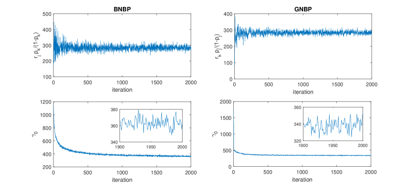
Figure 5: Trace plots of 2000 MCMC samples for example parameters of the BNBP (left column) and GNBP (right column) methods, applied to the BGI dataset.

We infer the model parameters via Gibbs sampling for the proposed BNP differential expression analysis algorithms. For each algorithm, we collect 1,000 MCMC samples after 1,000 burn-in iterations. The example MCMC sample trace plots in Figure 5 of the Appendix suggest that the Markov chains for both the GNBP and BNBP methods converge fast and mix well, supporting the practice of performing downstream analysis with 2,000 MCMC iterations. For the analysis of the real-world dataset BGI on a single cluster node with Intel Xeon 2.5GHz E5-2670 v2 processor, it took around two hours for both the GNBP and BNBP methods with 2,000 MCMC iterations, about ten minutes for the other methods, including the NBP. Note that parallelization could further speed up the inference. We use the collected MCMC samples to calculate the symmetric KL divergence, as in (23), between two groups for each gene, and rank the genes according to these values. For edgeR and DESeq, we follow the standard analysis pipelines and rank the genes using the computed $p$-values; and for baySeq, we rank the genes using model likelihoods. We set the fold change $b$ as $1.4$, $1.6$, $1.8$, or $2$ in simulating synthetic data to assess how sensitive the algorithms under study are to different levels of differential expression. For each fold change, we report the results of each algorithm based on ten independent random trials.

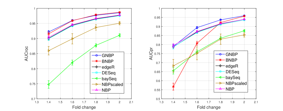
(a) GNBP synthetic data

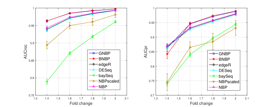
(b) BNBP synthetic data

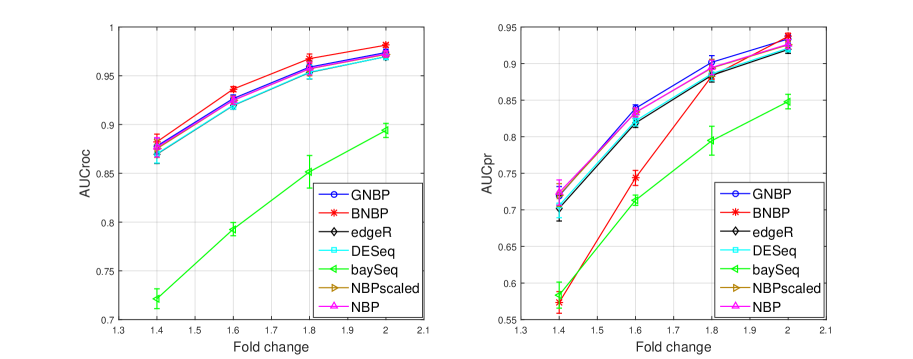
(c) baySeq synthetic data

Figure 1: left column: AUC-ROC values, right column: AUC-PR values. Performance comparison of different methods in detecting differentially expressed genes under various fold changes, using synthetic data generated under three different negative binomial distribution based models.

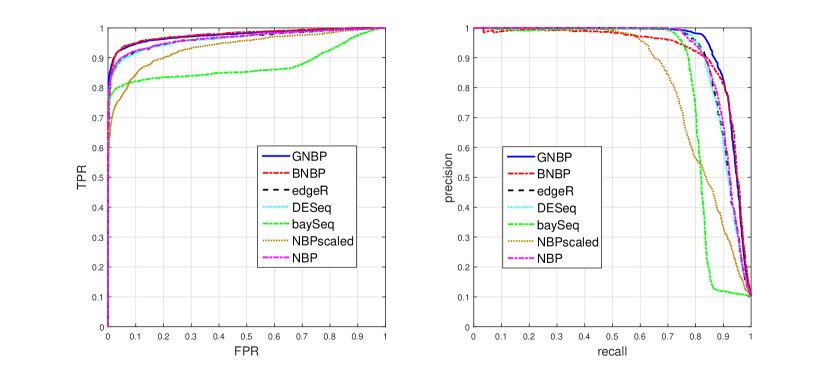
(a) GNBP setup

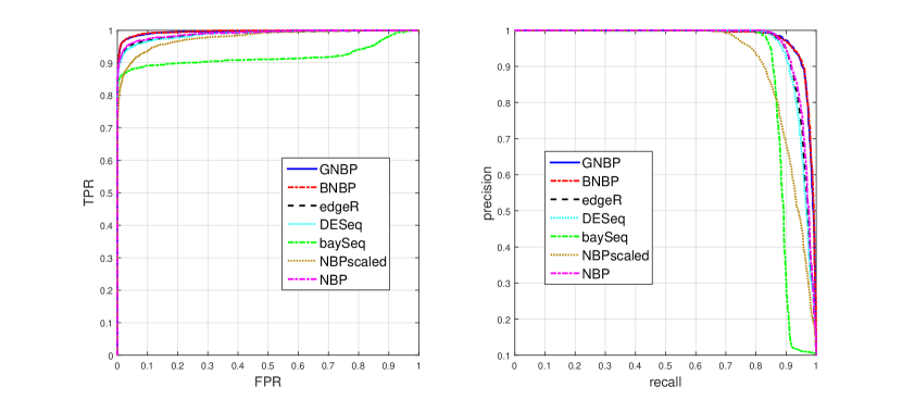
(b) BNBP setup

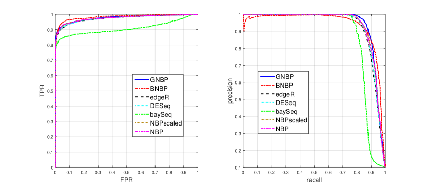
(c) baySeq setup

Figure 4: left column: ROC curve, right column: PR curve. Performance of different methods in detecting the differential expression of simulated data generated from different setups with a fold change of 1.8 for truly differentially expressed genes.

For these three different types of synthetic data, as shown in Figure 1, measured by both AUC-ROC and AUC-PR, baySeq has the worst overall performance even when the synthetic data are generated based on its model assumption, followed by the scaled NBP; the NBP, DESeq, and edgeR all have similar performance; and the GNBP and BNBP clearly outperform all the other differential expression analysis algorithms. To further compare the operating characteristics of different algorithms, we show in Figure 4 in the Appendix the full ROC and PR curves for the fold change of $b=1.8$. We provide in the Appendix the detailed numerical values used to plot Figure 1, as shown in Tables 1-6, where for each setting the best result and the ones that are less than one standard deviation away from the best are highlighted in bold.

More carefully examining Figures 1 and 4, it is interesting to notice that for the synthetic data generated with either the GNBP or BNBP, the scaled NBP, which extends the original NBP with sample-specific scaling parameters $q_{j}$ to model sample sequencing depth variations, in fact clearly underperforms the original NBP. Suggesting that explicitly modeling the sample sequencing depths, using the gamma-Poisson construction of the scaled NBP, is insufficient to model the over-dispersed gene counts generated using the gamma- or beta-NB constructions.

While the original NBP fixes $q_{j}=1$ and hence does not explicitly model the sample sequencing depth variations, it performs as well as both DESeq and edgeR in all three settings, which may be explained by the fact that it normalizes the posterior Poisson rates before applying them to compare the gene expression levels between two groups, a post-processing step that plays a similar role as the pre-processing normalization steps used in both DESeq and edgeR to account for different sequencing depths.

It is also interesting to notice that while the GNBP consistently ranks the best or very close to the best, in terms of both AUC-ROC and AUC-PR, the BNBP does so only in terms of AUC-ROC. For synthetic data generated using the GNBP and baySeq, the performance of the BNBP in terms of AUC-PR quickly deteriorates as the fold change reduces from 1.8 to 1.4, suggesting a large number of false positives among the top ranked genes of the BNBP when the fold change is not sufficiently large for the GNBP synthetic data. The disparity between the performance measured by AUC-ROC and that measured by AUC-PR, which only happens for the BNBP, indicates that the BNBP employs a distinct mechanism to detect differentially expressed genes, as carefully discussed below.

To compare the expression levels of the $k$th gene between two groups, the GNBP compares the posterior NB shape parameters $r_{k}$, whereas the BNBP compares the posterior NB probability parameters $p_{k}$. One may consider that the expression level of gene $k$ is assumed to roughly follow a smooth function of the shape parameter $r_{k}$ in the GNBP, and a smooth function of $p_{k}/(1-p_{k})$ in the BNBP. The difference between the posterior NB shape parameters $r_{k}$ explains the differences between both the means and dispersions, but does not explain that of the variance-to-mean ratios (VMR), of the counts of gene $k$ at different groups, since if $n_{jk}\sim\mbox{NB}(r_{k},p_{j})$, then $\mathbb{E}[n_{jk}]=r_{k}p_{j}/(1-p_{j}),~{}\mbox{var}[n_{jk}]=\mathbb{E}[n_{jk}]+(\mathbb{E}[n_{jk}])^{2}/r_{k}$, and $\mbox{VMR}[n_{jk}]=1+\mathbb{E}[n_{jk}]/r_{k}$; whereas the difference between the posterior NB probability parameters $p_{k}$ explains the differences between both the means and VMRs of the counts of gene $k$ at different groups, since if $n_{jk}\sim\mbox{NB}(r_{j},p_{k})$, then $\mathbb{E}[n_{jk}]=r_{j}p_{k}/(1-p_{k}),~{}\mbox{var}[n_{jk}]=\mathbb{E}[n_{jk}]+(\mathbb{E}[n_{jk}])^{2}/r_{j}$, and $\mbox{VMR}[n_{jk}]=1/(1-p_{k})$. Therefore, for the counts of a gene generated with the GNBP, if the $r_{k}$ is small, a small change in its value may lead to a significant change of $\mbox{VMR}[n_{jk}]=1+(\mathbb{E}[n_{jk}])/r_{k}$, which implies that a large difference in a gene’s VMRs between two groups may not be taken by the GNBP as a strong evidence for differential expression. By contrast, since the gene-specific parameter $p_{k}$ in the BNBP is explicitly responsible for the VMR, a large difference in a gene’s VMRs between two groups may encourage the BNBP to rank that gene as strongly differentially expressed, which may be used to explain why the BNBP has good AUC-ROC but poor AUC-PR if the fold change is small for the GNBP synthetic data. In practice, however, it is often unclear whether it is the change of the quadratic relationship between the variance and mean, as captured by the NB dispersion parameter, or the VMR, as captured by the NB probability parameter, that is responsible for the change of a gene’s expression level. Thus it is often unclear whether the GNBP or BNBP would be a better choice for a real dataset, and it seems promising to combine the advantages of both for differential expression analysis, an attractive research topic beyond the scope of the paper that is to be investigated in our future study.

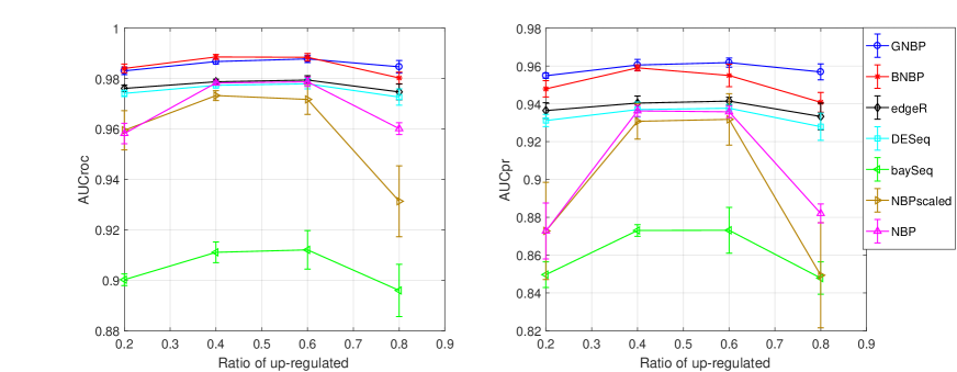
(a) Varying up/down-regulation proportions

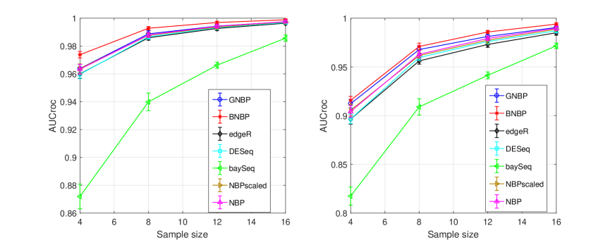
(b) Different sample sizes

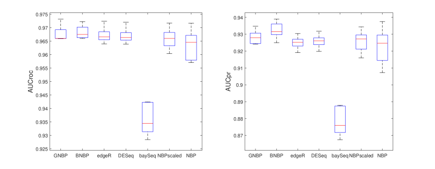
(c) Continuous true fold changes

Figure 6: left column: AUC-ROC values, right column: AUC-PR values. Performance comparison of different methods in detecting differentially expressed genes under various scenarios using synthetic data generated with baySeq. (a) The proportion of up-regulated genes in true differentially expressed genes increases from 20% to 80% with 20% increments. (b) The sample size in each group is increased from 4 to 16 with increments of size 4. (c) The true fold change of differentially expressed genes is sampled from a uniform distribution in the interval $[1.4,2]$.

To more comprehensively evaluate the proposed methods, we consider several additional application scenarios. The performance comparisons with baySeq synthetic data under these different scenarios are shown in Figure 6 in the Appendix. We first assess the sensitivity of different methods to the ratio of up- and down-regulated genes among the set of truly differentially expressed genes, which, the same as before, take 10% of the total number of genes. We assume a fold change of 2 for these truly differently expressed genes, and vary the percentage of up-regulated (down-regulated) genes among them from 20% (80%) to 40% (60%), 60% (40%), and 80% (20%). As shown in Figure 6(a), while the GNBP, BNBP, edgeR, and DESeq all show robustness to the change of that percentage, the performance of both the NBP based and baySeq methods significantly deteriorates as one increases the imbalance between the numbers of up- and down-regulated genes. We also note that both the GNBP and BNBP successfully preserve their out-performance margins under various ratios of up- to down-regulated genes.

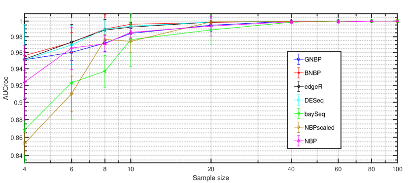
(a) AUC-ROC

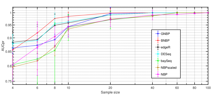
(b) AUC-PR

Figure 7: (a) AUC-ROC and (b) AUC-PR in the baySeq simulation setup with 100 genes and different sample sizes, where 10 genes are equally likely to be up- or down-regulated with a fold change of 2.

To examine how the performance changes with the sample size, we consider increasing the number of samples for each group from 4, to 8, 12, and 16. This is a sensible choice, since in practice the number of samples per condition is often smaller than 16. In this experiment, 10% of genes are equally likely to be up- or down-regulated with a fold change of 2. Figure 6(b) illustrates the error bar plots for both the AUC of ROC curve and that of PR curve, under different sample sizes over 10 random trials. All methods show consistent improvements as the number of replicates in each group increases, which agrees with the expectation that more samples provide more information to assist parameter inference. In addition, we consider 100 genes with different sample sizes to investigate the performance of the proposed methods in the setting with a large sample size but a small number of genes. Similar to previous simulations, 10% of the genes are assumed to be differentially expressed with a fold change of 2, and the number of replicates in each group is increased from 4 to 6, 8, 10, 20, 40, 60, 80, and 100. Figure 7 shows the error bar plots for both the AUC of ROC curve and that of PR curve, under different sample sizes over 10 random trials. As expected, adding more samples consistently enhances the recovery of true differential expression state of the genes for all methods, and when the number of samples reaches 100, almost all methods perform perfectly.

Last but not least, Figure 6(c) shows the box plots of the AUCs of ROC and PR curves when the true fold change of differentially expressed genes is uniformly distributed within the interval $[1.4,2]$. The BNBP stands out as the best performing method followed by the GNBP, suggesting that the superior results of the proposed methods in previous simulations do not rely on setting the fold change to a fixed constant.

4.2 SEQC benchmark RNA-Seq data and case study

In order to characterize various RNA-Seq technologies and quantification pipelines in the SEQC project (Xu et al., 2013; SEQC/MAQC-III Consortium, 2014), the same RNA samples for a comprehensive group of control genes are analyzed based on quantitative Reverse Transcription Polymerase Chain Reaction (qRT-PCR) using TaqMan assays (Joyce, 2002), which is referred as the TaqMan benchmark data (Shi et al., 2006; MAQC Consortium, 2010). For sample groups A and B, the expression intensity values of 955 selected control genes have been derived in the TaqMan qPT-PCR analysis for sequencing benchmarking. Without knowing in practice which genes are truly differentially expressed between different conditions, we consider thresholding the qRT-PCR expression ratios between different conditions at a certain value to define the ground-truth set of differentially expressed genes. Based on these 955 genes in the TaqMan data, we evaluate the performance of different differential expression analysis pipelines. Note that although the replicates in SEQC are technical, they show notable amount of over-dispersion and have been used in the literature as a standard benchmark for assessing differential expression analysis tools (Rapaport et al., 2013).

While it is unknown which genes are truly differentially expressed for both the BGI and PSU RNA-Seq data, we rely on the qRT-PCR expression intensity of the 955 genes in the TaqMan data and set different cut-offs for the binary logarithm (log2) of the qRT-PCR expression ratio to define “truly” differentially expressed genes. We increase this log2 cut-off value gradually from 0.5 to 2, and calculate both AUC-ROC and AUC-PR. The symmetric KL divergence is used to assess differential expression. As shown in Figure 2 for both the BGI and PSU datasets, the GNBP and BNBP outperform all the other methods in both ROC and PR analyses with significant margins. Note that the performance gains of the GNBP and BNBP over the other methods become more significant as one increases the log2 cut-off for the qRT-PCR expression ratio, which reduces the number of genes that are considered as truly differentially expressed.

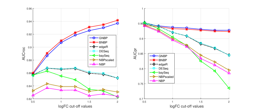
(a) BGI dataset

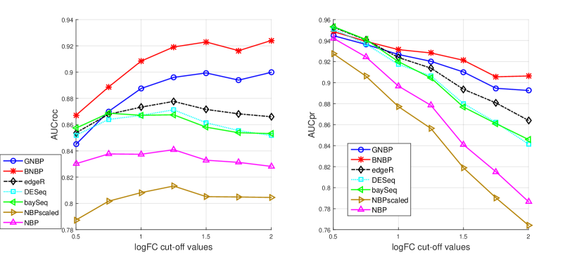
(b) PSU dataset

Figure 2: left column: AUC-ROC values, right column: AUC-PR values. Performance comparison of different methods in detecting differentially expressed genes on real-world benchmark RNA-Seq data from the SEQC project.

Comparing Figure 1 for synthetic data with Figure 2 for real-world data, one may notice that while both the AUC-ROC and AUC-PR curves in Figure 1 seem to monotonically increase as the fold change increases, the AUC-ROC and AUC-PR curves in Figure 2 do not necessarily share similar trends. It is not surprising to observe these seemingly distinct behaviors, since for the synthetic data in Figure 1, the set of truly differentially expressed genes are fixed and known exactly, remaining unchanged regardless of how one sets the fold change that is used to detect differentially expressed genes, whereas for the real-world data in Figure 2, the number of genes considered as truly expressed reduces as the cut-off value of the qRT-PCR expression ratio increases. In addition, we note that the results of edgeR, DESeq, and baySeq on both the BGI and PSU real datasets reported in this paper are similar to those reported in Rapaport et al. (2013).

To investigate the experimental results more thoroughly, we fix the true positives and negatives at the log2 cut-off value of 2 and illustrate the ROC and PR curves for BGI dataset in Figure 3. In addition, we show in Table 7 the area under the ROC curve for the range with $FPR\leq 0.1$ and area under the PR curve for the range with $\mbox{Recall}\leq 0.1$ for various algorithms. It is clear that both the GNBP and BNBP not only have higher AUC-ROC and AUC-PR, but also outperform all the other methods in almost all regions of the ROC and PR curves.

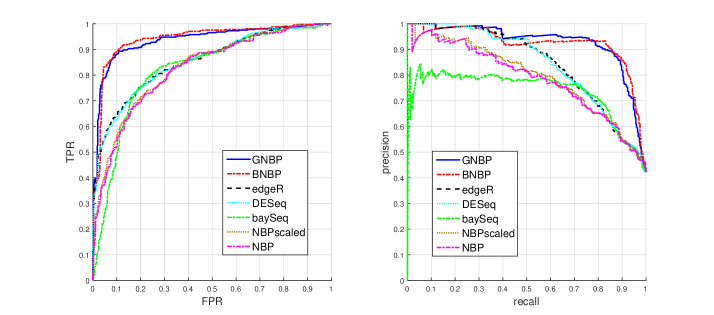
Figure 3: left: ROC curves, right: Precision-Recall (PR) curves. Performance comparison of different methods with the log2 cut-off value fixed at 2 for the BGI dataset from the SEQC project.

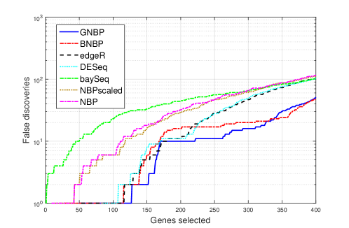
Figure 8: False discovery plots for different methods on the BGI dataset from the SEQC project, with the log2 cut-off value fixed at 2. The x-axis shows the number of genes selected, in order of their detected differential expression levels, while the y-axis shows the number of selected genes that are false positives.

In addition to showing the ROC and PR curves, we also plot the number of false discoveries to highlight the performance on the top ranked genes. Since there are 400 truly differentially expressed genes based on the log2 cut-off value of 2, the top 400 genes detected by each approach are selected and the number of false discoveries are plotted. It is clear from Figure 8 in the Appendix that both the GNBP and BNBP return much smaller number of false positives in comparison to all the other differential expression analysis algorithms.

4.3 Case study: clear cell renal cell carcinoma

For further illustration, we provide a case study with both the GNBP and BNBP methods on clear cell renal cell carcinoma (ccRCC), the most common type of kidney cancer that is closely related to genes involved in regulating cellular metabolism (Cancer Genome Atlas Research Network et al., 2012). We collect 21 samples from The Cancer Genome Atlas (TCGA) (McLendon et al., 2008), 11 of which are from the patients diagnosed with ccRCC and kidney as the primary site before any treatment procedures and the remaining 10 samples are from normal persons. These samples contain roughly 1.2 billion reads mapped to one of the 60,843 genomic locations annotated by the Ensembl database. The raw counts produced by HTSeq (Anders et al., 2014) are downloaded from the TCGA Website (see https://gdc-portal.nci.nih.gov/). We first filter out the genes whose total counts over all samples are less than 20. We apply both the GNBP and BNBP methods to detect differentially expressed genes, where after 1,000 burn-in iterations, 1,000 posterior samples are collected to calculate the KL-divergence between two different conditions to rank the genes. Similar to EdgeR and DESeq, our BNP based methods provide new statistical tools for differential expression analysis of RNA-Seq data and can help identify critical biomarkers in biomedical applications.

The top differentially expressed gene identified by the BNBP method is Interleukin-32 (IL-32), a proinflammatory cytokine that acts as a significant pathogenetic factor in various diseases and malignancies. It is reported as a potential prognostic factor for predicting outcomes in patients with ccRCC (Lee et al., 2012). The third gene in the ranking list is FHL1, for which clinical analyses suggest its expression is suppressed in some human tumors, including those of the breast, kidney, and prostate and it suppresses metastatic cell growth (Li et al., 2008). The fourth gene, VIM, is another potential oncogene regulated by tumor suppressive microRNA-138 (Yamasaki et al., 2012). The fifth gene, Progranulin (PGRN), is a pluripotent secreted growth factor that mediates cell cycle progression and cell motility, and is highly expressed in aggressive cancer cell lines and clinical specimens, including breast, ovarian, and renal cancers as well as gliomas (He and Bateman, 2003). The ninth gene, SLC12A1, is a tumor suppressor that is reported to lose its function in ccRCC as a result of increased levels of some microRNAs such as miR-142-3p and miR-185 (Liu et al., 2010). The tenth gene, PGK1, is a target gene of MYC pathway, which potentially has an essential role in the proliferation of ccRCC cells (Tang et al., 2009).

The top differentially expressed gene identified by the GNBP method is UMOD, encoding uromodulin, the major protein secreted in the normal urine that has a link to kidney chronic disease. It has been considered as a potential therapeutic target to preserve renal function (Trudu et al., 2013). The fourth gene, MT-ND4, is a mitochondrial gene whose mutation leads to complex I enzyme deficiency found in renal oncocytoma (Gasparre et al., 2008). The seventh gene, AQP2, involved in regulating the homeostasis of water-electrolyte balances has been found to be the most significantly down-regulated in ccRCCs (Zhou et al., 2010). The ninth gene, COX-2 is associated with several clinicopathological factors, and is conjectured to play an important role in tumor cell proliferation and MMP-2 expression (Miyata et al., 2003).

In addition to these top ranked genes, several other important genes, previously shown to have strong connections to renal cell carcinoma, are also ranked in the top 5% by both the GNBP and BNBP methods. In the following we list some well-studied ccRCC biomarkers or genetic risk factors in the literature.

• The CA9 gene, whose corresponding encoded protein is a tumor-associated antigen, is well known in the literature as a reliable diagnostic biomarker of clear cell carcinoma of kidney (Liao et al., 1997; Bui et al., 2003).

• The MT1G gene has been demonstrated to have frequent occurrence of Methylation of CpG dinucleotides in the promoter region, which is a major mechanism of tumor suppressor genes inactivation in renal cell carcinoma (Morris et al., 2003).

• A member of the AP-2 family of transcription factors, TFAP2B, functions as both a transcriptional activator and repressor, required for proper terminal differentiation and function of renal tubular epithelia for the survival of renal epithelial cells during renal development (Tun et al., 2010). Its down-regulation in ccRCC has been verified by Microarray profiling and PCR (Tun et al., 2010).

• The DACH1 gene is a molecular marker of renal cell carcinoma where its expression remarkably decreases and the restoration of DACH1 function in renal clear cell cancer cells inhibits in vitro cellular proliferation, S phase progression, clone formation, and in vivo tumor growth (Chu et al., 2014).

• ANGPT2 is a member of the angiopoietin family, which plays a pivotal role in angiogenesis during cancer development and metastasis (Lu et al., 2014). Upregulation of ANGPT2 has been reported in various human cancers including renal cell carcinoma (Bullock et al., 2010; Baldewijns et al., 2007).

5 Conclusions

We exploit Bayesian nonparametric priors, including the gamma-Poisson, gamma-negative binomial, and beta-negative binomial processes, to model RNA sequencing count matrices. With different sequencing depths captured by sample-specific model parameters, the posterior distributions of certain gene-specific model parameters are used to detect the genes that are differentially expressed between different conditions. With the model parameters inferred by borrowing statistical strength across both the genes and samples, there is no need to adjust the raw counts using heuristics before downstream analyses, an important pre-processing step that is often required in previously proposed algorithms. Example results on both synthetic and real-world RNA-Seq data demonstrate the state-of-the-art performance of both the gamma- and beta-negative binomial processes based differential expression analysis algorithms. Given the success of the proposed random-process-based algorithms in differential expression analysis, it is of interest to investigate Bayesian nonparametric algorithms for many other real-world applications in biomedicine that require analyzing next-generation sequencing data.

6 Acknowledgments

We thank the editor and three reviewers for insightful and constructive comments and suggestions. We thank Texas A&M High Performance Research Computing and Texas Advanced Computing Center for providing computational resources to perform experiments in this paper. X. Qian acknowledges the support of CAREER award 1553281 from the U.S. National Science Foundation.

Supplementary Material for BNP-Seq: Bayesian Nonparametric Differential Expression Analysis of Sequencing Count Data

Appendix A Chinese restaurant table (CRT) distribution

The negative binomial distribution $m\sim\mbox{NB}(r,p)$ with the probability mass function

$$f_{M}(m)=\frac{\Gamma(m+r)}{m!\Gamma(r)}(1-p)^{r}p^{m},~{}~{}m\in\{0,1,\ldots\}$$

can be augmented as a gamma mixed Poisson distribution as

$$m\sim\mbox{Pois}(\lambda),~{}\lambda\sim\mbox{Gamma}(r,p/(1-p)),$$

where the gamma distribution is parametrized by its shape $r$ and scale $p/(1-p)$. It can be augmented under a compound Poisson representation as

$$m=\sum_{t=1}^{\ell}u_{t},~{}u_{t}\sim\mbox{Log}(p),~{}\ell\sim\mbox{Pois}(-r\ln(1-p)),$$

where $u\sim\mbox{Log}(p)$ is the logarithmic distribution with probability generation function $C_{U}(z)=\ln(1-pz)/\ln(1-p)$, $|z|<p^{-1}$. As in Zhou and Carin (2015), we denote the conditional posterior distribution of $\ell$ given $m$ and $r$ by $(\ell\,|\,m,r)\sim\mbox{CRT}(m,r)$ and sample it with the summation of independent Bernoulli random variables as $\ell=\sum_{n=1}^{m}b_{n}$, $b_{n}\sim\mbox{Bernoulli}[r/(n-1+r)]$.

Appendix B Additional tables and figures

Table 1: AUC-ROC in the GNBP simulation setup for different true fold changes.

	Fold change
Method	1.4	1.6	1.8	2
GNBP	0.9226 $\pm$ 0.006	0.9625 $\pm$ 0.003	0.9777 $\pm$ 0.003	0.9864 $\pm$ 0.002
BNBP	0.9156 $\pm$ 0.005	0.9610 $\pm$ 0.003	0.9783 $\pm$ 0.002	0.9875 $\pm$ 0.002
edgeR	0.9004 $\pm$ 0.007	0.9463 $\pm$ 0.004	0.9653 $\pm$ 0.003	0.9778 $\pm$ 0.003
DESeq	0.8986 $\pm$ 0.008	0.9444 $\pm$ 0.004	0.9634 $\pm$ 0.003	0.9764 $\pm$ 0.003
baySeq	0.7542 $\pm$ 0.008	0.8247 $\pm$ 0.012	0.8752 $\pm$ 0.003	0.9114 $\pm$ 0.008
NBP	0.9035 $\pm$ 0.007	0.9476 $\pm$ 0.004	0.9665 $\pm$ 0.003	0.9786 $\pm$ 0.003
NBPscaled	0.8596 $\pm$ 0.014	0.8990 $\pm$ 0.017	0.9366 $\pm$ 0.009	0.9506 $\pm$ 0.0053

Table 2: AUC-PR in the GNBP simulation setup for different true fold changes.

	Fold change
Method	1.4	1.6	1.8	2
GNBP	0.7873 $\pm$ 0.011	0.8998 $\pm$ 0.006	0.9382 $\pm$ 0.003	0.9607 $\pm$ 0.003
BNBP	0.5660 $\pm$ 0.011	0.8189 $\pm$ 0.008	0.9213 $\pm$ 0.005	0.9563 $\pm$ 0.002
edgeR	0.7857 $\pm$ 0.015	0.8742 $\pm$ 0.007	0.9136 $\pm$ 0.003	0.9403 $\pm$ 0.003
DESeq	0.7848 $\pm$ 0.014	0.8714 $\pm$ 0.007	0.9107 $\pm$ 0.002	0.9369 $\pm$ 0.004
baySeq	0.6517 $\pm$ 0.012	0.7655 $\pm$ 0.015	0.8329 $\pm$ 0.003	0.8756 $\pm$ 0.004
NBP	0.7934 $\pm$ 0.014	0.8770 $\pm$ 0.007	0.9156 $\pm$ 0.003	0.9399 $\pm$ 0.003
NBPscaled	0.6822 $\pm$ 0.035	0.7515 $\pm$ 0.036	0.8298 $\pm$ 0.028	0.8533 $\pm$ 0.012

Table 3: AUC-ROC in the BNBP simulation setup for different true fold changes.

	Fold change
Method	1.4	1.6	1.8	2
GNBP	0.9648 $\pm$ 0.001	0.9847 $\pm$ 0.001	0.9914 $\pm$ 0.0014	0.9968 $\pm$ 0.001
BNBP	0.9635 $\pm$ 0.001	0.9848 $\pm$ 0.002	0.9922 $\pm$ 0.0009	0.9971 $\pm$ 0.0009
edgeR	0.9399 $\pm$ 0.001	0.9706 $\pm$ 0.003	0.9829 $\pm$ 0.0017	0.9929 $\pm$ 0.00189
DESeq	0.9383 $\pm$ 0.002	0.9694 $\pm$ 0.003	0.9818 $\pm$ 0.0016	0.9920 $\pm$ 0.0018
baySeq	0.7919 $\pm$ 0.007	0.8699 $\pm$ 0.07	0.9167 $\pm$ 0.007	0.9590 $\pm$ 0.0041
NBP	0.9438 $\pm$ 0.001	0.9729 $\pm$ 0.003	0.9844 $\pm$ 0.002	0.9935 $\pm$ 0.0016
NBPscaled	0.8939 $\pm$ 0.0107	0.9499 $\pm$ 0.0092	0.9606 $\pm$ 0.0094	0.9811 $\pm$ 0.008

Table 4: AUC-PR in the BNBP simulation setup for different true fold changes.

	Fold change
Method	1.4	1.6	1.8	2
GNBP	0.8632 $\pm$ 0.011	0.9431 $\pm$ 0.005	0.9703 $\pm$ 0.003	0.9881 $\pm$ 0.002
BNBP	0.8356 $\pm$ 0.012	0.9432 $\pm$ 0.003	0.9725 $\pm$ 0.002	0.9889 $\pm$ 0.003
edgeR	0.8674 $\pm$ 0.006	0.9275 $\pm$ 0.005	0.9557 $\pm$ 0.003	0.9783 $\pm$ 0.004
DESeq	0.8634 $\pm$ 0.004	0.9240 $\pm$ 0.005	0.9523 $\pm$ 0.003	0.9759 $\pm$ 0.003
baySeq	0.7413 $\pm$ 0.015	0.8408 $\pm$ 0.01	0.8963 $\pm$ 0.007	0.9434 $\pm$ 0.003
NBP	0.8708 $\pm$ 0.006	0.9302 $\pm$ 0.005	0.9577 $\pm$ 0.003	0.9798 $\pm$ 0.003
NBPscaled	0.7450 $\pm$ 0.03	0.8648 $\pm$ 0.019	0.8846 $\pm$ 0.028	0.9318 $\pm$ 0.025

Table 5: AUC-ROC in the baySeq simulation setup for different true fold changes.

	Fold change
Method	1.4	1.6	1.8	2
GNBP	0.8772 $\pm$ 0.009	0.9286 $\pm$ 0.005	0.9585 $\pm$ 0.004	0.9738 $\pm$ 0.001
BNBP	0.8823 $\pm$ 0.005	0.9382 $\pm$ 0.004	0.9674 $\pm$ 0.003	0.9812 $\pm$ 0.0015
edgeR	0.8702 $\pm$ 0.008	0.9216 $\pm$ 0.0042	0.9518 $\pm$ 0.004	0.9687 $\pm$ 0.003
DESeq	0.8705 $\pm$ 0.0083	0.9220 $\pm$ 0.004	0.9520 $\pm$ 0.0036	0.9688 $\pm$ 0.003
baySeq	0.7222 $\pm$ 0.0089	0.7887 $\pm$ 0.0067	0.8489 $\pm$ 0.012	0.8911 $\pm$ 0.0099
NBP	0.8769 $\pm$ 0.0075	0.9270 $\pm$ 0.0045	0.9567 $\pm$ 0.0031	0.9725 $\pm$ 0.0026
NBPscaled	0.8752 $\pm$ 0.009	0.9248 $\pm$ 0.0044	0.9571 $\pm$ 0.0071	0.9719 $\pm$ 0.0031

Table 6: AUC-PR in the baySeq simulation setup for different true fold changes.

	Fold change
Method	1.4	1.6	1.8	2
GNBP	0.7194 $\pm$ 0.015	0.8372 0.0095 $\pm$	0.8984 $\pm$ 0.0074	0.9332 $\pm$ 0.0041
BNBP	0.5733 $\pm$ 0.012	0.7448 $\pm$ 0.014	0.8826 $\pm$ 0.0055	0.9337 $\pm$ 0.0058
edgeR	0.7004 $\pm$ 0.013	0.8152 $\pm$ 0.008	0.8787 $\pm$ 0.0066	0.9173 $\pm$ 0.0054
DESeq	0.7042 $\pm$ 0.013	0.8180 $\pm$ 0.0082	0.8813 $\pm$ 0.0058	0.9194 $\pm$ 0.005
baySeq	0.5806 $\pm$ 0.0096	0.7034 $\pm$ 0.0057	0.7877 $\pm$ 0.0104	0.8482 $\pm$ 0.0106
NBP	0.7223 $\pm$ 0.0129	0.8312 $\pm$ 0.0075	0.8913 $\pm$ 0.0058	0.9248 $\pm$ 0.0055
NBPscaled	0.7203 $\pm$ 0.0155	0.8333 $\pm$ 0.006	0.8940 $\pm$ 0.012	0.9256 $\pm$ 0.0047

Table 7: Area under the ROC curve for the range with $FPR\leq 0.1$ and area under the PR curve for the range with $\mbox{Recall}\leq 0.1$ for both the PSU and BGI datasets, with the log2 cut-off value fixed at 2.

	PSU		BGI
Method	AUCroc	AUCpr	AUCroc	AUCpr
GNBP	0.0627	0.0980	0.0716	0.0995
BNBP	0.0628	0.0980	0.0685	0.0986
edgeR	0.0587	0.0980	0.0527	0.0995
DESeq	0.0514	0.0980	0.0521	0.0995
baySeq	0.0533	0.0980	0.0258	0.0757
NBP	0.0356	0.0921	0.0390	0.0968
NBPscaled	0.0404	0.0911	0.0369	0.0957

References

- Anders and Huber [2010] S. Anders and W. Huber. Differential expression analysis for sequence count data. Genome Biology, 11(10):R106, 2010.
- Anders et al. [2014] S. Anders, P. T. Pyl, and W. Huber. Htseq–a python framework to work with high-throughput sequencing data. Bioinformatics, page btu638, 2014.
- Baldewijns et al. [2007] M. Baldewijns, V. Thijssen, G. Van den Eynden, S. Van Laere, A. Bluekens, T. Roskams, H. Van Poppel, A. De Bruine, A. Griffioen, and P. Vermeulen. High-grade clear cell renal cell carcinoma has a higher angiogenic activity than low-grade renal cell carcinoma based on histomorphological quantification and qrt–pcr mrna expression profile. British Journal of Cancer, 96(12):1888–1895, 2007.
- Bliss and Fisher [1953] C. I. Bliss and R. A. Fisher. Fitting the negative binomial distribution to biological data. Biometrics, 9(2):176–200, 1953.
- Broderick et al. [2015] T. Broderick, L. Mackey, J. Paisley, and M. I. Jordan. Combinatorial clustering and the beta negative binomial process. IEEE Trans. Pattern Anal. Mach. Intell., 2015.
- Bui et al. [2003] M. H. Bui, D. Seligson, K.-r. Han, A. J. Pantuck, F. J. Dorey, Y. Huang, S. Horvath, B. C. Leibovich, S. Chopra, S.-Y. Liao, et al. Carbonic anhydrase ix is an independent predictor of survival in advanced renal clear cell carcinoma implications for prognosis and therapy. Clinical Cancer Research, 9(2):802–811, 2003.
- Bullard et al. [2010] J. H. Bullard, E. Purdom, K. D. Hansen, and S. Dudoit. Evaluation of statistical methods for normalization and differential expression in mRNA-Seq experiments. BMC Bioinformatics, 11(1):94, 2010.
- Bullock et al. [2010] A. Bullock, L. Zhang, A. O’Neill, A. Percy, V. Sukhatme, J. Mier, M. Atkins, and R. Bhatt. Plasma angiopoietin-2 (ang2) as an angiogenic biomarker in renal cell carcinoma (rcc). In ASCO Annual Meeting Proceedings, volume 28, page 4630, 2010.
- Cancer Genome Atlas Research Network et al. [2012] Cancer Genome Atlas Research Network et al. Comprehensive molecular characterization of clear cell renal cell carcinoma. Nature, 499(7456):43–49, 2012.
- Caron et al. [2014] F. Caron, Y. W. Teh, and B. T. Murphy. Bayesian nonparametric Plackett-Luce models for the analysis of clustered ranked data. Annal of Applied Statistics, 2014.
- Chu et al. [2014] Q. Chu, N. Han, X. Yuan, X. Nie, H. Wu, Y. Chen, M. Guo, S. Yu, and K. Wu. Dach1 inhibits cyclin d1 expression, cellular proliferation and tumor growth of renal cancer cells. Journal of Hematology & Oncology, 7(1):1, 2014.
- Datta and Nettleton [2014] S. Datta and D. Nettleton. Statistical Analysis of Next Generation Sequencing Data. Frontiers in Probability and the Statistical Sciences. Springer International Publishing, 2014.
- Dillies et al. [2013] M.-A. Dillies, A. Rau, J. Aubert, C. Hennequet-Antier, M. Jeanmougin, N. Servant, C. Keime, G. Marot, D. Castel, J. Estelle, et al. A comprehensive evaluation of normalization methods for illumina high-throughput RNA sequencing data analysis. Briefings in Bioinformatics, 14(6):671–683, 2013.
- Ferguson [1973] T. S. Ferguson. A Bayesian analysis of some nonparametric problems. Ann. Statist., 1(2):209–230, 1973.
- Gasparre et al. [2008] G. Gasparre, E. Hervouet, E. de Laplanche, J. Demont, L. F. Pennisi, M. Colombel, F. Mège-Lechevallier, J.-Y. Scoazec, E. Bonora, R. Smeets, et al. Clonal expansion of mutated mitochondrial dna is associated with tumor formation and complex i deficiency in the benign renal oncocytoma. Human Molecular Genetics, 17(7):986–995, 2008.
- Gentleman et al. [2004] R. C. Gentleman, V. J. Carey, D. M. Bates, B. Bolstad, M. Dettling, S. Dudoit, B. Ellis, L. Gautier, Y. Ge, J. Gentry, et al. Bioconductor: open software development for computational biology and bioinformatics. Genome Biology, 5(10):R80, 2004.
- Greenwood and Yule [1920] M. Greenwood and G. U. Yule. An inquiry into the nature of frequency distributions representative of multiple happenings with particular reference to the occurrence of multiple attacks of disease or of repeated accidents. J. R. Stat. Soc., 1920.
- Hardcastle and Kelly [2010] T. J. Hardcastle and K. A. Kelly. bayseq: empirical bayesian methods for identifying differential expression in sequence count data. BMC Bioinformatics, 11(1):422, 2010.
- He and Bateman [2003] Z. He and A. Bateman. Progranulin (granulin-epithelin precursor, pc-cell-derived growth factor, acrogranin) mediates tissue repair and tumorigenesis. Journal of Molecular Medicine, 81(10):600–612, 2003.
- Hjort [1990] N. L. Hjort. Nonparametric Bayes estimators based on beta processes in models for life history data. Ann. Statist., 1990.
- Joyce [2002] C. Joyce. Quantitative rt-pcr. RT-PCR Protocols, pages 83–92, 2002.
- Kingman [1993] J. F. C. Kingman. Poisson Processes. Oxford University Press, 1993.
- Kullback and Leibler [1951] S. Kullback and R. A. Leibler. On information and sufficiency. Annals of Mathematical Statistics, 22(1):79–86, 1951.
- Lee et al. [2012] H.-J. Lee, Z. L. Liang, S. M. Huang, J.-S. Lim, D.-Y. Yoon, H.-J. Lee, and J. M. Kim. Overexpression of il-32 is a novel prognostic factor in patients with localized clear cell renal cell carcinoma. Oncology Letters, 3(2):490–496, 2012.
- Li and Tibshirani [2013] J. Li and R. Tibshirani. Finding consistent patterns: a nonparametric approach for identifying differential expression in RNA-Seq data. Statistical Methods in Medical Research, 22(5):519–536, 2013.
- Li et al. [2011] J. Li, D. M. Witten, I. M. Johnstone, and R. Tibshirani. Normalization, testing, and false discovery rate estimation for RNA-sequencing data. Biostatistics, page kxr031, 2011.
- Li et al. [2008] X. Li, Z. Jia, Y. Shen, H. Ichikawa, J. Jarvik, R. G. Nagele, and G. S. Goldberg. Coordinate suppression of sdpr and fhl1 expression in tumors of the breast, kidney, and prostate. Cancer Science, 99(7):1326–1333, 2008.
- Liao et al. [1997] S.-Y. Liao, O. N. Aurelio, K. Jan, J. Zavada, and E. J. Stanbridge. Identification of the mn/ca9 protein as a reliable diagnostic biomarker of clear cell carcinoma of the kidney. Cancer Research, 57(14):2827–2831, 1997.
- Liu et al. [2010] H. Liu, A. R. Brannon, A. R. Reddy, G. Alexe, M. W. Seiler, A. Arreola, J. H. Oza, M. Yao, D. Juan, L. S. Liou, et al. Identifying mrna targets of microrna dysregulated in cancer: with application to clear cell renal cell carcinoma. BMC Systems Biology, 4(1):1, 2010.
- Lorenz et al. [2014] D. J. Lorenz, R. S. Gill, R. Mitra, and S. Datta. Using RNA-seq data to detect differentially expressed genes. In Statistical Analysis of Next Generation Sequencing Data, pages 25–49. Springer, 2014.
- Love et al. [2014] M. I. Love, W. Huber, and S. Anders. Moderated estimation of fold change and dispersion for RNA-seq data with DESeq2. Genome Biology, 15(12):1–21, 2014.
- Lovén et al. [2012] J. Lovén, D. A. Orlando, A. A. Sigova, C. Y. Lin, P. B. Rahl, C. B. Burge, D. L. Levens, T. I. Lee, and R. A. Young. Revisiting global gene expression analysis. Cell, 151(3):476–482, 2012.
- Lu et al. [2014] R. Lu, Z. Ji, X. Li, Q. Zhai, C. Zhao, Z. Jiang, S. Zhang, L. Nie, and Z. Yu. mir-145 functions as tumor suppressor and targets two oncogenes, angpt2 and nedd9, in renal cell carcinoma. Journal of Cancer Research and Clinical Oncology, 140(3):387–397, 2014.
- MAQC Consortium [2010] MAQC Consortium. The MicroArray Quality Control (MAQC)-II study of common practices for the development and validation of microarray-based predictive models. Nature Biotechnology, 28(8):827–838, 2010.
- McLendon et al. [2008] R. McLendon, A. Friedman, D. Bigner, E. G. Van Meir, D. J. Brat, G. M. Mastrogianakis, J. J. Olson, T. Mikkelsen, N. Lehman, K. Aldape, et al. Comprehensive genomic characterization defines human glioblastoma genes and core pathways. Nature, 455(7216):1061–1068, 2008.
- Metzker [2010] M. L. Metzker. Sequencing technologies—the next generation. Nature Reviews Genetics, 11(1):31–46, 2010.
- Miyata et al. [2003] Y. Miyata, S. Koga, S. Kanda, M. Nishikido, T. Hayashi, and H. Kanetake. Expression of cyclooxygenase-2 in renal cell carcinoma correlation with tumor cell proliferation, apoptosis, angiogenesis, expression of matrix metalloproteinase-2, and survival. Clinical Cancer Research, 9(5):1741–1749, 2003.
- Morris et al. [2003] M. R. Morris, L. B. Hesson, K. J. Wagner, N. V. Morgan, D. Astuti, R. D. Lees, W. N. Cooper, J. Lee, D. Gentle, F. Macdonald, et al. Multigene methylation analysis of wilms’ tumour and adult renal cell carcinoma. Oncogene, 22(43):6794–6801, 2003.
- Mortazavi et al. [2008] A. Mortazavi, B. A. Williams, K. McCue, L. Schaeffer, and B. Wold. Mapping and quantifying mammalian transcriptomes by RNA-Seq. Nature methods, 5(7):621–628, 2008.
- Oshlack et al. [2010] A. Oshlack, M. D. Robinson, and M. D. Young. From RNA-seq reads to differential expression results. Genome Biology, 11(12):1–10, 2010.
- Rapaport et al. [2013] F. Rapaport, R. Khanin, Y. Liang, M. Pirun, A. Krek, P. Zumbo, C. E. Mason, N. D. Socci, and D. Betel. Comprehensive evaluation of differential gene expression analysis methods for RNA-seq data. Genome Biology, 14(9):R95, 2013.
- Risso et al. [2014a] D. Risso, J. Ngai, T. P. Speed, and S. Dudoit. Normalization of rna-seq data using factor analysis of control genes or samples. Nature Biotechnology, 32(9):896–902, 2014a.
- Risso et al. [2014b] D. Risso, J. Ngai, T. P. Speed, and S. Dudoit. The role of spike-in standards in the normalization of RNA-seq. In Statistical Analysis of Next Generation Sequencing Data, pages 169–190. Springer, 2014b.
- Roberts et al. [2011] A. Roberts, C. Trapnell, J. Donaghey, J. L. Rinn, and L. Pachter. Improving RNA-Seq expression estimates by correcting for fragment bias. Genome biology, 12(3):1, 2011.
- Robinson and Oshlack [2010] M. D. Robinson and A. Oshlack. A scaling normalization method for differential expression analysis of RNA-seq data. Genome Biology, 11(3):1–9, 2010.
- Robinson and Smyth [2007] M. D. Robinson and G. K. Smyth. Moderated statistical tests for assessing differences in tag abundance. Bioinformatics, 23(21):2881–2887, 2007.
- Robinson et al. [2010] M. D. Robinson, D. J. McCarthy, and G. K. Smyth. edger: a bioconductor package for differential expression analysis of digital gene expression data. Bioinformatics, 26(1):139–140, 2010.
- Schena et al. [1995] M. Schena, D. Shalon, R. W. Davis, and P. O. Brown. Quantitative monitoring of gene expression patterns with a complementary DNA microarray. Science, 270(5235):467, 1995.
- Schurch et al. [2016] N. J. Schurch, P. Schofield, M. Gierliński, C. Cole, A. Sherstnev, V. Singh, N. Wrobel, K. Gharbi, G. G. Simpson, T. Owen-Hughes, et al. How many biological replicates are needed in an RNA-seq experiment and which differential expression tool should you use? RNA, 22(6):839–851, 2016.
- SEQC/MAQC-III Consortium [2014] SEQC/MAQC-III Consortium. A comprehensive assessment of RNA-seq accuracy, reproducibility and information content by the Sequencing Quality Control Consortium. Nature Biotechnology, 32(9):903–914, 2014.
- Shi et al. [2006] L. Shi, L. H. Reid, W. D. Jones, R. Shippy, J. A. Warrington, S. C. Baker, P. J. Collins, F. De Longueville, E. S. Kawasaki, K. Y. Lee, et al. The microarray quality control (maqc) project shows inter-and intraplatform reproducibility of gene expression measurements. Nature Biotechnology, 24(9):1151–1161, 2006.
- Smyth and Verbyla [1996] G. Smyth and A. Verbyla. A conditional likelihood approach to residual maximum likelihood estimation in generalized linear models. J. R. Stat. Soc: Series B, 58(3):565–572, 1996.
- Soneson and Delorenzi [2013] C. Soneson and M. Delorenzi. A comparison of methods for differential expression analysis of RNA-seq data. BMC Bioinformatics, 14:91, 2013.
- Tang et al. [2009] S.-W. Tang, W.-H. Chang, Y.-C. Su, Y.-C. Chen, Y.-H. Lai, P.-T. Wu, C.-I. Hsu, W.-C. Lin, M.-K. Lai, and J.-Y. Lin. Myc pathway is activated in clear cell renal cell carcinoma and essential for proliferation of clear cell renal cell carcinoma cells. Cancer Letters, 273(1):35–43, 2009.
- Trudu et al. [2013] M. Trudu, S. Janas, C. Lanzani, H. Debaix, C. Schaeffer, M. Ikehata, L. Citterio, S. Demaretz, F. Trevisani, G. Ristagno, et al. Common noncoding umod gene variants induce salt-sensitive hypertension and kidney damage by increasing uromodulin expression. Nature Medicine, 19(12):1655–1660, 2013.
- Tun et al. [2010] H. W. Tun, L. A. Marlow, C. A. Von Roemeling, S. J. Cooper, P. Kreinest, K. Wu, B. A. Luxon, M. Sinha, P. Z. Anastasiadis, and J. A. Copland. Pathway signature and cellular differentiation in clear cell renal cell carcinoma. PloS One, 5(5):e10696, 2010.
- Wang et al. [2010] L. Wang, Z. Feng, X. Wang, X. Wang, and X. Zhang. DEGseq: an R package for identifying differentially expressed genes from RNA-seq data. Bioinformatics, 26(1):136–138, 2010.
- Wang et al. [2009] Z. Wang, M. Gerstein, and M. Snyder. RNA-Seq: a revolutionary tool for transcriptomics. Nature Reviews Genetics, 10(1):57–63, 2009.
- West [2003] M. West. Bayesian factor regression models in the “large , small ” paradigm. In Bayesian Statistics, 2003.
- Xu et al. [2013] J. Xu, Z. Su, H. Hong, J. Thierry-Mieg, D. Thierry-Mieg, D. P. Kreil, C. E. Mason, W. Tong, and L. Shi. Cross-platform ultradeep transcriptomic profiling of human reference RNA samples by RNA-Seq. Scientific Data, 1:140020–140020, 2013.
- Yamasaki et al. [2012] T. Yamasaki, N. Seki, Y. Yamada, H. Yoshino, H. Hidaka, T. Chiyomaru, N. Nohata, T. Kinoshita, M. Nakagawa, and H. Enokida. Tumor suppressive microrna-138 contributes to cell migration and invasion through its targeting of vimentin in renal cell carcinoma. International Journal of Oncology, 41(3):805–817, 2012.
- Zhang et al. [2014] Z. H. Zhang, D. J. Jhaveri, V. M. Marshall, D. C. Bauer, J. Edson, R. K. Narayanan, G. J. Robinson, A. E. Lundberg, P. F. Bartlett, N. R. Wray, et al. A comparative study of techniques for differential expression analysis on RNA-Seq data. PloS one, 9(8):e103207, 2014.
- Zhou et al. [2010] L. Zhou, J. Chen, Z. Li, X. Li, X. Hu, Y. Huang, X. Zhao, C. Liang, Y. Wang, L. Sun, et al. Integrated profiling of micrornas and mrnas: micrornas located on xq27. 3 associate with clear cell renal cell carcinoma. PloS One, 5(12):e15224, 2010.
- Zhou and Carin [2015] M. Zhou and L. Carin. Negative binomial process count and mixture modeling. IEEE Trans. Pattern Anal. Mach. Intell., 37(2):307–320, 2015.
- Zhou et al. [2012] M. Zhou, L. Hannah, D. Dunson, and L. Carin. Beta-negative binomial process and Poisson factor analysis. In AISTATS, pages 1462–1471, 2012.
- Zhou et al. [2016] M. Zhou, O. H. M. Padilla, and J. G. Scott. Priors for random count matrices derived from a family of negative binomial processes. J. Amer. Statist. Assoc., 111(515):1144–1156, 2016.
- Zyprych-Walczak et al. [2015] J. Zyprych-Walczak, A. Szabelska, L. Handschuh, K. Górczak, K. Klamecka, M. Figlerowicz, and I. Siatkowski. The impact of normalization methods on RNA-Seq data analysis. BioMed Research International, 2015, 2015.