Identifying parameter regions for multistationarity

Abstract

Mathematical modelling has become an established tool for studying the dynamics of biological systems. Current applications range from building models that reproduce quantitative data to identifying systems with predefined qualitative features, such as switching behaviour, bistability or oscillations. Mathematically, the latter question amounts to identifying parameter values associated with a given qualitative feature.

We introduce a procedure to partition the parameter space of a parameterized system of ordinary differential equations into regions for which the system has a unique or multiple equilibria. The procedure is based on the computation of the Brouwer degree, and it creates a multivariate polynomial with parameter depending coefficients. The signs of the coefficients determine parameter regions with and without multistationarity. A particular strength of the procedure is the avoidance of numerical analysis and parameter sampling.

The procedure consists of a number of steps. Each of these steps might be addressed algorithmically using various computer programs and available software, or manually. We demonstrate our procedure on several models of gene transcription and cell signalling, and show that in many cases we obtain a complete partitioning of the parameter space with respect to multistationarity.

Keywords: biological dynamics; reaction networks; algebraic parameterization; qualitative analysis; Newton polytope; dissipative system

Introduction

Mathematical models in the form of parameterized systems of ordinary differential equations (ODEs) are valuable tools in biology. Often, qualitative properties of the ODEs are associated with macroscopic biological properties and biological functions [1, 2, 3, 4]. It is therefore important that we are able to analyse mathematical models with respect to their qualitative features and to understand when these properties arise in models. With the growing adaptation of differential equations in biology, an automated screening of ODE models for parameter dependent properties and discrimination of parameter regions with different properties would be a very useful tool for biology, and perhaps even more for synthetic biology [5]. Even though it is currently not conceivable how and if this task can be efficiently formalized, we view the procedure presented here as a first step in this direction.

Multistationarity, that is, the capacity of the system to rest in different positive equilibria depending on the initial state of the system, is an important qualitative property. Biologically, multistationarity is linked to cellular decision making and ‘memory’-related on/off responses to graded input [2, 3, 4]. Consequently the existence of multiple equilibria is often a design objective in synthetic biology [6, 7]. Various mathematical methods, developed in the context of reaction network theory, can be applied to decide whether multistationarity exists for some parameter values or not at all, or to pinpoint specific values for which it does occur [8, 9, 10, 11, 12, 13, 14, 15, 16, 17]. Some of these methods are freely available as software tools [18, 19].

It is a hard mathematical problem to delimit parameter regions for which multistationarity occurs. Often it is solved by numerical investigations and parameter sampling, guided by biological intuition or by case-by-case mathematical approaches. A general approach, in part numerical, is based on a certain bifurcation condition [15, 16, 20, 21]. Alternatively, for polynomial ODEs, a decomposition of the parameter space into regions with different numbers of equilibria could be achieved by Cylindrical Algebraic Decomposition (a version of quantifier elimination) [22]. This method, however, scales very poorly and is thus only of limited help in biology, where models tend to be large in terms of the number of variables and parameters.

Here we present two new theoretical results pertaining to multistationarity (Theorem 1 and Corollary 2). The results are in the context of reaction network theory and generalize ideas in [23, 24]. We consider a parameterized ODE system defined by a reaction network and compute a single polynomial in the species concentrations with coefficients depending on the parameters of the system. The theoretical results relate the capacity for multiple equilibria or a single equilibrium to the signs of the polynomial as a function of the parameters and the variables (concentrations).

The theoretical results apply to dissipative reaction networks (networks for which all trajectories eventually remain in a compact set) without boundary equilibria in stoichiometric compatibility classes with non-empty interior. These conditions are met in many reaction network models of molecular systems. We show by example that the results allow us to identify regions of the parameter space for which multiple equilibria exist and regions for which only one equilibrium exists. Subsequently this leads to the formulation of a general procedure for detecting regions of mono- and multistationarity. The procedure verifies the conditions of the theoretical results and further, calculates the before-mentioned polynomial. A key ingredient is the existence of a positive parameterization of the set of positive equilibria. Such a parameterization is known to exist for many classes of reaction networks, for example, systems with toric steady states [11] and post-translational modification systems [25, 26].

The conditions of the procedure might be verified manually or algorithmically according to computational criteria. The algorithmic criteria are, however, only sufficient for the conditions to hold. For example, a basic condition is that of dissipativity. To our knowledge there is not a sufficient and necessary computational criterion for dissipativity, but several sufficient ones. If these fail, then the reaction network might still be dissipative, which might be verified by other means. By collecting the algorithmic criteria, the procedure can be formulated as a fully automated procedure (an algorithm) that partitions the parameter space without any manual intervention. The algorithm might however terminate indecisively if some of the criteria are not met.

Table 1 shows two examples of reaction network motifs that occur frequently in intracellular signalling: a two-site protein modification by a kinase–phosphatase pair and a one-site modification of two proteins by the same kinase–phosphatase pair. These reaction networks are in the domain of the automated procedure and conditions for mono- and multistationarity can be found without any manual intervention. The conditions discriminating between a unique and multiple equilibria highlight a delicate relationship between the catalytic and Michaelis-Menten constants of the kinase and the phosphatase with the modified protein as a substrate (the $k_{c}$- and $k_{M}$-values). If the condition for multiple equilibria is met, then multiple equilibria occur provided the total concentrations of kinase, phosphatase and substrate are in suitable ranges (values thereof can be computed as part of the procedure).

Motif	Condition
$A+K\cee{<=>}AK\cee{->}A_{p}+K$  $B+K\cee{<=>}BK\cee{->}B_{p}+K$ $A_{p}+F\cee{<=>}A_{p}F\cee{->}A+F$  $B_{p}+F\cee{<=>}B_{p}F\cee{->}B+F$	$\begin{aligned} b(\kappa)&=\bigl{(}k_{c1}k_{c4}-k_{c2}k_{c3}\bigr{)}\cdot\left(\frac{k_{c1}k_{c4}}{k_{M1}k_{M4}}-\frac{k_{c2}k_{c3}}{k_{M2}k_{M3}}\right)\end{aligned}$ Multiple: $b(\kappa)<0$,  Unique: $b(\kappa)\geq 0$
$A+K\cee{<=>}AK\cee{->}A_{p}+K\cee{<=>}A_{p}K\cee{->}A_{pp}+K$ $A_{pp}+F\cee{<=>}A_{pp}F\cee{->}A_{p}+F\cee{<=>}A_{p}F\cee{->}A+F$	$\begin{aligned} b_{1}(\kappa)&=k_{c1}k_{c4}-k_{c2}k_{c3}\\ b_{2}(\kappa)&=k_{c1}k_{c4}(k_{M2}+k_{M3})-k_{c2}k_{c3}(k_{M1}+k_{M4})\end{aligned}$ Multiple: $b_{1}(\kappa)<0$,  Unique: $b_{1}(\kappa)\geq 0$ and $b_{2}(\kappa)\geq 0$

Table 1: Conditions for unique and multiple equilibria in post-translational modification of proteins. The symbols $k_{ci}$ and $k_{Mi}$ denote respectively the catalytic and the Michaelis-Menten constants of the $i$-th modification step ($i=1$: phosphorylation of $A$, $i=2$: dephosphorylation of $A_{p}$, $i=3$: phosphorylation of $B$ or $A_{p}$, $i=4$: dephosphorylation of $B_{p}$ or $A_{pp}$). All parameter values satisfying the conditions in the second column yield multiple (unique) equilibria for some (all) values of the conserved quantities. For the second motif, we cannot decide on the number of equilibria for $b_{1}(\kappa)\geq 0$ and $b_{2}(\kappa)<0$. See §6.1 and §6.2 in the Supporting Information for details.

The paper has three main sections: a theoretical section, a section about the procedure and an application section. We close the paper with two brief sections discussing computational limitations, related work and future directions. In the theoretical section we first introduce notation and mathematical background material. We then give the theorem and the corollary that links the number of equilibria to the sign of the determinant of the Jacobian of a certain function, which is derived from the ODE system associated with a reaction network. In the second section we state the procedure, derive the algorithm and comment on the feasibility and verifiability of the conditions. Finally, in the application section we apply the procedure to several examples. The Supporting Information has six sections. All proofs are relegated to §1–4 together with background material. In §5 we elaborate further on how the conditions of the procedure/algorithm can be verified. In §6 we provide details of the algorithmic analysis of the examples in Table 1. Also we include a further monostationary example for illustration of the algorithm.

Results

Theory

In this part of the manuscript we present the theoretical results. We start by introducing the basic formalism of reaction networks. Theorem 1, Corollary 1 and 2 below apply to dissipative networks without boundary equilibria and concern the (non)existence of multiple equilibria in some stoichiometric compatibility class. Corollary 2 assumes the existence of a positive parameterization of the set of positive equilibria. Before stating the results these five concepts are formally defined.

Reaction networks.

A reaction network, or simply a network, consists of a set of species $\{X_{1},\dots,X_{n}\}$ and a set of reactions of the form:

$$R_{j}\colon\sum_{i=1}^{n}\alpha_{ij}X_{i}\rightarrow\sum_{i=1}^{n}\beta_{ij}X_{i},\qquad j=1,\dots,\ell$$ (1)

where $\alpha_{ij},\beta_{ij}$ are non-negative integers. The left hand side is called the reactant, while the right hand side is called the product. We let $N=(N_{ij})\in\mathbb{R}^{n\times\ell}$ be the stoichiometric matrix of the network, defined as $N_{ij}=\beta_{ij}-\alpha_{ij},$ that is, the $(i,j)$-th entry encodes the net production of species $X_{i}$ in reaction $R_{j}$. We refer to the ‘running example’  in Fig 1 for an illustration of the definitions.

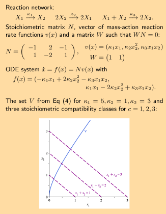
Figure 1: Running example. Example network with two species, $X_{1}$ and $X_{2}$, and three reactions with mass-action kinetics.

The concentrations of the species $X_{1},\dots,X_{n}$ are denoted by lower-case letters $x_{1},\dots,x_{n}$ and we let $x=(x_{1},\ldots,x_{n})$. We denote by $\mathbb{R}^{n}_{>0}$ ($\mathbb{R}^{n}_{\geq 0}$), the positive (non-negative) orthant in $\mathbb{R}^{n}$. The evolution of the concentrations with respect to time is modeled as an ODE system derived from a set of reaction rate functions. A reaction rate function for reaction $R_{j}$ is a $\mathcal{C}^{1}$-function $v_{j}\colon\mathbb{R}_{\geq 0}^{n}\rightarrow\mathbb{R}_{\geq 0}$ that models the (non-negative) speed of the reaction. We further assume that

$$v_{j}(x)=0\quad\Leftrightarrow\quad x_{i}=0\quad\textrm{ for some }i\textrm{ such that }\alpha_{ij}>0,$$ (2)

that is, the reaction only takes place in the presence of all reactant species. We refer to the set of reaction rate functions as the kinetics.

A particular important example of a kinetics is that of mass-action kinetics. In this case the reaction rate functions are given by

$$v_{j}(x)=\kappa_{j}x_{1}^{\alpha_{1j}}\cdot\ldots\cdot x_{n}^{\alpha_{nj}},\qquad j=1,\dots,\ell,$$

where $\kappa_{j}$ is a positive number called the reaction rate constant and we assume $0^{0}=1$. Other important examples are Michaelis-Menten kinetics and Hill kinetics. All three types of kinetics fulfil the assumption in Eq (2).

For a choice of reaction rate functions $v=(v_{1},\ldots,v_{\ell})$, the ODE system modelling the species concentrations over time with initial condition $x(0)=x_{0}$, is

$$\dot{x}=f(x),\qquad x\in\mathbb{R}^{n}_{\geq 0},\qquad\textrm{where }\quad f(x)=Nv(x).$$ (3)

Under assumption Eq (2), the orthants $\mathbb{R}^{n}_{>0}$ and $\mathbb{R}^{n}_{\geq 0}$ are forward-invariant under $f$ in Eq (21) [27, Theorem 5.6], [28, Section 16]. Forward-invariance implies that the solutions to the ODE system stays in $\mathbb{R}^{n}_{>0}$ (resp. $\mathbb{R}^{n}_{\geq 0}$) for all positive times if the initial condition is in $\mathbb{R}^{n}_{>0}$ (resp. $\mathbb{R}^{n}_{\geq 0}$).

The trajectories of the ODEs in Eq (21) are confined to the so-called stoichiometric compatibility classes, which are defined as follows. Let $s=\text{rank}(N)$ be the rank of the network and $d=n-s$ be the corank. Further, let $W\in\mathbb{R}^{d\times n}$ be any matrix of full rank $d$ such that $WN=0$, see Fig 1 for an example. This matrix is zero-dimensional if $N$ has full rank $n$. For each $c\in\mathbb{R}^{d}$, there is an associated stoichiometric compatibility class defined as

$$\mathcal{P}_{c}:=\{x\in\mathbb{R}^{n}_{\geq 0}\mid Wx=c\}.$$

This set is empty if $c\notin W(\mathbb{R}^{n}_{\geq 0})$. The positive stoichiometric compatibility class is defined as the relative interior of $\mathcal{P}_{c}$, that is, the intersection of $\mathcal{P}_{c}$ with the positive orthant:

$$\mathcal{P}_{c}^{+}:=\{x\in\mathbb{R}^{n}_{>0}\mid Wx=c\}=\mathcal{P}_{c}\cap\mathbb{R}^{n}_{>0}.$$

The sets $\mathcal{P}_{c}^{+}$ and $\mathcal{P}_{c}$ are convex. Since by construction $Wx$ is conserved over time and determined by the initial condition, then $\mathcal{P}_{c}^{+}$ and $\mathcal{P}_{c}$ are also forward-invariant.

An equation of the form $\omega\cdot x=c^{\prime}$ for some $\omega\in\operatorname*{im}(N)^{\perp}$ and $c^{\prime}\in\mathbb{R}$ is called a conservation relation. In particular, $Wx=c$ forms a system of $d$ conservation relations.

For the running example in Fig 1, the rank of the network is $s=1$ and the corank is $d=1$. The matrix $W$ in the figure leads to the conservation relation $x_{1}+x_{2}=c$. Here the stoichiometric compatibility class $\mathcal{P}_{c}$ has non-empty interior, that is, $\mathcal{P}_{c}^{+}\neq\emptyset$, if and only if $c>0$.

In the following, to ease the notation, we implicitly assume a reaction network comes with a kinetics (a set of reaction rate functions) and the associated ODE system.

Dissipative and conservative reaction networks.

A reaction network is dissipative if, for all stoichiometric compatibility classes $\mathcal{P}_{c}$, there exists a compact set where the trajectories of $\mathcal{P}_{c}$ eventually enter (see §3.2 in the Supporting Information). A reaction network is conservative if there exists a conservation relation with only positive coefficients, or, equivalently, if for all species $X_{i}$ there is a conservation relation such that the coefficient of $x_{i}$ is positive and all other coefficients are non-negative. This is equivalent to the stoichiometric compatibility classes being compact sets [29]. Hence, in particular, a conservative reaction network is dissipative because we can choose the attracting compact set to be the stoichiometric compatibility class itself. Because of the conservation relation $x_{1}+x_{2}=c$, the reaction network of the running example is conservative.

Equilibria.

Given the ODE in Eq (21), the set of non-negative equilibria is the set of points for which $f(x)$ vanishes:

$$V=\{x\in\mathbb{R}^{n}_{\geq 0}\mid f(x)=0\}.$$ (4)

We are interested in the positive equilibria in each stoichiometric compatibility class, that is, in the set $V\cap{\mathcal{P}_{c}^{+}}$. Generically, this set consists of isolated points obtained as the simultaneous positive solutions to the equations

$$f(x)=0,\qquad Wx=c.$$ (5)

Fig 1 shows a representation of the set $V$ together with examples of stoichiometric compatibility classes for the running example. The figure suggests that the set $V$ intersects each stoichiometric compatibility class in exactly one point.

We introduce some definitions: a network admits multiple equilibria (or is multistationary) if there exists $c\in\mathbb{R}^{d}$ such that $V\cap\mathcal{P}_{c}^{+}$ contains at least two points, that is, the system in Eq (5) has at least two positive solutions. Equilibria belonging to $V\cap\mathcal{P}_{c}$ but not to $V\cap\mathcal{P}_{c}^{+}$ for some $c$ are boundary equilibria. A boundary equilibrium has at least one coordinate equal to zero.

The function $\varphi_{c}(x)$.

Some of the $n$ equations in the system $f(x)=0$ might be redundant. Indeed, every vector $\omega\in\operatorname*{im}(N)^{\perp}$ fulfils $\omega\cdot f(x)=0$, and hence gives a linear relation among the entries of $f(x)$. As a consequence, there are (at least) as many independent linear relations as rows of $W$, that is, $d$, and there are at most $s=n-d$ linearly independent equations in the system $f(x)=0$. Thus $d$ of the equations are redundant. By removing these from $f(x)=0$, the system in Eq (5) becomes a system of $n$ equations in $n$ variables.

In order to systematically choose $d$ equations to remove, we proceed as follows. We choose the matrix of conservation relations $W\in\mathbb{R}^{d\times n}$ to be row reduced and let $i_{1},\dots,i_{d}$ be the indices of the first non-zero coordinate of each row. Then the scalar product of the $j$-th row of $W$ with $f(x)$ can be used to express $f_{i_{j}}(x)$ as a linear combination of the entries of $f(x)$ with indices different from $i_{1},\dots,i_{d}$. It follows that the equations $f_{i_{1}}(x)=0,\dots,f_{i_{d}}(x)=0$ can be removed.

For $c\in\mathbb{R}^{d}$, we define the $\mathcal{C}^{1}$-function $\varphi_{c}(x)\colon\mathbb{R}^{n}_{\geq 0}\rightarrow\mathbb{R}^{n}$ by

$$\varphi_{c}(x)_{i}=\begin{cases}f_{i}(x)&i\notin\{i_{1},\dots,i_{d}\}\\ (Wx-c)_{i}&i\in\{i_{1},\dots,i_{d}\}.\end{cases}$$ (6)

For the running example in Fig 1 the matrix $W$ is already row reduced with $i_{1}=1$. Hence $\varphi_{c}$ is obtained by replacing $f_{1}(x)$ with $x_{1}+x_{2}-c$:

$$\varphi_{c}(x)=\begin{pmatrix}x_{1}+x_{2}-c\\ \kappa_{1}x_{1}-2\kappa_{2}x_{2}^{2}+\kappa_{3}x_{1}x_{2}\end{pmatrix}.$$

As the function $\varphi_{c}(x)$ is obtained by replacing redundant equations in $f(x)=0$ with equations defining $\mathcal{P}_{c}$, we have

$$V\cap\mathcal{P}_{c}=\{x\in\mathbb{R}^{n}_{\geq 0}\mid\varphi_{c}(x)=0\}.$$

Consequently, a network admits multiple equilibria if the equation $\varphi_{c}(x)=0$ has at least two positive solutions for some $c\in\mathbb{R}^{d}$.

A theorem for unique and multiple equilibria.

Let $M(x)\in\mathbb{R}^{n\times n}$ be the Jacobian matrix of $\varphi_{c}(x)$, that is, the matrix with $(i,j)$-th entry equal to the partial derivative of $\varphi_{c,i}(x)$ with respect to $x_{j}$. The matrix $M(x)$ does not depend on $c$, see Eq (6).

We say that an equilibrium $x^{*}\in V\cap\mathcal{P}_{c}$ is non-degenerate if the Jacobian of $\varphi_{c}$ at $x^{*}$, $M(x^{*})$, is non-singular, that is, if $\det(M(x^{*}))\neq 0$ [10].

Theorem 1 (Unique and multiple equilibria). Assume the reaction rate functions fulfil Eq (2), let $s=\text{rank}(N)$ and let $\mathcal{P}_{c}$ be a stoichiometric compatibility class such that $\mathcal{P}_{c}^{+}\neq\emptyset$, where $c\in\mathbb{R}^{d}$. Further, assume that

(i) The network is dissipative.

(ii) There are no boundary equilibria in $\mathcal{P}_{c}$.

Then the following holds.

(A’) Uniqueness of equilibria. If

$$\operatorname*{sign}(\det(M(x)))=(-1)^{s}\quad\textrm{ for {all} positive equilibria}\quad x\in V\cap\mathcal{P}_{c}^{+},$$

then there is exactly one positive equilibrium in $\mathcal{P}_{c}$. Further, this equilibrium is non-degenerate.

(B’) Multiple equilibria. If

$$\operatorname*{sign}(\det(M(x)))=(-1)^{s+1}\quad\text{ for {some} equilibrium }\quad x\in V\cap\mathcal{P}_{c}^{+},$$

then there are at least two positive equilibria in $\mathcal{P}_{c}$, at least one of which is non-degenerate. If all positive equilibria in $\mathcal{P}_{c}$ are non-degenerate, then there are at least three and always an odd number.

The proof of Theorem 1 is based on relating $\det(M(x))$ to the Brouwer degree of $\varphi_{c}$ at $0$ (see §1-§4 in the Supporting Information). Note that the only situation that is not covered by Theorem 1 is when $\operatorname*{sign}(\det(M(x)))$ takes the value $0$ for some $x$, but never the value $(-1)^{s+1}$. The determinant of $M(x)$ is the same as the core determinant in [30, Lemma 3.7]. See also [10, Remark 9.27].

To check whether the sign conditions in part (A’) or (B’) hold requires information about the equilibria in $\mathcal{P}_{c}^{+}$. As such, these conditions are difficult to check. If $\operatorname*{sign}(\det(M(x)))$ is constant for all $x$ in a set containing the positive equilibria, then the condition in (A’) is always fulfilled. In particular, this is the case for injective networks, where $\operatorname*{sign}(\det(M(x)))=(-1)^{s}$ for all $x\in\mathbb{R}^{n}_{>0}$ [10] (see also [31, 32, 33, 34, 35, 36] for related work on injective networks). The latter might be verified or falsified without any knowledge about the equilibria of the system (see the comments to Step 5 and Step 7 in the section “Procedure for finding parameter regions for mono- and multistationarity”).

Corollary 1 (Unique equilibria). Assume that the assumptions of Theorem 1 hold and that $\operatorname*{sign}(\det(M(x)))=(-1)^{s}$ for all $x\in\mathbb{R}^{n}_{>0}$. Then there is exactly one positive equilibrium in each stoichiometric compatibility class. Further, this equilibrium is non-degenerate.

The conclusions of Theorem 1 refer specifically to non-degenerate equilibria. Non-degenerate equilibria are always isolated from each other within a given stoichiometric compatibility class, as $\det(M(x))\not=0$ ensures $M(x)$ is locally invertible. In some situations we might be able to “lift” non-degenerate equilibria of a reaction network to another reaction network that in some sense is larger, thereby proving lower bounds on the number of non-degenerate equilibria of the larger reaction network. This is for example the case if the smaller network is embedded in the larger [37, 38], if the smaller network is without inflows/outflows while the larger has all inflows/outflows [39], or if the smaller is obtained by elimination of intermediate species [40]. Conditions for the existence of degenerate equilibria, where $\det(M(x))$ is expected to change sign, are also known [41, 20].

Positive parameterizations and a corollary.

Verifying condition (A’) or (B’) is considerably easier if there exists a positive parameterization of the set $V\cap\mathbb{R}^{n}_{>0}$ of all positive equilibria. In this subsection we define such a parameterization and restate Theorem 1 as Corollary 2 in this situation. In the following sections this corollary will become the foundation for the procedure to partition the parameter space into regions with different equilibrium properties.

By a positive parameterization of the set of positive equilibria we mean a surjective function

$$\begin{array}[]{rccc}\Phi\colon&\mathbb{R}^{m}_{>0}&\rightarrow&{V\cap}\mathbb{R}^{n}_{>0}\\ &\hat{x}={(\hat{x}_{1},\dots,\hat{x}_{m})}&\mapsto&{(\Phi_{1}(\hat{x}),\dots,\Phi_{n}(\hat{x})),}\end{array}$$ (7)

for some $m<n$, such that $\hat{x}\in\mathbb{R}^{m}_{>0}$ is the vector of free variables. In other words, a positive parameterization implies that $x_{1},\dots,x_{n}$ are expressed at equilibrium as functions of $\hat{x}$:

$$x_{i}=\Phi_{i}(\hat{x}),\qquad i={1},\dots,n,$$

such that $x_{1},\dots,x_{n}$ are positive provided $\hat{x}$ is positive. Thus

$$V\cap\mathbb{R}^{n}_{>0}=\{\Phi(\hat{x})\mid\hat{x}\in\mathbb{R}^{m}_{>0}\}.$$ (8)

Typically, the number of free variables equals the corank of the network, that is $m=d=n-s$.

We say that a parameterization is algebraic if the components $\Phi_{i}(\hat{x})$ are polynomials or rational functions (quotients of polynomials) and can be given such that the denominator is positive for all $\hat{x}$. See Fig 2 (Step 6) for an application to the running example. Note that the parameterizations considered here do not make use of the conservation relations.

A positive equilibrium $\Phi(\hat{x})$, $\hat{x}\in\mathbb{R}^{m}_{>0}$, belongs to the stoichiometric compatibility class $\mathcal{P}_{c}$ where

$$c:=W\Phi(\hat{x}).$$ (9)

Combining Eq (8) and Eq (9), it follows that the positive solutions to Eq (5) for a given $c$ are in one-to-one correspondence with the positive solutions to Eq (9), that is,

$$V\cap\mathcal{P}_{c}^{+}=\{\Phi(\hat{x})\mid\hat{x}\in\mathbb{R}^{m}_{>0}\quad\textrm{and}\quad c=W\Phi(\hat{x})\}.$$

In order to restate Theorem 1 using the parameterization $\Phi$, we consider the determinant of $M(x)$ evaluated at $\Phi(\hat{x})$,

$$a(\hat{x})=\det(M(\Phi(\hat{x}))),\quad\hat{x}\in\mathbb{R}^{m}_{>0}.$$ (10)

Corollary 2 (Positive parameterization). Assume the reaction rate functions fulfil Eq (2) and let $s=\text{rank}(N)$. Further, assume that

(i) The network is dissipative.

(ii) There are no boundary equilibria in $\mathcal{P}_{c}$, for all $c\in\mathbb{R}^{d}$ such that $\mathcal{P}_{c}^{+}\neq\emptyset$.

(iii) The set of positive equilibria admits a positive parameterization as in Eq (27).

Then the following holds.

(A) Uniqueness of equilibria. If

$$\operatorname*{sign}(a(\hat{x}))=(-1)^{s}\quad\textrm{ for {all} }\hat{x}\in\mathbb{R}^{m}_{>0},$$

then there is exactly one positive equilibrium in each $\mathcal{P}_{c}$ with $\mathcal{P}_{c}^{+}\neq\emptyset$. Further, this equilibrium is non-degenerate.

(B) Multiple equilibria. If

$$\operatorname*{sign}(a(\hat{x}))=(-1)^{s+1}\quad\textrm{ for {some} }\hat{x}\in\mathbb{R}^{m}_{>0},$$

then there are at least two positive equilibria in the stoichiometric compatibility class $\mathcal{P}_{c}$ where $c:=W\Phi(\hat{x})$. Further, at least one of the equilibria is non-degenerate. If all positive equilibria in $\mathcal{P}_{c}$ are non-degenerate, then there are at least three equilibria and always an odd number.

Note that, contrary to Theorem 1, the stoichiometric compatibility class $\mathcal{P}_{c}$ is not fixed in the corollary.

In the next section we formulate a procedure based on Corollary 1 and Corollary 2 to find regions of mono- and multistationarity. Before that we end this section with an application to the running example. The analysis is divided into seven steps which prelude the steps of the procedure.

Application of Corollary 1 and Corollary 2 to the running example.

We start with the setup given in Fig 1 and first check whether the sign condition of Corollary 1 is fulfilled, in which case there is a single equilibrium in all stoichiometric compatibility classes. The steps of the analysis are illustrated in Fig 2.

The assumptions of the corollary are easily verified in this case. As we are assuming mass-action kinetics, Eq (2) is fulfilled (Fig 2, Step 1). Further the network is conservative, hence dissipative and (i) is fulfilled (Fig 2, Step 2). It is easily seen that there are no boundary equilibria in any stoichiometric compatibility class with non-empty interior (Fig 2, Step 3). Hence (ii) is fulfilled. We then construct $\varphi_{c}(x)$ and calculate the determinant of $M(x)$. It is a polynomial (in fact, a linear function) in $x_{1},x_{2}$ with coefficients containing both positive and negative terms (Fig 2, Step 4). By choosing $(x_{1},x_{2})\in\mathbb{R}^{2}_{>0}$ with $x_{1}$ large enough, the determinant of $M(x)$ is positive (Fig 2, Step 5). Therefore Corollary 1 cannot be applied as $s=1$. We note that this conclusion is independent of the specific choice of the parameter vector $\kappa=(\kappa_{1},\kappa_{2},\kappa_{3})$, so in fact it holds for all parameter values.

Corollary 2 has the same assumptions as Corollary 1. We find a positive parameterization by solving the equilibrium equation for $x_{1}$. That is, we treat it as an equation in $x_{1}$, while $x_{2}$ $(=\hat{x})$ is treated as a parameter. The function $a(x_{2})$ obtained by substituting $x$ by $\Phi(x_{2})$ in the determinant of $M(x)$ is given in Fig 2, Step 6. It is clear from the expression of $a(x_{2})$ that it takes the sign $-1$ for all $x_{2}>0$. Also this conclusion does not depend on the specific value of $\kappa$. By application of Corollary 2(A) with $s=1$, we conclude that there exists a unique positive non-degenerate equilibrium in each stoichiometric compatibility class with $c>0$, for all values of the reaction rate constants (Fig 2, Step 7). The possibility of multiple equilibria is therefore excluded. In this particular example the existence of a positive parameterization is essential to draw the conclusion.

To illustrate how Corollary 2 can be used to find parameter regions for multistationarity, we consider the polynomial $a(\widehat{x})$ given in the first row of Fig 4, where $n=6$ and $s=4$ (the example is worked out in detail below):

$$a(\widehat{x}) =\frac{1}{{\kappa}_{3}}\big{(}{\kappa}_{2}{\kappa}_{4}{\kappa}_{5}^{2}\mathbf{\left({\kappa}_{1}-{\kappa}_{3}\right)}x_{4}x_{5}^{2}+({\kappa}_{1}+{\kappa}_{2}){\kappa}_{3}{\kappa}_{4}{\kappa}_{5}{\kappa}_{6}{x_{5}^{2}}+2{\kappa}_{1}{\kappa}_{2}{\kappa}_{3}{\kappa}_{4}{\kappa}_{5}{x_{4}x_{5}}$$

$$\quad+{\kappa}_{1}({\kappa}_{2}+{\kappa}_{3}){\kappa}_{3}{\kappa}_{5}{\kappa}_{6}{x_{5}}+{\kappa}_{1}{\kappa}_{2}{\kappa}_{3}^{2}{\kappa}_{5}{x_{4}}+{\kappa}_{1}{\kappa}_{2}{\kappa}_{3}^{2}{\kappa}_{6}\big{)}.$$

Only one of the coefficients of the polynomial $a(\hat{x})$ in $x_{4},x_{5}$ can be negative. If ${\kappa}_{3}\leq{\kappa}_{1}$, then $\operatorname*{sign}(a(\hat{x}))=(-1)^{4}=1$ for all positive $\hat{x}$. Corollary 2(A) implies that there is a unique positive non-degenerate equilibrium in each stoichiometric compatibility class with non-empty positive part.

Oppositely, we show that for ${\kappa}_{3}>{\kappa}_{1}$, Corollary 2(B) applies. For that, let $x_{4}=T$ and $x_{5}=T$. Then $a(\hat{x})$ becomes a polynomial in $T$ with negative leading coefficient of degree $3$. For $T$ large enough, $a(\widehat{x})$ is negative, and we conclude that there exists $\hat{x}$ such that $\operatorname*{sign}(a(\hat{x}))=(-1)^{5}=-1$. Corollary 2(B) implies that there exists a stoichiometric compatibility class $\mathcal{P}_{c}$ that contains at least two positive equilibria. In summary, the region of the parameter space for which multistationarity exists is completely characterized by the inequality ${\kappa}_{3}>{\kappa}_{1}$.

Step 5 and 7 are sign analyses of $\det(M(x))$ and $a(\hat{x})$, respectively. These are crucial steps and essential for determining parameter regions with mono- and multistationarity. In general, the sign of a polynomial might be studied by studying the signs of the coefficients of the monomials in the polynomial. If all coefficients have the same sign, then the polynomial is either positive or negative for all $x\in\mathbb{R}^{n}_{>0}$, respectively, $\hat{x}\in\mathbb{R}^{m}_{>0}$, depending on the sign, and Corollary 1, respectively, Corollary 2(A) applies. If this is not the case, then Corollary 2(B) might be applicable if we can show that the polynomial has the sign $(-1)^{s+1}$ for some $\hat{x}\in\mathbb{R}^{m}_{>0}$. In the two examples discussed here, the signs of $\det(M(x))$ and $a(\hat{x})$ are straightforward to analyse. However, this is not always the case, see the section “Checking the steps of the procedure”.

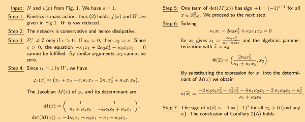
Figure 2: Step 1-3 check the assumptions of Corollary 1 and Corollary 2. In step 4 the function $\varphi_{c}(x)$ is constructed and the determinant of $M(x)$ is found. Step 5 is the sign analysis of the polynomial $\det(M(x))$ for $x\in\mathbb{R}^{2}_{>0}$. Step 6 establishes a positive parameterization and finds the polynomial $a(\hat{x})$. Step 7 is similar to step 5, but for $a(\hat{x})$.

Procedure for finding parameter regions for multistationarity

In the previous subsection we applied Corollary 1 and Corollary 2 to the running example by going through a number of steps corresponding to the conditions of the statements and the calculation of the determinant. In this section we outline the steps formally. Afterwards we discuss the steps and how they can be verified either manually or algorithmically, that is, without user intervention. Finally we devise an algorithm to conclude uniqueness of equilibria or to find regions in the parameter space where multistationarity occurs. We conclude this section with some extra examples that follow the steps of the procedure.

We assume the reaction rate functions $v(x)$ depend on some parameters ${\kappa}$. The reaction rate functions are further assumed to be polynomials (as for mass-action kinetics) or quotients of polynomials (as for Michaelis-Menten and Hill kinetics with integer exponents).

The input to the procedure is $v(x)$ and $N$ (the stoichiometric matrix) and the output is parameter regions for which the network admits multistationarity or uniqueness of equilibria.

Procedure (Identification of parameter regions for multistationarity)

Input: $N$ and $v(x)$ depending on $\kappa$.

1. Find $f(x)$, a row reduced matrix $W$ of size $d\times n$ such that $WN=0$, and check that $v(x)$ vanishes in the absence of one of the reactant species, that is, check that it satisfies Eq (2).

2. Check that the network is dissipative.

3. Check for boundary equilibria in $\mathcal{P}_{c}$ for $\mathcal{P}_{c}^{+}\neq\emptyset$ and $c\in\mathbb{R}^{d}$.

4. Construct $\varphi_{c}(x)$, $M(x)$ and compute $\det(M(x))$.

5. Analyze the sign of $\det(M(x))$. Find conditions on the parameters ${\kappa}$ such that $\operatorname*{sign}(\det(M(x)))=(-1)^{s}$ for all $x\in\mathbb{R}^{n}_{>0}$, in which case Corollary 1 holds.

If Corollary 1 does not hold for all ${\kappa}$, continue to the next step.

6. Obtain an algebraic parameterization $\Phi(\hat{x})$ of the set of positive equilibria for all $\kappa$, as in Eq (27), such that the coefficients of the numerator and the denominator of each $\Phi_{i}(\hat{x})$ possibly depend on $\kappa$. Compute $a(\hat{x})=\det(M(\Phi(\hat{x})))$. By hypothesis, $a(\hat{x})$ can be written as the quotient of two polynomials in $\hat{x}$ with coefficients depending on $\kappa$, whose denominator takes positive values.

7. Analyze the sign of the numerator of $a(\hat{x})$.

7a. Identify coefficients with sign $(-1)^{s+1}$ and coefficients that can have different signs depending on the parameters.

7b. Use the terms corresponding to identified coefficients to construct parameter inequalities such that, whenever these inequalities hold, one has either $\operatorname*{sign}(a(\hat{x}))=(-1)^{s}$ for all $\hat{x}\in\mathbb{R}^{m}_{>0}$ or $\operatorname*{sign}(a(\hat{x}))=(-1)^{s+1}$ for at least one $\hat{x}\in\mathbb{R}^{m}_{>0}$, in which case either Corollary 2(A) or (B) holds.

There is no guarantee that all steps of the procedure can be carried out successfully, let alone automatically. While step 1 and 4 usually are straightforward (only computational issues might arise for large networks), step 2, 3, 5, 6 and 7 might in particular require case specific approaches. However, there exist computationally feasible sufficient criteria that guarantee the conditions in each step can be checked efficiently.

Checking the steps of the procedure.

Step 2: establishing dissipativity.

If the network is not dissipative, then at least one concentration grows to infinity over time. This is typically not the case for realistic networks, but it needs to be ruled out in order to apply the procedure.

We start by checking whether the network is conservative. This implies solving the linear system $\omega^{t}\,N=0$ with the constraint $\omega>0$. Alternatively, conservation relations are often easily established by inspection of the reactions. For example, in many signalling networks, the total concentration of enzyme (free and bounded) and of substrate (phosphoforms) are conserved.

If the network is not conservative, then we check whether it is strongly endotactic [42, 43]. Strongly endotactic reaction networks are in particular permanent, that is, dissipative and the compact set can be chosen such that it does not intersect the boundary of $\mathbb{R}_{>0}^{n}$, see [42, 43, 44] for details.

If the network is neither conservative nor strongly endotactic, then we can use the following proposition to decide on dissipativity (see the §3.2 in the Supporting Information).

Proposition 1 (Dissipative network). Let $||\cdot||$ be a norm in $\mathbb{R}^{n}$. Assume that for each $c$ with $\mathcal{P}_{c}^{+}\neq\emptyset$, there exists a vector $\omega_{c}\in\mathbb{R}^{n}_{>0}$ and a number $R>0$ such that $\omega_{c}\cdot f(x)<0$ for all $x\in\mathcal{P}_{c}$ with $||x||>R$. Then the network is dissipative.

Thus, we look for vectors $\omega_{c}$ with all coordinates positive and such that $\omega_{c}\cdot f(x)<0$ for large $x$. To avoid restricting the parameter values, this computation should be done symbolically.

Step 3: absence of boundary equilibria.

For systems of moderate size it is often possible to establish nonexistence of boundary equilibria by arguments similar to those employed in the analysis of the running example: for each $i$, assume $x_{i}=0$, and show that it leads to a contradiction.

A systematic procedure to check for the existence of boundary equilibria relies on computing the so-called minimal siphons of the network [45]. A siphon is a set of species $Z\subseteq\{X_{1},\dots,X_{n}\}$ fulfilling the following closure property: if $X_{i}\in Z$ and $X_{i}$ is produced in reaction $R_{j}$ (that is, $\beta_{ij}>0$), then there exists $X_{k}\in Z$ such that $X_{k}$ is consumed in the same reaction (that is, $\alpha_{kj}>0$). A minimal siphon is a siphon that does not properly contain any other siphon.

Proposition 2 (Siphons) ([46, 47]) If for every minimal siphon $Z$ there exists a subset $\{X_{i_{1}},\dots,X_{i_{k}}\}\subseteq Z$, and a conservation relation $\lambda_{1}x_{i_{1}}+\dots+\lambda_{k}x_{i_{k}}=c$ for some positive $\lambda_{1},\dots,\lambda_{k}$, then the network has no boundary equilibria in any stoichiometric compatibility class $\mathcal{P}_{c}$ with $\mathcal{P}_{c}^{+}\neq\emptyset$.

The hypothesis of the proposition can be summarised by saying that each minimal siphon contains the support of a positive conservation relation.

For example, the running example has only one minimal siphon, namely $\{X_{1},X_{2}\}$. The conservation relation $x_{1}+x_{2}=c$ fulfils the requirement of Proposition 2, and hence the network has no boundary equilibria in any $\mathcal{P}_{c}$ with $c>0$.

More information about using siphons to preclude boundary equilibria is given in the section “Computational issues” below and in §5.1 of the Supporting Information.

Step 5: determining the sign of $\det(M(x))$.

If the kinetics is mass-action, then $\det(M(x))$ is a polynomial in $x$. In general, if the reaction rate functions are rational functions in $x$, then so is $\det(M(x))$. In the latter case, if the $j$th reaction rate function fulfils $v_{j}(x)=p_{j}(x)/q_{j}(x)$ with $p_{j}(x)\geq 0$ and $q_{j}(x)>0$ for all $x\in\mathbb{R}^{n}_{>0}$, then $\det(M(x))=p(x)/q(x)$, where $q(x)=\prod_{j=1}^{\ell}q_{j}(x)^{2}>0$. It follows from the definition of $M(x)$ and by differentiation of $v_{j}(x)$, $j=1,\ldots,\ell$.

We determine conditions on the parameters such that all coefficients of $p(x)$ have sign $(-1)^{s}$. Then the sign of $\det(M(x))$ is also $(-1)^{s}$ for all $x\in\mathbb{R}^{n}_{>0}$ and Corollary 1 holds.

Step 6: finding an algebraic positive parameterization.

Computer algebra systems like Maple or Mathematica can be used to find a parameterization. One strategy is to solve the equations $f_{i}(x)=0$, $i\notin\{i_{1},\dots,i_{d}\}$, for some subset of (at most) $s$ variables, treating the remaining (at least) $d$ variables as coefficients of the system. If a parameterization found in this way exists but is not positive, another set of variables should be tried out. This can be systematically addressed by trying out all possible subsets of variables. It requires computation and analysis of at most $\left(\begin{smallmatrix}n\\ d\end{smallmatrix}\right)$ parameterizations. Alternatively, one can compute the circuits of degree one of the matroid associated with the equilibrium equations [48].

In some cases, the network structure implies that a positive parameterization of the set of equilibria exists. A set, say $\{X_{k+1},\dots,X_{n}\}$ with $n-k$ elements for some $k$, is non-interacting if two species never appear on the same side of a reaction and they have coefficient at most one in all reactions. In this case the equilibrium equations $f_{k+1}(x)=\dots=f_{n}(x)=0$ form a linear system in the variables $\{x_{k+1},\dots,x_{n}\}$. Provided that the determinant of the coefficient matrix of the linear system is not identically zero, this system can be solved and we obtain a positive parameterization of the non-interacting variables $x_{k+1},\dots,x_{n}$ at equilibrium in terms of the remaining variables $x_{1},\dots,x_{k}$ [49, 50]. A necessary condition for the determinant of the coefficient matrix not being identically zero is that there is no conservation relation of the form $x_{i_{1}}+\dots+x_{i_{l}}$ with $i_{1},\dots,i_{l}\in\{k+1,\dots,n\}$. If a non-interacting set with $k=d$ exists, that is, with $s=n-d$ elements, then this guarantees the existence of the desired parameterization. In the running example there is not a non-interacting set because both species have coefficient $2$ in the reaction $2X_{1}\rightarrow 2X_{2}$.

The non-interacting condition can be relaxed in some cases by requiring that none of the species in $\{X_{k+1},\dots,X_{n}\}$ appear together in a reactant (these sets are called reactant-non-interacting [51]). Proceeding as above, provided that the determinant of the coefficient matrix is not identically zero, $x_{k+1},\dots,x_{n}$ can be expressed at equilibrium in terms of $x_{1},\dots,x_{k}$. Conditions that ensure this is a positive parameterization are given in [51]. In the running example, species $X_{1}$ is a reactant-non-interacting set and we can obtain a positive parameterization of $x_{1}$ in terms of $x_{2}$, see Fig 1 and Fig 2.

If the network admits so-called toric steady states, then a positive parameterization also exists [11].

Step 7: the sign of $a(\hat{x})$ and the Newton polytope.

This is perhaps the hardest step of all. We write $a(\hat{x})=p(\hat{x})/q(\hat{x})$ with $q(\hat{x})$ positive for all $\hat{x}$ and would like to determine the sign of $p(\hat{x})$. We first look for conditions that ensure uniqueness of positive equilibria by imposing that all coefficients of $p(\hat{x})$ as a polynomial in $\hat{x}$ have sign $(-1)^{s}$.

We next identify the monomials of $p(\hat{x})$, where the sign of the coefficient, say $\beta$, is $(-1)^{s+1}$ for some parameter values. For each of these monomials we check whether the monomial can “dominate” the sign of $p(\hat{x})$. That is to say, if $\operatorname*{sign}(\beta)=(-1)^{s+1}$, then we determine whether there is an $\hat{x}$ such that $p(\hat{x})$ also has the sign $(-1)^{s+1}$. If it is the case, then the condition $\operatorname*{sign}(\beta)=(-1)^{s+1}$ is a sufficient condition for multiple equilibria according to Corollary 2(B).

Given a coefficient of a monomial with sign $(-1)^{s+1}$, it might not be straightforward to decide if the polynomial $p(\hat{x})$ has the same sign for some value of $\hat{x}$. (For example, the polynomial $x^{2}-2xy+y^{2}=(x-y)^{2}$ has one monomial with negative sign, but the polynomial itself can never be negative.) When the number of variables is small, one can attempt to decide the sign as we did in the examples above. Otherwise, our strategy is to determine whether the monomial of interest corresponds to a vertex of the Newton polytope. If that is the case, then the monomial can dominate the sign of $p(\hat{x})$ (see $\S$5.2 in the Supporting Information). The Newton polytope of $p(\hat{x})$ is defined as the convex hull of the exponent vectors $\alpha=(\alpha_{1},\dots,\alpha_{m})\in\mathbb{R}^{m}$ corresponding to the monomials $\hat{x}_{1}^{\alpha_{1}}\cdot\ldots\cdot\hat{x}_{m}^{\alpha_{m}}$ of $p(\hat{x})$. If $\alpha$ is a vertex of the Newton polytope, then there exists $\hat{x}\in\mathbb{R}^{m}_{>0}$ such that the sign of $p(\hat{x})$ agrees with the sign of the coefficient of the monomial (see $\S$5.2 in the Supporting Information).

Fig 4 shows the Newton polytopes associated with the polynomials in the figure. The vertex corresponding to the monomial of interest is shown in red.

An algorithm.

In the previous subsection we have outlined computational criteria that might be used to verify the conditions of the steps in the procedure. These computational criteria are only sufficient, that is, even if they fail the procedure might still work on the given network. For example, a sufficient computational criterion for the absence of boundary equilibria is based on Proposition 2. However, it might happen that Proposition 2 cannot be applied, but that the network nonetheless has no boundary equilibria in stoichiometric compatibility classes with non-empty interior.

We have collected sufficient computational criteria that guarantee the conditions of the procedure are fulfilled. In this way the procedure is formulated as an algorithm with decision diagram shown in Fig 3. If one step of the algorithm fails, then we say that the algorithm ends indecisively. In that case we might check whether the step can be verified by other means.

For simplicity, we have restricted to mass-action kinetics. Under this assumption, $\det(M(x))$ is a polynomial in $x$ and the parameters ${\kappa}$, and $a(\hat{x})$ is a rational function in $\hat{x}$ and ${\kappa}$ because the parameterization is assumed to be algebraic.

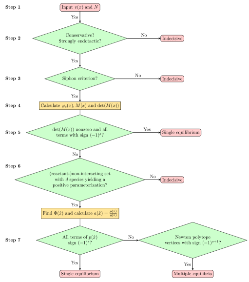
Figure 3: Decision diagram of the algorithm. At each step either the condition is fulfilled or the algorithm terminates indecisively. If that is the case, the corresponding condition might still be verified manually and the algorithm resumed from the next following step.

Applications to selected examples

To illustrate several aspects of the algorithm we provide a detailed step-by-step analysis of a collection of examples.

Two-component system

We have chosen this example to illustrate the situation where an algebraic parameterization is not required, as already $\det(M(x))$ is of constant sign. The algorithm therefore stops successfully at Step 5 (and consequently skips Step 6 and 7).

We consider a simple version of a two-component system consisting of a histidine kinase HK that autophosphorylates and transfers the phosphate group to a response regulator RR, which undergoes autodephosphorylation. The reactions of the network are

$${\rm HK} \cee{->[{\kappa}_{1}]}{\rm HK}_{p} {\rm HK}_{p}+{\rm RR} \cee{->[{\kappa}_{2}]}{\rm HK}+{\rm RR}_{p} {\rm RR}_{p} \cee{->[{\kappa}_{3}]}{\rm RR}.$$

We let $X_{1}={\rm HK}$, $X_{2}={\rm HK}_{p}$, $X_{3}={\rm RR}$ and $X_{4}={\rm RR}_{p}$. The stoichiometric matrix $N$ and a row reduced matrix $W$ such that $WN=0$ are

$$N=\left(\begin{array}[]{rrrr}-1&1&0\\ 1&-1&0\\ 0&-1&1\\ 0&1&-1\end{array}\right),\qquad W=\begin{pmatrix}1&1&0&0\\ 0&0&1&1\end{pmatrix}.$$

The matrix $W$ gives rise to the conservation relations $x_{1}+x_{2}=c_{1}$ and $x_{3}+x_{4}=c_{2}$. With mass-action kinetics, the vector of reaction rates is $v(x)=(\kappa_{1}x_{1},\kappa_{2}x_{2}x_{3},\kappa_{3}x_{4}),$ and the function $f(x)=Nv(x)$ is

$$f(x) =(-\kappa_{1}x_{1}+\kappa_{2}x_{2}x_{3},\kappa_{1}x_{1}-\kappa_{2}x_{2}x_{3}-\kappa_{2}x_{2}x_{3}+\kappa_{3}x_{4},\kappa_{2}x_{2}x_{3}-\kappa_{3}x_{4}).$$

We apply the algorithm to this network.

Step 1. Mass-action kinetics fulfills assumption in Eq (2) on the vanishing of reaction rate functions. The function $f(x)$ and $W$ are given above. The matrix $W$ is row reduced.

Step 2. The network is conservative since $(1,1,1,1)\in\operatorname*{im}(N)^{\perp}$. Therefore the network is dissipative.

Step 3. The minimal siphons of the network are $\{X_{1},X_{2}\}$ and $\{X_{3},X_{4}\}$. These two sets are the supports of the conservation relations. By Proposition 2, there are no boundary equilibria in any $\mathcal{P}_{c}$ as long as $\mathcal{P}_{c}^{+}\neq\emptyset$.

Step 4. With our choice of $W$, we have $i_{1}=1,i_{2}=3$. Hence $\varphi_{c}$ is obtained by replacing the components $f_{1}(x),f_{3}(x)$ of $f(x)$ by the expressions derived from the two conservation relations:

$$\varphi_{c}(x) =\bigl{(}x_{1}+x_{2}-c_{1},{\kappa}_{1}x_{1}-{\kappa}_{2}x_{2}x_{3},x_{3}+x_{4}-c_{2},{\kappa}_{2}x_{2}x_{3}-{\kappa}_{3}x_{4}\bigr{)}.$$

The Jacobian $M(x)$ of $\varphi_{c}$ and its determinant are

$$M(x) =\left(\begin{array}[]{cccc}1&1&0&0\\ {\kappa}_{1}&-{\kappa}_{2}x_{3}&-{\kappa}_{2}x_{2}&0\\  0&0&1&1\\ 0&{\kappa}_{2}x_{3}&{\kappa}_{2}x_{2}&-{\kappa}_{3}\end{array}\right).$$

$$\det(M(x)) ={\kappa}_{1}{\kappa}_{2}x_{2}+{\kappa}_{2}{\kappa}_{3}x_{3}+{\kappa}_{1}{\kappa}_{3}.$$

Step 5. All terms of $\det(M(x))$ have sign $+1=(-1)^{s}$, since $s=2$, and thus the conclusion of Corollary 1 holds. The network admits exactly one non-degenerate equilibrium point in every stoichiometric compatibility class with non-empty positive part.

Hybrid histidine kinase

This example has been analysed in [52]. Taken with mass-action kinetics the network is known to be multistationary for specific choices of reaction rate constants. We have chosen this example to illustrate how the algorithm can be used to sharpen known results: not only does it establish multistationarity for some parameter values, it provides precise conditions for when it occurs and allows a complete partition of the parameter space into regions with and without multistationarity. It also illustrates the use of an algebraic parameterization, which can be obtained by identifying sets of reactant-non-interacting species, and the use of the Newton polytope in Step 7.

This reaction network is an extension of the two-component system discussed above and it is given in the first row of Fig 4. Specifically, the histidine kinase is assumed to be hybrid, that is, it has two ordered phosphorylation sites [52]. Whenever the second phosphorylation site is occupied, the phosphate group can be transferred to a response protein.

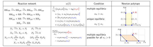
Figure 4: Two examples describing a hybrid histidine kinase (row 1) and a gene transcription network (row 2). Column 1: the reaction network; Column 2: the function $a(\hat{x})$ where monomials with coefficients of constant sign $(-1)^{s}$ are in black, and those that can have sign $(-1)^{s+1}$ are in red; Column 3: parameter conditions for multistationarity; Column 4: Newton polytope where each point corresponds to the exponent vector of a monomial of the numerator of $a(\hat{x})$ (e.g. $(1,2)$ is the exponent vector of the monomial $x_{4}x_{5}^{2}$), black points are the vertices of the Newton polytope and red numbers indicate the exponents of the red monomials in column 2.

Using the notation $X_{1}={\rm HK}_{00}$, $X_{2}={\rm HK}_{p0}$, $X_{3}={\rm HK}_{0p}$, $X_{4}={\rm HK}_{pp}$, $X_{5}={\rm RR}$ and $X_{6}={\rm RR}_{p}$, the stoichiometric matrix $N$ and a row reduced matrix $W$ such that $WN=0$ are

$$N=\left(\begin{array}[]{rrrrrr}-1&0&0&1&0&0\\ 1&-1&0&0&1&0\\ 0&1&-1&-1&0&0\\ 0&0&1&0&-1&0\\ 0&0&0&-1&-1&1\\ 0&0&0&1&1&-1\end{array}\right),\qquad W=\left(\begin{array}[]{rrrrrr}1&1&1&1&0&0\\ 0&0&0&0&1&1\end{array}\right).$$

The matrix $W$ gives rise to the conservation relations $x_{1}+x_{2}+x_{3}+x_{4}=c_{1}$ and $x_{5}+x_{6}=c_{2}.$ We assume mass-action kinetics

$$v(x)=({\kappa}_{1}x_{1},{\kappa}_{2}x_{2},{\kappa}_{3}x_{3},{\kappa}_{4}x_{3}x_{5},{\kappa}_{5}x_{4}x_{5},{\kappa}_{6}x_{6}),$$

and the function is

$$f(x) =(-\kappa_{1}x_{1}+\kappa_{4}x_{3}x_{5},\kappa_{1}x_{1}-\kappa_{2}x_{2}+\kappa_{5}x_{4}x_{5},-\kappa_{3}x_{3}+\kappa_{2}x_{2}-\kappa_{4}x_{3}x_{5},$$

$$\qquad\kappa_{3}x_{3}-\kappa_{5}x_{4}x_{5},-\kappa_{4}x_{3}x_{5}-\kappa_{5}x_{4}x_{5}+\kappa_{6}x_{6},\kappa_{4}x_{3}x_{5}-\kappa_{6}x_{6}+\kappa_{5}x_{4}x_{5}).$$

We apply the algorithm to this network.

Step 1. Mass-action kinetics fulfills assumption in Eq (2) on the vanishing of reaction rate functions. The function $f(x)$ and $W$ are given above. The matrix $W$ is row reduced.

Step 2. Since $(1,1,1,1,1,1)\in\operatorname*{im}(N)^{\perp}$ the network is conservative and hence dissipative.

Step 3. The network has two minimal siphons $\{X_{1},X_{2},X_{3},X_{4}\}$ and $\{X_{5},X_{6}\}$, which are respectively the supports of the two conservation relations. We apply Proposition 2 to conclude that there are no boundary equilibria in any $\mathcal{P}_{c}$ as long as $\mathcal{P}_{c}^{+}\neq\emptyset$.

Step 4. Since $i_{1}=1,i_{2}=5$, the function $\varphi_{c}$ is obtained by replacing the components $f_{1}(x),f_{5}(x)$ of $f(x)$ by the expressions derived from the two conservation relations:

$$\varphi_{c}(x) =(x_{1}+x_{2}+x_{3}+x_{4}-c_{1},\kappa_{1}x_{1}-\kappa_{2}x_{2}+\kappa_{5}x_{4}x_{5},-\kappa_{3}x_{3}+\kappa_{2}x_{2}-\kappa_{4}x_{3}x_{5},$$

$$\qquad\kappa_{3}x_{3}-\kappa_{5}x_{4}x_{5},x_{5}+x_{6}-c_{2},\kappa_{4}x_{3}x_{5}-\kappa_{6}x_{6}+\kappa_{5}x_{4}x_{5}).$$

The Jacobian $M(x)$ of $\varphi_{c}(x)$ and its determinant are

$$M(x) =\left(\begin{array}[]{cccccc}1&1&1&1&0&0\\ {\kappa}_{1}&-{\kappa}_{2}&0&{\kappa}_{5}x_{5}&{\kappa}_{5}x_{4}&0\\ 0&{\kappa}_{2}&-{\kappa}_{3}-{\kappa}_{4}x_{5}&0&-{\kappa}_{4}x_{3}&0\\ 0&0&{\kappa}_{3}&-{\kappa}_{5}x_{5}&-{\kappa}_{5}x_{4}&0\\ 0&0&0&0&1&1\\ 0&0&{\kappa}_{4}x_{5}&{\kappa}_{5}x_{5}&{\kappa}_{4}x_{3}+{\kappa}_{5}x_{4}&-{\kappa}_{6}\end{array}\right),$$

$$\det(M(x)) =\kappa_{2}\kappa_{4}\kappa_{5}(\kappa_{1}-\kappa_{3})x_{3}x_{5}+\kappa_{1}\kappa_{2}\kappa_{4}\kappa_{5}x_{4}x_{5}+\kappa_{4}\kappa_{5}\kappa_{6}(\kappa_{1}+\kappa_{2})x_{5}^{2}$$

$$\quad+\kappa_{1}\kappa_{2}\kappa_{3}\kappa_{4}x_{3}+\kappa_{1}\kappa_{2}\kappa_{3}\kappa_{5}x_{4}+\kappa_{1}\kappa_{5}\kappa_{6}(\kappa_{3}+\kappa_{2})x_{5}+\kappa_{1}\kappa_{2}\kappa_{3}\kappa_{6}.$$

Step 5. The sign of the first coefficient of $\det(M(x))$ depends on the parameters. If $\kappa_{1}\geq\kappa_{3}$, then the sign is positive and $\det(M(x))$ has sign $+1=(-1)^{4}$ ($s=4$) as the remaining terms are positive. According to Corollary 1, there is a single non-degenerate equilibrium in each stoichiometric compatibility class with non-empty positive part. If $\kappa_{1}<\kappa_{3}$, then Corollary 1 cannot be applied. We proceed to the next step to investigate the parameter space further.

Step 6. The set $\{X_{1},X_{2},X_{3},X_{6}\}$ is reactant-non-interacting and consists of $s=4$ elements. We solve the equilibrium equations $f_{1}=f_{2}=f_{3}=f_{6}=0$ for $x_{1},x_{2},x_{3},x_{6}$. This gives the following algebraic parameterization $\Phi\colon\mathbb{R}^{2}_{>0}\rightarrow{V\cap}\mathbb{R}^{6}_{>0}$ of the set of equilibria in terms of $\widehat{x}=(x_{4},x_{5})$:

$$\Phi(x_{4},x_{5}) =\Big{(}\frac{{\kappa}_{4}{\kappa}_{5}x_{4}x_{5}^{2}}{{\kappa}_{1}{\kappa}_{3}},\frac{{\kappa}_{5}({\kappa}_{4}x_{5}+{\kappa}_{3})x_{4}x_{5}}{{\kappa}_{2}{\kappa}_{3}},\frac{{\kappa}_{5}x_{4}x_{5}}{{\kappa}_{3}},x_{4},x_{5},\frac{{\kappa}_{5}({\kappa}_{4}x_{5}+{\kappa}_{3})x_{4}x_{5}}{{\kappa}_{3}{\kappa}_{6}}\Big{)}.$$

The function $a(\hat{x})$, which is $\det(M(x))$ evaluated at $\Phi(x_{4},x_{5})$, is the polynomial given in the first row of Fig 4.

Step 7. We assume $\kappa_{1}<\kappa_{3}$, as the case $\kappa_{1}\geq\kappa_{3}$ is analysed in Step 5. Only one coefficient of $a(\hat{x})$ has sign $-1=(-1)^{s+1}=(-1)^{5}$. The monomial associated with this term is $x_{4}x_{5}^{2}$. As the point $(1,2)$ (the degrees of the monomial) is a vertex of the Newton polytope (see Fig 4), then there exists $\hat{x}\in\mathbb{R}^{m}_{>0}$ such that the sign of $a(\hat{x})$ is $-1$. Corollary 2(B) implies that there exists $c=(c_{1},c_{2})$ such that $\mathcal{P}_{c}$ contains at least two positive equilibria.

Multistationarity is thus completely characterized by the inequality ${\kappa}_{3}>{\kappa}_{1}$. This condition states that the reaction rate constant for phosphorylation of the first site of the hybrid kinase is larger if the second site is phosphorylated than if it is not.

Gene transcription network

We consider the gene transcription network given in row 2 of Fig 4. This example has been studied in [53]. The particularities of this example are that the network is dissipative but not conservative, and that it displays multistationarity for all parameters $\kappa$. Further, this network illustrates the situation where the algorithm stops inconclusively at some step, but can be resumed after successful manual verification.

The network represents a gene transcription motif with two proteins $P_{1},P_{2}$, produced by their respective genes $X_{1},X_{2}$, and such that $P_{2}$ dimerises [53]. Further, the proteins cross regulate each other as depicted in Fig 4. Using the notation $X_{1}=X_{1}$, $X_{2}=X_{2}$, $X_{3}=P_{1}$, $X_{4}=P_{2}$, $X_{5}=X_{2}P_{1}$, $X_{6}=P_{2}P_{2}$, and $X_{7}=X_{1}P_{2}P_{2}$ the stoichiometric matrix $N$ and a row reduced matrix $W$ such that $WN=0$ are

$$\begin{split}N&=\left(\begin{array}[]{rrrrrrrrrr}0&0&0&0&0&0&0&0&-1&1\\ 0&0&0&0&-1&1&0&0&0&0\\ 1&0&-1&0&-1&1&0&0&0&0\\ 0&1&0&-1&0&0&-2&2&0&0\\ 0&0&0&0&1&-1&0&0&0&0\\ 0&0&0&0&0&0&1&-1&-1&1\\ 0&0&0&0&0&0&0&0&1&-1\end{array}\right),\\ W&=\left(\begin{array}[]{rrrrrrr}1&0&0&0&0&0&1\\ 0&1&0&0&1&0&0\end{array}\right).\end{split}$$

From $W$ we find the conservation relations $x_{1}+x_{7}=c_{1}$ and $x_{2}+x_{5}=c_{2}$. Here $s=5$. We consider mass-action kinetics such that

$$v(x)=({\kappa}_{1}x_{1},{\kappa}_{2}x_{2},{\kappa}_{3}x_{3},{\kappa}_{4}x_{4},{\kappa}_{5}x_{2}x_{3},{\kappa}_{6}x_{5},{\kappa}_{7}x_{4}^{2},{\kappa}_{8}x_{6},{\kappa}_{9}x_{1}x_{6},{\kappa}_{10}x_{7})$$

and $f(x)=Nv(x)$ is the function

$$(-{\kappa}_{9}x_{1}x_{6}+{\kappa}_{10}x_{7},-{\kappa}_{5}x_{2}x_{3}+{\kappa}_{6}x_{5},{\kappa}_{1}x_{1}-{\kappa}_{3}x_{3}-{\kappa}_{5}x_{2}x_{3}+{\kappa}_{6}x_{5},{\kappa}_{2}x_{2}-{\kappa}_{4}x_{4}$$

$$\quad-2{\kappa}_{7}x_{4}^{2}+2{\kappa}_{8}x_{6},{\kappa}_{5}x_{2}x_{3}-{\kappa}_{6}x_{5},{\kappa}_{7}x_{4}^{2}-{\kappa}_{8}x_{6}-{\kappa}_{9}x_{1}x_{6}+{\kappa}_{10}x_{7},{\kappa}_{9}x_{1}x_{6}-{\kappa}_{10}x_{7}).$$

We apply the algorithm to this network:

Step 1. Mass-action kinetics fulfills assumption in Eq (2) on the vanishing of reaction rate functions. The function $f(x)$ and $W$ are given above. The matrix $W$ is row reduced.

Step 2. The network is neither conservative nor strongly endotactic. Thus the algorithm terminates inconclusive. We take a manual approach: we pick $\omega_{c}=(1,1,1,1,2,2,3)\in\mathbb{R}^{7}_{>0}$ and observe

$$\omega_{c}\cdot f(x)={\kappa}_{1}x_{1}+{\kappa}_{2}x_{2}-{\kappa}_{3}x_{3}-{\kappa}_{4}x_{4}.$$

Note that $x_{1},x_{2}$ are bounded (due to the conservation relations) while $x_{3},x_{4}$ can be arbitrarily large. Then, for $x_{3},x_{4}$ large enough, $\omega_{c}\cdot f(x)<0$ and the network is dissipative by Proposition 1 (as has been shown in [53] by other means).

Step 3. This network has two minimal siphons: $\{X_{1},X_{7}\}$ and $\{X_{2},X_{5}\}$, which are the supports of the two conservation relations. Therefore, by Proposition 2, there are no boundary steady states in stoichiometric compatibility class with non-empty positive part.

In section §5.1 in the Supporting Information we illustrate how to apply a simplification technique, based on the removal of so-called intermediates and catalysts, to check whether Proposition 2 holds for this network.

Step 4. Using that $i_{1}=1,i_{2}=2$ for our choice of $W$, the function $\varphi_{c}(x)$ is:

$$(x_{1}+x_{7}-c_{1},x_{2}+x_{5}-c_{2},{\kappa}_{1}x_{1}-{\kappa}_{3}x_{3},-{\kappa}_{5}x_{2}x_{3}+{\kappa}_{6}x_{5}{\kappa}_{2}x_{2}-{\kappa}_{4}x_{4}$$

$$\quad-2{\kappa}_{7}x_{4}^{2}+2{\kappa}_{8}x_{6},{\kappa}_{5}x_{2}x_{3}-{\kappa}_{6}x_{5},{\kappa}_{7}x_{4}^{2}-{\kappa}_{8}x_{6}-{\kappa}_{9}x_{1}x_{6}+{\kappa}_{10}x_{7},{\kappa}_{9}x_{1}x_{6}-{\kappa}_{10}x_{7}).$$

The matrix $M(x)$ and its determinant are:

$$M(x) ={\small\left(\begin{array}[]{ccccccc}1&0&0&0&0&0&1\\ 0&1&0&0&1&0&0\\ {\kappa}_{{1}}&-{\kappa}_{{5}}x_{{3}}&-{\kappa}_{{5}}x_{{2}}-{\kappa}_{{3}}&0&{\kappa}_{{6}}&0&0\\ 0&{\kappa}_{{2}}&0&-4{\kappa}_{{7}}x_{{4}}-{\kappa}_{{4}}&0&2{\kappa}_{{8}}&0\\ 0&{\kappa}_{{5}}x_{{3}}&{\kappa}_{{5}}x_{{2}}&0&-{\kappa}_{{6}}&0&0\\ -{\kappa}_{{9}}x_{{6}}&0&0&2\,{\kappa}_{{7}}x_{{4}}&0&-{\kappa}_{{9}}x_{{1}}-{\kappa}_{{8}}&{\kappa}_{{10}}\\ {\kappa}_{{9}}x_{{6}}&0&0&0&0&{\kappa}_{{9}}x_{{1}}&-{\kappa}_{{10}}\end{array}\right),}$$

$$\det(M(x)) =2{\kappa}_{1}{\kappa}_{2}{\kappa}_{5}{\kappa}_{7}{\kappa}_{9}x_{1}x_{2}x_{4}-{\kappa}_{{3}}{\kappa}_{{4}}{\kappa}_{{5}}{\kappa}_{{8}}{\kappa}_{{9}}x_{{3}}x_{{6}}-{\kappa}_{{3}}{\kappa}_{{4}}{\kappa}_{{5}}{\kappa}_{{8}}{\kappa}_{{10}}x_{{3}}$$

$$\qquad-{\kappa}_{{3}}{\kappa}_{{4}}{\kappa}_{{6}}{\kappa}_{{8}}{\kappa}_{{9}}x_{{6}}-{\kappa}_{{3}}{\kappa}_{{4}}{\kappa}_{{6}}{\kappa}_{{8}}{\kappa}_{{10}}.$$

Step 5. One coefficient of $\det(M(x))$ has sign $(-1)^{s+1}=1$ for all values of ${\kappa}$. Thus we proceed to the next step.

Step 6. There is not a set of non-interacting species nor reactant-non-interacting with $s=5$ elements. Thus the algorithm terminates inconclusively.

We take a manual approach and solve the equilibrium equations $f_{3}=f_{4}=f_{5}=f_{6}=f_{7}=0$ for $x_{1},x_{2},x_{3},x_{6},x_{7}$. This gives the following algebraic parameterization $\Phi\colon\mathbb{R}^{2}_{>0}\rightarrow\mathbb{R}^{7}_{>0}$ of the set of equilibria in terms of $\widehat{x}=(x_{4},x_{5})$:

$$\Phi(x_{4},x_{5})=\Big{(}\frac{{\kappa}_{2}{\kappa}_{3}{\kappa}_{6}x_{5}}{{\kappa}_{1}{\kappa}_{4}{\kappa}_{5}x_{4}},\frac{{\kappa}_{4}x_{4}}{{\kappa}_{2}},\frac{{\kappa}_{2}{\kappa}_{6}x_{5}}{{\kappa}_{4}{\kappa}_{5}x_{4}},x_{4},x_{5},\frac{{\kappa}_{7}x_{4}^{2}}{{\kappa}_{8}},\frac{{\kappa}_{2}{\kappa}_{3}{\kappa}_{6}{\kappa}_{7}{\kappa}_{9}x_{4}x_{5}}{{\kappa}_{1}{\kappa}_{4}{\kappa}_{5}{\kappa}_{8}{\kappa}_{10}}\Big{)}.$$

Evaluating $\det(M(x))$ at $\Phi(x_{4},x_{5})$ we obtain the polynomial

$$a(x_{4},x_{5}) =\frac{{\kappa}_{3}{\kappa}_{6}}{x_{4}}({\kappa}_{2}{\kappa}_{7}{\kappa}_{9}x_{4}^{2}x_{5}-{\kappa}_{4}{\kappa}_{7}{\kappa}_{9}x_{4}^{3}-{\kappa}_{2}{\kappa}_{8}{\kappa}_{10}x_{5}-{\kappa}_{4}{\kappa}_{8}{\kappa}_{10}x_{4}).$$

Step 7. The coefficient of the monomial $x_{4}^{2}x_{5}$ of the numerator of $a(x_{4},x_{5})$ has sign $(-1)^{s+1}=(-1)^{6}=1$. Since the monomial $x_{4}^{2}x_{5}$ is a vertex of the associated Newton polytope (see Fig 4), there exists $(x_{4},x_{5})\in\mathbb{R}^{2}_{>0}$ such that the sign of $a(x_{4},x_{5})$ is $1$. We conclude from Corollary 2(B) that for all ${\kappa}_{i}>0$ there exists $c$ such that $\mathcal{P}_{c}$ contains at least two positive equilibria.

Special classes of networks

There are several classes of networks for which some of the steps of the procedure are automatically fulfilled. We review some of them here.

Post-Translational Modification (PTM) networks consist of enzymes ($E_{i}$), substrates ($S_{i}$) and intermediate species ($Y_{i}$) [25]. Allowed reactions are of the form

$$E_{i}+S_{j}\rightarrow Y_{k},\qquad Y_{k}\rightarrow E_{i}+S_{j},\qquad Y_{j}\rightarrow Y_{i}.$$

All intermediates are assumed to be the reactant, respectively, the product of some reaction. These networks are conservative (hence dissipative) and boundary equilibria are precluded provided the underlying substrate network obtained by ignoring enzymes and intermediates is strongly connected [47], see also §5.1 in the Supporting Information. When equipped with mass-action kinetics, these networks have a non-interacting set with $d$ elements consisting of all enzymes and some of the substrates, namely one per (minimal) conservation relation involving the substrates [25]. Thus, a positive parameterization can always be found under the conditions stated above in Step 6. The class of PTM networks is contained in the class of cascades of PTM networks. Also this class admits a positive parameterization in terms of the concentrations of the enzymes and some of the substrate forms [26].

Cascades of PTM networks might further be generalized to so-called MESSI networks [54]. These networks are all conservative. Easy-to-check conditions for the absence of boundary equilibria and to decide whether the network admits toric steady states (and hence a positive parameterization) are given in [54].

A class of networks that cannot have boundary equilibria in any stoichiometric compatibility class with non-empty interior is given in [55].

The two examples in Table 1 are both PTM networks. Hence they are conservative and positive parameterizations exist. The underlying substrate network is strongly connected (they pass the criterion based on minimal siphons). For both networks the conditions shown in Table 1 are obtained by the algorithm. See §6.1 and §6.2 in the Supporting Information. For illustration purposes, we apply the algorithm in §6.3 of the Supporting Information to an additional network and show that it is monostationary.

Computational issues

The computational complexity of some of the steps in the procedure are demanding. Some conditions can be checked using linear algebra and do not depend on parameter values, others depend on parameter values and require symbolic manipulations. In some situations, the calculation can be done for even large networks at the cost of time, while in other situations symbolic software (like Mathematica and Maple) have inherent limits to what it can process. We offer here a few remarks about computational strategies and time complexity.

1. Dissipativity. There are efficient algorithms to check whether the network is conservative and strongly endotactic, using linear algebra or mixed-integer linear programming [44, 18]. We are not aware of a systematic way to check if Proposition 1 is fulfilled or not.

2. Finding the minimal siphons of a network requires in general exponential time and there might be exponentially many of these [56]. Different algorithms developed in Petri Net theory can be applied to find the minimal siphons; see for example [56, 46, 45] and references therein. The complexity of this computation can often be substantially reduced by removing so-called intermediates and catalysts from the network [47] (see $\S$5.1 in the Supporting Information for details).

3. Finding all non-interacting and reactant-non-interacting sets requires in general exponential time. One strategy is the following. We first remove all species $S_{i}$ for which $\alpha_{ij}>1$ or $\beta_{ij}>1$ for some reaction $R_{j}$ (the latter constraint is omitted if we are looking for reactant-non-interacting sets only). Then we build non-interacting (reactant-non-interacting) sets by adding new species recursively until no more species can be added without having an interacting pair of species in the set.

4. Calculation of the symbolic determinant of the matrix $M(x)$, and hence also of $a(\hat{x})$, often fails in our experience for networks with more than 20 variables on common laptops[57]. However, this clearly depends on the sparsity of the matrix $M(x)$, that is, on the number and order of the reactions. Strategies to reduce the complexity of the computation by expanding the determinant along the non-symbolic rows (conservation relations) were inspected in [57].

5. Positive parameterizations: The worst case scenario involves checking $\sum_{i=1}^{d}\binom{n}{i}$ different sets of variables, each with at most $d$ variables.

6. Finding the vertices of the Newton polytope can be done with existing symbolic software, for example Polymake [58] or Maple, as we demonstrate in the Supporting Information ​​.

We stress that it is always beneficial to guide the procedure/algorithm whenever possible in the sense that, if something is known for the network, there is no reason to go through many possibilities.

Discussion

The main result of this paper, the procedure to identify parameter regions for unique and multiple equilibria, combines Brouwer degree theory and algebraic geometry. In particular, under the assumptions of Corollary 2, we show that there exist stoichiometric compatibility classes with at least two equilibria if, and only if, a certain multivariate polynomial can attain a specific sign.

Discriminating regions of the parameter space where multistationarity occurs is a hard mathematical problem, theoretically addressable by computationally expensive means [22]. Our approach beautifully overcomes these difficulties by building on a simple idea, the computation of the Brouwer degree of a function related to a dissipative network. Additionally, not only closed-form expressions in the parameters are obtained, but, as illustrated in examples, these expressions are often interpretable in biochemical terms, providing an explanation of why multistationarity occurs.

The procedure applies theoretically to any choice of algebraic reaction rate functions. However, in practice, the procedure works well with mass-action kinetics. For example, we have considered the two-site phosphorylation cycle depicted in the second row of Table 1, but now modelled with Michaelis-Menten kinetics instead of mass-action kinetics. This network is known to be multistationary [59], and the conditions to apply Corollary 1 and Corollary 2 are valid. However, a positive algebraic parameterization does not exist, and hence our approach cannot be used to find parameter conditions for multistationarity.

However, Corollary 1 might be used with rational reaction rate functions for monostationary networks. This is the case for example for the one-site phosphorylation cycle $S\cee{<=>}S_{p}$ with Michaelis-Menten kinetics [59]. This network has two species and rank one. The sign of $\det(M(x))$ is $-1$ for all parameter values and all $x\in\mathbb{R}^{2}_{>0}$. By Corollary 1, the network admits exactly one positive equilibrium in every stoichiometric compatibility class $\mathcal{P}_{c}$ with $\mathcal{P}_{c}^{+}\neq\emptyset$ for all parameter values.

If a reaction network does not have any conservation relation, then the set of equilibria consists typically of a finite number of points. In this case an algebraic parameterization is an algebraic expression of the equilibria in terms of the parameters of the system. Since $m=0$, then $\mathbb{R}^{m}$ consists of a single point and it follows directly that there is a unique equilibrium. Such an expression rarely exists. Therefore the procedure applies mainly to reaction networks with conservation relations. In particular, this rules out reaction networks where each species is produced and degraded.

Several natural questions remain outside the reach of our procedure. Firstly one would like to determine the particular stoichiometric compatibility classes for which there are multiple equilibria. As stated in Corollary 2, if $\operatorname*{sign}(a(\hat{x}))=(-1)^{s+1}$, then $c:=W\Phi(\hat{x})$ defines a stoichiometric compatibility class with multiple equilibria. However, this only establishes $c$ indirectly through $\hat{x}$. In some situations, it might be possible to find a positive parametrization that uses some of the conservation relations (ideally, all but one) and the stoichiometric compatibility classes with multiple/single equilibria would be determined up to a single parameter.

Secondly, one could ask for parameter regions that differentiate between the precise number of equilibria (that is, $0,1,2,\ldots$). This question should be seen in conjunction with the previous question: in typical examples, when there are two equilibria in a particular stoichiometric compatibility class, then there exists another class for which there are three. Hence the number of equilibria cannot be separated from the stoichiometric compatibility classes.

A third question concerns the stability of the equilibria, which cannot be obtained from our procedure. It is, however, known that if the sign of the Jacobian evaluated at an equilibrium is $(-1)^{s+1}$, then it is unstable [31]. This is in particular the case for an equilibrium fulfilling the condition in Corollary 2(B).

We have shown that for some reaction networks our procedure can be formulated as an algorithm. We consider therefore our research a step in the direction of providing ‘black box tools’ to analyse complex dynamical systems. Such tools would easily find their use in systems and synthetic biology, where it is commonplace to consider (many) competing models. A particular problem is to exclude models that cannot explain observed qualitative features, such as multistationarity.

Supporting Information:

Proof of mathematical statements and examples. In this document we first prove the claims of the main text. Next, we provide details on how to check the steps of the procedure. Finally, we give details of the examples in Table 1 and include an extra example which is a PTM network.

Acknowledgments

EF and CW acknowledge funding from the Danish Research Council of Independent Research. Alicia Dickenstein, Timo de Wolff and Bernd Sturmfels are thanked for discussions and the idea to use the vertices of the Newton polytope to study the sign of polynomials. Meritxell Sáez, Amirhossein Sadeghi Manesh, Anne Shiu and Angélica Torres are thanked for their comments on preliminary versions of the manuscript.

Identifying parameter regions for multistationarity

Supplementary Information

Carsten Conradi, Elisenda Feliu, Maya Mincheva, Carsten Wiuf

In this document we prove the claims of the main text.

Sections 1 to 4 focus on the proofs of the theorem and its corollaries in the main text. We start by introducing some preliminaries before recapitulating the main facts about Brouwer degree theory. Then we compute the Brouwer degree for a special class of functions (Theorem 2). We proceed to introduce the necessary background on reaction networks and to state and prove a key result regarding the Brouwer degree of a reaction network with a dissipative semiflow (Theorem 3). In Section 4 we use Theorem 3 to prove Theorem 1 of the main text. The first four sections of the document are self-contained and do not require parallel reading of the main text. For this reason some parts of the main text are repeated here for convenience.

Subsequently in Section 5, we provide details on how to check the steps in the procedure of the main text. In Section 6 we give details of the examples in the main text and apply the algorithm to an extra network that is monostationary.

Contents

1. 1 Preliminaries
   1. 1.1 Convex sets
   2. 1.2 Functions
2. 2 Brouwer degree and a theorem
   1. 2.1 Brouwer degree
   2. 2.2 The Brouwer degree for a special class of functions
3. 3 Chemical reaction networks
   1. 3.1 Setting
   2. 3.2 Conservative and dissipative networks
   3. 3.3 Degree for dissipative semiflows
4. 4 Multistationarity in dissipative networks
5. 5 Details on the steps of the procedure
   1. 5.1 On siphons and boundary equilibria
   2. 5.2 Newton polytope
6. 6 Details on the examples in the main text
   1. 6.1 Phosphorylation of two substrates
   2. 6.2 Two-site phosphorylation system
   3. 6.3 Two-substrate enzyme catalysis

1 Preliminaries

1.1 Convex sets

We let $\mathbb{R}^{n}_{\geq 0}$ denote the non-negative orthant of $\mathbb{R}^{n}$ and $\mathbb{R}^{n}_{>0}$ denote the positive orthant of $\mathbb{R}^{n}$.

For a subset $B$ of $\mathbb{R}^{n}$, we let $\operatorname{bd}(B)$ denote the boundary of $B$ and $\operatorname{cl}(B)$ the closure of $B$, such that $\operatorname{cl}(B)=\operatorname{bd}(B)\cup B$. If $B$ is open, then $\operatorname{bd}(B)\cap B=\emptyset$. If $B$ is bounded, then $\operatorname{cl}(B)$ is compact.

A set $B$ is convex if the following holds:

$$\mbox{if}\quad x_{1},x_{2}\in B\quad\mbox{then}\quad\lambda x_{1}+(1-\lambda)x_{2}\in B\quad\mbox{for all}\quad 0\leq\lambda\leq 1.$$

Let $B\subseteq\mathbb{R}^{n}$ be a convex set. We say that $v\in\mathbb{R}^{n}$ points inwards $B$ at $x\in\operatorname{bd}(B)$ if $x+\epsilon v\in\operatorname{cl}(B)$ for all $\epsilon>0$ small enough. In particular, $v=0$ points inwards $B$ at all $x\in\operatorname{bd}(B)$. If $v$ points inwards $B$ at $x\in\operatorname{bd}(B)$, then it also points inwards $\operatorname{cl}(B)$ at $x\in\operatorname{bd}(B)$. The vector $v$ points outwards $B$ at $x\in\operatorname{bd}(B)$, if it does not point inwards $B$ at $x\in\operatorname{bd}(B)$.

We will use the following facts about convex sets.

Lemma 1.

Let $B\subseteq\mathbb{R}^{n}$ be a convex set. Then the following holds:

• The closure $\operatorname{cl}(B)$ of $B$ is convex.

• Assume $B$ is open and consider $x_{1}\in B$, $x_{2}\in\operatorname{bd}(B)$. Let

  $$[x_{1},x_{2})=\{tx_{1}+(1-t)x_{2}\mid 0<t\leq 1\}$$

  be the half-closed line segment between $x_{1}$ and $x_{2}$. Then $[x_{1},x_{2})\in B$.

• Let $x_{1}\in B$ and $x_{2}\in\operatorname{bd}(B)$. Then the vector $x_{1}-x_{2}$ points inwards $B$ at $x_{2}$. If $B$ is open, then the vector $x_{2}-x_{1}$ points outwards $B$ at $x_{2}$.

Proof.

(i) See Theorem 6.2 in [60]. (ii) See Theorems 6.1 in [60]. (iii) Consider $x=x_{2}+\epsilon(x_{1}-x_{2})=(1-\epsilon)x_{2}+\epsilon x_{1}$ with $0<\epsilon<1$. By convexity, $x$ belongs to $\operatorname{cl}(B)$, hence $x_{1}-x_{2}$ points inwards $B$ at $x_{2}\in\operatorname{bd}(B)$. Assume that $x_{2}-x_{1}$ also points inwards $B$ at $x_{2}$ and that $B$ is open. Then, for small $\epsilon$ we have $x=x_{2}+\epsilon(x_{1}-x_{2})\in B$ by (ii) (which is stronger than $x\in\operatorname{cl}(B)$), and $x^{\prime}=x_{2}+\epsilon(x_{2}-x_{1})\in\operatorname{cl}(B)$ by definition of pointing inwards. Again by (ii), $\frac{1}{2}x+\frac{1}{2}x^{\prime}=x_{2}\in B$, contradicting that $x_{2}\in\operatorname{bd}(B)$ ($B$ is open). Hence $x_{2}-x_{1}$ points outwards $B$ at $x_{2}$. ∎

1.2 Functions

Given an open set $B\subseteq\mathbb{R}^{n}$, we let $\mathcal{C}^{k}(B,\mathbb{R}^{m})$ denote the set of $\mathcal{C}^{k}$-functions from $B$ to $\mathbb{R}^{m}$. If $B$ is open and bounded, then we let $\mathcal{C}^{k}(\operatorname{cl}(B),\mathbb{R}^{m})$ denote the subset of $\mathcal{C}^{k}(B,\mathbb{R}^{m})$-functions $f$ whose $j$-th derivative $d^{j}f$, $j=0,\dots,k$, extends continuously to the boundary of $B$. Equivalently, $d^{j}f$ is uniformly continuous in $B$ for $j=0,\dots,k$, since $\operatorname{cl}(B)$ is compact.

For $f\in\mathcal{C}^{1}(B,\mathbb{R}^{n})$ and $x^{*}\in B$, we let $J_{f}(x^{*})\in\mathbb{R}^{n\times n}$ be the Jacobian of $f$ evaluated at $x^{*}$, that is, $J_{f}(x^{*})$ is the matrix with $(i,j)$-entry $\partial f_{i}(x^{*})/\partial x_{j}$. We say that $y\in\mathbb{R}^{n}$ is a regular value for $f$ if $J_{f}(x)$ is non-singular for all $x\in B$ such that $y=f(x)$. If this is not the case, then we say that $y$ is a critical value for $f$.

If $B\subseteq\mathbb{R}^{n}$ is open and bounded, $f\in\mathcal{C}^{1}(\operatorname{cl}(B),\mathbb{R}^{n})$ and $y$ is a regular value for $f$ such that $y\notin f(\operatorname{bd}(B))$, then the set

$$\{x\in B|f(x)=y\}.$$

is finite [61, Lemma 1.4].

2 Brouwer degree and a theorem

2.1 Brouwer degree

We first recall basic facts about the Brouwer degree. We refer to Section 14.2 in [62] for background and fundamental properties of the Brouwer degree. See also the lecture notes by Vandervorst [61].

In this section we let $B\subseteq\mathbb{R}^{n}$ be an open bounded set. We use the symbol $\deg(f,B,y)$ to denote the Brouwer degree (which is an integer number) of a function $f\in\mathcal{C}^{0}(\operatorname{cl}(B),\mathbb{R}^{n})$ with respect to $(B,y)$, $y\in\mathbb{R}^{n}\setminus f(\operatorname{bd}(B))$.

A main property of the Brouwer degree is that if $y\notin f(\operatorname{cl}(B))$, then $\deg(f,B,y)=0$ (but not vice versa) and if $\deg(f,B,y)\neq 0$, then there exists at least one $x\in B$ such that $y=f(x)$. In particular, the Brouwer degree can be used to study the number of solutions to the equation

$$f(x)=y,\qquad x\in B,$$

provided $y\notin f(\operatorname{bd}(B))$ and $f\in\mathcal{C}^{0}(\operatorname{cl}(B),\mathbb{R}^{n})$.

The Brouwer degree $\deg(f,B,y)$ is characterized by the following properties:

1. Normalization. Let $\operatorname{id}_{B}$ denote the identity map from $B$ to itself. If $y\in B$, then

   $$\deg(\operatorname{id}_{B},B,y)=1.$$

2. Additivity. If $B_{1}$ and $B_{2}$ are disjoint open subsets of $B$ such that $y\notin f\big{(}\operatorname{cl}(B)\setminus(B_{1}\cup B_{2})\big{)}$, then

   $$\deg(f,B,y)=\deg(f,B_{1},y)+\deg(f,B_{2},y).$$

3. Homotopy invariance. Let $f,g\colon\operatorname{cl}(B)\rightarrow\mathbb{R}^{n}$ be two homotopy equivalent $\mathcal{C}^{0}$-functions via a continuous homotopy $H\colon\operatorname{cl}(B)\times[0,1]\rightarrow\mathbb{R}^{n}$ such that $H(x,0)=f(x)$ and $H(x,1)=g(x)$. If $y\notin H(\operatorname{bd}(B)\times[0,1])$, then

   $$\deg(f,B,y)=\deg(g,B,y).$$

4. Translation invariance. $\deg(f,B,y)=\deg(f-y,B,0)$.

To prove our main result (Theorem 4 below) we need the following well-known property of the Brouwer degree, see e.g. [62, Theorem 14.4]:

Theorem 1.

Let $f\in\mathcal{C}^{1}(\operatorname{cl}(B),\mathbb{R}^{n})$ with $B\subseteq\mathbb{R}^{n}$ an open bounded set. If $y$ is a regular value for $f$ and $y\notin f(\operatorname{bd}(B))$, then

$$\deg(f,B,y)=\sum_{\{x\in B\mid f(x)=y\}}\operatorname*{sign}(\det(J_{f}(x))),$$ (11)

where the sum over an empty set is defined to be zero.

Corollary 1.

Under the assumptions of Theorem 1, assume $\deg(f,B,y)=\pm 1$. Then the equation $f(x)=y$ has at least one solution $x\in B$ and the number of solutions in $B$ is odd.

2.2 The Brouwer degree for a special class of functions

In this section we use Theorem 1 and the homotopy invariance of the Brouwer degree (A3) to compute the Brouwer degree of certain functions. Specifically, we are concerned with $\mathcal{C}^{1}$-functions

$$f\colon\mathbb{R}^{n}_{\geq 0}\to\mathbb{R}^{n},$$ (12)

and matrices $W\in\mathbb{R}^{d\times n}$ of maximal rank $d$. A priori there is no relationship between $f$ and $W$.

Assume that $W$ is row reduced and let $i_{1},\dots,i_{d}$ be the indices of the first non-zero coordinate of each row, $i_{1}<\ldots<i_{d}$. Let $c\in\mathbb{R}^{d}$ and define the $\mathcal{C}^{1}$-function

$${\varphi_{c}}\colon\mathbb{R}^{n}_{\geq 0}\rightarrow\mathbb{R}^{n}$$

by

$$\varphi_{c}(x)_{i}=\begin{cases}f_{i}(x)&i\notin\{i_{1},\dots,i_{d}\}\\ (Wx-c)_{i}&i\in\{i_{1},\dots,i_{d}\}.\end{cases}$$ (13)

We say that $\varphi_{c}$ is constructed from $f$ and $W$. The dependence of $\varphi_{c}$ on $f$ and $W$ is omitted in the notation. We will make use of this construction with different choices of $f$ and $W$.

Define the positive closed and open level sets of $W$ by

$$\mathcal{P}_{c} =\{x\in\mathbb{R}^{n}_{\geq 0}\mid Wx=c\}, \mathcal{P}_{c}^{+} =\{x\in\mathbb{R}^{n}_{>0}\mid Wx=c\}.$$ (14)

It follows readily that the two set are convex. By reordering the columns of $W$, the vector $(x_{1},\dots,x_{n})$ and the coordinates of $f$ simultaneously, if necessary, we can assume without loss of generality that $\{i_{1},\dots,i_{d}\}=\{1,\dots,d\}$. In this case, $W$ has the block form

$$W=(I_{d}\quad\widehat{W}),$$ (15)

where $\widehat{W}\in\mathbb{R}^{d\times s}$, $s:=n-d$, and $I_{d}$ is the identity matrix of size $d$. The last $s$ coordinates of the function $\varphi_{c}$ come from $f$.

Assuming this reordering, let $\pi\colon\mathbb{R}^{n}\rightarrow\mathbb{R}^{s}$ be the projection onto the last $s$ coordinates. Using (15), it follows that

$$Wx=c\quad\text{if and only if }\quad(x_{1},\dots,x_{d})^{T}=c-\widehat{W}(\pi(x)).$$ (16)

In particular, for $x,y\in\mathbb{R}^{n}$ fulfilling $Wx=Wy$, we have that

$$x=y\quad\text{if and only if }\quad\pi(x)=\pi(y).$$ (17)

If $Wf(x)=0$, then it follows from (17) that $f(x)=0$ if and only if $\pi(f(x))=0$.

Our first result concerns the Brouwer degree of $\varphi_{c}$. The proof of the theorem is adapted from the proof of Lemma 2 in [63] in order to account for the reduction in dimension introduced by $\mathcal{P}_{c}$.

Theorem 2.

Let $f\colon\mathbb{R}^{n}_{\geq 0}\to\mathbb{R}^{m}$ be a $\mathcal{C}^{1}$-function and $W\in\mathbb{R}^{d\times n}$ a matrix of rank $d$. Let $s:=n-d$, $c\in\mathbb{R}^{d}$, $\mathcal{P}_{c}$ as in (14) and $\varphi_{c}$ as in (13). Let $B_{c}$ be an open, bounded and convex subset of $\mathbb{R}^{n}_{>0}$ such that

• $B_{c}\cap\mathcal{P}_{c}\neq\emptyset$.

• $f(x)\not=0$ and $Wf(x)=0$ for $x\in\operatorname{bd}(B_{c})\cap\mathcal{P}_{c}$.

• for every $x\in\operatorname{bd}(B_{c})\cap\mathcal{P}_{c}$, the vector $f(x)$ points inwards $B_{c}$ at $x$.

Then

$$\deg(\varphi_{c},B_{c},0)=(-1)^{s}.$$

Proof.

Without loss of generality, we might assume that $W$ has the block form in (15). Choose an arbitrary point $\bar{x}\in B_{c}\cap\mathcal{P}_{c}$, which exists by assumption (i), and consider the continuous function $G\colon\operatorname{cl}(B_{c})\rightarrow\mathbb{R}^{n}$ defined by

$$G(x)=(Wx-c,\pi(\bar{x}-x))\in\mathbb{R}^{d}\times\mathbb{R}^{s}\cong\mathbb{R}^{n},$$

where $\pi$ is the projection map onto the last $s$ coordinates of $\mathbb{R}^{n}$. By (15), the Jacobian of $G$ has the block form

$$J_{G}(x)=\begin{pmatrix}I_{d}&\widehat{W}\\ 0&-I_{s}\end{pmatrix}.$$

Therefore, $\det(J_{G}(x))=(-1)^{s}$ for all $x$. In particular, $0$ is a regular value for $G$. Furthermore, if $G(x)=0$, then $x\in\mathcal{P}_{c}$ since $Wx=c$ and $\pi(\bar{x})=\pi(x)$. Using (17), we conclude that $\bar{x}=x$. Since $\bar{x}\notin\operatorname{bd}(B_{c})$, it follows that $G$ does not vanish on the boundary. We apply Theorem 1 to compute the degree of $G$ for $0$:

$$\deg(G,B_{c},0)=\operatorname*{sign}(\det(J_{G}(\bar{x})))=(-1)^{s}.$$

Consider now the following homotopy between the functions $\varphi_{c}$ and $G$:

$$H\colon\operatorname{cl}(B_{c})\times[0,1] \rightarrow \mathbb{R}^{n}$$

$$(x,t) \mapsto t\varphi_{c}(x)+(1-t)G(x).$$

Clearly, $H$ is continuous. To apply (A3) to find the degree of $\varphi_{c}$, we need to show that $H(\operatorname{bd}(B_{c})\times[0,1])\neq 0$ for all $t\in[0,1]$. Since

$$H(x,t)=(Wx-c,t\pi(f(x))+(1-t)\pi(\bar{x}-x)),$$

$H(x,t)=0$ implies that $Wx=c$ and hence $x\in\mathcal{P}_{c}$. Thus, we need to show that

$$t\pi(f(x))+(1-t)\pi(\bar{x}-x)\neq 0\quad\textrm{for all }\quad x\in\operatorname{bd}(B_{c})\cap\mathcal{P}_{c}.$$ (18)

For $t=1$, (18) follows from (17) using that $f(x)\neq 0$ and $Wf(x)=0$ for $x\in\operatorname{bd}(B_{c})\cap\mathcal{P}_{c}$ by assumption (ii). For $t=0$, we have already shown that $G$ does not vanish on the boundary of $B_{c}$.

Assume now that for $t\in(0,1)$, (18) does not hold. That is, there exists $x^{\prime}\in\operatorname{bd}(B_{c})\cap\mathcal{P}_{c}$ such that

$$\pi(f(x^{\prime}))=\frac{t-1}{t}\pi(\bar{x}-x^{\prime}).$$

Since $x^{\prime}\in\operatorname{bd}(B_{c})\cap\mathcal{P}_{c}$, we have that $Wf(x^{\prime})=0$ and $W(\bar{x}-x^{\prime})=0$. We conclude using (17) that

$$f(x^{\prime})=\frac{t-1}{t}(\bar{x}-x^{\prime}).$$ (19)

Since $\frac{t-1}{t}<0$, $\bar{x}\in B_{c}$ and $x^{\prime}\in\operatorname{bd}(B_{c})$, it follows from Lemma 1(iii) that $f(x^{\prime})$ points outwards $B_{c}$ at $x^{\prime}$, contradicting assumption (iii).

Therefore, $H(x,t)\neq 0$ for all $x\in\operatorname{bd}(B_{c})$ and $t\in[0,1]$. As a consequence, the homotopy invariance of the Brouwer degree (A3), gives the desired result

$$\deg(\varphi_{c},B_{c},0)=\deg(G,B_{c},0)=(-1)^{s}.\vspace{-0.5cm}$$

∎

3 Chemical reaction networks

3.1 Setting

Consider a chemical reaction network with species set $\{X_{1},\dots,X_{n}\}$ and reactions:

$$R_{j}\colon\sum_{i=1}^{n}\alpha_{ij}X_{i}\rightarrow\sum_{i=1}^{n}\beta_{ij}X_{i},\qquad j=1,\dots,\ell,$$ (20)

where $\alpha_{ij},\beta_{ij}$ are non-negative integers. The left hand side is called the reactant complex and the right hand side the product complex.

The ODE system associated with the chemical reaction network $G$ (as described in the main text) takes the form

$$\dot{x}=f(x)=Nv(x),\quad f\colon\mathbb{R}^{n}_{\geq 0}\to\mathbb{R}^{n},$$ (21)

where $N\in\mathbb{R}^{n\times\ell}$ is the stoichiometric matrix and $v(x)$ is the vector of rate functions, which are assumed to be $\mathcal{C}^{1}$-functions (e.g. mass-action monomials).

We say that the network has rank $s$ if the rank of the stoichiometric matrix is $s$ and define $d=n-s$ to be the corank of the network. The stoichiometric compatibility classes are the convex sets $\mathcal{P}_{c}$ defined in (14), where $W$ is a matrix such that the rows form a basis of $\operatorname*{im}(N)^{\perp}$. By construction, a trajectory of (21) is confined to the stoichiometric compatibility class where its initial condition belongs to. The positive stoichiometric compatibility classes $\mathcal{P}_{c}^{+}$ are defined accordingly.

The positive solutions to the system of equations $\varphi_{c}(x)=0$ with $\varphi_{c}$ as in (13), are precisely the positive equilibria of the network in the stoichiometric compatibility class $\mathcal{P}_{c}$.

Let $\phi(x,t)$ denote the flow of the ODE system and let the semiflow of the ODE system be the restriction of the flow to $t\geq 0$. It is assumed that the choice of rate functions $v(x)$ is such that

$$v_{j}(x)=0\quad\textrm{if}\quad x_{i}=0\quad\textrm{ for some }i\textrm{ with }\alpha_{ij}>0.$$ (22)

In particular, mass-action kinetics fulfil this condition. Under this assumption, the non-negative and the positive orthants, $\mathbb{R}^{n}_{\geq 0}$ and $\mathbb{R}^{n}_{>0}$, are forward invariant under the ODE system (21), cf.  [28, Section 16]. That is, if $x_{0}\in\mathbb{R}^{n}_{\geq 0}$ (resp. $\mathbb{R}^{n}_{>0}$), then the solution to the ODE system (21) with initial condition $x_{0}$ is confined to $\mathbb{R}^{n}_{\geq 0}$ (resp. $\mathbb{R}^{n}_{>0}$):

$$x_{0}\in\mathbb{R}^{n}_{\geq 0}\Rightarrow\phi(x_{0},t)\in\mathbb{R}^{n}_{\geq 0},\qquad\forall t\geq 0\quad\textrm{ in the interval of definition}.$$ (23)

Forward invariance implies that the semiflow $\phi(x,t)$ maps $\mathbb{R}^{n}_{\geq 0}$ to itself for any fixed $t\geq 0$ for which the solution is defined.

Since the dynamics is confined to the stoichiometric compatibility classes, this implies that for a point $x^{\prime}$ at the relative boundary of $\mathcal{P}_{c}$, the vector $f(x^{\prime})$ points inwards $\mathcal{P}_{c}$. Further, both $\mathcal{P}_{c}$ and $\mathcal{P}_{c}^{+}$ are also forward invariant sets. Recall that these are convex sets.

3.2 Conservative and dissipative networks

Definition 1.

A chemical reaction network is conservative if $\operatorname*{im}(N)^{\perp}$ contains a positive vector, that is, if $\mathbb{R}^{n}_{>0}\cap\operatorname*{im}(N)^{\perp}\neq\emptyset$.

A network is conservative if and only if the stoichiometric compatibility classes $\mathcal{P}_{c}$ are compact subsets of $\mathbb{R}^{n}_{\geq 0}$ [29].

Definition 2.

Consider a network with associated ODE system $\dot{x}=Nv(x)$. The semiflow of the network is dissipative if for all $c\in\mathbb{R}^{d}$ such that $\mathcal{P}_{c}^{+}\neq\emptyset$, there exists a compact set $K_{c}\subseteq\mathcal{P}_{c}$ such that $\phi(x,t)\in K_{c}$ for all $x\in\mathcal{P}_{c}$ and $t\geq t(x)$, for some $t(x)\geq 0$. That is, all trajectories in $\mathcal{P}_{c}$ enter $K_{c}$ at some point.

The set $K_{c}$ is called attracting (and sometimes absorbing) [64]. Equivalently, the semiflow of a network is dissipative if all trajectories are eventually uniformly bounded, that is, there exists a constant $k>0$ such that

$$\limsup_{t\rightarrow+\infty}x_{i}(t)\leq k$$

for all $i=1,\dots,n$ and all initial conditions in $\mathcal{P}_{c}$, provided that $\mathcal{P}_{c}^{+}\neq\emptyset$ for $c$ arbitrary.

If the semiflow of the network is dissipative, then the unique solution to the ODE system (21) for a given initial condition is defined for all $t\geq 0$, in which case the semiflow is said to be forward complete.

Lemma 2.

Consider a network with a dissipative semiflow and let $c\in\mathbb{R}^{d}$ such that $\mathcal{P}_{c}^{+}\neq\emptyset$. Then the following holds:

1. An attracting set $K_{c}$ can be chosen such that $K_{c}\cap\mathbb{R}^{n}_{>0}$ is non-empty, that is, $K_{c}\not\subseteq\operatorname{bd}(\mathbb{R}_{\geq 0}^{n})$.

2. All $\omega$-limit points in $\mathcal{P}_{c}$ of the system are contained in $K_{c}$. In particular, all positive equilibria in $\mathcal{P}_{c}$ belong to $K_{c}$.

3. There exists an attracting set $K_{c}^{\prime}$ such that $K_{c}\subseteq K_{c}^{\prime}$, $K_{c}^{\prime}$ is forward invariant and all $\omega$-limit points outside the boundary of $\mathbb{R}^{n}_{\geq 0}$ are in the interior of $K_{c}^{\prime}$ (relatively to $\mathcal{P}_{c}$).

Proof.

(i) Consider an attracting set $K^{\prime\prime}_{c}\subseteq\mathcal{P}_{c}$ and assume that $K^{\prime\prime}_{c}\subseteq\operatorname{bd}(\mathbb{R}_{\geq 0}^{n})$. Since $\mathcal{P}_{c}^{+}\neq\emptyset$, there exists a compact set $K_{c}\subseteq\mathcal{P}_{c}$ that includes $K^{\prime\prime}_{c}$ and such that $K_{c}\cap\mathbb{R}^{n}_{>0}$ is non-empty. This set is also an attracting set.

(ii) If it were not the case, there would exist an $\omega$-limit point $x^{\prime}\in\mathcal{P}_{c}\setminus K_{c}$, a trajectory $\phi(x,t)$ and a sequence of time points $t_{i}$ such that $\lim_{i\rightarrow\infty}t_{i}=\infty$ and $\lim_{i\rightarrow\infty}\phi(x,t_{i})=x^{\prime}$. As $K_{c}$ is closed, there exists an open ball $B_{\epsilon}(x^{\prime})$ in $\mathbb{R}^{n}$ such that $B_{\epsilon}(x^{\prime})\cap K_{c}=\emptyset$ and $\phi(x,t)\in B_{\epsilon}(x^{\prime})$ for arbitrary many time points. However, this contradicts that $K_{c}$ is an attracting set.

(iii) By (ii) and choosing $K_{c}$ potentially larger, all $\omega$-limit points outside the boundary of $\mathbb{R}^{n}_{\geq 0}$ are in the interior of $K_{c}$ (relatively to $\mathcal{P}_{c}$). The existence of an attracting set $K_{c}^{\prime}$ that includes $K_{c}$ and is forward-invariant is proven in the first part of the proof of Lemma 2 in [64]. In the notation of [64], $K_{c}^{\prime}=K^{+}$. ∎

The semiflow of a conservative network is dissipative. Indeed, it is sufficient to take $K_{c}=\mathcal{P}_{c}$, since $\mathcal{P}_{c}$ is compact. If the network is not conservative, then the semiflow associated with the network might still be dissipative (see Example “Gene transcription network” in the main text). However, in general, it is not straightforward to show that. In some cases it is possible to prove dissipativity by constructing a suitable Lyapunov function. It is the idea underlying the proof of the next proposition.

Proposition 1.

Assume that for all $c\in\mathbb{R}^{d}$ such that $\mathcal{P}_{c}^{+}\neq\emptyset$, there exists a vector $\omega\in\mathbb{R}^{n}_{>0}$ and a real number $r>0$ such that $\omega\cdot f(x)<0$ for all $x\in\mathcal{P}_{c}$ with $||x||\geq r$, where $||\cdot||$ is any norm. (Note that $\omega$ and $r$ might depend on $c$.) Then the semiflow of the network is dissipative.

Proof.

Let $c\in\mathbb{R}^{d}$ with $\mathcal{P}_{c}^{+}\neq\emptyset$ and let $\omega$ be as given in the statement. Define

$$V(x)=\sum_{i=1}^{n}\omega_{i}x_{i}\quad\text{for}\quad x\in\mathbb{R}^{n}_{\geq 0}.$$

The function $V(x)$ satisfies $V(0)=0$ and $V(x)>0$ for all $x\in\mathbb{R}^{n}_{\geq 0}$, different from $0$. Further, for $||x||\geq r$ and $x\in\mathcal{P}_{c}$, $\dot{V}(x)=\nabla V\cdot f(x)=\omega\cdot f(x)<0$ by assumption. Thus, $V(x)$ is a strict Lyapunov function and $V(\phi(x,t))$ is strictly decreasing along trajectories $\phi(x,t)$ in $\mathcal{P}_{c}$ as long as $||\phi(x,t)||\geq r$. Choose $R>0$ such that

$$\{x\in\mathbb{R}^{n}_{\geq 0}\mid||x||\leq r\}\subseteq\{x\in\mathbb{R}^{n}_{\geq 0}\mid V(x)\leq R \},$$

and define $K_{c}=\{x\in\mathbb{R}^{n}_{\geq 0}\mid V(x)\leq R \}\cap\mathcal{P}_{c}$. The set $K_{c}$ is compact by construction and forward invariant since $\dot{V}(x)<0$ for all $||x||\geq r$. Further, all trajectories eventually enter $K_{c}$ within finite time, that is, $K_{c}$ is attracting. Indeed, if this were not the case, then there would exist $x\in\mathcal{P}_{c}$, $x\notin K_{c}$ (hence $||x||>r$) such that $V(\phi(x,t))$ is decreasing for all $t\geq 0$ in the interval of definition and bounded below by $R$. As a consequence, the trajectory is defined for all $t\geq 0$ and ($*$) $\lim_{t\to\infty}V(\phi(x,t))=R^{\prime}\geq R$ for some $R^{\prime}$. Hence $\phi(x,t)$ is in $B_{\epsilon}:=\{x\mid V(x)\leq R^{\prime}+\epsilon\}$ for large $t$ (and any $\epsilon>0$). Since $B_{\epsilon}$ is compact it follows that the semiflow $\phi(x,t)$ has at least one $\omega$-limit point in $B_{\epsilon}$. By virtue of ($*$), all $\omega$-limit points $x^{\prime}$ of $\phi(x,t)$ must fulfil $V(x^{\prime})=R^{\prime}$. Further, the set of $\omega$-limit points is forward invariant and since $V(x^{\prime})=R^{\prime}$ it must be that $\dot{V}^{\prime}(x^{\prime})=0$. This contradicts the assumption that $\dot{V}^{\prime}(x)<0$ for all $x$ with $||x||\geq r$. We conclude that there exists $t(x)\geq 0$ such that $\phi(x,t)\in K_{c}$ for all $x\in\mathcal{P}_{c}$ and $t\geq t(x)$. Hence, the semiflow is dissipative. ∎

3.3 Degree for dissipative semiflows

The main results to establish a characterization of regions of multistationarity (Theorem 4) are Theorem 1 and the theorem below. The proof of the theorem relies on Theorem 2 and ideas developed in [64].

Theorem 3.

Consider a network of rank $s$ with an associated ODE system $\dot{x}=f(x)$ where $f(x)=Nv(x)$ as in (21). Assume (22) holds on the rate functions and let $W\in\mathbb{R}^{d\times n}$, $d=n-s$, be a row reduced matrix such that the rows of $W$ form a basis of $\operatorname*{im}(N)^{\perp}$. Let $c\in\mathbb{R}^{d}$ such that $\mathcal{P}_{c}^{+}\neq\emptyset$. Further, assume that:

• The semiflow of the network is dissipative, and that

• $f(x)\neq 0$ for all $x\in\operatorname{bd}(\mathbb{R}^{n}_{\geq 0})\cap\mathcal{P}_{c}$. That is, there are no boundary equilibria in $\mathcal{P}_{c}$.

Then there exists an open bounded and convex set $B_{c}\subseteq\mathbb{R}^{n}_{>0}$ that contains all positive equilibria of the network in the stoichiometric compatibility class $\mathcal{P}_{c}$, and such that

$$\deg(\varphi_{c},B_{c},0)=(-1)^{s},$$

where $\varphi_{c}$ is defined in (13) from $f$ and $W$.

Proof.

The idea of the proof is to construct a function $g$ defined on $\mathbb{R}^{n}_{\geq 0}$ and a set $B_{c}\subseteq\mathbb{R}^{n}_{>0}$ such that the conditions of Theorem 2 are fulfilled for $g,W$ and $B_{c}$. If we let $\varphi_{c}^{g}$ be the function $\varphi_{c}$ in (13) constructed from the function $g$ and $W$, this will imply that $\deg(\varphi_{c}^{g},B_{c},0)=(-1)^{s}.$ Subsequently, we will use homotopy invariance to conclude that also $\deg(\varphi_{c},B_{c},0)=(-1)^{s}$.

The function $g$ will be defined as

$$g(x)=\frac{1}{T}(\phi(x,T)-x)+T\rho(x),$$

where $\phi(x,t)$ is the semiflow of $\dot{x}=f(x)$, $K_{c}$ is a suitably chosen attracting set, $T$ is the maximum entrance time into $K_{c}$ from a specific set, and $\rho(x)$ is an auxiliary function with certain useful properties (see below).

The proof is divided into four steps. In step (A) we define the set $B_{c}$, choose $K_{c}$ and find basic properties of $B_{c}$ and $K_{c}$. In step (B), we construct the function $\rho$. In step (C), we properly define $g$ and show that $g$, $B_{c}$ and $W$ have the required properties to apply Theorem 2. In step (D) we show that $\varphi_{c}^{g}$ and $\varphi_{c}$ are homotopy equivalent and conclude the proof of the theorem using the homotopy invariance of the Brouwer degree.

(A) Let $K_{c}\subseteq\mathcal{P}_{c}$ be as in Definition 2, that is, a compact attracting set of all trajectories with initial condition in $\mathcal{P}_{c}$. According to Lemma 2, $K_{c}$ can be chosen such that $K_{c}$ is forward invariant, $K_{c}\cap\mathbb{R}^{n}_{>0}\neq\emptyset$, and all $\omega$-limit points in $\mathcal{P}_{c}^{+}$ are interior points of $K_{c}$ (relatively to $\mathcal{P}_{c}$).

Figure 5: Step (A). The set $\mathcal{P}_{c}$ is the straight line connecting the two axis. The compact attracting set $K_{c}$ is depicted in blue. The set $B\subseteq\mathbb{R}^{n}$ is an open set containing $K_{c}$ and $B_{c}=B\cap\mathbb{R}^{n}_{>0}$ is the restriction of $B$ to the positive orthant (shown in orange), such that $B_{c}$ is open. Hence $K_{c}$ is contained in $B_{c}$, except for points on the boundary $K_{c}\cap\operatorname{bd}(\mathbb{R}^{n}_{\geq 0})$, hence also $B_{c}\cap\mathcal{P}_{c}\not=\emptyset$. Step (B). The open set $U_{1}\subseteq\mathbb{R}^{n}$ (in green) is chosen such that $K_{c}\subseteq U_{1}\subseteq B$. In the $\mathcal{C}^{1}$-partition of unit, the support of $\psi_{1}$ is in $U_{1}$ and that of $\psi_{2}$ is in $\mathbb{R}^{n}\setminus K_{c}$.

Let $B\subseteq\mathbb{R}^{n}$ be an open, bounded and convex set containing $K_{c}$, that is, $K_{c}\subseteq B$. Let $B_{c}=\mathbb{R}^{n}_{>0}\cap B$. Then $B_{c}$ is also open, bounded and convex. Since $K_{c}\subseteq\mathbb{R}^{n}_{\geq 0}\cap B$, then $B_{c}$ contains all points in $K_{c}$ except those on the boundary $K_{c}\cap\operatorname{bd}(\mathbb{R}^{n}_{\geq 0})$. Further,

$$K_{c}\subseteq\operatorname{cl}(B_{c})\subseteq\mathbb{R}^{n}_{\geq 0},\quad\text{and}\quad K_{c}\cap\operatorname{bd}(B_{c})=K_{c}\cap\operatorname{bd}(\mathbb{R}^{n}_{\geq 0}),$$

see Figure 5. Since $\emptyset\neq K_{c}\cap\mathbb{R}^{n}_{>0}=B\cap K_{c}\cap\mathbb{R}^{n}_{>0}=B_{c}\cap K_{c}\subseteq B_{c}\cap\mathcal{P}_{c}$, then

$$B_{c}\cap\mathcal{P}_{c}\neq\emptyset.$$

Since $f(x)\neq 0$ for all $x\in\operatorname{bd}(\mathbb{R}^{n}_{\geq 0})\cap\mathcal{P}_{c}$ by assumption and $K_{c}$ contains all zeros of $f$ in $\mathcal{P}_{c}$, then $B_{c}$ contains all zeros of $f$ in $\mathcal{P}_{c}$, that is

$$\{x\in\mathcal{P}_{c}\mid f(x)=0\}\subseteq B_{c}.$$ (24)

(B) The function $\rho\colon\mathbb{R}_{\geq 0}^{n}\to\mathbb{R}^{n}$ in the definition of $g$ is defined such that it has the following properties:

1. $\rho(x)$ points inwards $B_{c}$ for all $x\in\operatorname{bd}(B_{c})\cap\mathcal{P}_{c}$.

2. $\rho(x)=0$ for $x\in\mathbb{R}^{n}_{>0}\cap\operatorname{bd}(B_{c})\cap\mathcal{P}_{c}$.

3. $\rho(x)\neq 0$ for $x\in K_{c}\cap\operatorname{bd}(B_{c})$.

4. $W\rho(x)=0$ for all $x\in\operatorname{bd}(B_{c})\cap\mathcal{P}_{c}$.

We first construct two other functions $\widetilde{\rho}$ and $\psi_{1}$, and subsequently define $\rho\colon\mathbb{R}_{\geq 0}^{n}\to\mathbb{R}^{n}$ as the product $\rho=\widetilde{\rho}\,\psi_{1}$. Let $\widetilde{x}\in K_{c}\cap\mathbb{R}^{n}_{>0}$ and define $\widetilde{\rho}\colon\mathbb{R}^{n}\rightarrow\mathbb{R}^{n}$ as $\widetilde{\rho}(x):=\widetilde{x}-x$. Let $U_{1}\subsetneq B$ be an open set containing $K_{c}$ (which exists since $B$ is open), see Figure 5. Consider the open cover of $\mathbb{R}^{n}$ given by $U_{1}$ and $U_{2}=\mathbb{R}^{n}\setminus K_{c}$, such that $U_{1}\cap U_{2}\not=\emptyset$ and $U_{1}\cup U_{2}=\mathbb{R}^{n}$. Choose a $\mathcal{C}^{1}$-partition of unit $\psi_{1},\psi_{2}\colon\mathbb{R}^{n}\rightarrow[0,1]$ associated with this open cover. This implies in particular that the support of $\psi_{i}$ is included in $U_{i}$ and $\psi_{1}(x)+\psi_{2}(x)=1$ for all $x$.

Define $\rho\colon\mathbb{R}_{\geq 0}^{n}\to\mathbb{R}^{n}$ by $\rho(x)=\psi_{1}(x)\widetilde{\rho}(x)$, $x\in\mathbb{R}^{n}_{\geq 0}$ (note the restriction to $\mathbb{R}^{n}_{\geq 0}$). This function fulfils properties (i)-(iv) above. Property (i): Follows by definition of $\rho(x)=\psi_{1}(x)(\widetilde{x}-x)$, $\psi_{1}(x)\geq 0$ and Lemma 1(iii), using that $\widetilde{x}\in B_{c}$ and $x\in\operatorname{bd}(B_{c})$. Property (ii): Since the support of $\psi_{1}$ is contained in $U_{1}$, $\psi_{1}(x)=0$ for all $x\notin U_{1}$, in particular for all $x\in\mathbb{R}^{n}_{>0}\cap\operatorname{bd}(B_{c})\cap\mathcal{P}_{c}$, since $\mathbb{R}^{n}_{>0}\cap\operatorname{bd}(B_{c})\subseteq\operatorname{bd}(B)$ and $\operatorname{bd}(B)\cap U_{1}=\emptyset$. Property (iii): Similarly, $\psi_{1}(x)=1$ (since $\psi_{2}(x)=0$) for all $x\notin U_{2}=\mathbb{R}^{n}\setminus K_{c}$, that is, for all $x\in K_{c}$; hence $\rho(x)\not=0$ for $x\in K_{c}\cap\operatorname{bd}(B_{c})$ since $\widetilde{x}\not\in\operatorname{bd}(B_{c})$. Property (iv): $W\rho(x)=\psi_{1}(x)W(\widetilde{x}-x)=0$ as $x,\widetilde{x}\in\mathcal{P}_{c}$.

(C) Let $T$ be defined as the maximum of the entry times to $K_{c}$ from any $x\in\operatorname{cl}(B_{c})\cap\mathcal{P}_{c}$. The time $T$ is finite because $\operatorname{cl}(B_{c})\cap\mathcal{P}_{c}$ is compact and the semiflow is dissipative with respect to $K_{c}$. Note that once a trajectory is in $K_{c}$, it stays there since $K_{c}$ is forward invariant Redefine $T$ to be any positive number if $T=0$.

We define

$$g\colon\mathbb{R}^{n}_{\geq 0}\to\mathbb{R}^{n},\quad g(x):=\frac{1}{T}(\phi(x,T)-x)+T\rho(x),$$

Observe that $Wg(x)=0$ for all $x\in\operatorname{bd}(B_{c})\cap\mathcal{P}_{c}$, using property (iv) in step (B) and that $\phi(x,T),x\in\mathcal{P}_{c}$. By definition of $T$, $\phi(x,T)\in\operatorname{cl}(B_{c})\cap\mathcal{P}_{c}$ if $x\in\operatorname{cl}(B_{c})\cap\mathcal{P}_{c}$ and hence $\frac{1}{T}(\phi(x,T)-x)$ points inwards $B_{c}$ at $x\in\operatorname{bd}(B_{c})\cap\mathcal{P}_{c}$ by convexity of $\operatorname{cl}(B_{c})$. Also $T\rho(x)$ points inwards $B_{c}$ at $x$ by property (i) in step (B). Hence, $g(x)$ points inwards $B_{c}$ at $x\in\operatorname{bd}(B_{c})\cap\mathcal{P}_{c}$ by convexity again.

Therefore, the function $g$, together with $B_{c}$ and $W$, fulfil the conditions of Theorem 2. By letting $\varphi_{c}^{g}$ be the function $\varphi_{c}$ in (13) constructed from $g$ and $W$, we conclude that

$$\deg(\varphi_{c}^{g},B_{c},0)=(-1)^{s}.$$

(D) We define a homotopy between $\varphi_{c}$ and $\varphi_{c}^{g}$ on $\operatorname{cl}(B_{c})\times[0,T]$ by

$$H(x,t)=\left\{\begin{array}[]{cl}\varphi_{c}(x)&\text{if }\quad t=0\\ \big{(}\,Wx-c,\frac{1}{t}\pi(\phi(x,t)-x)+t\pi(\rho(x))\,\big{)}&\text{if }\quad 0<t\leq T.\end{array}\right.$$

The function $H(x,t)$ is continuous since $\phi(x,t)$ is differentiable and is the semiflow of $\dot{x}=f(x)$. Note that $H(x,0)=\varphi_{c}(x)$ and $H(x,T)=(Wx-c,\pi(g(x)))=\varphi_{c}^{g}(x)$. Thus $H(x,t)$ is a homotopy between $\varphi_{c}(x)$ and $\varphi_{c}^{g}(x)$. We need to show that $H(x,t)$ does not vanish on the boundary $\operatorname{bd}(B_{c})$.

If $H(x,0)=\varphi_{c}(x)=0$, then $x\in\mathcal{P}_{c}$ is an equilibrium of the ODE system. Hence $H(x,0)$ does not vanish on $\operatorname{bd}(B_{c})$ since $B_{c}$ contains all zeros of $f$ in $\mathcal{P}_{c}$, see (24). Now let $x^{\prime}\in\operatorname{bd}(B_{c})$ and assume that $H(x^{\prime},t)=0$ for some $t\in(0,T]$. It follows that $x^{\prime}\in\mathcal{P}_{c}$, hence

$$x^{\prime}\in\operatorname{bd}(B_{c})\cap\mathcal{P}_{c},\quad\text{ and}\quad\pi(\phi(x^{\prime},t)-x^{\prime})=-t^{2}\pi(\rho(x^{\prime})).$$ (25)

Using (17) and property (iv) in step (B) we have that

$$\phi(x^{\prime},t)=x^{\prime}-t^{2}\rho(x^{\prime}).$$ (26)

By construction of $K_{c}$, all fixed points and periodic orbits are contained in $K_{c}$. If $\rho(x^{\prime})=0$, then (26) implies $x^{\prime}\in K_{c}\cap\operatorname{bd}(B_{c})$ as $x^{\prime}\in\operatorname{bd}(B_{c})$ by assumption. However, this contradicts property (iii) in step (B). Hence, it must be the case that $\rho(x^{\prime})\neq 0$.

Using that $x^{\prime}\in\operatorname{bd}(B_{c})\cap\mathcal{P}_{c}$ from (25) and $\rho(x^{\prime})\neq 0$, we conclude that $x^{\prime}\in\operatorname{bd}(\mathbb{R}^{n}_{\geq 0})$ by property (ii) in step (B), since $x^{\prime}\not\in\mathbb{R}^{n}_{>0}\cap\operatorname{bd}(B_{c})\cap\mathcal{P}_{c}$. It follows that there exists $i$ such that $x^{\prime}_{i}=0$ and we have

$$\phi(x^{\prime},t)_{i}=x_{i}^{\prime}-t^{2}\rho(x^{\prime})_{i}=x_{i}^{\prime}-t^{2}\psi_{1}(x^{\prime})\widetilde{\rho}(x^{\prime})_{i}=-t^{2}\psi_{1}(x^{\prime})\widetilde{x}_{i}<0.$$

Here we have used that $\psi_{1}(x^{\prime})\neq 0$, since $\rho(x^{\prime})=\psi_{1}(x^{\prime})\widetilde{\rho}(x^{\prime})\not=0$ and $\psi_{1}(x^{\prime})$ is a scalar. Now, by the inequality above, $\phi(x^{\prime},t)$ does not belong to $\mathbb{R}^{n}_{\geq 0}$. However, this contradicts the forward invariance of $\mathbb{R}^{n}_{\geq 0}$ with respect to the flow. Therefore, $H$ does not vanish on $\operatorname{bd}(B_{c})\times[0,T]$.

With this in place, homotopy invariance of the Brouwer degree implies that

$$\deg(\varphi_{c},B_{c},0)=\deg(H(x,0),B_{c},0)=\deg(H(x,T),B_{c},0)=\deg(\varphi_{c}^{g},B_{c},0)=(-1)^{s}.$$

∎

Remark 1.

The statement and proof of the theorem focus exclusively on one stoichiometric compatibility class, that is, on a fixed value $c\in\mathbb{R}^{d}$. Therefore, if a semiflow admits an attracting set in one specific stoichiometric compatibility class (and not necessarily in all), then the theorem and computation of the Brouwer degree holds for this specific class.

4 Multistationarity in dissipative networks

In this section we prove the theorem and corollaries stated in the main text, which are consequences of Theorem 3 from the previous section.

Consider the Jacobian of the map $\varphi_{c}(x)$. Because $\varphi_{c}(x)$ is independent of $c$, we denote the Jacobian by $M(x)$. The $i$-th row of this matrix is given as

$$M(x)_{i}:=J_{\varphi_{c}}(x)_{i}=\begin{cases}J_{f_{i}}(x)&i\notin\{i_{1},\dots,i_{d}\}\\ W_{i}&i\in\{i_{1},\dots,i_{d}\},\end{cases}$$

where $W_{i}$ is the $i$-th row of $W$. That is, one can think of $M(x)$ as being the matrix obtained from the Jacobian of $f(x)$, with the $i_{j}$-th row, $j=1,\dots,d$, replaced by the $j$-th row of $W$.

An equilibrium $x^{*}$ is said to be non-degenerate if $M(x^{*})$ has rank $n$, that is, if $\det(M(x^{*}))\neq 0$.

Theorem 4.

Assume the reaction rate functions fulfil (22), let $s=\text{rank}(N)$ and let $\mathcal{P}_{c}$ be a stoichiometric compatibility class such that $\mathcal{P}_{c}^{+}\neq\emptyset$ (where $c\in\mathbb{R}^{d}$). Further, assume that

(i) The semiflow of the network is dissipative.

(ii) There are no boundary equilibria in $\mathcal{P}_{c}$.

Then the following holds:

(A’) Uniqueness of equilibria. If

$$\operatorname*{sign}(\det(M(x)))=(-1)^{s}\quad\textrm{ for all equilibria}\quad x\in V\cap\mathcal{P}_{c}^{+},$$

then there is exactly one positive equilibrium in $\mathcal{P}_{c}$. Further, this equilibrium is non-degenerate.

(B’) Multiple equilibria. If

$$\operatorname*{sign}(\det(M(x)))=(-1)^{s+1}\quad\text{ for some equilibrium }\quad x\in V\cap\mathcal{P}_{c}^{+},$$

then there are at least two positive equilibria in $\mathcal{P}_{c}$, at least one of which is non-degenerate. If all positive equilibria in $\mathcal{P}_{c}$ are non-degenerate, then there are at least three and always an odd number.

Proof.

The hypotheses ensure that we can apply Theorem 3. Therefore choose an open bounded convex set $B_{c}\subset\mathbb{R}^{n}_{>0}$ that contains all positive equilibria of the network in the stoichiometric compatibility class $\mathcal{P}_{c}$ and such that

$$\deg(\varphi_{c},B_{c},0)=(-1)^{s}.$$

Let $V_{c}$ be the set of positive equilibria in the stoichiometric compatibility class $\mathcal{P}_{c}$. Note that

$$V_{c}=\{x\in B_{c}\mid\varphi_{c}(x)=0\}.$$

(A’) Since $\operatorname*{sign}(\det(M(x)))=(-1)^{s}\neq 0$ for all equilibria in $\mathcal{P}_{c}$, $0$ is a regular value for $\varphi_{c}$. We can therefore apply Theorem 1 and obtain

$$(-1)^{s}=\sum_{x\in V_{c}}\operatorname*{sign}(\det(M(x)))=(-1)^{s}(\#V_{c}),$$

where $\#V_{c}$ is the cardinality of $V_{c}$. We conclude that $\#V_{c}=1$ and therefore that there exists a unique positive equilibrium in the stoichiometric compatibility class. Furthermore, since $\operatorname*{sign}(\det(M(x)))\not=0$ for all equilibria, the equilibrium is non-degenerate.

(B’) Let $x^{*}\in V_{c}$ be such that $\operatorname*{sign}(\det(M(x^{*})))=(-1)^{s+1}$. If $0$ is a regular value for $\varphi_{c}(\cdot)$, then the equality

$$(-1)^{s}=\sum_{x\in V_{c}}\operatorname*{sign}(\det(M(x)))=(-1)^{s+1}+\sum_{x\in V_{c},\ x\neq x^{*}}\operatorname*{sign}(\det(M(x)))$$

implies that there must exist at least two other points $x^{\prime},x^{\prime\prime}\in V_{c}$, such that

$$\operatorname*{sign}(\det(M(x^{\prime})))=\operatorname*{sign}(\det(M(x^{\prime\prime}))=(-1)^{s},$$

that is, there are at least three positive equilibria in $\mathcal{P}_{c}$, all of which are non-degenerate. In this case by Corollary 1, there is an odd number of equilibria and they are all non-degenerate.

Assume now that $0$ is not a regular value for $\varphi_{c}$. Then there must exist another positive equilibrium $x^{\prime}$ in $\mathcal{P}_{c}$ for which the Jacobian of $\varphi_{c}(x^{\prime})$ is singular. This implies that there are at least two positive equilibria in $\mathcal{P}_{c}$, $x^{*}$ and $x^{\prime}$, one of which is non-degenerate. ∎

In typical applications we find an odd number of equilibria ($\geq 3$), all of which are non-degenerate. Observe that the hypothesis for Part (A) holds if the sign of $\det(M(x))$ is $(-1)^{s}$ for all $x$ in a set containing the positive equilibria. In particular, this is the case if $\det(M(x))=(-1)^{s}$ for all $x\in\mathbb{R}^{n}_{>0}$.

We assume now that the positive solutions to the system $f(x)=0$ (with $f(x)$ as in (21)) admit a parameterization

$$\Phi\colon\mathbb{R}^{m}_{>0} \rightarrow \mathbb{R}^{n}_{>0}$$ (27)

$$\hat{x}=(\hat{x}_{1},\dots,\hat{x}_{m}) \mapsto (\Phi_{1}(\hat{x}),\dots,\Phi_{n}(\hat{x})),$$

for some $m<n$. That is, we assume that we can express $x_{1},\dots,x_{n}$ at equilibrium as functions of $\hat{x}_{1},\dots,\hat{x}_{m}$:

$$x_{i}=\Phi_{i}(\hat{x}_{1},\dots,\hat{x}_{m}),\qquad i=1,\dots,n,$$

such that $x_{1},\dots,x_{n}$ are positive if $\hat{x}_{1},\dots,\hat{x}_{m}$ are positive.

For mass-action kinetics, the equation $f(x)=0$ results in $s=n-d$ polynomial equations in $n$ unknowns, which generically would lead to a $d$-dimensional parameterization and $m=d$ (if such a parameterization exists).

When such a parameterization exists, then positive values of $\hat{x}_{1},\dots,\hat{x}_{m}$ determine uniquely a positive equilibrium. This equilibrium then belongs to the stoichiometric compatibility class given by

$$c:=W\Phi(\hat{x}).$$

Reciprocally, given $c$, the positive solutions to $\varphi_{c}(x)=0$ are in one-to-one correspondence with the positive solutions to the equation $c=W\Phi(\hat{x})$.

As before, we let $W\in\mathbb{R}^{d\times n}$ be a row-reduced matrix whose rows form a basis of $\operatorname*{im}(N)^{\perp}$. Let $i_{1},\dots,i_{d}$ be the indices of the first non-zero coordinate of each row. Let $\pi\colon\mathbb{R}^{n}\rightarrow\mathbb{R}^{s}$ denote the projection onto the coordinates with indices different from $i_{1},\dots,i_{d}$. We do not reorder the coordinates now to ensure that $\{i_{1},\dots,i_{d}\}=\{1,\dots,d\}$, because we have already chosen a convenient order of the free variables of the parameterization.

We next consider the determinant of $M(x)$ and use the parameterization (27) to substitute the values of $x_{1},\dots,x_{n}$ by their expressions as functions of $\hat{x}_{1},\dots,\hat{x}_{m}$. We define

$$a(\widehat{x})=\det(M(\Phi(\widehat{x}))).$$ (28)

Corollary 2.

Assume the reaction rate functions fulfil (22) and let $s=\text{rank}(N)$. Further, assume that

(i) The semiflow of the network is dissipative.

(ii) The set of positive equilibria admits a positive parameterization as in (27).

(iii) There are no boundary equilibria in $\mathcal{P}_{c}$, for all $c\in\mathbb{R}^{d}$ such that $\mathcal{P}_{c}^{+}\neq\emptyset$.

Then the following holds.

(A) Uniqueness of equilibria. If $\operatorname*{sign}(a(\hat{x}))=(-1)^{s}$ for all $\hat{x}\in\mathbb{R}^{m}_{>0}$, then there is exactly one positive equilibrium in each $\mathcal{P}_{c}$ with $\mathcal{P}_{c}^{+}\neq\emptyset$. Further, this equilibrium is non-degenerate.

(B) Multiple equilibria. If $\operatorname*{sign}(a(\hat{x}))=(-1)^{s+1}$ for some $\hat{x}\in\mathbb{R}^{m}_{>0}$, then there are at least two positive equilibria in $\mathcal{P}_{c}$, at least one of which is non-degenerate, where $c:=W\Phi(\hat{x})$. If all positive equilibria in $\mathcal{P}_{c}$ are non-degenerate, then there are at least three equilibria and always an odd number.

Proof.

Given $c$, note that $\Phi$ induces a bijection between the sets

$$V_{c}\quad\text{and}\quad\mathcal{S}_{c}:=\{\widehat{x}\in\mathbb{R}^{m}_{>0}\mid c=W\Phi(\widehat{x})\}.$$

An element of $\mathcal{S}_{c}$ corresponds to a positive equilibrium in the stoichiometric compatibility class $\mathcal{P}_{c}$.

(A) Consider a stoichiometric compatibility class $\mathcal{P}_{c}$ defined by $c$ such that $\mathcal{P}_{c}^{+}\neq\emptyset$. Let $x\in V_{c}$ and $\hat{x}$ such that $x=\Phi(\hat{x})$. Then

$$\det(M(x))=\det(M(\Phi(\hat{x})))=a(\widehat{x}).$$

By hypothesis $\operatorname*{sign}(\det(M(x)))=\operatorname*{sign}(a(\widehat{x}))=(-1)^{s}$. Since this holds for all equilibria in $V_{c}$, Theorem 4(A’) gives that there is exactly one positive equilibrium in $\mathcal{P}_{c}$, which is non-degenerate.

(B) Let $\widehat{x}$ be such that $\operatorname*{sign}(a(\widehat{x}))=(-1)^{s+1}$ and let $c$ be defined as in the statement of the theorem. Then $x=\Phi(\widehat{x})$ is a positive equilibrium in $V_{c}$ for which the sign of $\det(M(x))$ is $(-1)^{s+1}$. Theorem 4(B’) gives the desired conclusion. ∎

5 Details on the steps of the procedure

In this section we expand further on how to check step 3 and 7 of the algorithm.

5.1 On siphons and boundary equilibria

A proof of Proposition 2 in the main text for mass-action kinetics can be found in [46], where strategies to find siphons are also detailed. The proof in [46] is however valid for general kinetics fulfilling assumption (22) (see [47, Prop. 2]). Different algorithms developed in Petri Net theory can be applied to find the siphons of a reaction network.

For large networks, the task of finding the siphons can be daunting. A way to reduce the complexity of the computation is by the removal of intermediate species and catalysts [47]. We explain the key aspects of this reduction method here. The method is used in the examples below.

The first reduction concerns removal of intermediates. Intermediates are species in the network that do not appear interacting with any other species, are produced in at least one reaction, and consumed in at least one reaction. For example the species $ES_{0}$ in the reaction network

$$S_{0}+E\cee{<=>}ES_{0}\cee{<=>}S_{1}+E$$ (29)

is an intermediate.

Given a network, we obtain a reduced network by “removing” some intermediates, one at a time. This is done in the following way. Say we want to remove an intermediate $Y$ from the network. We remove all reactions of the original network that involve $Y$ and add a reaction

$$y\rightarrow y^{\prime}\qquad\textrm{whenever}\qquad y\rightarrow Y\rightarrow y^{\prime}\quad\textrm{with }\ y\neq y^{\prime}$$

belongs to the original network. Here $y$ and $y^{\prime}$ are the reactant complex of a reaction $y\rightarrow Y$ and product complex of a reaction $Y\rightarrow y^{\prime}$, respectively.

To illustrate this, we consider the removal of the intermediate $ES_{0}$ in the network (29). The reactions of the reduced network are obtained by considering all length 2 paths of the original network that go through $ES_{0}$. We have two such paths:

$$S_{0}+E\cee{->}ES_{0}\cee{->}S_{1}+E\qquad\textrm{and}\qquad S_{1}+E\cee{->}ES_{0}\cee{->}S_{0}+E.$$

By “collapsing” these paths we obtain the reactions

$$S_{0}+E\cee{->}S_{1}+E\qquad\textrm{and}\qquad S_{1}+E\cee{->}S_{0}+E.$$ (30)

Clearly the process could be repeated now by choosing other intermediates of the network (if any). In this way we can obtain reduced networks by removing several intermediates.

The second reduction concerns removal of catalysts. Catalysts are species that whenever they appear in a reaction, then they appear at both sides and with the same stoichiometric coefficient. For example, $E$ in the reaction network (30) is a catalyst. Catalysts are actually defined in more generality in [47], but we restrict to this scenario to keep the discussion simple. Catalysts are removed from a network by literally removing them from the reactions where they appear. Removal of $E$ in the reaction network (30) yields the reaction network

$$S_{0}\cee{<=>}S_{1}.$$ (31)

This network has one minimal siphon, namely $\{S_{0},S_{1}\}$, and $s_{0}+s_{1}=c$ is a conservation relation. By Proposition 2 in the main text it does not admit boundary equilibria in stoichiometric compatibility classes with non-empty positive part. The next proposition allows us to conclude that the original network in (29) neither admits boundary equilibria in stoichiometric compatibility classes with non-empty positive part.

Proposition 2 (Theorems 1 and 2 in [47]).

Let $G$ be a network and $G^{\prime}$ be a network obtained after iterative removal of intermediates or catalysts from $G$ as described above. Each minimal siphon of $G$ contains the support of a positive conservation relation if and only if this is the case for $G^{\prime}$.

In several cases, removal of intermediates and catalysts yields a so-called monomolecular network. That is, a network whose complexes agree with some species or the complex zero. For example, the network in (31) is monomolecular. In this case, checking the hypothesis of Proposition 2 in the main text is straightforward, in view of the next lemma.

Lemma 3 (Proposition 3 in [47]).

Let $G$ be a monomolecular network. Each minimal siphon of $G$ contains the support of a positive conservation relation if and only if all connected components of $G$ are strongly connected.

The network in (31) is clearly strongly connected. Thus, we do not need to find the siphons of the network to conclude that each of its minimal siphons contains the support of a positive conservation relation and thereby conclude that (29) does not admit boundary equilibria in stoichiometric compatibility classes with non-empty positive part.

Corollary 3.

Let $G$ be a network and $G^{\prime}$ be a network obtained after iterative removal of intermediates or catalysts from $G$ as described above. If $G^{\prime}$ is a monomolecular network with all connected components strongly connected, then $G$ has no boundary equilibria in any stoichiometric compatibility class $\mathcal{P}_{c}$ such that $\mathcal{P}_{c}^{+}\neq\emptyset$.

For example, consider the “gene transcription network” of the main text. The species $X_{5}$ and $X_{7}$ are intermediates. The reaction network obtained upon their removal is:

$$X_{1} \cee{->}X_{1}+X_{3} X_{3} \cee{->}0 X_{2} \cee{->}X_{2}+X_{4} X_{4} \cee{->}0 2X_{4}\cee{<=>}X_{6}.$$

For this network, $X_{6}$ is an intermediate and $X_{1},X_{2}$ are catalysts. Removal of these three species yields the reaction network

$$X_{3}\cee{<=>}0\cee{<=>}X_{4}.$$

This is a strongly connected monomolecular network. By Corollary 3, there are no boundary equilibria in any $\mathcal{P}_{c}$ as long as $\mathcal{P}_{c}^{+}\neq\emptyset$. We have reached the same conclusion as in the main text without the need of finding the minimal siphons of the network.

5.2 Newton polytope

We write a multivariate polynomial $f(x)\in\mathbb{R}[x_{1},\dots,x_{n}]$ as a sum of monomials:

$$f(x)=\sum_{\alpha\in{\mathbb{N}}^{n}}c_{\alpha}x^{\alpha},$$

where $x^{\alpha}=x_{1}^{\alpha_{1}}\dots x_{n}^{\alpha_{n}}$ and $c_{\alpha}\in\mathbb{R}$, for which only a finite number are non-zero.

The Newton polytope of $f(x)$, denoted by $\mathcal{N}(f)$, is a closed convex set in $\mathbb{R}^{n}$, defined as the convex hull of the exponents $\alpha\in{\mathbb{N}}^{n}$ for which $c_{\alpha}\neq 0$ (See [60, Section 2] for a definition of convex hull). The set of vertices of $\mathcal{N}(f)$ is a subset of the set of points $\alpha$ for which $c_{\alpha}\neq 0$.

The following is a well-known fact about the Newton polytope of a polynomial. The proof of the fact is constructive and provides an explicit way to find $\widehat{x}$ in Corollary 2(B). Thus it offers a way to find stoichiometric compatibility classes (i.e. values of $c$) for which multistationarity exists.

Proposition 3.

Let $f(x)=\sum_{\alpha\in{\mathbb{N}}^{n}}c_{\alpha}x^{\alpha}$ and let $\alpha^{\prime}$ be a vertex of $\mathcal{N}(f)$. Then there exists $x^{\prime}\in\mathbb{R}^{n}_{>0}$ such that

$$\operatorname*{sign}(f(x^{\prime}))=\operatorname*{sign}(c_{\alpha^{\prime}}).$$

Proof.

By hypothesis $c_{\alpha^{\prime}}\neq 0$. Since $\alpha^{\prime}$ is a vertex in a bounded convex polytope, there exists a separating hyperplane $\omega\cdot x=T$ that intersects the polytope only in $\alpha^{\prime}$ and such that $\omega\cdot x^{\prime}<T$ for any other point $x^{\prime}$ of the polytope (see e.g. Definition 3.5 and Theorem 3.8 in [65]). In particular, $\omega\cdot\alpha<\omega\cdot\alpha^{\prime}$ for all vertices $\alpha\neq\alpha^{\prime}$.

For $y=t^{\omega}=\prod_{i=1}^{n}t^{\omega_{i}}$, we have

$$f(y)=\sum_{\alpha\in{\mathbb{N}}^{n}}c_{\alpha}(t^{\omega})^{\alpha}=\sum_{\alpha\in{\mathbb{N}}^{n}}c_{\alpha}t^{\omega\cdot\alpha}=c_{\alpha^{\prime}}t^{\omega\cdot\alpha^{\prime}}+\sum_{\alpha\in{\mathbb{N}}^{n},\alpha\neq\alpha^{\prime}}c_{\alpha}t^{\omega\cdot\alpha}.$$

Now $f(y)$ is a well defined function for $t\in\mathbb{R}_{>0}$, which tends to $+\infty$ for $t$ tending to infinity and $c_{\alpha^{\prime}}>0$ and to $-\infty$ for $c_{\alpha^{\prime}}<0$ (by assumption $c_{\alpha^{\prime}}\not=0$). Hence, by letting $t$ be large enough, the sign of $f(y)$ agrees with the sign of $c_{\alpha^{\prime}}$. ∎

Finding the vertices in practice.

In the examples below, we find the vertices of the Newton polytope of the polynomial of interest as follows. We use Maple (version 2015). We construct first the polytope using the command PolyhedralSet and subsequently use the command VerticesAndRays, from the package PolyhedralSets, to find the vertices.

6 Details on the examples in the main text

6.1 Phosphorylation of two substrates

In this subsection we consider the network in the first row of Table 1 in the main text.

We consider a system in which two substrates can be either unphosphorylated, $A,B$ or phosphorylated $A_{p},B_{p}$. Phosphorylation of both substrates is catalyzed by the same kinase $K$ and dephosphorylation of $A_{p},B_{p}$ is catalyzed by the same phosphatase $F$. That is, the system consists of two futile cycles sharing kinase and phosphatase.

The reactions of the system are:

$$A+K \cee{<=>[{\kappa}_{1}][{\kappa}_{2}]}AK\cee{->[{\kappa}_{3}]}A_{p}+K B+K \cee{<=>[{\kappa}_{7}][{\kappa}_{8}]}BK\cee{->[{\kappa}_{9}]}B_{p}+K$$

$$A_{p}+F \cee{<=>[{\kappa}_{4}][{\kappa}_{5}]}A_{p}F\cee{->[{\kappa}_{6}]}A+F B_{p}+F \cee{<=>[{\kappa}_{10}][{\kappa}_{11}]}B_{p}F\cee{->[{\kappa}_{12}]}B+F.$$

This network is a PTM network with substrates $A,B,A_{p},B_{p}$, enzymes $K,F$ and intermediates $AK,BK,A_{p}F,B_{p}F$. It was shown in [66] that this network with mass-action kinetics is multistationary. Here we find the necessary and sufficient condition on the reaction rate constants for having multistationarity in some stoichiometric compatibility class. We let

$$X_{1} =K, X_{3} =A, X_{5} =B, X_{7} =AK, X_{9} =A_{p}F,$$

$$X_{2} =F, X_{4} =A_{p}, X_{6} =B_{p}, X_{8} =BK, X_{10} =B_{p}F.$$

The stoichiometric matrix $N$ of the network and a row reduced matrix $W$ whose rows from a basis of $\operatorname*{im}(N)^{\perp}$ are

$$N =\left(\begin{array}[]{rrrrrrrrrrrr}-1&1&1&0&0&0&-1&1&1&0&0&0\\ 0&0&0&-1&1&1&0&0&0&-1&1&1\\ -1&1&0&0&0&1&0&0&0&0&0&0\\ 0&0&1&-1&1&0&0&0&0&0&0&0\\ 0&0&0&0&0&0&-1&1&0&0&0&1\\ 0&0&0&0&0&0&0&0&1&-1&1&0\\ 1&-1&-1&0&0&0&0&0&0&0&0&0\\ 0&0&0&0&0&0&1&-1&-1&0&0&0\\ 0&0&0&1&-1&-1&0&0&0&0&0&0\\ 0&0&0&0&0&0&0&0&0&1&-1&-1\end{array}\right),$$

$$W =\begin{pmatrix}1&0&0&0&0&0&1&1&0&0\\ 0&1&0&0&0&0&0&0&1&1\\ 0&0&1&1&0&0&1&0&1&0\\ 0&0&0&0&1&1&0&1&0&1\end{pmatrix}.$$

The rank of $N$ is $s=6$. The matrix $W$ gives rise to the conservation relations

$$c_{1} =x_{1}+x_{7}+x_{8}, c_{3} =x_{3}+x_{4}+x_{7}+x_{9},$$

$$c_{2} =x_{2}+x_{9}+x_{10}, c_{4} =x_{5}+x_{6}+x_{8}+x_{10},$$

where $c_{1},c_{2},c_{3},c_{4}$ correspond to the total amounts of kinase, phosphatase, substrate $A$ and substrate $B$, respectively.

With mass-action kinetics, the vector of reaction rates is

$$v(x)=({\kappa}_{{1}}x_{{1}}x_{{3}},{\kappa}_{{2}}x_{{7}},{\kappa}_{{3}}x_{{7}},{\kappa}_{{4}}x_{{2}}x_{{4}},{\kappa}_{{5}}x_{{9}},{\kappa}_{{6}}x_{{9}},{\kappa}_{{7}}x_{{1}}x_{{5}},{\kappa}_{{8}}x_{{8}},{\kappa}_{{9}}x_{{8}},{\kappa}_{{10}}x_{{2}}x_{{6}},{\kappa}_{{11}}x_{{10}},{\kappa}_{{12}}x_{{10}}).$$

The function $f(x)=Nv(x)$ is thus

$$f(x) =(-{\kappa}_{1}x_{1}x_{3}-{\kappa}_{7}x_{1}x_{5}+{\kappa}_{2}x_{7}+{\kappa}_{3}x_{7}+{\kappa}_{8}x_{8}+{\kappa}_{9}x_{8},$$

$$\qquad-{\kappa}_{4}x_{2}x_{4}-{\kappa}_{10}x_{2}x_{6}+{\kappa}_{5}x_{9}+{\kappa}_{6}x_{9}+{\kappa}_{11}x_{10}+{\kappa}_{12}x_{10},-{\kappa}_{1}x_{1}x_{3}+{\kappa}_{2}x_{7}+{\kappa}_{6}x_{9},$$

$$\qquad-{\kappa}_{7}x_{1}x_{5}+{\kappa}_{8}x_{8}+{\kappa}_{12}x_{10},-{\kappa}_{10}x_{2}x_{6}+{\kappa}_{9}x_{8}+{\kappa}_{11}x_{10},{\kappa}_{1}x_{1}x_{3}-{\kappa}_{2}x_{7}-{\kappa}_{3}x_{7},$$

$$\qquad{\kappa}_{7}x_{1}x_{5}-{\kappa}_{8}x_{8}-{\kappa}_{9}x_{8},{\kappa}_{4}x_{2}x_{4}-{\kappa}_{5}x_{9}-{\kappa}_{6}x_{9},{\kappa}_{10}x_{2}x_{6}-{\kappa}_{11}x_{10}-{\kappa}_{12}x_{10}).$$

We apply the algorithm to this network with the matrix $N$ and the vector $v(x)$.

Step 1. Mass-action kinetics fulfils assumption (22). The function $f(x)$ and $W$ are given above and the matrix $W$ is row reduced.

Step 2. The network is a PTM network, hence it is conservative and thus dissipative.

Step 3. We apply the reduction technique from Section 5.1. The network has four intermediates $AK,A_{p}F,BK,B_{p}F$. After their elimination, we are left with the reaction network

$$A+K \cee{->}A_{p}+K B+K \cee{->}B_{p}+K A_{p}+F \cee{->}A+F B_{p}+F \cee{->}B+F.$$

This network has two catalysts: $K,F$. Their elimination yields the reaction network (the so-called underlying substrate network in the main text)

$$A\cee{<=>}A_{p}\qquad B\cee{<=>}B_{p}.$$

This is a monomolecular network with two strongly connected components. By Corollary 3, there are no boundary equilibria in any $\mathcal{P}_{c}$ for which $\mathcal{P}_{c}^{+}\neq\emptyset$.

Step 4. For our choice of $W$, we have $i_{1}=1,i_{2}=2,i_{3}=3,i_{4}=5$. The function $\varphi_{c}(x)$ is thus

$$\varphi_{c}(x) =\big{(}x_{1}+x_{7}+x_{8}-c_{1},x_{2}+x_{9}+x_{10}-c_{2},x_{3}+x_{4}+x_{7}+x_{9}-c_{3},$$

$$\qquad-{\kappa}_{4}x_{2}x_{4}+{\kappa}_{3}x_{7}+{\kappa}_{5}x_{9},x_{5}+x_{6}+x_{8}+x_{10}-c_{4},-{\kappa}_{10}x_{2}x_{6}+{\kappa}_{9}x_{8}+{\kappa}_{11}x_{10},$$

$$\qquad{\kappa}_{1}x_{1}x_{3}-{\kappa}_{2}x_{7}-{\kappa}_{3}x_{7},{\kappa}_{7}x_{1}x_{5}-{\kappa}_{8}x_{8}-{\kappa}_{9}x_{8},{\kappa}_{4}x_{2}x_{4}-{\kappa}_{5}x_{9}-{\kappa}_{6}x_{9},$$

$$\qquad{\kappa}_{10}x_{2}x_{6}-{\kappa}_{11}x_{10}-{\kappa}_{12}x_{10}\big{)}.$$

The Jacobian matrix $M(x)=J_{\varphi_{c}}(x)$ is

$$\begin{pmatrix}1&0&0&0&0&0&1&1&0&0\\ 0&1&0&0&0&0&0&0&1&1\\ 0&0&1&1&0&0&1&0&1&0\\ 0&-{\kappa}_{4}x_{4}&0&-{\kappa}_{4}x_{2}&0&0&{\kappa}_{3}&0&{\kappa}_{5}&0\\ 0&0&0&0&1&1&0&1&0&1\\ 0&-{\kappa}_{10}x_{6}&0&0&0&-{\kappa}_{10}x_{2}&0&{\kappa}_{9}&0&{\kappa}_{11}\\ {\kappa}_{1}x_{3}&0&{\kappa}_{1}x_{1}&0&0&0&-{\kappa}_{2}-{\kappa}_{3}&0&0&0\\ {\kappa}_{7}x_{5}&0&0&0&{\kappa}_{7}x_{1}&0&0&-{\kappa}_{8}-{\kappa}_{9}&0&0\\ 0&{\kappa}_{4}x_{4}&0&{\kappa}_{4}x_{2}&0&0&0&0&-{\kappa}_{5}-{\kappa}_{6}&0\\ 0&{\kappa}_{10}x_{6}&0&0&0&{\kappa}_{10}x_{2}&0&0&0&-{\kappa}_{11}-{\kappa}_{12}\end{pmatrix}.$$

The determinant of $M(x)$ is a large polynomial. We omit it here.

Step 5. The determinant of $M(x)$ has terms of sign $(-1)^{s+1}=-1$. We postpone the discussion of the conditions on the reaction rate constants for which all terms have sign $(-1)^{s}$ to Step 7. We proceed to the next step.

Step 6. There is a non-interacting set with $s=6$ species:

$$\{X_{4},X_{6},X_{7},X_{8},X_{9},X_{10}\}=\{A_{p},B_{p},AK,BK,A_{p}F,B_{p}F\}.$$

By solving the equilibrium equations $f_{4}=f_{6}=f_{7}=f_{8}=f_{9}=f_{10}=0$ in the variables $x_{4},x_{6},x_{7},x_{8},x_{9},x_{10}$, we find the following positive parameterization of the set of equilibria in terms of $\widehat{x}=(x_{1},x_{2},x_{3},x_{5})$:

$$x_{4} =\frac{\left({\kappa}_{6}+{\kappa}_{5}\right){\kappa}_{3}x_{3}x_{1}{\kappa}_{1}}{{\kappa}_{6}\left({\kappa}_{3}+{\kappa}_{2}\right)x_{2}{\kappa}_{4}}, x_{7} =\frac{{\kappa}_{1}x_{1}x_{3}}{{\kappa}_{3}+{\kappa}_{2}}, x_{9} =\frac{{\kappa}_{3}x_{3}x_{1}{\kappa}_{1}}{{\kappa}_{6}\left({\kappa}_{3}+{\kappa}_{2}\right)},$$

$$x_{6} =\frac{\left({\kappa}_{12}+{\kappa}_{11}\right){\kappa}_{9}x_{5}x_{1}{\kappa}_{7}}{{\kappa}_{12}\left({\kappa}_{9}+{\kappa}_{8}\right){\kappa}_{10}x_{2}}, x_{8} =\frac{{\kappa}_{7}x_{1}x_{5}}{{\kappa}_{9}+{\kappa}_{8}}, x_{10} =\frac{{\kappa}_{9}x_{5}x_{1}{\kappa}_{7}}{{\kappa}_{12}\left({\kappa}_{9}+{\kappa}_{8}\right)}.$$

The free variables of the parameterization are the concentrations of the two enzymes and one substrate per conservation relation involving substrates.

Step 7. The function $a(\widehat{x})$ is a large rational function with positive denominator. Therefore, the numerator of this function, a polynomial $p(\widehat{x})$, determines the sign of $a(\widehat{x})$. The coefficients are polynomials in ${\kappa}_{1},\dots,{\kappa}_{10}$. All but one of the coefficients are polynomials in ${\kappa}_{1},\dots,{\kappa}_{10}$ with positive coefficients. Therefore, all coefficients but one are always positive, independently of the values of the reaction rate constants ${\kappa}_{1},\dots,{\kappa}_{10}$.

The only coefficient with sign depending on the specific values of ${\kappa}_{1},\dots,{\kappa}_{10}$ is

$$\alpha({\kappa}) ={\kappa}_{1}{\kappa}_{7}\left({\kappa}_{3}{\kappa}_{12}-{\kappa}_{6}{\kappa}_{9}\right)({\kappa}_{1}{\kappa}_{3}{\kappa}_{5}{\kappa}_{8}{\kappa}_{10}{\kappa}_{12}+{\kappa}_{1}{\kappa}_{3}{\kappa}_{5}{\kappa}_{9}{\kappa}_{10}{\kappa}_{12}+{\kappa}_{1}{\kappa}_{3}{\kappa}_{6}{\kappa}_{8}{\kappa}_{10}{\kappa}_{12}$$

$$+{\kappa}_{1}{\kappa}_{3}{\kappa}_{6}{\kappa}_{9}{\kappa}_{10}{\kappa}_{12}-{\kappa}_{2}{\kappa}_{4}{\kappa}_{6}{\kappa}_{7}{\kappa}_{9}{\kappa}_{11}-{\kappa}_{2}{\kappa}_{4}{\kappa}_{6}{\kappa}_{7}{\kappa}_{9}{\kappa}_{12}-{\kappa}_{3}{\kappa}_{4}{\kappa}_{6}{\kappa}_{7}{\kappa}_{9}{\kappa}_{11}-{\kappa}_{3}{\kappa}_{4}{\kappa}_{6}{\kappa}_{7}{\kappa}_{9}{\kappa}_{12}).$$

If $\alpha({\kappa})\geq 0$, then all coefficients of $p(\widehat{x})$ are positive, and hence $a(\widehat{x})$ is positive for all positive $\widehat{x}$. Using $(-1)^{s}=(-1)^{6}=1$, Corollary 2(A) (Corollary 2(A) in the main text) gives that there is a unique positive equilibrium in each stoichiometric compatibility class with non-empty positive relative interior.

When this coefficient is negative, then we need to check whether $p(\widehat{x})$ is negative for some $\widehat{x}$. We analyse this by finding the Newton polytope and using Proposition 3.

The coefficient $\alpha({\kappa})$ corresponds to the monomial $x_{1}^{2}x_{2}x_{3}x_{5}$. The exponent vectors of the monomials of $p(\widehat{x})$ are:

$$\begin{array}[]{lllllll}(0,3,0,0),&(0,3,0,1),&(0,3,1,0),&(1,2,0,0),&(1,2,0,1),&(1,2,1,0),&(1,3,0,0),\\ (1,3,0,1)&(1,3,1,0),& (2,1,0,0),&(2,1,0,1),&(2,1,1,0),&(2,1,1,1),&(2,2,0,0),\\ (2,3,0,0),&(3,0,0,1),&(3,0,1,0),&(3,1,0,1),&(3,1,1,0).\end{array}$$

We find the vertices of the convex hull of the exponent vectors, and find that they are

$$\begin{array}[]{lllllll}(0,3,0,1),&(0,3,1,0),&\mathbf{(2,1,1,1)},&(0,3,0,0),&(2,1,0,0),&(3,0,0,1),\\  (3,0,1,0),&(1,3,0,1),&(1,3,1,0),&(2,3,0,0),&(3,1,0,1),&(3,1,1,0).\end{array}$$

Thus the exponent vector of the monomial of interest, $(2,1,1,1)$ (highlighted in bold), is a vertex of the Newton polytope. Therefore, by Proposition 3, there exists $\widehat{x}$ such that $p(\widehat{x})$ is negative. Corollary 2(B) (Corollary 2(B) in the main text) gives that there is a stoichiometric compatibility class with multiple positive equilibria.

The condition $\alpha({\kappa})<0$ can be rewritten as:

$$({\kappa}_{3}{\kappa}_{12}-{\kappa}_{6}{\kappa}_{9})({\kappa}_{3}{\kappa}_{12}{\kappa}_{1}{\kappa}_{10}({\kappa}_{5}+{\kappa}_{6})({\kappa}_{8}+{\kappa}_{9})-{\kappa}_{6}{\kappa}_{9}{\kappa}_{4}{\kappa}_{7}({\kappa}_{2}+{\kappa}_{3})({\kappa}_{11}+{\kappa}_{12}))<0,$$

which in turn can be written as

$$({\kappa}_{3}{\kappa}_{12}-{\kappa}_{6}{\kappa}_{9})\left({\kappa}_{3}{\kappa}_{12}\cdot\frac{{\kappa}_{1}}{{\kappa}_{2}+{\kappa}_{3}}\cdot\frac{{\kappa}_{10}}{{\kappa}_{11}+{\kappa}_{12}}-{\kappa}_{6}{\kappa}_{9}\cdot\frac{{\kappa}_{4}}{{\kappa}_{5}+{\kappa}_{6}}\cdot\frac{{\kappa}_{7}}{{\kappa}_{8}+{\kappa}_{9}}\right)<0,$$

Note that ${\kappa}_{3},{\kappa}_{6},{\kappa}_{9},{\kappa}_{12}$ are the catalytic constants of phosphorylation/dephosphorylation of $A$ and $B$ ($k_{c1},k_{c2},k_{c3},k_{c4}$ in the main text), and

$$k_{M1}^{-1}=\frac{{\kappa}_{1}}{{\kappa}_{2}+{\kappa}_{3}},\qquad k_{M2}^{-1}=\frac{{\kappa}_{4}}{{\kappa}_{5}+{\kappa}_{6}},\qquad k_{M3}^{-1}=\frac{{\kappa}_{7}}{{\kappa}_{8}+{\kappa}_{9}},\qquad k_{M4}^{-1}=\frac{{\kappa}_{10}}{{\kappa}_{11}+{\kappa}_{12}}$$

are the inverses of the Michaelis-Menten constants of $K$ and $F$ for each substrate. Therefore, the necessary and sufficient condition for multistationarity can be written in terms of the catalytic constants and the Michaelis-Menten constants,

$$({\kappa}_{3}{\kappa}_{12}-{\kappa}_{6}{\kappa}_{9})\left(\frac{{\kappa}_{3}{\kappa}_{12}}{k_{M1}k_{M4}}-\frac{{\kappa}_{6}{\kappa}_{9}}{k_{M2}k_{M3}}\right)<0.$$

This proves the condition for multiple and unique equilibria given in the first row of Table 1 in the main text, by letting

$$k_{c1}={\kappa}_{3},\qquad k_{c2}={\kappa}_{6},\qquad k_{c3}={\kappa}_{9},\qquad k_{c4}=k_{12}.$$

In particular, we have that

• If ${\kappa}_{3}{\kappa}_{12}>{\kappa}_{6}{\kappa}_{9}$, then we need $\frac{{\kappa}_{3}{\kappa}_{12}}{k_{M1}k_{M4}}<\frac{{\kappa}_{6}{\kappa}_{9}}{k_{M2}k_{M3}}$ for multiple equilibria to occur.

• If ${\kappa}_{3}{\kappa}_{12}<{\kappa}_{6}{\kappa}_{9}$, then we need $\frac{{\kappa}_{3}{\kappa}_{12}}{k_{M1}k_{M4}}>\frac{{\kappa}_{6}{\kappa}_{9}}{k_{M2}k_{M3}}$ for multiple equilibria to occur.

6.2 Two-site phosphorylation system

In this subsection we consider the network in the second row of Table 1 in the main text. The conditions given here were also found in [23], the paper that lay the foundations of this algorithm. In this work we consider a direct route using the function $\varphi_{c}$ and avoiding changes of variables. We explain here how to find the conditions using the algorithm in the main text.

We consider a system in which one substrate undergoes sequential and distributive phosphorylation by a kinase $K$ and sequential and distributive dephosphorylation by a phosphatase $F$. The three phosphoforms of the substrate are $A,A_{p},A_{pp}$. The reactions of the system are:

$$A+K\cee{<=>[{\kappa}_{1}][{\kappa}_{2}]}AK\cee{->[{\kappa}_{3}]}A_{p}+K \cee{<=>[{\kappa}_{7}][{\kappa}_{8}]}A_{p}K\cee{->[{\kappa}_{9}]}A_{pp}+K$$

$$A_{pp}+F\cee{<=>[{\kappa}_{10}][{\kappa}_{11}]}A_{pp}F\cee{->[{\kappa}_{12}]}A_{p}+F \cee{<=>[{\kappa}_{4}][{\kappa}_{5}]}A_{p}F\cee{->[{\kappa}_{6}]}A+F$$

This network is a PTM network with substrates $A,A_{p},A_{pp}$, enzymes $K,F$ and intermediates $AK,A_{p}K,A_{p}F,A_{pp}F$. We let

$$X_{1} =K, X_{3} =A, X_{5} =A_{pp}, X_{6} =AK, X_{7} =A_{p}F,$$

$$X_{2} =F, X_{4} =A_{p}, X_{8} =A_{p}K, X_{9} =A_{pp}F.$$

The stoichiometric matrix $N$ of the network and a row reduced matrix $W$ whose rows from a basis of $\operatorname*{im}(N)^{\perp}$ are

$$N =\left(\begin{array}[]{rrrrrrrrrrrr}-1&1&1&0&0&0&-1&1&1&0&0&0\\ 0&0&0&-1&1&1&0&0&0&-1&1&1\\ -1&1&0&0&0&1&0&0&0&0&0&0\\ 0&0&1&-1&1&0&-1&1&0&0&0&1\\ 0&0&0&0&0&0&0&0&1&-1&1&0\\ 1&-1&-1&0&0&0&0&0&0&0&0&0\\ 0&0&0&1&-1&-1&0&0&0&0&0&0\\ 0&0&0&0&0&0&1&-1&-1&0&0&0\\ 0&0&0&0&0&0&0&0&0&1&-1&-1\end{array}\right),$$

$$W =\begin{pmatrix}1&0&0&0&0&1&0&1&0\\ 0&1&0&0&0&0&1&0&1\\ 0&0&1&1&1&1&1&1&1\end{pmatrix}.$$

The rank of $N$ is $s=6$. The matrix $W$ gives rise to the conservation relations

$$c_{1} =x_{1}+x_{6}+x_{8}, c_{2} =x_{2}+x_{7}+x_{9}, c_{3} =x_{3}+x_{4}+x_{5}+x_{6}+x_{7}+x_{8}+x_{9},$$

where $c_{1},c_{2},c_{3}$ correspond to the total amounts of kinase, phosphatase and substrate $A$, respectively.

With mass-action kinetics, the vector of reaction rates is

$$v(x)=({\kappa}_{{1}}x_{{1}}x_{{3}},{\kappa}_{{2}}x_{{6}},{\kappa}_{{3}}x_{{6}},{\kappa}_{{4}}x_{{2}}x_{{4}},{\kappa}_{{5}}x_{{7}},{\kappa}_{{6}}x_{{7}},{\kappa}_{{7}}x_{{1}}x_{{4}},{\kappa}_{{8}}x_{{8}},{\kappa}_{{9}}x_{{8}},{\kappa}_{{10}}x_{{2}}x_{{5}},{\kappa}_{{11}}x_{{9}},{\kappa}_{{12}}x_{{9}}).$$

The function $f(x)=Nv(x)$ is thus

$$f(x) =(-{\kappa}_{{1}}x_{{1}}x_{{3}}-{\kappa}_{{7}}x_{{1}}x_{{4}}+{\kappa}_{{2}}x_{{6}}+{\kappa}_{{3}}x_{{6}}+{\kappa}_{{8}}x_{{8}}+{\kappa}_{{9}}x_{{8}},$$

$$\qquad-{\kappa}_{{4}}x_{{2}}x_{{4}}-{\kappa}_{{10}}x_{{2}}x_{{5}}+{\kappa}_{{5}}x_{{7}}+{\kappa}_{{6}}x_{{7}}+{\kappa}_{{11}}x_{{9}}+{\kappa}_{{12}}x_{{9}},-{\kappa}_{{1}}x_{{1}}x_{{3}}+{\kappa}_{{2}}x_{{6}}+{\kappa}_{{6}}x_{{7}},$$

$$\qquad-{\kappa}_{{4}}x_{{2}}x_{{4}}-{\kappa}_{{7}}x_{{1}}x_{{4}}+{\kappa}_{{3}}x_{{6}}+{\kappa}_{{5}}x_{{7}}+{\kappa}_{{8}}x_{{8}}+{\kappa}_{{12}}x_{{9}},-{\kappa}_{{10}}x_{{2}}x_{{5}}+{\kappa}_{{9}}x_{{8}}+{\kappa}_{{11}}x_{{9}},$$

$$\qquad{\kappa}_{{1}}x_{{1}}x_{{3}}-{\kappa}_{{2}}x_{{6}}-{\kappa}_{{3}}x_{{6}},{\kappa}_{{4}}x_{{2}}x_{{4}}-{\kappa}_{{5}}x_{{7}}-{\kappa}_{{6}}x_{{7}},{\kappa}_{{7}}x_{{1}}x_{{4}}-{\kappa}_{{8}}x_{{8}}-{\kappa}_{{9}}x_{{8}},$$

$$\qquad{\kappa}_{{10}}x_{{2}}x_{{5}}-{\kappa}_{{11}}x_{{9}}-{\kappa}_{{12}}x_{{9}}).$$

We apply the algorithm to this network with the matrix $N$ and the vector $v(x)$.

Step 1. Mass-action kinetics fulfils assumption (22). The function $f(x)$ and $W$ are given above and the matrix $W$ is row reduced.

Step 2. This network is dissipative since it is a PTM network.

Step 3. The network has four intermediates $AK,A_{p}K,A_{p}F,A_{pp}F$. After their elimination, we are left with a reaction network with two catalysts: $K,F$. Their elimination yields the following underlying substrate network

$$A\cee{<=>}A_{p}\cee{<=>}A_{pp}.$$

This is a monomolecular network with two strongly connected components. By Corollary 3, there are no boundary equilibria in any $\mathcal{P}_{c}$ for which $\mathcal{P}_{c}^{+}\neq\emptyset$.

Step 4. For our choice of $W$, we have $i_{1}=1,i_{2}=2,i_{3}=3$. The function $\varphi_{c}(x)$ is thus

$$\varphi_{c}(x) =\big{(}x_{1}+x_{6}+x_{8}-c_{1},x_{2}+x_{7}+x_{9}-c_{2},x_{3}+x_{4}+x_{5}+x_{6}+x_{7}+x_{8}+x_{9}-c_{3},$$

$$\qquad-{\kappa}_{{4}}x_{{2}}x_{{4}}-{\kappa}_{{7}}x_{{1}}x_{{4}}+{\kappa}_{{3}}x_{{6}}+{\kappa}_{{5}}x_{{7}}+{\kappa}_{{8}}x_{{8}}+{\kappa}_{{12}}x_{{9}},-{\kappa}_{{10}}x_{{2}}x_{{5}}+{\kappa}_{{9}}x_{{8}}+{\kappa}_{{11}}x_{{9}},$$

$$\qquad{\kappa}_{{1}}x_{{1}}x_{{3}}-{\kappa}_{{2}}x_{{6}}-{\kappa}_{{3}}x_{{6}},{\kappa}_{{4}}x_{{2}}x_{{4}}-{\kappa}_{{5}}x_{{7}}-{\kappa}_{{6}}x_{{7}},{\kappa}_{{7}}x_{{1}}x_{{4}}-{\kappa}_{{8}}x_{{8}}-{\kappa}_{{9}}x_{{8}},$$

$$\qquad{\kappa}_{{10}}x_{{2}}x_{{5}}-{\kappa}_{{11}}x_{{9}}-{\kappa}_{{12}}x_{{9}}\big{)}.$$

The Jacobian matrix $M(x)=J_{\varphi_{c}}(x)$ is

$$\begin{pmatrix}1&0&0&0&0&1&0&1&0\\ 0&1&0&0&0&0&1&0&1\\ 0&0&1&1&1&1&1&1&1\\ -{\kappa}_{{7}}x_{{4}}&-{\kappa}_{{4}}x_{{4}}&0&-{\kappa}_{{4}}x_{{2}}-{\kappa}_{{7}}x_{{1}}&0&{\kappa}_{{3}}&{\kappa}_{{5}}&{\kappa}_{{8}}&{\kappa}_{{12}}\\ 0&-{\kappa}_{{10}}x_{{5}}&0&0&-{\kappa}_{{10}}x_{{2}}&0&0&{\kappa}_{{9}}&{\kappa}_{{11}}\\ {\kappa}_{{1}}x_{{3}}&0&{\kappa}_{{1}}x_{{1}}&0&0&-{\kappa}_{{2}}-{\kappa}_{{3}}&0&0&0\\ 0&{\kappa}_{{4}}x_{{4}}&0&{\kappa}_{{4}}x_{{2}}&0&0&-{\kappa}_{{5}}-{\kappa}_{{6}}&0&0\\ {\kappa}_{{7}}x_{{4}}&0&0&{\kappa}_{{7}}x_{{1}}&0&0&0&-{\kappa}_{{8}}-{\kappa}_{{9}}&0\\ 0&{\kappa}_{{10}}x_{{5}}&0&0&{\kappa}_{{10}}x_{{2}}&0&0&0&-{\kappa}_{{11}}-{\kappa}_{{12}}\end{pmatrix}.$$

The determinant of $M(x)$ is a large polynomial. We omit it here.

Step 5. The determinant of $M(x)$ has terms of sign $(-1)^{s+1}=-1$. We postpone the discussion of the conditions on the reaction rate constants for which all terms have sign $(-1)^{s}$ to Step 7. We proceed to the next step.

Step 6. This network is a PTM network and has a non-interacting set with $s=6$ species:

$$\{X_{4},X_{5},X_{6},X_{7},X_{8},X_{9}\}=\{A_{p},A_{pp},AK,A_{p}F,A_{p}K,A_{pp}F\}.$$

By solving the equilibrium equations $f_{4}=f_{5}=f_{6}=f_{7}=f_{8}=f_{9}=0$ in the variables $x_{4},\dots,x_{9}$, we find the following positive parameterization of the set of equilibria in terms of $\widehat{x}=(x_{1},x_{2},x_{3})$:

$$x_{4} =\frac{{\kappa}_{1}{\kappa}_{3}({\kappa}_{5}+{\kappa}_{6})x_{1}x_{3}}{({\kappa}_{2}+{\kappa}_{3}){\kappa}_{4}{\kappa}_{6}x_{2}}, x_{5} =\frac{{\kappa}_{1}{\kappa}_{3}({\kappa}_{5}+{\kappa}_{6}){\kappa}_{7}{\kappa}_{9}({\kappa}_{11}+{\kappa}_{12})x_{1}^{2}x_{3}}{({\kappa}_{2}+{\kappa}_{3}){\kappa}_{4}{\kappa}_{6}({\kappa}_{8}+{\kappa}_{9}){\kappa}_{10}{\kappa}_{12}x_{2}^{2}},$$

$$x_{6} =\frac{{\kappa}_{1}x_{1}x_{3}}{{\kappa}_{2}+{\kappa}_{3}}, x_{7} =\frac{{\kappa}_{1}{\kappa}_{3}x_{1}x_{3}}{({\kappa}_{2}+{\kappa}_{3}){\kappa}_{6}},$$

$$x_{8} =\frac{{\kappa}_{1}{\kappa}_{3}({\kappa}_{5}+{\kappa}_{6}){\kappa}_{7}x_{1}^{2}x_{3}}{{\kappa}_{2}+{\kappa}_{3}){\kappa}_{4}{\kappa}_{6}({\kappa}_{8}+{\kappa}_{9})x_{2}}, x_{9} =\frac{{\kappa}_{1}{\kappa}_{3}({\kappa}_{5}+{\kappa}_{6}){\kappa}_{7}{\kappa}_{9}x_{1}^{2}x_{3}}{{\kappa}_{2}+{\kappa}_{3}){\kappa}_{4}{\kappa}_{6}({\kappa}_{8}+{\kappa}_{9}){\kappa}_{12}x_{2}}.$$

The free variables of this parameterization are the concentrations of the two enzymes and one of the substrates. We substitute $x_{4},\dots,x_{9}$ with their expressions in the parameterization in $\det(M(x))$ to find $a(\widehat{x})$. The function $a(\widehat{x})$ is a large rational function with positive denominator which we do not include here.

Step 7. The numerator of $a(\widehat{x})$, the polynomial $p(\widehat{x})$, determines therefore the sign of $a(\widehat{x})$. The coefficients are polynomials in ${\kappa}_{1},\dots,{\kappa}_{10}$.

The polynomial has 15 terms, 9 of which are positive for all values of the reaction rate constants. The remaining 6 coefficients are polynomials in ${\kappa}_{1},\dots,{\kappa}_{10}$ that can either be positive or negative.

Five of the six coefficients are of the form $\beta({\kappa})b_{1}({\kappa})$, where $\beta({\kappa})$ is a positive polynomial in ${\kappa}$ and

$$b_{1}({\kappa})={\kappa}_{3}{\kappa}_{12}-{\kappa}_{6}{\kappa}_{9}$$

(thus $b_{1}({\kappa})$ is the same for all five coefficients). These five coefficients correspond to the monomials $x_{1}^{3}x_{2}^{2}x_{3}$, $x_{1}^{2}x_{2}^{2}x_{3}^{2}$, $x_{1}^{3}x_{2}x_{3}^{2}$, $x_{1}^{2}x_{2}^{3}x_{3}$ and $x_{1}^{4}x_{3}^{2}$.

The remaining coefficient is of the form $\gamma({\kappa})\alpha({\kappa})$, where $\gamma({\kappa})$ is a positive polynomial in ${\kappa}$ and

$$\alpha({\kappa}) ={\kappa}_{{1}}{\kappa}_{{3}}{\kappa}_{{4}}{\kappa}_{{8}}{\kappa}_{{10}}{\kappa}_{{12}}+{\kappa}_{{1}}{\kappa}_{{3}}{\kappa}_{{4}}{\kappa}_{{9}}{\kappa}_{{10}}{\kappa}_{{12}}+{\kappa}_{{1}}{\kappa}_{{3}}{\kappa}_{{5}}{\kappa}_{{7}}{\kappa}_{{10}}{\kappa}_{{12}}+{\kappa}_{{1}}{\kappa}_{{3}}{\kappa}_{{6}}{\kappa}_{{7}}{\kappa}_{{10}}{\kappa}_{{12}}$$

$$\qquad-{\kappa}_{{1}}{\kappa}_{{4}}{\kappa}_{{6}}{\kappa}_{{7}}{\kappa}_{{9}}{\kappa}_{{11}}-{\kappa}_{{1}}{\kappa}_{{4}}{\kappa}_{{6}}{\kappa}_{{7}}{\kappa}_{{9}}{\kappa}_{{12}}-{\kappa}_{{2}}{\kappa}_{{4}}{\kappa}_{{6}}{\kappa}_{{7}}{\kappa}_{{9}}{\kappa}_{{10}}-{\kappa}_{{3}}{\kappa}_{{4}}{\kappa}_{{6}}{\kappa}_{{7}}{\kappa}_{{9}}{\kappa}_{{10}}.$$

It corresponds to the monomial $x_{1}^{2}x_{2}^{2}x_{3}$.

Since $(-1)^{6}=1$, part Corollary 2(A) (Corollary 2(A) in the main text) tells us that there is a unique positive equilibrium in each stoichiometric compatibility class with non-empty positive part, if

$$b_{1}({\kappa})\geq 0\qquad\textrm{and}\qquad\alpha({\kappa})\geq 0.$$

The condition $\alpha({\kappa})\geq 0$ can be rewritten as:

$${\kappa}_{{1}}{\kappa}_{{3}}{\kappa}_{{10}}{\kappa}_{{12}}\big{(}{\kappa}_{{4}}({\kappa}_{{9}}+{\kappa}_{{8}})+{\kappa}_{{7}}({\kappa}_{{6}}+{\kappa}_{{5}})\big{)}-{\kappa}_{{4}}{\kappa}_{{6}}{\kappa}_{{7}}{\kappa}_{{9}}\big{(}{\kappa}_{{1}}({\kappa}_{{12}}+{\kappa}_{{11}})+{\kappa}_{{10}}({\kappa}_{{3}}+{\kappa}_{{2}})\big{)}\geq 0.$$

Dividing the expression by ${\kappa}_{1}{\kappa}_{4}{\kappa}_{7}{\kappa}_{10}$, the condition can be rewritten as

$${\kappa}_{3}{\kappa}_{12}\big{(}k_{M2}+k_{M3}\big{)}-{\kappa}_{6}{\kappa}_{9}\big{(}k_{M1}+k_{M4}\big{)}\geq 0,$$

where

$$k_{M1}=\frac{{\kappa}_{2}+{\kappa}_{3}}{{\kappa}_{1}},\qquad k_{M2}=\frac{{\kappa}_{5}+{\kappa}_{6}}{{\kappa}_{4}},\qquad k_{M3}=\frac{{\kappa}_{8}+{\kappa}_{9}}{{\kappa}_{7}},\qquad k_{M4}=\frac{{\kappa}_{11}+{\kappa}_{12}}{{\kappa}_{10}}$$

are the Michaelis-Menten constants of $K$ and $F$ for each site. Note that ${\kappa}_{3},{\kappa}_{6},{\kappa}_{9},{\kappa}_{12}$ are the catalytic constants of phosphorylation of $A$, dephosphorylation of $A_{p}$, phosphorylation of $A_{p}$ and dephosphorylation of $A_{pp}$. These are denoted by $k_{c1},k_{c2},k_{c3},k_{c4}$ in the main text by letting

$$k_{c1}={\kappa}_{3},\qquad k_{c2}={\kappa}_{6},\qquad k_{c3}={\kappa}_{9},\qquad k_{c4}=k_{12}.$$

By letting

$$b_{2}({\kappa})={\kappa}_{3}{\kappa}_{12}\big{(}k_{M2}+k_{M3}\big{)}-{\kappa}_{6}{\kappa}_{9}\big{(}k_{M1}+k_{M4}\big{)},$$

$\alpha({\kappa})\geq 0$ if and only if $b_{2}({\kappa})\geq 0$. Thus we have proven the condition for unique equilibria given in the second row of Table 1 in the main text.

Let us consider whether Corollary 2(B) (Corollary 2(B) in the main text) applies if $b_{1}({\kappa})<0$ and/or $\alpha({\kappa})<0$. The exponent vectors of the monomials of $p(\widehat{x})$ are:

$$\begin{array}[]{llllllll}(3,1,1)&(1,3,1)&(2,2,1)&(2,2,2)&(2,3,0)&(2,2,0)&(1,3,0)&(3,1,2)\\ (2,3,1)&(3,2,1)&(4,0,2)&(4,0,1)&(0,4,1)&(1,4,0)&(0,4,0)\end{array}$$

The vertices of the convex hull of the exponent vectors are

$$\begin{array}[]{llllllllllll}(2,3,0)&(4,0,1)&(2,2,0)&(0,4,0)&(1,4,0)&\mathbf{(3,2,1)}&(4,0,2)&(0,4,1)&(2,3,1)&(2,2,2).\end{array}$$

The vertex highlighted in bold corresponds to the monomial $x_{1}^{3}x_{2}^{2}x_{3}$, whose sign depends on $b_{1}({\kappa})$. By Proposition 3, if $b_{1}({\kappa})<0$, then there exists $\widehat{x}$ such that $p(\widehat{x})$ is negative. Corollary 2(B) (Corollary 2(B) in the main text) gives that there is a stoichiometric compatibility class that admits positive multiple equilibria. This proves the condition for multistationarity given in the second row of Table 1 in the main text.

The exponent vector of the monomial corresponding to the coefficient $\alpha({\kappa})$, $(2,2,1)$, is not a vertex of the Newton polytope. In this case it is uncertain whether the condition $\alpha({\kappa})<0$ is sufficient for multistationarity.

6.3 Two-substrate enzyme catalysis

This section contains an additional example to illustrate the application of the algorithm to a monostationary network for which a parameterization is required to reach the conclusion.

We consider a mechanism in which an enzyme $E$ binds two substrates, $S_{1},S_{2}$, in an unordered manner in order to catalyze the reversible conversion to the product $P$. A variation of this system was considered in [67]. The reactions of the system are:

$$E+S_{1} \cee{<=>[{\kappa}_{1}][{\kappa}_{2}]}ES_{1} S_{2}+ES_{1} \cee{<=>[{\kappa}_{5}][{\kappa}_{6}]}ES_{1}S_{2} ES_{1}S_{2} \cee{<=>[{\kappa}_{7}][{\kappa}_{8}]}E+P$$

$$E+S_{2} \cee{<=>[{\kappa}_{3}][{\kappa}_{4}]}ES_{2} S_{1}+ES_{2} \cee{<=>[{\kappa}_{9}][{\kappa}_{10}]}ES_{1}S_{2}.$$

We let

$$X_{1} =E, X_{2} =S_{1}, X_{3} =ES_{1}, X_{4} =S_{2}, X_{5} =ES_{2}, X_{6} =ES_{1}S_{2}, X_{7} =P.$$

The stoichiometric matrix $N$ of the network and a row reduced matrix $W$ whose rows from a basis of $\operatorname*{im}(N)^{\perp}$ are

$$N =\left(\begin{array}[]{rrrrrrrrrr}-1&1&-1&1&0&0&0&0&1&-1\\ -1&1&0&0&0&0&1&-1&0&0\\ 1&-1&0&0&-1&1&0&0&0&0\\ 0&0&-1&1&-1&1&0&0&0&0\\ 0&0&1&-1&0&0&1&-1&0&0\\ 0&0&0&0&1&-1&-1&1&-1&1\\ 0&0&0&0&0&0&0&0&1&-1\end{array}\right)$$

$$W =\begin{pmatrix}1&0&1&0&1&1&0\\ 0&1&1&0&0&1&1\\ 0&0&0&1&1&1&1\end{pmatrix}.$$

The rank of $N$ is $s=4$. The matrix $W$ gives rise to the conservation relations

$$c_{1} =x_{1}+x_{3}+x_{5}+x_{6}, c_{2} =x_{2}+x_{3}+x_{6}+x_{7} c_{3} =x_{4}+x_{5}+x_{6}+x_{7},$$

where $c_{1},c_{2},c_{3},c_{4}$ correspond to the total amounts of kinase, substrate $S_{1}$ and substrate $S_{2}$, respectively.

With mass-action kinetics, the vector of reaction rates is

$$v(x)=({\kappa}_{{1}}x_{{1}}x_{{2}},{\kappa}_{{2}}x_{{3}},{\kappa}_{{3}}x_{{1}}x_{{4}},{\kappa}_{{4}}x_{{5}},{\kappa}_{{5}}x_{{4}}x_{{3}},{\kappa}_{{6}}x_{{6}},{\kappa}_{{7}}x_{{6}},{\kappa}_{{8}}x_{{2}}x_{{5}},{\kappa}_{{9}}x_{{6}},{\kappa}_{{10}}x_{{1}}x_{{7}}).$$

The function $f(x)=Nv(x)$ is

$$f(x) =(-{\kappa}_{1}x_{1}x_{2}-{\kappa}_{3}x_{1}x_{4}-{\kappa}_{10}x_{1}x_{7}+{\kappa}_{2}x_{3}+{\kappa}_{4}x_{5}+{\kappa}_{9}x_{6},$$

$$\qquad-{\kappa}_{1}x_{1}x_{2}-{\kappa}_{8}x_{2}x_{5}+{\kappa}_{2}x_{3}+{\kappa}_{7}x_{6},{\kappa}_{1}x_{1}x_{2}-{\kappa}_{5}x_{4}x_{3}-{\kappa}_{2}x_{3}+{\kappa}_{6}x_{6}$$

$$\qquad-{\kappa}_{3}x_{1}x_{4}-{\kappa}_{5}x_{4}x_{3}+{\kappa}_{4}x_{5}+{\kappa}_{6}x_{6},{\kappa}_{3}x_{1}x_{4}-{\kappa}_{8}x_{2}x_{5}-{\kappa}_{4}x_{5}+{\kappa}_{7}x_{6},$$

$$\qquad{\kappa}_{5}x_{4}x_{3}+{\kappa}_{8}x_{2}x_{5}+{\kappa}_{10}x_{1}x_{7}-{\kappa}_{6}x_{6}-{\kappa}_{7}x_{6}-{\kappa}_{9}x_{6},-{\kappa}_{10}x_{1}x_{7}+{\kappa}_{9}x_{6}).$$

We apply the algorithm to this network with the matrix $N$ and the vector $v(x)$.

Step 1. Mass-action kinetics fulfils assumption (22). The function $f(x)$ and $W$ are given above and the matrix $W$ is row reduced.

Step 2. The network is conservative since the concentration of every species is in the support of a conservation relation with positive coefficients. Therefore the network is dissipative.

Step 3. This network has only one intermediate $ES_{1}S_{2}$. Its removal yields the reaction network

$$E+S_{1} \cee{<=>}ES_{1} S_{2}+ES_{1} \cee{<=>}E+P S_{2}+ES_{1} \cee{<=>}S_{1}+ES_{2}$$

$$E+S_{2} \cee{<=>}ES_{2} S_{1}+ES_{2} \cee{<=>}E+P.$$

The conservation relations of this new network are (with the notation above):

$$c_{1} =x_{1}+x_{3}+x_{5}, c_{2} =x_{2}+x_{3}+x_{7} c_{3} =x_{4}+x_{5}+x_{7}.$$

The minimal siphons of the network are

$$\{E,ES_{1},ES_{2}\},\{S_{1},ES_{1},P\},\{S_{2},ES_{2},P\}.$$

These siphons contain the support of the conservation relations for $c_{1},c_{2},c_{3}$ respectively. Thus, by Proposition 2 in the main text and Proposition 2, the original network does not have boundary equilibria in any stoichiometric compatibility class that intersects the positive orthant.

Step 4. For our choice of $W$, we have $i_{1}=1,i_{2}=2,i_{3}=4$. The function $\varphi_{c}(x)$ is thus

$$\varphi_{c}(x) =\Big{(}x_{1}+x_{3}+x_{5}+x_{6}-c_{1},x_{2}+x_{3}+x_{6}+x_{7}-c_{2},{\kappa}_{1}x_{1}x_{2}-{\kappa}_{5}x_{4}x_{3}-{\kappa}_{2}x_{3}+{\kappa}_{6}x_{6},$$

$$\qquad x_{4}+x_{5}+x_{6}+x_{7}-c_{3},{\kappa}_{3}x_{1}x_{4}-{\kappa}_{8}x_{2}x_{5}-{\kappa}_{4}x_{5}+{\kappa}_{7}x_{6},$$

$$\qquad{\kappa}_{5}x_{4}x_{3}+{\kappa}_{8}x_{2}x_{5}+{\kappa}_{10}x_{1}x_{7}-{\kappa}_{6}x_{6}-{\kappa}_{7}x_{6}-{\kappa}_{9}x_{6},-{\kappa}_{10}x_{1}x_{7}+{\kappa}_{9}x_{6}\Big{)}.$$

The Jacobian matrix $M(x)=J_{\varphi_{c}}(x)$ is

$$\left(\begin{array}[]{ccccccc}1&0&1&0&1&1&0\\ 0&1&1&0&0&1&1\\ {\kappa}_{1}x_{2}&{\kappa}_{1}x_{1}&-{\kappa}_{5}x_{4}-{\kappa}_{2}&-{\kappa}_{5}x_{3}&0&{\kappa}_{6}&0\\ 0&0&0&1&1&1&1\\ {\kappa}_{3}x_{4}&-{\kappa}_{8}x_{5}&0&{\kappa}_{3}x_{1}&-{\kappa}_{8}x_{2}-{\kappa}_{4}&{\kappa}_{7}&0\\ {\kappa}_{10}x_{7}&{\kappa}_{8}x_{5}&{\kappa}_{5}x_{4}&{\kappa}_{5}x_{3}&{\kappa}_{8}x_{2}&-{\kappa}_{6}-{\kappa}_{7}-{\kappa}_{9}&{\kappa}_{10}x_{1}\\ -{\kappa}_{10}x_{7}&0&0&0&0&{\kappa}_{9}&-{\kappa}_{10}x_{1}\end{array}\right).$$

The determinant of $M(x)$ is a large polynomial. We omit it here.

Step 5. The determinant of $M(x)$ has terms of sign $(-1)^{s+1}=-1$. We postpone the discussion of the conditions on the reaction rate constants for which all terms have sign $(-1)^{s}$ to Step 7. We proceed to the next step.

Step 6. This network is not a PTM system, but has a non-interacting set with $s=4$ species:

$$\{X_{3},X_{5},X_{6},X_{7}\}=\{ES_{1},ES_{2},ES_{1}S_{2},P\}.$$

By solving the equilibrium equations $f_{3}=f_{5}=f_{6}=f_{7}=0$ in the variables $x_{3},x_{5},x_{6},x_{7}$, we find the following positive parameterization of the set of equilibria in terms of $\widehat{x}=(x_{1},x_{2},x_{4})$:

$$x_{3} =\frac{x_{2}x_{1}\left({\kappa}_{1}{\kappa}_{6}{\kappa}_{8}x_{2}+{\kappa}_{3}{\kappa}_{6}{\kappa}_{8}x_{4}+{\kappa}_{1}{\kappa}_{4}{\kappa}_{6}+{\kappa}_{1}{\kappa}_{4}{\kappa}_{7}\right)}{{\kappa}_{2}{\kappa}_{6}{\kappa}_{8}x_{2}+{\kappa}_{4}{\kappa}_{5}{\kappa}_{7}x_{4}+{\kappa}_{2}{\kappa}_{4}{\kappa}_{6}+{\kappa}_{2}{\kappa}_{4}{\kappa}_{7}},$$

$$x_{5} =\frac{x_{1}x_{4}\left({\kappa}_{1}{\kappa}_{5}{\kappa}_{7}x_{2}+{\kappa}_{3}{\kappa}_{5}{\kappa}_{7}x_{4}+{\kappa}_{2}{\kappa}_{3}{\kappa}_{6}+{\kappa}_{2}{\kappa}_{3}{\kappa}_{7}\right)}{{\kappa}_{2}{\kappa}_{6}{\kappa}_{8}x_{2}+{\kappa}_{4}{\kappa}_{5}{\kappa}_{7}x_{4}+{\kappa}_{2}{\kappa}_{4}{\kappa}_{6}+{\kappa}_{2}{\kappa}_{4}{\kappa}_{7}},$$

$$x_{6} =\frac{x_{2}x_{4}\left({\kappa}_{1}{\kappa}_{5}{\kappa}_{8}x_{2}+{\kappa}_{3}{\kappa}_{5}{\kappa}_{8}x_{4}+{\kappa}_{1}{\kappa}_{4}{\kappa}_{5}+{\kappa}_{2}{\kappa}_{3}{\kappa}_{8}\right)x_{1}}{{\kappa}_{2}{\kappa}_{6}{\kappa}_{8}x_{2}+{\kappa}_{4}{\kappa}_{5}{\kappa}_{7}x_{4}+{\kappa}_{2}{\kappa}_{4}{\kappa}_{6}+{\kappa}_{2}{\kappa}_{4}{\kappa}_{7}},$$

$$x_{7} =\frac{{\kappa}_{9}x_{2}x_{4}\left({\kappa}_{1}{\kappa}_{5}{\kappa}_{8}x_{2}+{\kappa}_{3}{\kappa}_{5}{\kappa}_{8}x_{4}+{\kappa}_{1}{\kappa}_{4}{\kappa}_{5}+{\kappa}_{2}{\kappa}_{3}{\kappa}_{8}\right)}{\left({\kappa}_{2}{\kappa}_{6}{\kappa}_{8}x_{2}+{\kappa}_{4}{\kappa}_{5}{\kappa}_{7}x_{4}+{\kappa}_{2}{\kappa}_{4}{\kappa}_{6}+{\kappa}_{2}{\kappa}_{4}{\kappa}_{7}\right){\kappa}_{10}}.$$

We substitute $x_{3},x_{5},x_{6},x_{7}$ with their expressions in the parameterization in $\det(M(x))$ to find $a(\widehat{x})$. The function $a(\widehat{x})$ is a large rational function.

Step 7. The numerator and denominator of $a(\widehat{x})$ are polynomials in $x$ and ${\kappa}$ with all coefficients positive. By Corollary 2(A) (Corollary 2(A) in the main text) using $s=4$, there is a unique positive equilibrium in each stoichiometric compatibility class that intersects the positive orthant.

References

- [1] PD Gould, N Ugarte, M Domijan, M Costa, J Foreman, D MacGregor, K Rose, J Griffiths, AJ Millar, B Finkenstädt, S Penfield, DA Rand, KJ Halliday, and Hall AJW. Network balance via cry signalling controls the Arabidopsis circadian clock over ambient temperatures. Mol. Sys. Biol., 9:650, 2013.
- [2] Michel Laurent and Nicolas Kellershohn. Multistability: a major means of differentiation and evolution in biological systems. Trends Biochem. Sciences, 24(11):418–422, 1999.
- [3] Ertugrul M Ozbudak, Mukund Thattai, Han N Lim, Boris I Shraiman, and Alexander Van Oudenaarden. Multistability in the lactose utilization network of escherichia coli. Nature, 427(6976):737–740, 2004.
- [4] W. Xiong and J. E. Ferrell Jr. A positive-feedback-based bistable ’memory module’ that governs a cell fate decision. Nature, 426(6965):460–465, 2003.
- [5] M. A. Marchisio and J. Stelling. Computational design tools for synthetic biology. Current Opinion Biotech., 20(4):479–485, 2009.
- [6] T. S. Gardner, C. R. Cantor, and J. J. Collins. Construction of a genetic toggle switch in Escherichia coli. Nature, 403(6767):339–342, 2000.
- [7] S. Palani and C.A. Sarkar. Synthetic conversion of a graded receptor signal into a tunable, reversible switch. Mol. Sys. Biol., 7:480, 2011.
- [8] M. Feinberg. The existence and uniqueness of steady states for a class of chemical reaction networks. Arch. Rational Mech. Anal., 132(4):311–370, 1995.
- [9] E. Feliu. Injectivity, multiple zeros, and multistationarity in reaction networks. Proc. Roy. Soc. A, 471(2173), 2014.
- [10] C. Wiuf and E. Feliu. Power-law kinetics and determinant criteria for the preclusion of multistationarity in networks of interacting species. SIAM J. Appl. Dyn. Syst., 12:1685–1721, 2013.
- [11] M. Pérez Millán, A. Dickenstein, A. Shiu, and C. Conradi. Chemical reaction systems with toric steady states. Bull. Math. Biol., 74:1027–1065, 2012.
- [12] Carsten Conradi and Dietrich Flockerzi. Multistationarity in mass action networks with applications to ERK activation. J. Math. Biol., 65(1):107–156, 2012.
- [13] C. Conradi, D. Flockerzi, J. Raisch, and J. Stelling. Subnetwork analysis reveals dynamic features of complex (bio)chemical networks. Proc. Nat. Acad. Sci., 104(49):19175–80, 2007.
- [14] Maya Mincheva and Marc R Roussel. Graph-theoretic methods for the analysis of chemical and biochemical networks. I. multistability and oscillations in ordinary differential equation models. J. Math. Biol., 55(1):61–86, 2007.
- [15] I Otero-Muras, P Yordanov, and J Stelling. A method for inverse bifurcation of biochemical switches: inferring parameters from dose response curves. BMC Sys. Biol., 8:114, 2014.
- [16] I Otero-Muras, J R Banga, and A A Alonso. Exploring multiplicity conditions in enzymatic reaction networks. Biotech. Prog., 25(3):619–631, 2009.
- [17] Gheorghe Craciun, J William Helton, and Ruth J Williams. Homotopy methods for counting reaction network equilibria. Mathematical biosciences, 216(2):140–149, 2008.
- [18] P. Donnell, M. Banaji, A. Marginean, and C. Pantea. Control: an open source framework for the analysis of chemical reaction networks. Bioinformatics, 30(11):1633–1634, 2014.
- [19] P. Ellison, M. Feinberg, H. Ji, and D. Knight. Chemical reaction network toolbox, version 2.2. Available online at http://www.crnt.osu.edu/CRNTWin, 2012.
- [20] Irene Otero-Muras, Julio R Banga, and Antonio A Alonso. Characterizing Multistationarity Regimes in Biochemical Reaction Networks. PLoS ONE, 7(7):e39194, 2012.
- [21] Stelling J Otero-Muras I, Yordanov P. Chemical reaction network theory elucidates sources of multistability in interferon signaling. PLoS Comput. Biol., 13:e1005454, 2017.
- [22] Madalena Chaves, Anirvan Sengupta, and Eduardo D. Sontag. Geometry and topology of parameter space: investigating measures of robustness in regulatory networks. J. Math. Biol., 59(3):315–358, 2008.
- [23] Carsten Conradi and Maya Mincheva. Catalytic constants enable the emergence of bistability in dual phosphorylation. J. R. S. Interface, 11(95), 2014.
- [24] Carsten Conradi and Maya Mincheva. Graph-theoretic analysis of multistationarity using degree theory. Math. Comput. Simulation, 133:76–90, 2017.
- [25] M. Thomson and J. Gunawardena. The rational parameterization theorem for multisite post-translational modification systems. J. Theor. Biol., 261:626–636, 2009.
- [26] E. Feliu and C. Wiuf. Variable elimination in post-translational modification reaction networks with mass-action kinetics. J. Math. Biol., 66(1):281–310, 2013.
- [27] Georgi V. Smirnov. Introduction to the theory of differential inclusions, volume 41 of Graduate Studies in Mathematics. American Mathematical Society, Providence, RI, 2002.
- [28] H. Amann. Ordinary Differential Equations: An Introduction to Nonlinear Analysis. De Gruyter studies in mathematics. de Gruyter, 1990.
- [29] A Ben-Israel. Notes on linear inequalities, I: The intersection of the nonnegative orthant with complementary orthogonal subspaces. J. Math. Anal. Appl., 9:303–314, 1964.
- [30] J. W. Helton, I. Klep, and R. Gomez. Determinant expansions of signed matrices and of certain jacobians. SIAM J. Matrix Anal. A., 31(2):732–754, 2009.
- [31] Elisenda Feliu and Carsten Wiuf. Preclusion of switch behavior in networks with mass-action kinetics. Appl. Math. Comput., 219:449–1467, 2012.
- [32] Gheorghe Craciun and Martin Feinberg. Multiple equilibria in complex chemical reaction networks: I. the injectivity property. SIAM Appl. Math., 65(5):1526–1546, 2005.
- [33] M. Mincheva and G. Craciun. Multigraph conditions for multistability, oscillations and pattern formation in biochemical reaction networks. Proceedings of the IEEE, 96(8):1281–1291, aug. 2008.
- [34] S. Müller, E. Feliu, G. Regensburger, C. Conradi, A. Shiu, and A. Dickenstein. Sign conditions for injectivity of generalized polynomial maps with applications to chemical reaction networks and real algebraic geometry. Found. Comput. Math., 16:69–97, 2016.
- [35] Murad Banaji and Gheorghe Craciun. Graph-theoretic criteria for injectivity and unique equilibria in general chemical reaction systems. Adv. Appl. Math., 44(2):168–184, 2010.
- [36] C Pantea, H Koeppl, and G Craciun. Global injectivity and multiple equilibria in uni- and bi-molecular reaction networks. Discrete Cont. Dyn. B, 17:2153–2170, 2012.
- [37] B. Joshi and A. Shiu. Atoms of multistationarity in chemical reaction networks. J. Math. Chem., 51(1):153–178, 2013.
- [38] Badal Joshi and Anne Shiu. A survey of methods for deciding whether a reaction network is multistationary. Mathematical Modelling of Natural Phenomena, 10:47–67, 2015.
- [39] G. Craciun and M. Feinberg. Multiple equilibria in complex chemical reaction networks: extensions to entrapped species models. Syst. Biol. (Stevenage), 153:179–186, 2006.
- [40] E. Feliu and C. Wiuf. Simplifying biochemical models with intermediate species. J. R. S. Interface, 10:20130484, 2013.
- [41] C. Conradi and D. Flockerzi. Switching in mass action networks based on linear inequalities. SIAM J. Appl. Dyn. Syst., 11(1):110–134, 2012.
- [42] G Craciun, F Nazarov, and C Pantea. Persistence and permanence of mass-action and power-law dynamical systems. SIAM J. Appl. Math., 73(1):305–329, 2013.
- [43] M Gopalkrishnan, E Miller, and A Shiu. A projection argument for differential inclusions, with application to mass-action kinetics. SIGMA, 9:025, 2013.
- [44] M D Johnston, C Pantea, and P Donnell. A computational approach to persistence, permanence, and endotacticity of biochemical reaction systems. J. Math. Biol., 72:467–498, 2016.
- [45] D. Angeli, P. De Leenheer, and E. Sontag. A petri net approach to the study of persistence in chemical reaction networks. Math. Biosci., 210(2):598–618, 2007.
- [46] A. Shiu and B. Sturmfels. Siphons in chemical reaction networks. Bull. Math. Biol., 72(6):1448–1463, 2010.
- [47] M. Marcondes de Freitas, E. Feliu, and C. Wiuf. Intermediates, catalysts, persistence, and boundary steady states. J. Math. Biol., 74:887–932, 2017.
- [48] E. Gross, H. A. Harrington, Z. Rosen, and B. Sturmfels. Algebraic Systems Biology: A Case Study for the Wnt Pathway. Bull. Math. Biol., 78(1):21–51, December 2015.
- [49] E. Feliu and C. Wiuf. Variable elimination in chemical reaction networks with mass-action kinetics. SIAM J. Appl. Math., 72:959–981, 2012.
- [50] M. Sáez, C. Wiuf, and E Feliu. Graphical reduction of reaction networks by linear elimination of species. J. Math. Biol., 74:195–237, 2017.
- [51] M. Sáez, E. Feliu, and C. Wiuf. Positivity in linear elimination. arXiv.org, 2017.
- [52] V. B. Kothamachu, E. Feliu, L. Cardelli, and O. S. Soyer. Unlimited multistability and boolean logic in microbial signalling. J. R. S. Interface, 12(108), 2015.
- [53] D. Siegal-Gaskins, E. Franco, T. Zhou, and R. M. Murray. An analytical approach to bistable biological circuit discrimination using real algebraic geometry. J R S Interface, 12(108), 2015.
- [54] M. Pérez Millán and A. Dickenstein. The structure of messi biological systems. arXiv.org, 1612.08763, 2016.
- [55] Gilles Gnacadja. Reachability, persistence, and constructive chemical reaction networks (part III): a mathematical formalism for binary enzymatic networks and application to persistence. Journal of Mathematical Chemistry, 49(10):2158–2176, 2011.
- [56] Faten Nabli, Thierry Martinez, François Fages, and Sylvain Soliman. On enumerating minimal siphons in petri nets using clp and sat solvers: theoretical and practical complexity. Constraints, 21(2):251–276, 2016.
- [57] E. Feliu and C. Wiuf. A computational method to preclude multistationarity in networks of interacting species. Bioinformatics, 29:2327–2334, 2013.
- [58] Ewgenij Gawrilow and Michael Joswig. polymake: a framework for analyzing convex polytopes. In Gil Kalai and Günter M. Ziegler, editors, Polytopes — Combinatorics and Computation, pages 43–74. Birkhäuser, 2000.
- [59] Juliette Hell and Alan D Rendall. A proof of bistability for the dual futile cycle. Nonlinear Analysis-Real World Applications, 24:175–189, 2015.
- [60] R. T. Rockafellar. Convex Analysis. Princeton University Press, 1997.
- [61] R. Vandervorst. Topological methods for nonlinear differential equations. www.few.vu.nl/~vdvorst/Lectures2014a.pdf, 2014.
- [62] G. Teschl. Topics in real and functional analysis. http://www.mat.univie.ac.at/~gerald/ftp/book-fa/, 2004.
- [63] Patrick Leenheer, David Angeli, and Eduardo Sontag. Monotone chemical reaction networks. Journal of Mathematical Chemistry, 41:295–314, 2007.
- [64] Josef Hofbauer. An index theorem for dissipative semiflows. Rocky Mountain J. Math., 20:1017–1031, 1990.
- [65] M. Joswig and T. Theobald. Polyhedral and algebraic methods in computational geometry. Universitext. Springer, London, 2013.
- [66] Elisenda Feliu and Carsten Wiuf. Enzyme-sharing as a cause of multi-stationarity in signalling systems. Journal of The Royal Society Interface, page rsif20110664, 2011.
- [67] Gheorghe Craciun, Yangzhong Tang, and Martin Feinberg. Understanding bistability in complex enzyme-driven reaction networks. Proceedings of the National Academy of Sciences, 103(23):8697–8702, 2006.