An approach to dealing with missing values in heterogeneous data using k-nearest neighbors

Abstract

Techniques such as clusterization, neural networks and decision making usually rely on algorithms that are not well suited to deal with missing values. However, real world data frequently contains such cases. The simplest solution is to either substitute them by a best guess value or completely disregard the missing values. Unfortunately, both approaches can lead to biased results. In this paper, we propose a technique for dealing with missing values in heterogeneous data using imputation based on the k-nearest neighbors algorithm. It can handle real (which we refer to as crisp henceforward), interval and fuzzy data. The effectiveness of the algorithm is tested on several datasets and the numerical results are promising.

Davi E. N. Frossard
Department of Computer Science, Federal University of Espirito Santo.
Av. Fernando Ferrari, 514, Vitoria, CEP 29075-910, Espirito Santo, ES, Brazil
davienf1@gmail.com

Igor O. Nunes
Department of Computer Science, Federal University of Espirito Santo.
Av. Fernando Ferrari, 514, Vitoria, CEP 29075-910, Espirito Santo, ES, Brazil
igordeoliveiranunes@gmail.com

Renato A. Krohling
Department of Production Engineering & Graduate Program in Computer Science,
Av. Fernando Ferrari, 514, Vitoria, CEP 29075-910, Espirito Santo, ES, Brazil
krohling.renato@gmail.com

1 Introduction

Missing data occurs in many research areas such as data mining, machine learning and statistics, which often use algorithms that are not well suited to deal with missing values. In decision making, for instance, the presence of missing values may lead to invalid evaluation of the criteria, therefore biasing the result towards an inappropriate decision, as shown by Ma et al. [16].

A data-set is considered incomplete if an attribute of a feature is not observed. Many factors can lead to unobserved values, such as machine fault on sampling data, human refusal to provide full information and censorship. Heitjan and Rubin [9] have shown that data may also be neither perfectly present nor entirely missing, instead, it is coarsened by rounding, heaping, censoring or other factors.

According to Little and Rubin [14], missing data can be categorized into three categories: (i) Missing completely at random (MCAR), if the probability of missing value in a variable is independent of the variable itself and on any other variable on the set; (ii) Missing at random (MAR), when the probability of a missing value on a sample X is independent of X but follows a pattern throughout the data-set, therefore it can be predicted based on other variables; (iii) Not missing at random (NMAR), when the probability of missing values on X depends solely on X itself. Therefore, MCAR and MAR are recoverable whereas NMAR is, that is, the former can be imputed based on observation of other samples in the data-set and maximization of the likelihood.

Handling missing data while keeping data reliability may not be possible by disregarding the missing values or substituting by a best guess value. Given that, many imputation algorithms based on both statistical analysis and machine learning have been proposed, as seen in Garcia-Laencina et al. [8]. They include multiple hot deck and mean regression imputation (Rana et al. [17]). Machine learning methods include self-organizing maps (Folguera et al. [7]), multilayer perceptrons (Silva-Ramírez et al. [18]) and clusterization (Troyanskaya et al. [19]).

Introduced by Fix and Hodges Jr [6], the nearest neighbor (NN) rule is a nonparametric classification method in which a sample point is assigned to the nearest set of previously classified points. In its general definition, the k-nearest neighbors classifier (k-NN), uses the k most related patterns of a test set (TS) to classify each of the patterns contained in the training set (TR).

Although the k-NN method’s primary application belongs to supervised classification, it has also been widely used for the purpose of imputation (Troyanskaya et al. [19]; Jonsson and Wohlin [13]; Brás and Menezes [2]). Particularly, the approach known as KNNimpute, proposed by Troyanskaya et al. [19], is broadly used for imputation in heterogeneous datasets, specifically with crisp data.

Motivated by its effectiveness, simplicity and wide applicability, this work is based on the usage of KNNimpute. The goal of this paper consists in extending the standard k-NN to handle heterogeneous data, i.e., crisp, interval and fuzzy. There exists a version of k-NN for handling fuzzy datasets (Derrac et al. [4]). We focus specially in imputation in small datasets, where the task proves itself much harder than in bigger datasets given the higher propensity of over-fitting to the training data. As far as we know, there is no version of k-NN for heterogeneous data.

In Section 2 we provide a short review of the different data types with the respective distance measures used. In Section 3, an extended version of the k-NN algorithm to handle heterogeneous data type is developed. Simulation results are presented in Section 4. The paper ends up with conclusion and directions for future work in the area.

2 Basic Definitions and the Standard k-NN Algorithm

In this section we provide some basic definitions of the distance functions for different data types and review the standard k-NN algorithm for data classification.

2.1 Distance Measures

In this section we present the basic definitions and distance functions of the data types, discussed with more details by Lourenzutti and Krohling [15], that are used in this paper, which are crisp numbers, interval numbers and fuzzy sets.

2.1.1 Crisp Numbers

A crisp number is composed of a single real value with no uncertainty attached to it. Given two scalars a and b then, the Euclidean distance is given by:

$$d(a,b)=\sqrt{(a-b)^{2}}$$ (1)

2.1.2 Interval Numbers

An object $\bar{\textbf{a}}$ = $[a^{L},a^{U}]$ where $\bar{\textbf{a}}$ is an interval number and the values $a^{U}$ and $a^{L}$ with $a^{U}\geq a^{L}$ are called the upper and lower bound, respectively. Given two interval numbers $\bar{\textbf{a}}$ and $\bar{\textbf{b}}$, the Euclidean distance between them is given by:

$$d(\bar{\textbf{a}},\bar{\textbf{b}})=\frac{1}{2}\sqrt{(a^{L}-b^{L})^{2}+(a^{U}-b^{U})^{2}}$$ (2)

2.1.3 Fuzzy Sets

A fuzzy set $\tilde{\textbf{a}}$ is described by a membership function $\mu_{a}:X\rightarrow[0,1]$. While there is no restrictions to the shape of the membership function, a common case is that of triangular membership functions, which are used throughout this paper. Fuzzy sets with triangular membership functions are called triangular fuzzy numbers (TFN), denoted by $\tilde{\textbf{a}}=(a_{1},a_{2},a_{3})$ with membership function given by:

$$\mu_{a}(x)=\begin{dcases*}\frac{x-a_{1}}{a_{2}-a_{1}}&$a_{1}<x<a_{2}$\\ 1&$x=\ a_{2}$\\ \frac{a_{3}-x}{a_{3}-a_{2}}&$a_{2}<x<a_{3}$\\ 0&otherwise\end{dcases*}$$ (3)

Given two triangular fuzzy numbers $\tilde{\textbf{a}}$ and $\tilde{\textbf{b}}$, the distance between them is given by:

$$d(\tilde{\textbf{a}},\tilde{\textbf{b}})=\frac{1}{3}\displaystyle\sum_{i=1}^{3}\sqrt{(\textbf{a}_{i}-\textbf{b}_{i})^{2}}$$ (4)

2.2 The Standard k-Nearest Neighbor for Classification

In k-Nearest Neighbors (Dasarathy [3]), each instance is a point in a m-dimensional Euclidean space. The algorithm is based on the observation that a sample can be classified in the same way as instances that share similar features, called the nearest neighbors. Therefore, the nearest neighbors of an instance are those whose distance are the smallest. Let us assume that the distance is a function of each instance such as $d(X,Y)$. If we consider k nearest neighbors, the assignment of a class to a sample is done by considering the class of each one of the k nearest neighbors of the sample. The sample is then assigned to the class with most occurrences.

3 The k-NN Algorithm for Data Imputation

3.1 The Standard k-NNImpute

Following similar principles to those discussed in Subsection 2.2, the k-NNImpute algorithm (Troyanskaya et al. [19]), is an extension of the k-NN algorithm used to impute missing values for crisp datasets. Using Eq. 5, one can calculate the distance between two instances ($X^{i}$ and $X^{j}$) containing $m$ values each. For imputation, such calculation must be executed for each sample with missing values and all samples which are candidates for imputation, i.e., instances which contain the value missing on the former. After finding the k nearest neighbors by sorting the distances calculated with Eq. 5, the value can be imputed using Eq. 6, where the $w^{j}_{v}$ is the normalized weight of the instance calculated by Eq. 7.

$$d(X^{i},X^{j})={\sqrt{\frac{\sum\limits_{l=1}^{m}r^{i}_{l}.r^{j}_{l}.\sqrt{(x^{i}_{l}-x^{j}_{l})^{2}}}{\sum\limits_{l=1}^{m}r^{i}_{l}.r^{j}_{l}}}}\begin{dcases*}r^{i}_{l}=0&$x^{i}_{l}=NaN$\\ r^{j}_{l}=0&$x^{j}_{l}=NaN$\\ r^{i}_{l}=1&$x^{i}_{l}\neq NaN$\\ r^{j}_{l}=1&$x^{i}_{l}\neq NaN$\end{dcases*}$$ (5)

$$x^{j}_{l}=\sum\limits_{v=i}^{k}w^{j}_{v}.x^{v}_{l}$$ (6)

$$w^{j}_{v}=\frac{\frac{1}{d(x^{j},x^{v})}}{\sum\limits_{v=i}^{k}\frac{1}{d(x^{j},x^{v})}}$$ (7)

Intuitively, Eq. 5 changes the default L2 distance used in kNN for classification to account for missing data, also making it so that instances that share the most number of common features have their distances reduced in comparison to samples that only have a few features in present in both. The k-NNImpute algorithm is described in Algorithm 1.

Input: Incomplete data-set $X_{D}$
Number of nearest neighbors $k$

1

Output: Imputed data-set $X^{\prime}_{D}$

2

3

4for each instance $X^{j}\in X_{D}$ with missing values do

5       for each missing value $X^{i}_{l}(l=1,2,...,m)$ do

6             Find the k nearest neighbors using Eq. 5 with known values in position l

7            for each instance $x^{v}(v=1,2,...,k)$ closest to $x^{j}$ do

8                   Calculate the weight $w^{j}_{v}$ using Eq. 7

9            

10            Estimate $x^{j}_{l}$ value using Eq. 6

11      

12Return $X^{\prime}_{D}$

Algorithm 1 k-NNImpute algorithm (Troyanskaya et al. [19])

In KNNimpute, the set of closest neighbors is calculated for each instance with missing values. In this way, the set of neighbors can also contain missing values, as long as they are not on the same attribute. This could make the distance smaller for instances with more missing values. However, Eq. 5 prevents that by not only considering the values itself, but how many of them the instances have in common.

3.2 The Extended k-NNImpute for Heterogeneous Data

In order to be able to impute missing values in heterogeneous datasets, the distance function in Eq. 5 must adapt to the data being processed. We assume the data-set is a matrix consisting of multiple data types, but they remain the same throughout each column. The heterogeneous method consists in calling the right distance function (among the ones discussed in Subsection 2.1) according to the column of origin. In this way, Eq. 5 turns to:

Following this approach, it is easy to support more data types, as long as there is a known distance function for them. However, one must be careful not to use a distance function which results in distances with magnitudes superior to that of the other function, as that would bias the results for that specific data type. The distance functions in this paper have been thoroughly tested with respect to this property.

4 Simulation Results

In order to evaluate the error in the method, values are removed at random from a data-set in a way that no line has more than one missing value or all the missing values fall in the same column. Values are then imputed and the mean square error between the original data-set (X) and the imputed set (X’) is calculated using Eq. 9.

$$MSE(X^{\prime},X)=\frac{\sqrt{X^{2}-X^{{}^{\prime}2}}}{length(X)}$$ (9)

4.1 Homogeneous datasets

First we evaluate the algorithm using datasets consisting of a single data type. In this paper we evaluate Crisp, Interval and Fuzzy datasets.

4.1.1 Crisp data-set

Imputing values missing at random in a data-set consisting of weather observations grouped on a 80x4 crisp matrix (available in JCMB [11]), where the number of NaNs ranged from 1 to 80 (25% missing) one obtains the box-plot in terms of mean square error shown in Figure 1.

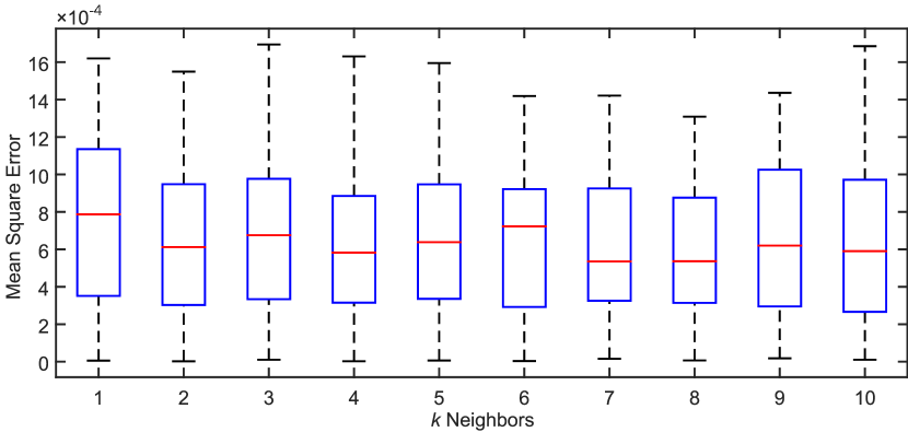
Figure 1: Imputation results for a crisp data-set

We notice that the best results occur for k=7, and k=8 with a mean square error (MSE) of $5.7$x$10^{-4}$ and the worst result for k=1 with a MSE of $7.9$x$10^{-4}$, which indicates a small deviation in the results showing that there is evidence that the algorithm is robust with regards to the chosen number of neighbours (k) considered during imputation.

4.1.2 Interval data-set

Next, we use interval data, consisting of measures of bats (made available by Billard et al. [1]) and the number of NaN ranging from 1 to 21, one obtains the box-plot in terms of mean square error shown in Figure 2.

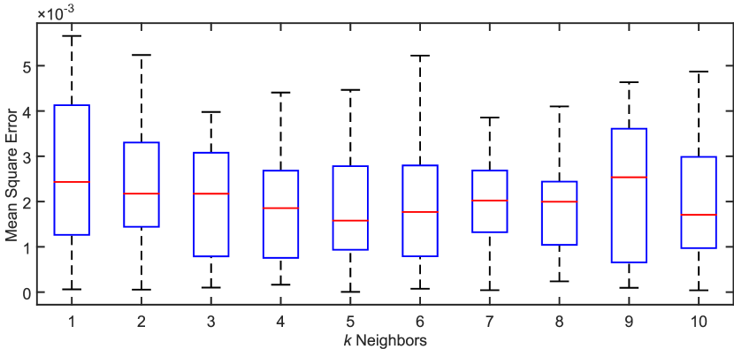
Figure 2: Imputation results for an interval data-set

We can observe that the best results occur for k=5 with a value of MSE of $1.6$x$10^{-3}$ and the worst result for k=9 with a value of MSE of $2.5$x$10^{-3}$. The results reveals that the algorithm is robust with regard to the number of neighbors considered.

4.1.3 Fuzzy data-set

Using fuzzy data, consisting of characteristics of Taiwanese teas (made available by Hung et al. [10]) and the number of NaNs ranging from 1 to 70, one obtains the results shown in the box-plot in Figure 3.

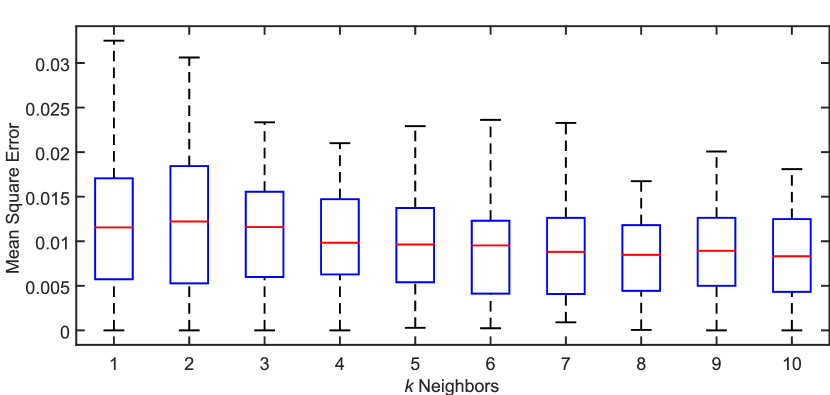
Figure 3: Imputation results for a fuzzy data-set

The box-plot shown in Figure 3 shows that the best results in terms of MSE occurs at k=10 with a value of $7.5$x$10^{-3}$ and the worst at k=2 with a value of $1.2$x$10^{-2}$. The algorithm kept the trend that points to robustness with regard to the amount of neighbors considered.

4.2 Heterogeneous Datasets

In this subsection we evaluate the algorithm with regard to heterogeneous datasets, especially small ones, where imputation becomes much harder.

4.2.1 Case Study 1

To better illustrate the algorithm, we run an iteration considering two nearest neighbors (k=2) for the data-set shown in Table 1, a decision making matrix made available by Fan et al. [5]. Let us refer to it as M.

0.5891	[0.31623, 0.94868]	[0.455842, 0.569803, 0.683763]
0.5624	[0.55470, 0.83205]	[0.371391, 0.557086, 0.742781]
0.5802	[0.55470, 0.83205]	[0.491539, 0.573462, 0.655386]

Table 1: Normalized decision matrix

Suppose the fuzzy data at $M_{3,3}$ is missing, as presented in Table 2.

0.5891	[0.31623, 0.94868]	[0.455842, 0.569803, 0.683763]
0.5624	[0.55470, 0.83205]	[0.371391, 0.557086, 0.742781]
0.5802	[0.55470, 0.83205]	NaN

Table 2: Decision matrix with missing value

Computing the distances using Eq. 8 one obtains a distance of 0.2661 to line 1 and 0.0945 to line 2. We can now compute the normalized weight using Eq. 7, which yields 0.2620 (line 1) and 0.7380 (line 2). Finally, we can impute the value according to Eq. 6 as $0.2620M_{1,3}+0.7380M_{2,3}$, resulting in $M_{3,3}=[0.3935,0.5604,0.7273]$, whose distance to the original value is of 0.0718 and a matrix mean square error of 0.0080.

Running the benchmark with the number of NaNs ranging from 1 to 3, one obtains the box-plot in terms of MSE shown in Figure 4.

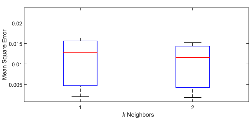
Figure 4: Imputation results for the matrix in Table 1

We can observe in Figure 4 promising results for imputation of heterogeneous data, with both instances having a MSE of about $1.2$x$10^{-2}$. These results are especially interesting given the size of the matrix and how fast it deteriorates with the increase of NaN. The results obtained by using the algorithm keeps the MSE in the same range as those shown in the case of homogeneous datasets.

4.2.2 Case Study 2

Applying the algorithm to a second benchmark involving a MCDM problem as presented in Table 3 by Jian-giang and Run-qi [12], one obtains the results in terms of MSE as shown in Figure 5.

0.47	[0.32, 0.48, 0.71]	[0.52, 0.67, 0.87]	[0.40, 0.55]
0.58	[0.16, 0.29, 0.47]	[0.26, 0.37, 0.52]	[0.41, 0.58]
0.42	[0.49, 0.67, 0.94]	[0.39, 0.52, 0.70]	[0.37, 0.54]
0.51	[0.32, 0.48, 0.71]	[0.26, 0.37, 0.52]	[0.50, 0.69]

Table 3: Multi-criteria decision making matrix

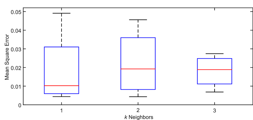
Figure 5: Imputation results for the matrix in Table 3

As expected, we notice in Figure 5 that the algorithm presents a better behavior in terms of MSE with a more sizable data-set, providing the best value of $1$x$10^{-2}$ for k=1, and the worst value of $1.9$x$10^{-2}$ for k=2.

4.2.3 Case Study 3

We consider now the MCDM matrix shown in Table 4 (Fan et al. [5]). The application of the algorithm provides the box-plot shown in Figure 6.

0.45	[0.60, 0.80]	[0.42, 0.57, 0.71]
0.41	[0.37, 0.93]	[0.27, 0.53, 0.80]
0.48	[0.32, 0.95]	[0.46, 0.57, 0.68]
0.43	[0.55, 0.83]	[0.37, 0.56, 0.74]
0.46	[0.20, 0.98]	[0.49, 0.57, 0.66]

Table 4: Multi-attribute decision matrix

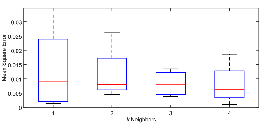
Figure 6: Imputation results for the matrix in Table 4

Using a data-set of about the same size as the one used in the previous case, but with more lines rather than columns (allowing more NaN and neighbours due to the benchmark mechanism, previously explained in Section 4), the algorithm provided similar results, as depicted in Figure 6. The best result in terms of MSE obtained was $5.1$x$10^{-3}$ for k=4 and the worst value of $5.8$x$10^{-3}$ for k=1.

5 Conclusions

Since the k-NN is a well established algorithm for classification, it has been extended to data imputation. Based on distance functions for the different data types used, the k-NN impute has been modified and good results in terms of MSE were obtained. First, the algorithm was tested for homogeneous data types, i.e., crisp, interval and fuzzy data. Next, in order to test the approach it was necessary to use datasets from clusterization and decision making since there are no widely known benchmarks for imputation with heterogeneous datasets. Imputation results for heterogeneous data in terms of MSE shows insensitivity with respect to the numbers of neighbors used.

For future studies we suggest the development of a way to find out the optimal number of neighbors in order to produce the best imputation results and also the expansion to other data types.

References

- Billard et al. [2008] Billard, L., Douzal-Chouakria, A., and Diday, E. (2008). Symbolic principal component for interval-valued observations.
- Brás and Menezes [2007] Brás, L. P. and Menezes, J. C. (2007). Improving cluster-based missing value estimation of dna microarray data. Biomolecular engineering, 24(2):273–282.
- Dasarathy [1991] Dasarathy, B. V. (1991). Nearest Neighbor (NN) Norms: NN Pattern Classification Techniques. IEEE Computer Society Press, Los Alamitos, CA.
- Derrac et al. [2014] Derrac, J., García, S., and Herrera, F. (2014). Fuzzy nearest neighbor algorithms: Taxonomy, experimental analysis and prospects. Information Sciences, 260:98 – 119.
- Fan et al. [2013] Fan, Z.-P., Xiao, Chen, F.-D., and Liu, Y. (2013). Extended TODIM method for hybrid multiple attribute decision making problems. Knowledge-Based Systems, 42:40 – 48.
- Fix and Hodges Jr [1951] Fix, E. and Hodges Jr, J. L. (1951). Discriminatory analysis-nonparametric discrimination: consistency properties. Technical report, DTIC Document.
- Folguera et al. [2015] Folguera, L., Zupan, J., Cicerone, D., and Magallanes, J. F. (2015). Self-organizing maps for imputation of missing data in incomplete data matrices. Chemometrics and Intelligent Laboratory Systems, 143:146 – 151.
- Garcia-Laencina et al. [2010] Garcia-Laencina, P. J., Sancho-Gomez, J.-L., and Figueiras-Vidal, A. R. (2010). Pattern classification with missing data: A review. Neural Computing and Applications, 19(2):263–282.
- Heitjan and Rubin [1991] Heitjan, D. F. and Rubin, D. B. (1991). Ignorability and coarse data. The Annals of Statistics, 19:2244–2253.
- Hung et al. [2010] Hung, W.-L., Yang, M.-S., and Lee, E. S. (2010). A robust clustering procedure for fuzzy data. Computers & Mathematics with Applications, 60(1):151 – 165.
- JCMB [2015] JCMB (2015). Download raw weather data. [Online; accessed 16-April-2015].
- Jian-giang and Run-qi [2008] Jian-giang, W. and Run-qi, W. (2008). Hybrid random multi-criteria decision-making approach with incomplete certain information. In Chinese Control and Decision Conference, 2008. CCDC 2008., pages 1444–1448.
- Jonsson and Wohlin [2004] Jonsson, P. and Wohlin, C. (2004). An evaluation of k-nearest neighbour imputation using likert data. In IEEE Procedings of 10th International Symposium on Software Metrics, 2004., pages 108–118.
- Little and Rubin [1986] Little, R. J. A. and Rubin, D. B. (1986). Statistical Analysis with Missing Data. John Wiley & Sons, Inc., New York, NY, USA.
- Lourenzutti and Krohling [2015] Lourenzutti, R. and Krohling, R. A. (2015). TODIM based method to process heterogeneous information. Procedia Computer Science, 55:318 – 327.
- Ma et al. [2009] Ma, J., , G., Lu, J., and Ruan, D. (2009). Impute missing assessments by opinion clustering in multi-criteria group decision making problems. In Carvalho, J. P., Dubois, D., Kaymak, U., and da Costa Sousa, J. M., editors, IFSA/EUSFLAT Conf., pages 555–560.
- Rana et al. [2012] Rana, S., John, A., and Midi, H. (2012). Robust regression imputation for analyzing missing data. In International Conference on Statistics in Science, Business, and Engineering (ICSSBE), 2012, pages 1–4.
- Silva-Ramírez et al. [2015] Silva-Ramírez, E.-L., Pino-Mejías, R., and López-Coello, M. (2015). Single imputation with multilayer perceptron and multiple imputation combining multilayer perceptron and k-nearest neighbours for monotone patterns. Applied Soft Computing, 29:65 – 74.
- Troyanskaya et al. [2001] Troyanskaya, O. G., Cantor, M. N., Sherlock, G., Brown, P. O., Hastie, T., Tibshirani, R., Botstein, D., and Altman, R. B. (2001). Missing value estimation methods for DNA microarrays. Bioinformatics, 17(6):520–525.