Contexts and Data Quality Assessment

Abstract

The quality of data is context dependent. Starting from this intuition and experience, we propose and develop a conceptual framework that captures in formal terms the notion of context-dependent data quality. We start by proposing a generic and abstract notion of context, and also of its uses, in general and in data management in particular. On this basis, we investigate data quality assessment and quality query answering as context-dependent activities. A context for the assessment of a database $D$ at hand is modeled as an external database schema, with possibly materialized or virtual data, and connections to external data sources. The database $D$ is put in context via mappings to the contextual schema, which produces a collection $\mathcal{C}$ of alternative clean versions of $D$. The quality of $D$ is measured in terms of its distance to $\mathcal{C}$. The class $\mathcal{C}$ is also used to define and do quality query answering. The proposed model allows for natural extensions, like the use of data quality predicates, the optimization of the access by the context to external data sources, and also the representation of contexts by means of more expressive ontologies.

Keywords:  Data quality, data cleaning, contexts, schema mappings, virtual data integration, query answering.

1 Introduction

The assessment of the quality of a data source is context dependent, i.e. the notions of “good” or “poor” data cannot be separated from the context in which the data is produced and used. For instance, the data about yearly sales of a product with seasonal variations might be considered quality data by a business analyst assessing the yearly revenue of a product. However, the same data may not be good enough for a warehouse manager who is trying to estimate the orders for next month.

In addition, data quality is related to the discrepancy between the actual stored values and the “real” values that were supposed to be stored. For instance, if a temperature measurement is taken with a faulty thermometer, the stored value (the measurement) would differ from the right value (the actual temperature), which was the one supposed to be stored. This is an example of semantically inaccurate data [7].

Another type of semantic discrepancy occurs when senses or meanings attributed by the different agents to the actual values in the database disagree [46], as shown in the Example 1. In this paper, we focus on data quality (DQ) problems caused by this type of semantic discrepancy.

Example 1

Tom is a patient in a hospital. Several times a day his temperature is measured and recorded by a nurse. His doctor, John, wants to see Tom’s temperature around noon every day to follow his evolution. The information that John needs appears in the TempNoon relation of Table 2, which contains the temperatures between 11:30 and 12:30 per day for each of John’s patients.

	TempNoon
	Patient	Value	Time	Date
1	Tom Waits	38.5	11:45	Sep/5
2	Tom Waits	38.2	12:10	Sep/5
3	Tom Waits	38.1	11:50	Sep/6
4	Tom Waits	38.0	12:15	Sep/6
5	Tom Waits	37.9	12:15	Sep/7

Table 1:

	TempNoon​’
	Patient	Value	Time	Date
1	Tom Waits	38.5	11:45	Sep/5
2	Tom Waits	38.0	12:15	Sep/6
3	Tom Waits	37.9	12:15	Sep/7

Table 2:

John has additional quality requirements for the temperature measurements of his patients: they have to be taken by a certified nurse with an oral thermometer. On Sep/5, unaware of the new requirements, Cathy takes Tom’s temperature at 12:10 with a tympanal thermometer and records the result as the tuple number 2 in Table 2. Since the instrument used does not appear in the table, John interprets the 38.2^oC value as taken with an oral thermometer.

This is an example of a discrepancy between the semantics of the value as intended by the data producer (38.2^oC taken with a tympanal thermometer) and the semantics expected by the data consumer (38.2^oC taken with an oral thermometer). This tuple should not appear in a quality table, i.e. one that satisfies John’s quality requirements, since such a table would contain only temperatures taken with an oral thermometer.

A similar problem appears in the third tuple in Table 2: it was taken by a new nurse, Helen, who is not yet certified, and thus, does not satisfy one of the doctor’s requirements. This tuple should not appear in a quality table containing only temperatures taken by certified nurses.

Table 2 fixes the problems of Table 2 with respect to the doctor’s specification: the problematic second and third tuples do not appear in it.

How can we say or believe that Table 2 does contain only quality data? Prima facie it does not look much different from Table 2. This positive assessment would be possible if we had a contextual database containing additional information, e.g. Tables 4, 4 and 5.

	S (shift)
	Date	Shift	Nurse
1	Sep/5	morning	Susan
2	Sep/5	afternoon	Cathy
3	Sep/5	night	Joan
4	Sep/6	morning	Helen
5	Sep/6	afternoon	Cathy
6	Sep/6	night	Cathy
7	Sep/7	morning	Susan
8	Sep/7	afternoon	Susan
9	Sep/7	night	Joan

Table 3:

	C (certification)
	Name	Year
1	Ann	2003
2	Cathy	2009
3	Irene	2000
4	Karen	1995
5	Nancy	1995
6	Natasha	2001
7	Susan	1996

Table 4:

	I (instrument)
	Nurse	Date	Instr	Type
1	Susan	Sep/5	Therm.	Oral
2	Susan	Sep/5	BPM	Arm
3	Cathy	Sep/5	Therm.	Tymp
4	Cathy	Sep/5	BPM	Arm
5	Joan	Sep/5	Therm.	Tymp
6	Helen	Sep/6	Therm.	Oral
7	Cathy	Sep/6	Therm.	Oral
8	Cathy	Sep/6	BPM	Arm
9	Susan	Sep/7	Therm.	Oral
10	Joan	Sep/7	Therm.	Oral

Table 5:

Table 4 contains the name of the nurses in Tom Waits’ ward and the shifts they work in by day. These are the nurses taking the measurements; since it is a small ward there is only one nurse per shift with that task. Table 4 records the names of the certified nurses in the ward and the year they got the certification. Table 5 contains the type of instrument each nurse is using by day (e.g., thermometer, blood pressure monitor (BPM)), and its type (e.g., arm or wrist for BPM, and oral or tympanal for thermometer). Each nurse takes all temperature measurements of the day using the same type of instrument. This contextual information allows us to assess the quality of the data in Tables 2 and 2. $\blacksquare$

This paper captures and formalizes the intuition and experience that data quality is context dependent. This requires an appropriate formalization of context. In our case, this is given as a system of integrated data and metadata of which the data source under quality assessment can be seen as a particular and special component.

More precisely, the context for the assessment of a certain instance $D$ of schema $\mathcal{S}$ with respect to data quality is given by an instance $I$ of a possibly different schema $\mathcal{C}$, which could be an extension of $\mathcal{S}$. In other words, $D$ could be seen as a “footprint” of a the contextual, extended database $I$.

In order to assess the quality of $D$, it has to be “put in context”, which is achieved by mapping $D$ (and $\mathcal{S}$) into the contextual schema and data; the extra information in $I$ is what gives context to, and explains, the data in $D$. Actually, $\mathcal{C}$ can be more complex than a single schema or instance, namely a collection of database schemas and instances interrelated by data- and schema mappings.

The contextual schema and data are not necessarily used to enforce quality of a given instance. Instead, it can be used to: (a) Assess the quality of the data in the instance at hand; (b) Characterize the quality answers to queries; and (c) Possibly obtain those quality answers to a user query.

Instance $I$ above could be replaced by a much richer contextual description, e.g. a full-fledged ontology. Along this line, but still in a classic database scenario, we might define some additional data quality predicates on top of $\mathcal{C}$ [46]. They could be used to assess the quality of the data in $D$, and also the quality of query answers from $D$, as we will explore later.

The following contributions can be found in this paper:

• We propose a general model of context and describe how it can be used for data quality assessment.

• We apply the context model to:

  • Quality (or clean) query answering, i.e. for characterizing and possibly computing quality query answers. We concentrate on monotone queries.

  • Data quality assessment via some natural data quality measures that emerge directly from the model.

• We propose algorithms for the previously mentioned tasks for a few particular, but common, cases. For example, when we have a contextual instance $I$ that can be used for quality assessment. We also present an algorithm for quality query answering under this assumption. Another special case we consider is when such a contextual instance does not exist. It has to be first (re)created from the available information and the metadata.

• We indicate how our general framework could be naturally extended in subsequent work to include other features, like externally defined quality predicates

• In addition, we propose a general notion of context, not only for data quality purposes. In the light of this general model, we discuss other tasks that can be undertaken on the basis of contexts. The contexts used in data quality are then shown to be a special case of this general and abstract framework.

The rest of the paper is organized as follows. In Section 2 we introduce a few basic notions of data management. In Section 3 we introduce our general, abstract notion of context, and we show how it can be applied in data management in general. In Section 4, we present a general framework for contextual data quality assessment, introducing intended quality instances and quality query answers. In Sections 5 and 6, we consider in more detail two special cases of the general framework. In Section 7 we propose some measures for data quality assessment in the presence of multiple quality instances. We discuss related work in Section 8. We draw final conclusions and point out to ongoing and future work in Section 9. This paper builds on [12], and extends it in several ways. In the Appendix we develop some ideas on contexts that access external sources.

2 Preliminaries

We will consider relational schemas, say $\mathcal{S}$, with database predicates $R,\ldots\in\mathcal{S}$, and an underlying data domain $\mathcal{U}$. A schema determines a language $L(\mathcal{S})$ of first-order predicate logic. Queries and views are defined by formulas of $L(\mathcal{S})$. In this paper we consider only conjunctive queries and views, i.e. with definitions of the form

$$\mathcal{Q}(\bar{x})\!:\ \exists\bar{y}(A_{1}(\bar{x}_{1})\wedge\cdots\wedge A_{n}(\bar{x}_{n})),$$ (1)

where the $A_{i}(\bar{x}_{i})$ are atoms with database or built-in predicates. Here, $\bar{x}$ contains the free variables of the query (or view), i.e. that appear in some $\bar{x}_{i}$, but not in $\bar{y}$. The atoms may contain domain constants (i.e. element of $\mathcal{U}$). Then, these queries and views are monotone. Conjunctive queries and unions thereof can be expressed in non-recursive Datalog with built-ins [1, 28]; i.e by a finite set of rules of the form:

$${\it Ans}_{\mathcal{Q}}(\bar{x})\leftarrow R_{1}(\bar{x}_{1}),\ldots,R_{n}(\bar{x}_{n}),\varphi,$$ (2)

where $R_{i}\in\mathcal{S}$, $\bar{x},\bar{x}_{i}$ are tuples of variables with $\bar{x}\subseteq\cup_{i}\bar{x}_{i}$, and $\varphi$ is a conjunction of built-in atoms. ${\it Ans}_{\mathcal{Q}}$ is a new predicate whose extension collects the query answers. Sometimes, we will identify the query with the answer predicate, simply writing $\mathcal{Q}(\bar{x})\leftarrow R_{1}(\bar{x}_{1}),\ldots,R_{n}(\bar{x}_{n}),\varphi$.

An instance $D$ for schema $\mathcal{S}$ is a finite set of ground atoms (no variables). If $R\in\mathcal{S}$ is a database predicate, $R(D)$ denotes its extension in $D$. That is, for each database predicate $R\in\mathcal{S}$, $R(D)\subseteq D$. Instances $D,R(D),\ldots$ are those that will be under quality assessment with respect to to a contextual system. Similarly, $\mathcal{Q}(D)$ denotes the set of answers to query $\mathcal{Q}$ from instance $D$, and $V(D)$ denotes the extension of the view $V$ on $D$.

For a given schema, say $\mathcal{S}$, integrity constraints (ICs) are sentences written in $L(\mathcal{S})$. An instance for $\mathcal{S}$ is consistent when $D$ satisfies a given set $\Sigma$ of ICs, denoted $D\models\Sigma$. For more basic concepts of relational databases see [1].

We will assume basics concepts related to schema mappings, as those found in virtual data integration systems (VDISs) [50, 10], data exchange [48, 4], or in peer data management systems [15]. (See [29] for connections between these three areas.) In general terms, schema mappings take the form of correspondences between two formulas, like queries or view definitions, each of them containing predicates from a single or several schemas. In particular, a data source under assessment $D$ may have a schema that is mapped into a contextual schema.

We assume that the reader knows the basic concepts of virtual data integration systems, in particular, the notions of open (or sound) source, closed (or complete) source, and exact (or clopen) source [50, 10, 41]. For summary and reference, we list below some common forms of associations, or mappings:

• $\forall\bar{x}(S(\bar{x})\rightarrow\varphi_{{}_{\mathcal{G}}}(\bar{x}))$, where $S$ is a relational predicate of a data source and $\varphi_{{}_{\mathcal{G}}}(\bar{x})$ is a conjunctive query over a global relational schema $\mathcal{G}$. These association can be found in VDISs under the local-as-view (LAV) paradigm with open (or sound) sources.

• $\forall\bar{x}(\psi_{{}_{\mathcal{S}}}(\bar{x})\rightarrow G(\bar{x}))$, as found in global-as-view (GAV) VDISs with open sources, where $\psi_{{}_{\mathcal{S}}}(\bar{x})$ is a conjunctive query over the union $\mathcal{S}$ of relational source schemas, and $G$ is a global relational predicate.

• $\forall\bar{x}(\psi_{{}_{\mathcal{S}}}(\bar{x})\rightarrow\varphi_{{}_{\mathcal{G}}}(\bar{x}))$, as in global-and-local-as-view (GLAV) VDISs with open sources. They are associations between views (or queries) over the source schemas and a global schema, resp.

We can see these schema mappings as metadata, i.e. data about data; in this case describing data associations. This second layer of data can be stored and computationally processed [3, 9]. Other examples of metadata are relational schemas, integrity constraints (ICs), view definitions, access and privacy restrictions, trust, and also quality constraints [33].

3 On Contexts and their Uses

As we have stressed above, a full assessment of the quality of data cannot be conducted in isolation; it only makes sense in a broader setting. Quality depends, among other things, on the context that allows us to make sense of the data and assess it. As expected, the notion of context is not only related to data quality, but to many other activities, within and outside computer science.

In computer science we find the term “context” in several places , e.g. databases, semantic web, knowledge representation, mobile applications, etc. It is usually used under context awareness [5], e.g. context-aware search, context-aware databases (and query answering), context-aware mobile devices [36], etc. . However, most of the time there is no explicit notion of context, but only some algorithms that take into account (or into computation) some obvious contextual aspects. Most typically, time and geographic location, i.e. particular dimensions, and not much beyond.

This makes it clear that there is a lack of research around the notion of context, at least as used in computer science and engineering. A precise and formalized general notion of context becomes necessary. This applies in particular to the use of contexts -and metadata in general- for data quality assessment and data cleaning.

It is important to emphasize that, as with contexts in computer science, there hasn’t been much scientific or fundamental research in the area of data quality and data cleaning. In general, research in this area tends to be rather ad hoc, where vertical, non-extendable, non-adaptable solutions (usually of an algorithmic nature) are provided for specific problems and in specific domains. We are not aware of the existence of an all-encompassing, general logical theory of contexts, even less for those that appear in data management. Only some aspects of them have been used and formalized.

In this work we make an attempt to contribute with some fundamental research around certain aspects of general contexts, or better, a general theory of context that can be applied, in particular, to data management; and even more specifically, to data quality. After all, it is clear that the meaning, usability and quality of data, among other features of data, largely depend on the context in which data is placed or handled.

Our general perception and formalization of contexts is inspired by their use in data quality assessment and cleaning. We see contexts as a form of metadata that can be formalized as a semantic layer and represented as an ontology, or more generally, as a theory. With this intuitions, we now describe some of the elements that we envision in such a general notion of context.

First of all, what is “put in context” is a logical theory, say $\mathcal{T}$. The actual context is another separate logical theory, say $\mathfrak{C}$. These two theories are expressed in corresponding logical languages with their logical semantics. Theories $\mathcal{T}$ and $\mathfrak{C}$ may share some predicate symbols. The connection between $\mathcal{T}$ and $\mathfrak{C}$ is established through predicates and logical mappings, i.e. logical formulas (cf. Figure 1). For example, we could have mappings of the kind found in virtual data integration or data exchange (cf. Section 2); or in mathematical logic under “interpretation between theories” [32, sec. 2.7], a notion that allows us sometimes to embed a theory into another.

In principle, theories $\mathcal{T}$ and $\mathfrak{C}$ can be written in any formal logic, not necessarily classical predicate logic, and the same applies to the mappings.

Figure 1: General Contexts

Several uses of, and tasks associated to, contexts naturally come to our mind; among them:

• Capturing and narrowing down semantics at $\mathcal{T}$’s level. This can be achieved by defining in $\mathfrak{C}$ predicates that are used in $\mathcal{T}$, e.g. “time close to noon” in our running example. Context $\mathfrak{C}$ can also contribute with additional semantic constraints on predicates used in $\mathcal{T}$, e.g. ICs on table TempNoon in the example. In particular, quality constraints [33, 14] could be used as semantic constraints at this level.

• Providing on the basis of $\mathfrak{C}$, a notion and representation of the sense of terms in $\mathcal{T}$. Sense is intuitively associated to context, and it has been a subject of preliminary investigation in data quality [46]. Moreover, the study of sense vs. denotation (or reference) has been a subject of logical investigation at least since Frege’s work [35]. The notion of sense should be revisited in a contextual framework. A context should also support disambiguation of terms appearing in $\mathcal{T}$. This is also related to meaning or semantics, and a typical contextual task.

• Providing for dimensions and points of view, to be used for analysis and understanding of $\mathcal{T}$’s knowledge. A general definition and formalization of dimension based on contexts is worth exploring. In particular, to be applied to problems of data quality, as view points for quality assessment.

• Specifying and using notions of relevance for theory $\mathcal{T}$.

• Providing the conceptual basis and tools for explanation, diagnosis, and analysis of causality [56].

• Capturing through context $\mathfrak{C}$ common sense assumptions and practices to be applied to $\mathcal{T}$.

• Different forms of assessment of $\mathcal{T}$, e.g. data quality.

This is only of partial list of intuitions, notions, and tasks that we usually associate to the concept of context. Each of them, and others, could give rise to a full and long term research program. Some of the open research directions are related to the identification of representation formalisms, and also computational processing mechanisms for/of contextual information, in combination with the theory (or data) it is contextualizing.

It is important to realize that our context-dependent data quality assessment problem becomes a particular case of our general concept of context. In the rest of this section, we briefly provide support for this claim, by indicating how the elements of the contextual framework in Figure 1 would appear in the case of data quality assessment. In the following section we provide specific details.

3.1 Databases and the general contextual framework

In this section we show in general terms that our abstract model of context can be applied to data management in general. It may not be obvious that relational databases, for example, can be seen as theories; and that other data management system, like mediators for virtual data integration, can also be seen as theories.

In Figure 1, the theory $\mathcal{T}$ could be a relational database instance $D$ for a relational schema $\mathcal{S}$, with $D$ under quality assessment. Instance $D$ can be represented as a theory written in first-order predicate logic (FOPL) by appealing to Reiter’s logical reconstruction of a relational database [61]. It allows to transform the database $D$, usually conceived and treated as a model-theoretic structure, into a logical theory, $\mathcal{T}(D)$.

According to Reiter’s reconstruction, query answering from $D$, in particular, becomes expressed as logical entailment and reasoning from $\mathcal{T}(D)$. Similarly, IC satisfaction becomes logical entailment (of the IC) [62].

For example, relation TempNoon in Example 1 (Table 2) can be reconstructed by means of axiom (3.1) below plus unique names and, possibly, domain closure axioms [61].

$$\forall wxyz(\textbf{TempNoon}(w,x,y,z) ~{}\equiv~{} ((w=\mbox{Tom Waits}\wedge\cdots\wedge z=\mbox{Sep/5})$$

$$~{}~{}~{}~{}~{}~{}~{}~{}~{}~{}~{}~{}\vee\ \cdots\ \vee$$

$$(w=\mbox{Tom Waits}\wedge\cdots\wedge z=\mbox{Sep/7}))).$$

Instance $D$ (think of TempNoon) has to be “put in context”, i.e. it has to be mapped into context $\mathfrak{C}$.

Now, $\mathfrak{C}$ could be given as a contextual schema $\mathcal{C}$, plus a possibly incomplete instance $C$ for $\mathcal{C}$, and a set of quality predicates $\mathcal{P}$ with definitions in $\mathfrak{C}$. That is, a context would be, in turn, something like a a virtual or (semi)materialized data integration system (DIS).

If the contextual data is incomplete, there will be only a partial specifications of predicates in FOPL. For example, if the contextual relation S in Table 4 is displaying only incomplete data, we will have, in contrast with axiom (3.1) that uses a double implication, an axiom with a unidirectional implication:

$$\forall xyz(\textbf{S}(x,y,z) ~{}\leftarrow~{} ((x=\mbox{Sep/5}\wedge\cdots\wedge z=\mbox{Susan})\ \vee\cdots\ \vee$$

$$~{}~{}~{}~{}~{}~{}~{}~{}~{}~{}~{}~{}~{}~{}~{}~{}~{}~{}~{}~{}~{}~{}~{}(x=\mbox{Sep/7}\wedge\cdots\wedge z=\mbox{Joan}))).$$

In addition, there will be logical mappings between $D$ and $\mathfrak{C}$, like those of the forms 1.-3. at the end of Section 2. We could also have ICs and view definitions in $\mathfrak{C}$. This is all metadata that can also be expressed as a part of a logical theory.

To make this more concrete, we could introduce at $\mathfrak{C}$’s level a “nickname”, $\textbf{TN}_{\mathcal{C}}$ for relation TempNoon in $D$, and have the mapping

$$\forall\bar{x}(\textbf{TempNoon}(\bar{x})\rightarrow\textbf{TN}_{\mathcal{C}}(\bar{x}))$$ (5)

that maps TempNoon into $\textbf{TN}_{\mathcal{C}}$. The latter could be further combined with $\mathfrak{C}$’s data, to provide the desired information about the nurse certification status of nurse taking temperature, through a view (we use Datalog notation for its definition):

$${\it CertTemp}(m,t,d) ~{}\leftarrow~{} \textbf{TN}_{\mathcal{C}}(\text{Tom Waits},m,t,d),\ \textbf{S}(d,s,n),$$

$$\hskip 93.89418pt\textbf{C}(n,y),\ {\it Times}(t,s).$$

This view collects the temperature measurements ($m$), with their dates ($d$) and times $(t$), that were taken by certified nurses. Relation ${\it Times}$ is used to check if a particular time $t$ falls within a shift $s$. The view extension can be used for further analysis of $D$’s data.

We could also replace the view defined in (3.1) by a more general one, e.g.

$$\textbf{TempNoon}^{\it Cf}(p,m,t,d) ~{}\leftarrow~{} \textbf{TN}_{\mathcal{C}}(p,m,t,d),\ \textbf{S}(d,s,n),$$

$$\hskip 93.89418pt\textbf{C}(n,y),\ {\it Times}(t,s),$$

that now collects the patient names, possibly other than Tom. The new view predicate, $\textbf{TempNoon}^{\it Cf}$, does not belong to the schema containing the original predicate TempNoon. However, it could be seen as a new version of the latter that now takes into account the certification of nurses as a particular quality concern.

We can see that the use of a relational ontology, providing a context for a relational instance $D$, becomes a particular case of the general framework illustrated in Figure 1. In the following sections we will present more specific details and concrete examples.

4 Contexts for Data Quality Assessment

4.1 The general approach

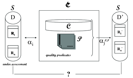
Figure 2: Data Quality Context

We start by describing in general terms our approach to context-based data quality assessment and context-based quality query answering. Figure 2 illustrates the main high-level ideas.

Assume we have a database instance $D$ for schema $\mathcal{S}$; and we want to assess $D$’s data quality. $D$ is then put into context $\mathfrak{C}$ via some mappings (the $\alpha_{i}$ in the figure). The data in $D$’s image in $\mathfrak{C}$ are combined with additional information existing in, or available from, $\mathfrak{C}$. This additional information can be local data at $\mathfrak{C}$, definitions of quality predicates, additional semantic constraints, and even data from external sources (cf. the Appendix).

The combination at $\mathfrak{C}$ of $D$’s original data with the contextual information produces (via the mappings $\alpha_{j}$ on the RHS of the figure) a new version $D^{\prime}$ of $D$, or possible a class $\mathcal{D}$ of several new, admissible versions of $D$, where the quality concerns are captured or enforced. This process is also illustrated in Figure 3.

The idea behind context-based data quality assessment is that $D^{\prime}$ has the correct, clean contents that $D$ should have (e.g. Table 2 for TempNoon in Example 1). And $D$ can be compared with $D^{\prime}$. For example, the extension for the view in (3.1) can be compared with the subrelation of TempNoon in $D$ that contains the entries for Tom, at least with respect to to the certification status. Similarly, the entire relation TempNoon could be compared with the relation $\textbf{TempNoon}^{\it Cf}$ defined in (3.1).

As just suggested, the quality of instance $D$ can be measured by comparing it with the resulting instance $D^{\prime}$ (or collection $\mathcal{D}$ thereof). And quality answers to queries posed to original instance $D$ can be defined and computed as answers to the same query that are true of $D^{\prime}$, or of all the admissible $D$’ if there are several of them. As we will see below, quality assessment and quality query answering are closely related.

The mappings between $D$ (or rather its schema $\mathcal{S}$) and $\mathfrak{C}$ can take different forms. In this paper, we will appeal to a common practice in virtual data integration systems of introducing nicknames in $\mathfrak{C}$ for the predicates in $\mathcal{S}$. This is not strictly necessary, but simplifies the presentation, without losing generality. If an original predicate $R\in\mathcal{S}$ has a more elaborate mapping with predicates in in $\mathfrak{C}$, we capture this association as one involving $R^{\prime}$, the nickname predicate for $R$.

4.2 The contextual framework

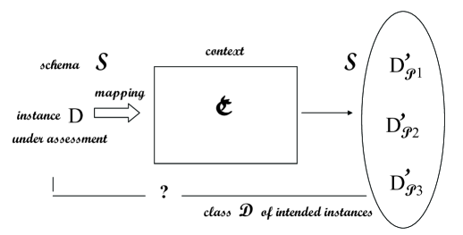
Figure 3: Using a Context for Quality Assessment

We have a relational schema $\mathcal{S}=\{R_{1},\ldots,R_{n}\}$, and also a contextual relational schema $\mathcal{C}$ (including built-ins). The participating schemas are related by schema mappings. In particular, the data source under assessment $D$ may be mapped into the contextual schema.

A common form of mapping is of the form

$$\alpha_{{}_{R}}\!:\ \ \forall\bar{x}(R(\bar{x})\ \rightarrow\ \varphi^{\mathcal{C}}(\bar{x})),$$ (8)

where $R\in\mathcal{S}$, $\varphi^{\mathcal{C}}(\bar{x})$ is a conjunctive query over schema $\mathcal{C}$.

We may assume that $\mathcal{C}$ has a subschema $\mathcal{S}^{\prime}$ that is a copy of $\mathcal{S}$ formed by nicknames $R^{\prime}$ of predicates $R$ in $\mathcal{S}$. In this case, we may have simple copying mapping of the form

$$\alpha_{{}_{R}}\!:\ \ \forall\bar{x}(R(\bar{x})\ \rightarrow\ R^{\prime}(\bar{x})),$$ (9)

as in (5). We could further apply the the closed-world assumption (CWA) [61] to $R^{\prime}$, obtaining  $\alpha_{{}_{R}}\!:\ \forall\bar{x}(R(\bar{x})\ \equiv\ R^{\prime}(\bar{x})$.

We also have an instance $D$ for $\mathcal{S}$. The extensions of predicates $R\in\mathcal{S}$ in $D$ are denoted with $R(D)$. By applying the mappings $\alpha_{i}$ to $D$, we obtain (possibly virtual) extensions $R^{\prime}(D)$ inside $\mathfrak{C}$ for the nickname predicates $R^{\prime}$. We obtain an instance

$$D^{\prime}\ :=\ \bigcup_{R\in\mathcal{S}}R^{\prime}(D),$$ (10)

at the contextual level, for schema $\mathcal{S}^{\prime}$.

In addition to the contextual schema $\mathcal{C}$ we may have a set $\mathcal{P}$ of contextual quality predicates (CQPs) with definitions inside $\mathfrak{C}$. In principle they could be defined entirely in terms of (or as views over) schema $\mathcal{C}$. However, we keep them separate to emphasize their role in capturing data quality concerns. We obtain a combined contextual schema $\mathcal{C}\cup\mathcal{P}$. Typically, each $P\in\mathcal{P}$ is defined as a conjunctive view

$$P(\bar{x})\ \leftarrow\ \gamma^{\mathcal{C}}(\bar{x}),$$ (11)

in terms of elements of $\mathcal{C}$ (and possibly built-in predicates).

The relations $R^{\prime}(D)$ inside $\mathfrak{C}$ can be further processed by applying new mappings $\alpha_{j}^{\mathcal{C,P}}$. Their application logically combine the $R^{\prime}(D)$s with additional information captured via the schema (and possibly data for) $\mathcal{C}\cup\mathcal{P}$ at $\mathfrak{C}$.

Actually, the ideal, quality extension of predicate $R\in\mathcal{S}$ is obtained as the extension of a new predicate (or view) $R^{\prime}_{\mathcal{P}}$. It is obtained by applying a mapping $\alpha_{{}_{R}}^{\mathcal{C,P}}$ to $D^{\prime}$ as in (10) (possibly only $R^{\prime}(D)$) and also additional contextual data and metadata, including CQPs in $\mathcal{P}$. The mappings or view definitions are as follows:

$$\alpha_{{}_{R}}^{\mathcal{C,P}}\!:\ \ \forall\bar{x}(\psi^{\mathcal{C,P}}\!(\bar{x})\ \rightarrow\ R^{\prime}_{\mathcal{P}}(\bar{x})),$$ (12)

where $\psi^{\mathcal{C,P}}$ is a conjunctive query over schema $\mathcal{C}\cup\mathcal{P}$. Notice that $\mathcal{C}$ contains schema $\mathcal{S^{\prime}}$. An example of this kind of definition is (3.1).

A special and common case corresponds to definitions via conjunctive views of the form:

$$\alpha_{{}_{R}}^{\mathcal{C,P}}\!:\ \ R^{\prime}_{\mathcal{P}}(\bar{x})\ \longleftarrow\ \varphi_{{}_{R}}^{\mathcal{C}}(\bar{x}_{1}),\ \varphi_{{}_{R}}^{\mathcal{P}}(\bar{x}_{2}),$$ (13)

where $\bar{x}\subseteq\bar{x}_{1}\cup\bar{x}_{2}$, and $\varphi_{{}_{R}}^{\mathcal{C}}(\bar{x}_{1}),\varphi_{{}_{R}}^{\mathcal{P}}(\bar{x}_{2})$ are in their turn conjunctions of atomic formulas with predicates in $\mathcal{C}$, $\mathcal{P}$, respectively. A particular case is obtained when in (13) there are no CQPs, i.e.

$$R^{\prime}_{\mathcal{P}}(\bar{x})\ \longleftarrow\ \psi_{{}_{R}}^{\mathcal{C}}(\bar{x}_{1}).\vspace{-3mm}$$ (14)

However, we still keep the subscript $\mathcal{P}$ to establish the difference with $R^{\prime}$. Each predicate $R^{\prime}_{\mathcal{P}}$ can be seen as a quality nickname for predicate $R\in\mathcal{S}$.

Intuitively, CQPs can be used to express an atomic quality requirement requested by a data consumer or met by a data producer. With them we can restrict the admissible values for certain attributes in tuples, so that only quality tuples find their way into a quality version of the database.

Although CQPs can be eliminated by unfolding their Datalog definitions (11), we make them explicit here, for several reasons:

• First, as mentioned above, to emphasize their role as predicates capturing quality requirements.

• They allow us to compare data quality requirements in a more concrete way.  For example, it is obvious that the quality requirement “temperature values need to be measured by an oral or tympanal thermometer” is less restrictive than “temperature values need to be measured by an oral thermometer”.

• Our approach allows for the consideration of CQPs that are not defined only in terms of $\mathcal{C}$ alone, but also in terms of other external sources, that is, by view definitions of the form $P(\bar{x})\leftarrow\gamma^{\mathcal{C}}(\bar{x}),\gamma^{\mathcal{E}}(\bar{x})$, where $\gamma^{\mathcal{E}}$ is a formula expressed in terms of atoms that can be evaluated at/by external sources.

Several different assumptions can be made at this stage, e.g. about the kind of mappings involved ($\alpha$ or $\alpha^{\mathcal{C},\mathcal{P}}$), assumptions about them and their sources of data (e.g. openness, closeness, …), availability or not of an initial contextual instance and assumptions about it (e.g. (in)completeness), etc. Some special cases will be considered in Sections 5 and 6. The case of external sources in considered in the Appendix.

Actually, each of the mappings in Figure 2 could be view definitions (or view associations) of any of the LAV, GAV, GLAV forms described in Section 2, with additional assumptions about openness/closedness of the participating data sources.

More precisely, the different data sources, including the original $D$ and any at the context level, the definitions of the quality predicates in terms of elements in $\mathcal{C}$, the schema mappings and view definitions, etc., determine a collection $\mathcal{I}$ of admissible contextual instances (ACIs) for the contextual schema $\mathcal{C}$, as it is the case in virtual data integration and peer data exchange systems. Notice that each ACI $I\in\mathcal{I}$ may also depend on the original instance $D$ if the latter was mapped into the context.

4.3 Measuring data quality and quality answers

For a given ACI $I\in\mathcal{I}$, by applying the mappings (12), we obtain (possibly virtual) extensions $R^{\prime}_{\mathcal{P}}(I)$ for the predicates $R\in\mathcal{S}$. Notice that the collections of predicate extensions $R^{\prime}_{\mathcal{P}}(I)$s can be seen as a quality instance $D^{\prime}_{\mathcal{P}}(I)$ for the original schema $\mathcal{S}$.

As a consequence, we can assess the quality of $R(D)$ in instance $D$ through its “distance” to $R^{\prime}_{\mathcal{P}}(I)$; and the quality of $D$ in terms of an aggregated distance to $D^{\prime}_{\mathcal{P}}(I)$.

Different notions of distance might be used at this point. Just to fix ideas, we can think of using, e.g. the numerical distance $|R(D)\bigtriangleup R^{\prime}_{\mathcal{P}}(I)|$ of the symmetric difference between the two $R$-instances. And for the whole instance, e.g. the quality measure:

$${\it qm}_{\!0}(D)\ :=\ \sum_{R\in\mathcal{S}}|R(D)\bigtriangleup R^{\prime}_{\mathcal{P}}(I)|.$$ (15)

Since we can have several contextual instances $I\in\mathcal{I}$, we can have a whole class $\mathcal{D}$ of instances $D^{\prime}_{\mathcal{P}}(I)$, with $I\in\mathcal{I}$. (Actually, we could have none if contextual ICs are imposed, i.e. at $\mathfrak{C}$’s level.)

This situation is illustrated in Figure 3. In the case of multiple “intended” clean instances, related to a whole class $\mathcal{I}$ of ACIs, $D$ would have to be compared with a whole class of quality instances

$$\mathcal{D}:=\{D^{\prime}_{\mathcal{P}}(I)~{}|~{}I\in\mathcal{I}\};$$ (16)

and more elaborate measures of distance can be used. We present them in Section 7, after developing a scenario, in Section 6, where those multiple instances naturally appear.

At this point we can introduce the notion of quality query answering about (or from) $D$. The idea is to retrieve clean answers from the original instance $D$. Since the latter may be dirty, direct, classic query answering from $D$ is not intended. Instead, clean answers can be obtained from $D^{\prime}_{\mathcal{P}}(I)$ (or the collection of them).

Example 2

(example 1 continued) Consider a query about patients and their temperatures around noon on Sep/5:

$$\mathcal{Q}(p,v)\!:\ \exists t\exists d({\it\textbf{TempNoon}}(p,v,t,d)\,\wedge\,d=\mbox{Sep/5}).$$ (17)

The quality answers to this query posed to Table 2 should be $\langle$Tom Waits, 38.5$\rangle$, namely the projection on the first two attributes of tuple 1, but not of tuple 2 because it does not comply with the quality requirements according to the contextual tables 4, 4, and 5. Notice that if the same query is posed to Table 2 instead, which contains only quality data with respect to the quality requirements, we get exactly the same answer. $\blacksquare$

More precisely, if a query $\mathcal{Q}\in L(\mathcal{S})$ is posed to $D$, but only quality answers are expected, the query is rewritten into a new query $\mathcal{Q}^{\prime}$ in terms of the quality nickname predicates $R_{\mathcal{P}}^{\prime}$, and answered on the basis of their extensions.

For example, query (17) is rewritten into

$$\mathcal{Q}(p,v)\!:\ \exists t\exists d({\it\textbf{TempNoon}^{\prime}}_{\!\mathcal{P}}(p,v,t,d)\,\wedge\,d=\mbox{Sep/5}),$$

with Table 2 showing the intended extension of ${\textbf{TempNoon}^{\prime}}_{\!\mathcal{P}}$.

Definition 1

The quality answers to a query $\mathcal{Q}(\bar{x})\in L(\mathcal{S})$ are those that are certain, i.e.

$${\it QAns}^{\mathcal{C}}_{D}(\mathcal{Q})=\{\bar{t}~{}|~{}D^{\prime}\models\mathcal{Q}^{\prime}[\bar{t}],\mbox{ for all }D^{\prime}\in\mathcal{D}\},$$ (18)

where $\mathcal{D}$ is as in (16), and $\mathcal{Q}^{\prime}$ obtained from $\mathcal{Q}$ by replacing each predicates $R\in\mathcal{S}$ by its quality nickname $R^{\prime}_{\mathcal{P}}$. $\blacksquare$

Notice that since quality assessment of $D$ is made by comparison of the contents of $D$ and the contents of $D^{\prime}_{\mathcal{P}}$, it can be seen as a particular case of quality query answering, i.e. the notion of quality answer could be used to define the quality of instance $D$:  For each of the predicates $R\in\mathcal{S}$, we pose the query  $\mathcal{Q}_{R}(\bar{x})\!:\ {\it Ans}_{R}(\bar{x})\leftarrow R(\bar{x})$; and obtain the quality answers in ${\it QAns}_{D}^{\mathcal{C}}(\mathcal{Q}_{R})$. Thus, ${\it QAns}_{D}^{\mathcal{C}}(\mathcal{Q}_{R})$ becomes an instance for predicate $R$, and can be compared with $R(D)$. This approach would provide a possibly different quality measure for $D$ than the one in (15).

In following sections we consider and study some relevant special cases of this general framework. For each of them, we address: (a) The problem of assessing the quality of the instance $D$ consisting of the relations $R_{1}(D),\ldots,R_{n}(D)$. This has to do with analyzing how they differ from ideal, quality instances for the $R_{i}$. (b) The problem of characterizing and obtaining quality answers to queries that are expected to be answered by the instance $D$ that is under assessment.

5 Towards Quality Assessment: Contextual Instances

A simple and restricted case of the general framework corresponds to one already illustrated in Sections 1 and 3.1. It occurs when we have an instance $D$ at hand that is under assessment; and there is a material contextual instance $I$, in such a way that $D$ can be seen as a materialized view or a footprint of $I$. Instance $I$ serves as a reference table and a basis for the assessment of $D$. Through additional management of $I$ (an indirectly $D$), via quality concerns, it is possible to obtain an intended, clean version of $D$.

In this situation we can map each relation $R\in\mathcal{S}$ into the context by means of a definition of the form (9), where $R^{\prime}$ is a contextual predicate (in $\mathcal{C}$) that is a nickname for $R$. This is the case in (5).

We do not necessarily assume that the mappings (9) are closed, or, more precisely that $R(D)$ is an exact source for $R^{\prime}$. This is because $R^{\prime}$ already has an extension according to $I$, and there could be a discrepancy between $R^{\prime}(I)$ and $R(D)$. In consequence, if $R(D)$ is not assumed to be closed as a source for $R^{\prime}$, then it holds $R(D)\subseteq R^{\prime}(I)$.

In order to recover $R(D)$ as a footprint or materialized view of $R^{\prime}(I)$, we may have to add additional conditions at $\mathfrak{C}$’s level. For example, a view definition of the form

$$R(\bar{x})\ \leftarrow\ R^{\prime}(\bar{x}),\chi^{\mathcal{C}}(\bar{x}^{\prime}),$$ (19)

where $\chi^{\mathcal{C}}(\bar{x}^{\prime})$ is a conjunction of contextual atoms (including built-ins), and $\bar{x}\subseteq\bar{x}^{\prime}$. However, our main goal is not reobtaining $D$, but obtaining a “quality version” of $D$.

In order to do so, we impose additional conditions on the $R^{\prime}$s, expressed with additional predicates in $\mathfrak{C}$, that can be built-in or defined, in particular, those in the set $\mathcal{P}$ of quality predicates. We will generically call all those additional predicates “quality predicates”, and will be also generically identified with those in $\mathcal{P}$. As a consequence, we obtain for each predicate $R\in\mathcal{S}$, an contextual instance $R^{\prime}_{\mathcal{P}}(I)$ via a view definition of the form (13).

Notice that $R^{\prime}_{\mathcal{P}}(I)$ can also be seen as an instance for $R$. Actually, from this point of view, with definitions like those in (13), we can also capture definitions of the form (19), making $R^{\prime}_{\mathcal{P}}(I)$ coincide with $R(D)$. However, we are interested in a quality version of $R(D)$, e.g. $R^{\prime}_{\mathcal{P}}(I)\subsetneq R(D)$, with sufficiently strong additional conditions. In this case, we would be obtaining an ideal instance for predicate $R$ through $I$ (that includes the original $D$).

Summarizing, we obtain an instance for schema $\mathcal{S}$:

$$D_{\mathcal{P}}^{\prime}(I)=\{R^{\prime}_{\mathcal{P}}(I)~{}|~{}R\in\mathcal{S}\mbox{ and }R^{\prime}_{\mathcal{P}}\mbox{ is defined by any of (\ref{eq:filMap})-(\ref{eq:noPreds})}\}.$$ (20)

As expected, there may be differences between $D$ and $D_{\mathcal{P}}(I)$. The latter is intended to be the clean version of $D$.

Since $R^{\prime}\in\mathcal{C}$ is expected to appear as a $\mathcal{C}$-atom $R^{\prime}(\bar{x})$ in any of any of (12)-(14), it holds $R^{\prime}_{\mathcal{P}}(I)\subseteq R^{\prime}(I)$ for each $R\in\mathcal{S}$. Furthermore, if condition $\chi^{\mathcal{C}}$ in (19) is included (implied by) the conditions on the RHS of (12)-(14), it will also hold:  $R^{\prime}_{\mathcal{P}}(I)\subseteq R(D)$. This would capture the fact that $R^{\prime}_{\mathcal{P}}(I)$ is a further refinement of $R(D)$ obtained via the contextual information.

Example 3

(example 1 continued)   Schema $\mathcal{S}$ contains $\textbf{TempNoon}({\it Patient,}$ ${\it Value,Time,Date})$, a database predicate, whose instance in Table 2 is under assessment.

The contextual schema $\mathcal{C}$ contains the database predicates $\textbf{S}({\it Date,Shift,Nurse})$, $\textbf{C}({\it Name,Year})$, and $\textbf{I}({\it Nurse,Date,Instr,Type})$. For them we have instances: Tables 4, 4 and 5, respectively.

In addition, $\mathcal{C}$ contains a predicate $\textbf{M}({\it Patient,Value,Time,Date,Instr})$, which records the values of all measurements performed on patients by nurses (e.g., temperature, blood pressure, etc.), together with their time, date, instrument used (e.g., thermometer, blood pressure monitor). An instance for it is in Table 6.

	M
	Patient	Value	Time	Date	Instr
1	T. Waits	37.8	11:00	Sep/5	Therm.
2	T. Waits	38.5	11:45	Sep/5	Therm.
3	T. Waits	38.2	12:10	Sep/5	Therm.
4	T. Waits	110/70	11:00	Sep/6	BPM
5	T. Waits	38.1	11:50	Sep/6	Therm.
6	T. Waits	38.0	12:15	Sep/6	Therm.
7	T. Waits	37.6	10:50	Sep/7	Therm.
8	T. Waits	120/70	11:30	Sep/7	BPM
9	T. Waits	37.9	12:15	Sep/7	Therm.

Table 6:

Relation $\textbf{TempNoon}({\it Patient,Value,Time,Date})$ can be seen as a materialized view of the instance in Table 6. It contains, for each patient and day, only temperature measurements close to noon.

In this case, we could this conceive their relationship as established by a mapping of the form (8):

$$\forall\bar{x}(\textbf{TempNoon}(\bar{x})\ \rightarrow\ \exists y\textbf{M}(\bar{x},y),$$

capturing the fact that M may contain more information that the one in TempNoon (it is an open mapping).

Or, more specifically for the instance at hand, a mapping of the form (14), as a view capturing the temperatures taken between 11:30 and 12:30, with a thermometer:

$$\textbf{TempNoon}_{\it tm,ins}^{\prime}(p,v,t,d) ~{}\leftarrow~{} \textbf{M}(p,v,t,d,i),\ \mbox{11:30}\leq t\leq\mbox{12:30},$$

$$~{}{\it i}=\mbox{therm}.$$

The materialization of this view produces the instance shown in Table 2, making it a footprint of M.

Now, in order to express quality concerns, we can introduce some CQPs. In this way we will be in position to define the relation that contains only tuples satisfying the doctor’s requirements, i.e., that the temperature has to be taken by a certified nurse using an oral thermometer. In this case, $\mathcal{P}=\{{\it Oral(Instr)},$ ${\it Certified(Patient,Date,Time)},$ and ${\it Valid(Value)}\}$, whose elements will be defined in terms of the contextual tables $\textbf{M},\textbf{S},\textbf{C}$ and I (cf. Example 1), that are all part of contextual instance $I$.

In order to facilitate the definitions, we first introduce an auxiliary predicate, ${\it MNT(Patient,Date,Time,Nurse,Instr,Type)}$, that compiles information about all measurements. It associates each measurement in M to a nurse and type of instrument used.

$${\it MNT(p,d,t,n,i,tp)} ~{}\leftarrow~{} {\it\textbf{M}(p,v,t,d,i)},\ {\it\textbf{S}(d,s,n)},\ {\it\textbf{I}(n,d,tp)},$$

$$\mbox{4:00}<{\it t}\leq\mbox{12:00},\ {\it s}=\mbox{morning}.\phantom{ppp}$$

$${\it MNT(p,d,t,n,i,tp)} ~{}\leftarrow~{} {\it\textbf{M}(p,v,t,d,i)},{\it\textbf{S}(d,s,n)},{\it\textbf{I}(n,d,tp)},$$

$$\mbox{12:00}<{\it t}\leq\mbox{20:00},\ {\it s}=\mbox{afternoon}.\phantom{ppp}$$

$${\it MNT(p,d,t,n,i,tp)} ~{}\leftarrow~{} {\it\textbf{M}(p,v,t,d,i)},{\it\textbf{S}(d,s,n)},{\it\textbf{I}(n,d,tp)},$$

$$\mbox{20:00}<{\it t}\leq\mbox{24:00},\ {\it s}=\mbox{night}.\phantom{ppp}$$

$${\it MNT(p,d,t,n,i,tp)} ~{}\leftarrow~{} {\it\textbf{M}(p,v,t,d,i)},{\it\textbf{S}(d,s,n)},{\it\textbf{I}(n,d,tp)},$$

$$\mbox{0:00}<{\it t}\leq\mbox{4:00},\ {\it s}=\mbox{night}.\phantom{ppp}$$

With the help of this auxiliary predicate, we can define two CQPs:

$${\it Oral(p,d,t)} ~{}\leftarrow~{} {\it MNT(p,d,t,n,i,tp)},{\it i}=\mbox{therm},{\it tp}=\mbox{oral}.\phantom{ppp}$$ (26)

$${\it Certified(p,d,t)} ~{}\leftarrow~{} {\it MNT(p,d,t,n,i,tp)},{\it\textbf{C}}(n,y).$$ (27)

The first quality predicate is satisfied only when the measurement (uniquely identified by the patient, the date and the time) was taken with an oral thermometer (given by the additional conditions ${\it i}=\mbox{therm}$ and ${\it tp}=\mbox{oral}$). The second predicate can be used to specify that a measurement is made by a certified nurse.

A third CQP takes care of potential typing errors by checking that the temperature is in a predefined valid range. It is defined by:

$${\it Valid(v)}~{}\leftarrow~{}{\it\textbf{M}(p,v,t,d,i)},\ \mbox{36}\leq{\it v}\leq\mbox{42}.$$ (28)

With the set $\mathcal{P}$ of three CQPs in (26)-(28), we can define, according to (13), a new relation:

$$\textbf{TempNoon}^{\prime}_{\mathcal{P}}(p,v,t,d) ~{}\leftarrow~{} {\it M(p,v,t,d,i)},\ \mbox{11:30}\leq t\leq\mbox{12:30},$$

$${\it Valid(v)},{\it Oral(p,d,t)},{\it Certified(p,d,t)}.\vspace{-4mm}$$

The extension of predicate $\textbf{TempNoon}^{\prime}_{\mathcal{P}}$ is intended to contain only measurements satisfying the doctor’s requirements. Actually, it corresponds to the instance shown in Table 2. $\blacksquare$

Without considering quality issues, queries are written in the language associated to schema $\mathcal{S}$, because that is what a user has access to and knows about. If we trust the quality of instance $D$, they would be posed to, and answered from, $D$. However, if we want to obtain quality answers as determined by the context, the quality answers to queries from $D$ should be, in essence, the answers from its context-dependent quality version $D_{\mathcal{P}}^{\prime}(I)$ instead.

As a consequence and a particular case of (18), for a query $\mathcal{Q}(\bar{x})\in L(\mathcal{S})$, the set of quality answers to $\mathcal{Q}$ with respect to $D$ becomes:

$${\it QAns}_{D}^{\mathcal{C}}(\mathcal{Q}):={\mathcal{Q}}^{\prime}(D_{\mathcal{P}}^{\prime}(I)),\vspace{-2mm}$$ (30)

where ${\mathcal{Q}}^{\prime}$ is obtained from $\mathcal{Q}$ by replacing each predicate $R$ by its quality nickname $R^{\prime}_{\mathcal{P}}$. If we see $D_{\mathcal{P}}(I)$ directly as an instance for schema $\mathcal{S}$, outside the context, we pose the original query:  ${\it QAns}_{D}^{\mathcal{C}}(\mathcal{Q})={\mathcal{Q}}(D_{\mathcal{P}}^{\prime}(I))$.

Since, $D_{\mathcal{P}}^{\prime}(I)\subseteq D$, for monotone queries, e.g. conjunctive queries, it holds ${\it QAns}_{D}^{\mathcal{C}}(\mathcal{Q})\subseteq\mathcal{Q}(D)$.

In this section we are assuming that the $R(D)$s are obtained as materialized Datalog views of the contextual instance $I$ (cf. (3) for an example). As a consequence, clean query answering can be done via view unfolding, when evaluating the original query on the clean relations $R^{\prime}_{\mathcal{P}}(I)$:

Quality Unfold Algorithm:  (QUA)

• Replace each predicate $R$ in $\mathcal{Q}$ by its corresponding $R^{\prime}_{\mathcal{P}}$, obtaining query $\mathcal{Q}^{\prime}$.

• Replace $\mathcal{Q}^{\prime}$ by a query $\mathcal{Q}^{\mathcal{C}}_{\mathcal{P}}\in L(\mathcal{C}\cup\mathcal{P})$ via view unfolding based on (13).

• If desired, or possible, unfold the definitions of the CQPs, obtaining the “quality query” $\mathcal{Q}^{\mathcal{C}}\in L(\mathcal{C})$, which can be evaluated on $I$.

The last step (3.) of the algorithm opens the possibility of considering CQPs that are not defined only on top of schema $\mathcal{C}$. This is the case, for example, when they appeal to external sources, and also other, lower-level quality predicates [46].

Example 4

(example 3 continued) Consider the conjunctive query of $L(\mathcal{S})$ asking about the temperature of the patients on Sep/5:

$$\mathcal{Q}({\it p,v})\!:\ \exists t\exists d({\it\textbf{TempNoon}(p,v,t,d)}\wedge d=\mbox{Sep/5}),$$ (31)

which in Datalog notation and using an auxiliary answer-collecting predicate becomes:

$$\mathcal{Q}({\it p,v})\!:\ \ {\it Ans}(p,v)\ \leftarrow\ {\it\textbf{TempNoon}(p,v,t,d)},\ d=\mbox{Sep/5}.$$ (32)

The first step towards collecting quality answers is the rewriting of $\mathcal{Q}$ in terms of the quality-enhanced nickname schema $\mathcal{S}^{\prime}$:

$$\mathcal{Q}^{\prime}({\it p,v})\!:\ \ {\it Ans}^{\prime}(p,v)\ \leftarrow\ {\it\textbf{TempNoon}}^{\prime}_{\mathcal{P}}({\it p,v,t,d)},\ d=\mbox{Sep/5}.$$

Since ${\it\textbf{TempNoon}}^{\prime}_{\mathcal{P}}$ is defined by (3), we can do view unfolding by inserting its definition, obtaining:

$$\mathcal{Q}^{\mathcal{C}}_{\mathcal{P}}(p,v)\!:\ {\it Ans}_{\mathcal{P}}^{\prime}(p,v) ~{}\leftarrow~{} {\it\textbf{M}}(p,v,t,d,i),\ \mbox{11:30}\leq t\leq\mbox{12:30},$$

$$d=\mbox{Sep/5},{\it Valid(v)},{\it Oral}(p,d,t),{\it Certified(p,d,t)}.$$

This query can be evaluated directly on the contextual instance $I$, which contains relation M, by unfolding the definitions (26)-(28) of the quality predicates or directly using their extensions if they have been materialized. $\blacksquare$

5.1 Creating a contextual instance and quality criteria

Notice that (4) could have quality predicates that are not defined only in terms of $\mathcal{C}$, but in terms of other external sources or appealing to other filtering criteria. In this case, $I$ is not enough, and we may need to trigger requests for additional, external data.

This independence of the quality predicates from the contextual data or schema is particularly interesting in the case where we want to use them to filter tuples from relations in $D$. It also opens the ground to deal with some cases where we do not have a given contextual schema (nor a contextual instance), but only some predicate definitions.

This situation can be accommodated in the framework of this section, as follows. For a predicate $R\in\mathcal{S}$, we create a copy or nickname, $R^{\prime}$ at the contextual level, obtaining a contextual schema $\mathcal{C}$. Each $R^{\prime}$ shares the arity, the attributes of $R$, and their domains.

We also have a simple LAV definition for $R^{\prime}$:  $\forall\bar{x}(R(\bar{x})\leftarrow R^{\prime}(\bar{x}))$, considering $R$ as an exact source, in the terminology of virtual data integration [50] (this is usual in view definitions over a single instance). Equivalently, we can define $R^{\prime}$ by means of a Datalog rule with its intended application of the CWA on $R^{\prime}$:  $R^{\prime}(\bar{x})\ \leftarrow\ R(\bar{x})$. In this way we create a contextual instance $I:=\{R^{\prime}(D)~{}|~{}R\in\mathcal{S}\}$, for which $D$ is an exact source.

Instance $I$ can be subject to additional quality requirements as we did earlier in this section, creating view predicates $R^{\prime}_{\mathcal{P}}$. Their extensions, obtained from $I$, the quality predicates, and sources mentioned in the latter, can be compared with the original extensions $R(D)$ for quality assessment of $D$.

In this section we considered the convenient, but not necessarily frequent, case where the instance $D$ under assessment is a collection of exact materialized views of a contextual instance $I$. Alternative and natural cases we have to consider may have only a partial contextual instance $I^{-}$ together with its metadata for contextual reference. We examine this case in Section 6.

6 Towards Quality Assessment: No Contextual Data

Against what all the previous examples might suggest, we cannot always assume that we have a contextual instance $I$ for the contextual schema $\mathcal{C}$. There may be some data for $\mathcal{C}$, possibly an incomplete (or empty) instance $I^{-}$. We might have access to additional external sources. Still in a situation like this, data in the instance $D$ under assessment can be mapped into $\mathcal{C}$, for additional composition, analysis under contextual quality predicates, etc.

In this more general case, a situation similar to those investigated in virtual data integration systems naturally emerges. Here, the contextual schema acts as the mediated, global schema, and instance $D$ as a materialized data source. In the following we will explore this connection.

We will consider the case where we do not have a contextual instance $I$ for schema $\mathcal{C}$, i.e. $I^{-}=\emptyset$. We could see $D$ as a data source for a virtual data integration system, $\mathfrak{C}$, with a global schema that extends the contextual schema $\mathcal{C}$ [50, 10]. We may assume that all the data in $D$ is related to $\mathfrak{C}$ via $\mathcal{C}$, but $\mathfrak{C}$ may have potentially more data than the one contributed by $D$ and of the same kind as the one in $D$. In consequence, we assume $D$ to be an open source for $\mathfrak{C}$. This assumption will be captured below through the set of intended or legal global instances for $\mathfrak{C}$.

Notice that in Section 5.1 we dealt with a similar situation, but there, the contextual schema basically coincides with the original schema $\mathcal{S}$, and $D$ as a source of data for $\mathcal{C}$ is considered as closed. The case investigated here could then be seen as an extension of the one in Section 5.1.

Since not all the data in $D$ may be up to the quality expectations according to $\mathfrak{C}$, we need to give an account of the relationship between $D$ and its expected quality version. For this purpose, as in the previous cases, we extend $\mathcal{C}$ with a copy $\mathcal{S}^{\prime}$ of schema $\mathcal{S}$ (or it may already be a part of it):   $\mathcal{S}^{\prime}=\{R^{\prime}~{}|~{}R\in\mathcal{S}\}$. All this becomes part of the global schema for $\mathfrak{C}$, that may also contain a set $\mathcal{P}$ of quality predicates. As before, we also include in the contextual schema the “quality nickname predicates” $R^{\prime}_{\mathcal{P}}$ for the $R\in\mathcal{S}$.

Definition 2

Assume for each $R\in\mathcal{S}$ we have a the mapping to schema $\mathcal{C}$:

$$\forall\bar{x}(R(\bar{x})\ \rightarrow\ R^{\prime}(\bar{x})).$$ (34)

A legal contextual instance (LCI) for system $\mathfrak{C}$ is an instance $I$ of the global schema $\mathcal{C}$, such that:
(a) For every $R\in\mathcal{S}$, $R(D)\subseteq R^{\prime}(I)$. Here, $R(D)$ is $R$’s extension in $D$; and with respect to (34), $R(D)$ is seen as an open source; and
(b)   $I\models\forall\bar{x}(R^{\prime}_{\mathcal{P}}(\bar{x})\ \equiv\ \varphi_{{}_{R}}^{\mathcal{C}}(\bar{x})\wedge\ \varphi_{{}_{R}}^{\mathcal{P}}(\bar{x}))$. $\blacksquare$

This definition basically captures $R$ as an open source under the GAV paradigm. The condition in (a) essentially lifts $D$’s data upwards into $\mathfrak{C}$. The legal instances have extensions that extend the data in $D$ when the GAV views in (34) defining the $R$s are computed.

The sentences in (b) act as global integrity constraints (ICs), on schema $\mathcal{C}$, and have the effect of (virtually) cleaning the data uploaded into $\mathfrak{C}$. The idea is that the nickname $R^{\prime}$ appears as an atom (condition) in the $\varphi_{{}_{R}}^{\mathcal{C}}$ conjunct in (b), the nicknames $R^{\prime}$ obtain data from $D$, and the retrieved data are filtered with conditions imposed by the quality predicates appearing in $\varphi_{{}_{R}}^{\mathcal{P}}$ in (b).

We can also consider a variation of the previous case, where, in addition to $D$, we have only a fragment $I^{-}$ of the potential contextual instance(s) $I$. That is, we have incomplete contextual data. This partial, material fragment has to be taken into account, properly modifying Definition 2.

We do so by adding a condition on $I$:  (c)  $I^{-}\subseteq I$.  This requires that the legal instance $I$ is “compatible” with the partial instance $I^{-}$ at hand.

Notice that if we apply the modified definition, including condition (c), with $I^{-}=\emptyset$, we obtain the previous case.

Now, we want to pose queries to $D$, but expecting quality answers. We do so, by posing the same query in terms of the $R^{\prime}_{\mathcal{P}}$ predicates.

Definition 3

A ground tuple $\bar{t}$ is a quality answer to query $\mathcal{Q}(\bar{x})\in L(\mathcal{S})$ iff $\bar{t}\in\bigcap\{\mathcal{Q}^{\prime}(I)~{}|~{}I\mbox{ is an LCI}\}$, where $\mathcal{Q}^{\prime}$ is obtained from $\mathcal{Q}$ by replacing every $R\in\mathcal{S}$ in it by $R^{\prime}_{\mathcal{P}}$. $\blacksquare$

As before, we denote with ${\it QAns}^{\mathcal{C}}_{D}(\mathcal{Q})$ the set of quality answers to $\mathcal{Q}$ from $D$ with respect to $\mathcal{C}$. That is, a certain answer semantics [45] is applied to quality query answers.

Example 5

(example 4 continued) Let us revisit the query $\mathcal{Q}({\it p,v})$ in (4). It is asking about the temperature of the patients on Sep/5, but with the quality requirements captured by the context, as we saw in Example 4.

As before, the instance of ${\it\textbf{TempNoon}(Patient,Value,Time,Date)}$ in Table 2 is the instance $D$ under quality assessment. However, in this case we have the contextual schema, and the quality predicates defined on top of it, but we do not have full contextual data, only the relations in Tables 4, 4 and 5 forming a partial global instance $I^{-}$. Furthermore, in this case, we do not even have an instance like the one in Table 6 for predicate ${\it\textbf{M}(Patient,Value,Time,Date,Instr)}$ in $\mathcal{C}$. Basically we have a possibly partially materialized framework for data quality analysis and quality query answering.

According to our general approach, we now define a VDIS $\mathfrak{C}$ with $D$ as an open source, which will bring data into the context, producing possibly several LCIs. Each of them will contain tuples with origin in the given extension of TempNoon, but also satisfying the conditions imposed by (3). Among them, Table 2 corresponds to the smallest LCI for $\mathfrak{C}$: No subset of it is an LCI and any superset satisfying (3) is also an LCI.

According to Definition 3, a quality answer to $\mathcal{Q}({\it p,v})$ has to be obtained from every LCI for $\mathfrak{C}$. Since Table 2 is contained in all possible LCI, and we have a monotone query, it is good enough to pose and answer the query as usual to/from Table 2.

In this way we obtain the first tuple in Table 2 as the only answer satisfying the additional query condition $d=\mbox{Sep/5}$:  ${\it QAns}^{\mathcal{C}}_{D}(\mathcal{Q})=\{\langle\mbox{Tom Waits},38.5\rangle\}$. $\blacksquare$

Since we are considering the original instance $D$ as an open source for the contextual system, we can take advantage of existing algorithms for the computation of the certain answers to global queries under the openness assumption [42]. Since we have conjunctive queries and views, we can use, e.g. the inverse rules algorithm [31] or extensions thereof [10, 23].

Example 6

(example 5 continued) If we invert the definition in (3) of TempNoon, we get:

$${\it\textbf{M}(p,v,t,d,i)} ~{}\leftarrow~{} {\it\textbf{TempNoon}_{\it tm,ins}^{\prime}(p,v,t,d)},\mbox{11:30}\leq t\leq\mbox{12:30},$$

$${\it i}=\mbox{therm}.$$

We can evaluate $\mathcal{Q}^{\mathcal{C}}_{\mathcal{P}}{\it(p,v)}$ in (4) by unfolding the definition of predicate M according to (6), and using the fact that $\textbf{TempNoon}_{\it tm,ins}^{\prime}$ represents the source TempNoon at the contextual level. We obtain:

$$\mathcal{Q}^{\mathcal{C}}_{\mathcal{P}}{\it(p,v)} ~{}\leftarrow~{} {\it\textbf{TempNoon}(p,v,t,d)},\ \mbox{11:30}\leq t\leq\mbox{12:30},\ {\it i}=\mbox{therm},$$

$$d=\mbox{Sep/5},{\it Valid(v)},{\it Oral}(p,d,t),{\it Certified(p,d,t)}.$$

In their turn, predicates Valid(v), Oral(p,d,t), and Certified can be unfolded using (27)-(28), transforming query (6) into one in terms of $\textbf{S},\textbf{I},\textbf{C}$, and also M. The latter can be unfolded again using (6).

The rewritten query can be now evaluated on the instances of TempNoon, S, C, and I (Tables 2, 4, 4 and 5, respectively). This produces the same result as in Example 5. $\blacksquare$

7 Data Quality Under Multiple Quality Instances

In case several possible contextual instances become admissible candidates to be used for data quality assessment (as in Section 6), some alternatives for this latter task naturally offer themselves.

First, if we want to assess $D$’s data, we may consider, for each LCI $I$, the instance $D^{\prime}_{\mathcal{P}}(I):=\{R^{\prime}_{\mathcal{P}}(I)~{}|~{}R\in\mathcal{S}\}$, which can also be seen as an instance for schema $\mathcal{S}$. On this basis, we now introduce two possible data quality measures.

1. Given the conjunctive definitions involved, we have $D^{\prime}_{\mathcal{P}}(I)\subseteq D$. As a consequence,

   $${\it qm}_{\!1}(D)\ :=\ \frac{|D|-{\it max}\{|D^{\prime}_{\mathcal{P}}(I)|:\ I\mbox{ is LCI}\}}{|D|},$$

   could be a quality measure. It is inspired by the $G_{3}$ measure in [47]. A high quality instance $D$ would have ${\it qm}_{\!1}(D)$ close to $0$, the value obtained when $D$ itself is $D$’s only quality instance.

   Notice that when there is a single instance LCI $I$ and $D^{\prime}_{\mathcal{P}}(I)\subseteq D$, as here, the quality measure ${\it qm}_{\!0}$ in (15) coincides with ${\it qm}_{\!1}$.

2. In the same scenario as in 1., a measure of the degree of quality of $D$ could be given by

   $$r(D)=\frac{|\bigcap_{I\mbox{ is LCI}}D^{\prime}_{\mathcal{P}}(I)|}{|D|},$$

   which is inspired by the Jaccard index [60]. It could be interpreted as the probability of having a random tuple from $D$ present in all of its quality versions. A value close to $1$ would indicates high quality data.

3. Another possible measure is based on quality query answering: For each predicate $R\in\mathcal{S}$, consider the query $\mathcal{Q}_{R}\!:R(\bar{x})$; and define

   $${\it qm}_{\!2}(D)\ :=\ \frac{|D\smallsetminus\bigcup_{R\in\mathcal{S}}{\it QAns}^{\mathcal{C}}_{D}(\mathcal{Q}_{R})|}{|D|}.$$

   The quality answers for each of the queries $\mathcal{Q}_{R}$ will produce an instance for predicate $R$ that can be compared with the initial extension $R(D)$. Again, due to the conjunctive definitions involved, each ${\it QAns}^{\mathcal{C}}_{D}(\mathcal{Q}_{R})$ is contained in $R(D)$; and then, their union is contained in $D$.

The analysis and comparison of these and other possible quality measures are left for future work.

8 Related Work

Some aspects of contexts have been introduced, used and, sometimes, formalized in the literature, e.g. in knowledge representation, data management, and some other areas where “context-aware” application, devices, and mechanisms are proposed.

In [55], in traditional knowledge representation, we find a logical treatment of contexts. They are not defined, but denoted at the object level. In this way a theory specifies their properties, dynamics and combinations. It becomes possible to talk about things holding in certain (named) contexts. To the best of our knowledge, this framework has not been exploited in data management.

There has been some work on the formalization and use of contexts done by the knowledge representation community. There are approaches to contexts there that also address some of our concerns, most prominently, the idea of integration and interoperability of models and theories. In [39], the emphasis is placed on the proper interaction of different logical environments.

In a similar direction, multi-contexts systems have also been investigated, and the problem of bridging them, e.g. using logic programs, is matter of recent and active ongoing research. See [24] for a survey and additional references. Central elements are the bridge rules between denoted contexts, where each of the latter can have a knowledge base or ontology of its own. The bridge rules are expressed as propositional logic programming rules. The application of this kind of multi-context systems in data management and their use for expressing the kind of rich mappings found there are still to be investigated.

Not necessarily explicitly referring to contexts, there is also recent work on the integration of ontologies and distributed description logics [44]. More specifically around ontologies and the semantic web, we find additional relevant work in this direction.

The local model semantics (LMS) [38, 40] is a general semantic framework for contextual reasoning. It is based on two principles:  (a) Locality: Reasoning only uses part of the available knowledge about the world. The portion of knowledge being used is called a context.  (b) Compatibility: There are relations between the kinds of reasoning performed in different contexts. These relations are called compatibility relations.  In this framework different propositional languages are exploited to describe facts in different contexts. The notion of local model, local satisfiability and logical consequence are relative to those languages. The formalization of contextual reasoning as captured by LMS is illustrated with examples of reasoning with viewpoints and beliefs.

The emphasis is placed on capturing locality properties of contexts, in particular, viewpoints and dimensions. They provide perspectives from where a representation can be seen and analyzed. This captures an important intuition of locality behind contexts, but not fully the features of generality, extension and embedding that we have proposed and used in our work. In [40, 38], contexts are models (or sets thereof) rather than theories. The problem of combining contexts is considered. In [37] ideas from (an earlier version of) [38] are applied to information integration.

The use of contexts in data management has been proposed before (cf. [19] for a survey). As expected, there are different ways to capture, represent and use contexts. In data management, we usually find an implicit notion of context, in the form of context awareness, and commonly associated to the dimensions of data, which are usually time, user and location.

In [21, 18] a context-driven approach is presented for extracting relational data views according to implicit dimension or context elements, like the time, situation and interest of the user. The set of views is built on the basis of a specification of some context dimensions and their current values. This approach introduces a context model as a dimension tree, as an array of ambient dimensions. In the context dimension tree (CDT), the root’s children are the context dimensions which capture the perspectives from which the data can be viewed. A dimension value can be further refined with respect to different viewpoints, generating a subtree in its turn. Context elements are essentially attribute-value pairs, e.g. role=‘agent’, situation=‘on site’, time=‘today’. Furthermore, certain constraints can also be specified on a CDT, e.g. when role is ’manager’, the situation cannot be ’on site’.

By specifying values for dimensions, a point in the multidimensional space representing the possible contexts is identified. Accordingly a context or a chunk configuration is a set of dimension values. After such a chunk configuration has been specified, the next task is to associate the chunk configuration with the definition of the corresponding schema. The designer specifies a chunk configuration to tailor the data portion relevant to the corresponding context from the actual data set.

A context specification allows one to select, from a potentially large database schema, a small portion (a view) that is deemed relevant in that context [20]. Given a context specification, as in [21, 22], the design of a context-aware view may be carried out manually or semi-automatically by composing partial views corresponding to individual elements in that context.

In some sense, the main purpose in [21] is size reduction [17], i.e. the separation of useful data from noise in a given context. This is still in the spirit of capturing locality and viewpoints. In our work, however, the main purpose is the embedding into a more general setting, for quality-based data selection, i.e. of a subset of data that best meets certain quality requirements.

In [2] an interesting formalization of contexts as applied to conceptual modeling is presented. Contexts are sets of named objects, not theories. Each object has a set of names and possibly a reference. The reference of the object is another context that stores detailed information about the object. The contents can also be structured through the traditional abstraction mechanisms, i.e. classification, generalization, and attribution. We can say that this work captures some intuitions of abstraction, generalization and reference. The interaction between contextualization and traditional abstraction mechanisms is studied, and also the constraints that govern such interactions. Finally, they present a theory for contextualized information bases. The theory includes a set of validity constraints, a model theory, and a sound and complete set of inference rules.

In [52, 53, 54] contexts are explicit, but undefined, and correspond in essence to dimensions as found in data warehouses and multidimensional databases [43]. When queries are posed to a database via a context, the former is expanded via dimensional navigation and aggregation as provide by the latter, to return more informative answers to the query.

Data quality and data cleaning encompass many issues and problems [7, 34]. However, not much research can be identified on the use of formalized contexts for data quality assessment and cleaning.

The study on data quality spans from the characterization of types of errors in data [63], through the modeling of processes in which these errors may be introduced [6], to the development of techniques for error detection and repairing [16]. Most of these approaches, however, are based on the implicit assumption that data errors occur exclusively at the syntactic/symbolic level, i.e. as discrepancies between data values (e.g. Kelvin vs. Kelvn when referring to temperature degrees).

As argued in [46], data quality problems may also occur at the semantic level, i.e. as discrepancies between the meanings attached to these data values. More specifically, according to [46], a data quality problem may arise when there is a mismatch between the intended meaning (according to its producer) and interpreted meaning (according to its consumer) of a data value. A mismatch is often caused by ambiguous communication between the data producer and consumer; and such ambiguity is inevitable if some sources of variability, e.g. the type of thermometer used and the conditions of a patient, are not explicitly captured in the data (or metadata). Of course, whether or not such ambiguity is considered a data quality problem depends on the purpose for which the data is used.

In [46] a framework was proposed for defining both syntactic- and semantic-level data quality in an uniform way, on the basis of the fundamental notion of signs (values) and senses (meanings). A number of “macro-level” quality predicates are also introduced, based on the comparison of symbols and their senses (exact match, partial match and mismatch).

Relevant work on doing quality assessment of query answering is presented in [59]. That work is based on a universal relation [51] constructed from the global relational schema for integrating autonomous data sources. Queries are a set of attributes from the universal relation with possible value conditions over the attributes. To map a query to source views, user queries are translated to queries against the global relational schema. Several quality criteria are defined in [59] to qualify the sources, such as believability, objectivity, reputation and verifiability, among others. These criteria are then used to define a quality model for query plans.

According to [59], the quality of a query plan is determined as follows. Each source receives information quality (IQ) scores for each criterion considered to be relevant. They are then combined into an IQ-vector where each component corresponds to a different criterion.

Users can specify their preferences for the selected criteria, by assigning weights to the components of the IQ-vector, hence obtaining a weighting vector. The latter is used in its turn by multi-attribute decision-making (MADM) methods for ranking the data sources participating in the universal relation. These methods range from the simple scaling and summing of the scores (SAW) to complex formulas based on concordance and discordance matrices.

The quality model proposed in [59] is independent of the MADM method chosen, as long as it supports user weighting and IQ-scores. Given IQ-vectors of sources, the goal is to obtain the IQ-vector of a plan containing the sources. Plans are described as trees of joins between the sources: leaves are sources whereas inner nodes are joins. IQ-scores are computed for each inner node bottom-up and the overall quality of the plan is given by the IQ-score of the root of the tree.

9 Discussion and Conclusions

We have proposed a general framework for the assessment of a database instance in terms of quality properties. The assessment is based on the comparison with a class of alternative intended instances that are obtained by interaction of the original data with additional contextual data or metadata. Quality answers to a query also become relative to those alternative instances.

Our framework and above mentioned interaction involves mappings between database schemas, like those found in data exchange, virtual data integration, and peer data management systems (PDMSs).

In this work we have undertaken the first steps in the direction of capturing data quality assessment and quality query answering as context dependent activities. We examined a few natural cases of the general framework. We also made and investigated some assumptions about the mappings, views and queries involved.

Crucial contextual elements for data quality assessment are the quality predicates. They can be quite general, and can even be defined in terms of external sources that can be invoked for quality assessment and quality query answering. This situation arises when the context does not have all the elements to support data quality assessment or quality query answering. Instead, the context has access to external sources of data, which are independent from the context and from each other, may have completely different schemata, and most importantly, may have restrictions on the queries they accept and the answers they provide. Depending on these restrictions, queries and requests by the context have to be adjusted accordingly. In the Appendix we sketch some of the issues, problems and solutions. This is still part of our ongoing research.

In this sense, we see our work as a next step after the use of low-level quality predicates as those proposed in [46]. They capture more intrinsic quality properties, like data value, syntax, correctness, sense, meaning, timeliness, completeness, etc. Properties of this kind can (and should at some point) be integrated in our contextual framework. This is matter of ongoing research. In this work we have proposed a methodology for capturing and comparing higher, semantic-level data quality requirements, using context relations and quality predicates, and we have showed how they are used in query answering.

Our work is quite general and abstract enough to accommodate different forms of data quality assessment as based on contextual information. We think this kind of work is necessary due to the lack of fundamental research around data quality in general. Actually, most of the research in the area turns around specific problems and applications, mostly vertical, that cannot be easily adapted for other problems, scenarios, and application domains. It is necessary to identify, conceptualize, and investigate the main general principles and methodologies that underly data quality assessment and data cleaning.

Our proposed framework should be extended in order to include more intricate mappings. More algorithms have to be developed and investigated, both for quality assessment and for quality query answering. Much research is still to be done in this area.

Among other prominent problems for ongoing and future research we find a detailed and comparative analysis of the quality measures introduced in this paper, and also others that become natural and possible. Also the development of (hopefully) efficient mechanisms for computing them is an open problem.

Going beyond relational contexts, we are also considering contexts for data quality assessment that are provided by richer ontologies, e.g. expressed in semantic web languages, such as DL or OWL. Such contexts would be more general, and naturally admit several models in comparison with the a relational case. Reasoning also becomes a new issue. In this ontological-contextual direction, we can make a broader use of the rich logical language for defining quality predicates; and possibly also additional information obtained through experience in data cleaning and domain knowledge. It would become possible to pose queries that explicitly ask for answers that satisfy some quality conditions. Querying databases through ontologies has been the subject of recent research [58, 27, 49].

Actually, we have made progress in this direction by introducing both dimensions and ontologies into data quality assessment. In fact, as discussed in Sections 1 and 8, contexts are expected to provide and support the notions of dimension and point of view. Dimensions are natural components of contexts. In [57] our model of context for data quality assessment is extended with dimensional elements, making it possible to do multidimensional assessment of data quality. The extended model includes the Hurtado-Mendelzon model of multidimensional databases [43]. In this way, dimensions can be properly integrated with the rest of the contextual information. Notice that this approach leads to a generalization of the notion of dimension as a contextual element, going beyond the typical cases found in the literature, such as geographic and temporal dimensions.

More specifically, in [57] multidimensional contexts are represented as ontologies written in Datalog$\pm$ [27, 26]. This language is used for representing dimensional constraints and dimensional rules, and also for doing query answering based on dimensional navigation, which -as we have shown in this work- becomes an important auxiliary activity in the assessment of data.

Our approach to quality versions of a given database as determined by contexts is reminiscent of database repairs and consistent query answering [13]. Actually, the latter scenario could be obtained by means of a context $\mathcal{C}$ that has the same relational schema as a given instance $D$ under data quality assessment. $\mathcal{C}$ does not have an instance (as in Section 6), but does have integrity constraints $\Sigma$ that may not be satisfied by $D$. Mapping $D$ into $\mathcal{C}$, and making the mapped version respect $\Sigma$ produces the repairs of $D$ with respect to $\Sigma$ as the contextual quality versions of $D$. They are consistent instances, i.e. they satisfy $\Sigma$, and minimally differ from (the mapped version of) $D$. The quality answers to a query become the consistent answers to the query, i.e. those that can be obtained from all repairs.

Furthermore, the quality measures considered in Section 7 (and possible others) could be used to measure the degree of consistency of $D$ with respect to $\Sigma$. This is subject that deserves much more investigation.

Acknowledgments: Research funded by the NSERC Strategic Network on BI (BIN, ADC05 & ADC02) and NSERC/IBM CRDPJ/371084-2008.

10 Appendix:  Contexts with External Sources

As announced before, a context may have access to external sources, as illustrated in Figure 4. As before, the relations $R_{i}$ in $D$ are under quality assessment via the contextual system $\mathfrak{C}$ and, in particular, a contextual schema $\mathcal{C}$. The latter has relational predicates $C_{1},\dots,C_{m}$, possibly including nicknames $R_{i}^{\prime}$s for the $R_{i}$s.

Now the contextual quality predicates (CQPs) $P_{1},\ldots,P_{k}$ in set $\mathcal{P}$ can be defined as views in terms of predicates in $\mathcal{C}$ (or others defined purely in terms of $\mathcal{C}$) and, possibly external predicates $E_{1},\ldots,E_{j}\in\mathcal{E}$ that can be evaluated only on sources outside context $\mathfrak{C}$.

In some cases, the combination of schemas $\mathcal{C},\mathcal{P},\mathcal{E}$ can be seen as a single, extended contextual schema. In other cases, it may be useful to tell them apart. Actually, the external predicates $E_{i}$ could be seen as a part of $\mathcal{C}$, but there is no material data for them in $\mathfrak{C}$. Alternatively, we could introduce “nicknames” $E_{i}^{\prime}$ in $\mathcal{C}$, with simple view definitions as mappings, of the form $\forall\bar{x}(E^{\prime}(\bar{x})\equiv E(\bar{x}))$ (or, in Datalog notation, $E^{\prime}(\bar{x})\leftarrow E(\bar{x})$), where $E$ is the predicate at the source. The important issue in this scenario is that the sources $E_{i}$ can be accessed upon request, more precisely at (quality) query answering time.

More precisely, and as before, in order to obtain quality answers to a query $\mathcal{Q}$ of the form (2) posed to the instance under assessment $D$, we produce instead a query of the form (13). However, now the conjunctions $\varphi_{{}_{R}}^{\mathcal{C}}(\bar{x})$ and $\varphi_{{}_{R}}^{\mathcal{P}}(\bar{x})$ may both contain external predicates, associated to external data sources.

The data to evaluate the query will come from the contextual instance $I$ (that is possibly partial and also partially determined by $D$) and the external sources. If the data for the latter are missing, the query evaluation process should trigger ad hoc requests for external data. The key issue here is at what point these external predicates are actually invoked and how.

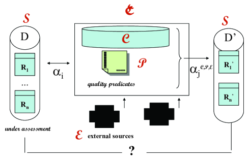
Figure 4: Contexts with External Sources

If the request for external data is performed without a value selection, then the external predicate might possibly return an unnecessarily large instance (of which only a portion would be used at the contextual level). Or the external source could return no data if it is not queried with the right access bindings (cf. below), a problem that has been investigated in data management [25, 30].

We now describe a way to address both problems that is based on properly pushing down value selections. That is, the evaluation can invoke the external predicates with some bounded variables, getting in return a much smaller answer set, namely the one satisfying the value selection. To do this, we make use of magic sets techniques (MST) [8], a family of bottom-up query evaluation methodologies that simulate the pushing-down of selections found in top-down approaches (cf. also [28, 1] for more details).

Example 7

(example 4 continued) To simplify the presentation, we will use instead of predicate ${\it\textbf{TempNoon'}}_{\!\!\!\mathcal{P}}$ defined in (3), a new (clean) alternative predicate, namely ${\it\textbf{TempNoon''}}_{\!\!\!\mathcal{P}}$, which is defined using only the ${\it Certified}$ CQP:

$$\textbf{TempNoon''}_{\!\mathcal{P}}(p,v,t,d) ~{}\leftarrow~{} {\it\textbf{M}(p,v,t,d,i)},\ \mbox{11:30}\leq t\leq\mbox{12:30},$$

$${\it Certified(p,d,t)}.$$

Furthermore, assume that ${\it Certified(p,d,t)}$ is now defined in terms of an external source ${\it\#\!C(Nurse,Year)}$, and not as in (27) in terms of the local source ${\it\textbf{C}(Nurse,Year)}$:

$${\it Certified(p,d,t)}\leftarrow{\it MNT(p,d,t,n,i,tp)},{\it\#\!C}(n,y).$$ (38)

Predicate ${\it MNT}$ was defined via (3)-(3) in Example 3. However, for the sake of illustration, we will assume in this example that it is an extensional (non-defined) predicate.

The external source ${\it\#\!C(Nurse,Year)}$ contains information about certified nurses; and ${\it\#\!C(Nurse,Year)}$ returns the year of certification if the input nurse appears in the source, and the constant ${\it null}$, otherwise. Furthermore, this source only returns an answer (the certification year) if it is asked about a specific nurse at a time. That is, the access to this source is subject to binding restrictions. It is not possible to obtain answers to queries about a whole set of unnamed nurses. $\blacksquare$

The first issue is, in general, how to guarantee that the binding restrictions are satisfied, i.e., to make sure that input attributes are always bound at the moment of requesting external data.

We address that issue by considering only input guarded rules:  for every rule $r$ (in a Datalog definition) containing an external predicate $\#E$ in its body, every input variable of $\#E$ (i.e. that requires a concrete instantiation in a query, like ${\it Nurse}$ in the example) has to appear in some previous atom in the body of $r$, but not as input variable for another external predicate. This condition can be used to guarantee that input variables in external predicates can be bound when the request for data is made.

Example 8

(example 7 continued)  In order to obtain quality answers to query (32), the query is rewritten, as expected, as

$$\mathcal{Q}^{\prime\prime}({\it p,v})\ \leftarrow\ \textbf{TempNoon''}_{\!\mathcal{P}}{\it(p,v,t,d)},\ d=\mbox{Sep/5}.$$ (39)

If we do a naive bottom-up evaluation, we will need to invoke ${\it\#\!C}$ for every nurse in ${\it MNT}$ as a bulk, which, apart from not being allowed by the source, could generate a huge amount of data.

Instead, by looking at the evaluation tree shown in Figure 5 for this Datalog query (each branching point corresponds to a conjunction), we can see that we would rather ask about nurses who were working on Sept/5.

We can also see from the query tree that the nurse name $n$ is not yet bound at the time of triggering the request for external data. In consequence, we have to make sure that both the date $d=\mbox{Sep/5}$ and the name are evaluated before we access the external source. $\blacksquare$

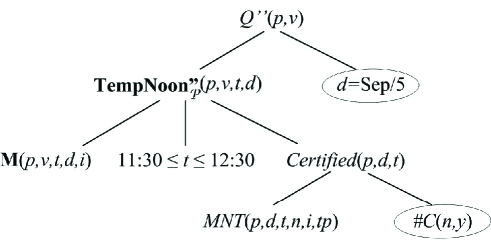
Figure 5: Parse tree for $\mathcal{Q}^{\prime\prime}({\it p,v})$

Top-down techniques use the value selection in the query to restrict the evaluation to facts that are relevant to the query. However, top-down methods are less appropriate that bottom-up approaches when a possibly large amount of data is involved [28]. By using the magic sets technique, the original Datalog query is rewritten into a new Datalog program, the magic program, for which the bottom-up evaluation focuses only on relevant facts (for the original query).

We will briefly summarize and use one of the variants of this methodology, the “generalized supplementary magic” [1, sec. 13.2-13.3]. The construction of the magic program is based on the notion of sideways information passing (SIP), according to which values are passed from one predicate to the next (from left to right in a rule body) during the evaluation of a rule body.

We begin by “adorning” each occurrence of a predicate in a rule of the original program with a label for each variable (or argument). Such a label indicates whether the variable is either bound ($b$) or free ($f$) at the time of the SIP evaluation. Each sequence of labels ($f$ or $b$) for a predicate is called an adornment. We describe the annotation process by means of our running example.

Example 9

(example 8 continued) The query in (39) is an open query, i.e. about all the tuples $(p,v)$ that satisfy the rule body. Then, the variables $p,v$ in the query predicate $\mathcal{Q}^{\prime\prime}$ are implicitly free ($f$); and the top predicate becomes annotated as $\mathcal{Q}^{\prime\prime f\!f}$.

The other predicates that appear in the program computing the query are also adorned, and the adorned versions of rules in Example 7 are as follows:

$$\mathcal{Q}^{\prime\prime f\!f}({\it p,v}) ~{}\leftarrow~{} d=\mbox{Sep/5},\textbf{TempNoon''}_{\!\!\mathcal{P}}^{{\it fffb}}{\it(p,v,t,d)}.$$

$$\textbf{TempNoon''}_{\!\!\!\mathcal{P}}^{\!{\it fffb}}\!(p,v,t,d) ~{}\leftarrow~{} {\it\textbf{M}(p,v,t,d,i)},\ \mbox{11:30}\leq t\leq\mbox{12:30},$$

$${\it Certified^{\!bbb}\!(p,d,t)}.$$

$${\it Certified^{\!bbb}\!(p,d,t)} ~{}\leftarrow~{} {\it MNT(p,d,t,n,i,tp)},{\it\#\!C^{\!bf}\!(n,y)}.$$

In the first rule, the selection for $d$ makes it become adorned with $b$ in the right-most predicate. The second rule is introduced with those adornments in the head, because that is the predicate we have to evaluate at the end of the body in the previous rule.

In rule (9), and in general, the extensional predicate is not annotated since the totality of data is just there, to be used without restriction. The last predicate in it has all its arguments adorned with $b$, because they all appear in a predicate to the left in the same rule body, whose evaluation will make them take specific values that will be used when the right-most predicate is processed.

The third rule is introduced to evaluate the last predicate in rule (9). As before, the right-most predicate in the body has its first argument, $n$, adorned with $b$, because its appears in a predicate to the left. $\blacksquare$

The process we just illustrated begins by adorning the query predicate (its head), and next its body. The bindings are then propagated to the other rules. Only intentional predicates are adorned; and we consider external predicates as special cases of intentional predicates since we do not have explicit extensions for them.

The adornment process is the first step. The resulting adorned program has now to be rewritten in terms of the so-called magic predicates, which is done as follows. For each rule $p\leftarrow a_{1},\ldots,a_{m}$ in the adorned program (excluding the query), we first create a new predicate $magic\_p$ containing only the bound arguments of $p$. Next, a supplementary relation ${\it sup}^{p}_{i}$ for each predicate $a_{i}$ is created. The arguments in ${\it sup}^{p}_{n}$ are those in the rule head. The arguments in ${\it sup}^{p}_{i}$, with $i\neq m$, contain all the arguments that occur in ${\it magic}\_p,a_{1},\ldots,a_{i},a_{i+1},\ldots,a_{m},{\it sup}^{p}_{m}$.

The rule above that defines $p$ is rewritten in terms of ${\it magic}\_p$ and ${\it sup}^{p}_{1},\ldots,$ ${\it sup}^{p}_{m}$, in such a way that can be used to simulate a SIP strategy with a bottom-up evaluation.

Example 10

(example 9 continued)  In the previous example we left having to evaluate predicates $\textbf{TempNoon''}_{\!\mathcal{P}}^{{\it fffb}}$ and ${\it Certified^{bbb}(p,}d,t)$ in the heads of the last two rules, resp. For this, we rewrite the rules for them using the magic and supplementary predicates, as follows:

$${\it\textbf{TempNoon''}}_{\mathcal{P}}^{{\it fffb}}(p,v,t,d) ~{}\leftarrow~{} {\it magic\!\_\textbf{TempNoon''}}_{\!\mathcal{P}}^{{\it fffb}}(d),\ {\it\textbf{M}(p,v,t,d,i)},$$

$${\it sup}^{1}_{1}(d,p,t),\ \mbox{11:30}\leq t\leq\mbox{12:30},{\it sup}^{1}_{2}(d,p,t),$$

$${\it Certified^{bbb}(p,d,t)},\ {\it sup}^{1}_{3}(p,v,t,d).$$

$${\it Certified^{bbb}(p,d,t)} ~{}\leftarrow~{} {\it magic\!\_Certified^{bbb}(p,d,t)},{\it MNT(p,d,t,n,i,tp)},$$

$${\it sup}^{2}_{1}(p,d,t,n),{\it\#\!\!C^{bf}(n,y)},{\it sup}^{2}_{2}(p,d,t).$$

According to our SIP strategy, predicates are evaluated from left to right. Consequently, ${\it magic\!\_\textbf{TempNoon''}}_{\!\mathcal{P}}^{{\it fffb}}$ will be initialized with the value $Sep/5$ taken from the query.

Next, considering the predicates by pairs, ${\it sup}^{1}_{1}$ will receive the result of the evaluation of ${\it magic\!\_\textbf{TempNoon''}}_{\!\mathcal{P}}^{{\it fffb}}$ and M. In its turn, ${\it sup}^{1}_{2}$ will get the result of the evaluation of ${\it sup}^{1}_{1}$ and $\mbox{11:30}\leq t\leq\mbox{12:30}$. Finally, ${\it sup}^{1}_{3}$ will receive the values from the evaluation of ${\it sup}^{1}_{2}$ and ${\it Certified^{bbb}}$.

Considering all this, we can rewrite the rule defining ${\it\textbf{TempNoon''}}_{\!\mathcal{P}}^{{\it fffb}}$ into a set of rules:

$${\it magic\!\_\textbf{TempNoon''}}_{\!\mathcal{P}}^{{\it fffb}}(d) ~{}\leftarrow~{} d=Sep/5.$$

$${\it sup}^{1}_{1}(d,p,t) ~{}\leftarrow~{} {\it magic\!\_\textbf{TempNoon''}}_{\!\mathcal{P}}^{{\it fffb}}(d),{\it\textbf{M}(p,v,t,d,i)}.$$

$${\it sup}^{1}_{2}(d,p,t) ~{}\leftarrow~{} sup^{1}_{1}(d,p,t),\mbox{11:30}\leq t\leq\mbox{12:30}.$$

$${\it sup}^{1}_{3}(p,v,t,d) ~{}\leftarrow~{} sup^{1}_{2}(d,p,t),{\it Certified^{bbb}(p,d,t)}.$$

$${\it\textbf{TempNoon''}}_{\!\mathcal{P}}^{{\it fffb}}(p,v,t,d) \leftarrow {\it sup}^{1}_{3}(p,v,t,d).$$

The rewriting for ${\it Certified^{bbb}}$ is similar:

$${\it magic\!\_Certified^{bbb}(p,d,t)} ~{}\leftarrow~{} {\it sup}^{1}_{2}(d,p,t).$$

$${\it sup}^{2}_{1}(p,d,t,n) ~{}\leftarrow~{} {\it magic\_Certified^{bbb}(p,d,t)},{\it MNT(p,d,t,n,i,tp)}.$$

$${\it sup}^{2}_{2}(p,d,t) ~{}\leftarrow~{} {\it sup}^{2}_{1}(p,d,t,n),{\it\#\!\!C^{bf}(n,y)},$$

$${\it Certified^{bbb}(p,d,t)} ~{}\leftarrow~{} {\it sup}^{2}_{2}(p,d,t).$$

Some predicates are redundant. In general, a supplementary predicate that appears with no other predicate in a rule’s body can be replaced by its definition. With that simplification, the resulting magic program for the original adorned rules of Example 9 becomes:

$${\it magic\!\_\textbf{TempNoon''}}_{\!\mathcal{P}}^{{\it fffb}}(d) ~{}\leftarrow~{} d=Sep/5.$$

$${\it sup}^{1}_{1}(d,p,t) ~{}\leftarrow~{} {\it magic\!\_\textbf{TempNoon''}}_{\mathcal{P}}^{{\it fffb}}(d),\ {\it\textbf{M}(p,v,t,d,i)}.$$

$${\it sup}^{1}_{2}(d,p,t) ~{}\leftarrow~{} {\it sup}^{1}_{1}(d,p,t),\mbox{11:30}\leq t\leq\mbox{12:30}.$$

$$\textbf{TempNoon''}_{\!\mathcal{P}}^{{\it fffb}}(p,v,t,d) ~{}\leftarrow~{} {\it sup}^{1}_{2}(d,p,t),{\it Certified^{bbb}(p,d,t)}.$$

$${\it magic\!\_Certified^{bbb}(p,d,t)} ~{}\leftarrow~{} {\it sup}^{1}_{1}(d,p,t),\mbox{11:30}\leq t\leq\mbox{12:30}.$$

$${\it sup}^{2}_{1}(p,d,t,n) ~{}\leftarrow~{} {\it magic\!\_Certified^{bbb}(p,d,t)},\ {\it MNT(p,d,t,n,i,tp)}.$$

$${\it Certified^{bbb}(p,d,t)} ~{}\leftarrow~{} {\it sup}^{2}_{1}(p,d,t,n),\ {\it\#C^{bf}(n,y)},$$

$$\mathcal{Q}^{M}({\it p,v}) ~{}\leftarrow~{} d=\mbox{Sep/5},\ \textbf{TempNoon''}_{\!\mathcal{P}}^{{\it fffb}}(p,v,t,d).$$

The last rule collects the (quality) answers to the query in (39).

The magic query program has the evaluation tree in Figure 6. We can use and follow it for a bottom-up evaluation of the query (predicate) at the root.

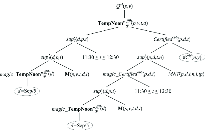
Figure 6: Parse tree for $\mathcal{Q}^{M}({\it p,v})$

This magic program and its bottom-up evaluation will take full advantage of the selections involved. Notice that, by the time we need to issue a data request to the external predicate $\#\!C$, the value selection $d=Sep/5$ has already been applied. That is, the external predicate will receive a restricted subset of names, those of the nurses that were working on $Sep/5$.

In fact, if we consider the subtree rooted at ${\it Certified}$, we notice that the value selection $d=Sep/5$ propagates upwards, and therefore $sup^{1}_{1}$, ${\it magic\!\_Certified}$, and $sup^{2}_{1}$ all receive only tuples corresponding to $Sep/5$. When the request for external data is issued, only three names are left: Susan, Cathy and Joan. Since predicate $\#C$ has the adornment $\#C^{bf}$, a specific query to $\#C$ for each of these 3 values is issued. In contrast, an evaluation based on the tree in Figure 5 would send a query to $\#\!C$ for all the nurse names appearing in relation ${\it MNT}$. $\blacksquare$

Having the possibility of taking into account the value selections involved in the query when evaluating it bottom-up is crucial for dealing with external sources. We want to be as restrictive as possible when querying them, while still producing the correct results.

Notice that in definition (38), we would expect to call $\#C$ always with a specific value for $n$. In other words, predicate $\#C$ should always have the binding $\#C^{bf}$. In the previous example, after applying the magic set (MS) methodology, it happened that this predicate got the right binding, obtaining a safe call to $\#C$. However, this raises the issue as to whether we can always guarantee that this will happen (possibly through a modified MS that is also guided by the initially given bindings).

We addressed this problem by assuming the input guarded condition. It guarantees that the right bindings for the external predicates are maintained after applying MS. More precisely, if the rule is input guarded, then every input variable of the external predicate $\#E$ also appears in some atom before it. Thus, by applying MS to a rule $p\leftarrow a_{1},\ldots,a_{n},\#E,a_{n+1},\dots,a_{m}$, we produce a set of rules for ${\it sup}^{p}_{i}$ that maintain the bindings. The reason for that is that the arguments of the ${\it sup}^{p}_{i}$ contain the variables that appear before and after them in $p$. In particular, they will contain the input variables of $\#E$.

Once we have the MS rewriting, the question is how to get data from the external sources given their access restrictions. We have seen how the input guarded condition guarantees the right bindings in terms of input/output parameters.

Our evaluation methodology has to implement the right access method, one that is compatible with the access restrictions as expressed via input/output parameters. This can be done by placing a trigger or active rule [64] in a DBMS at the contextual level, or through an application program running from the context. Either way, a procedure is needed that request the output values from external for given input values.

For example, we may have a defining rule containing an external source, say

$$\hskip 28.45274ptp(\bar{x}) ~{}\leftarrow~{} a_{1}(\bar{x}_{1}),\ldots,a_{j}(\bar{x}_{j}),\#E(i_{1},\ldots,i_{n},o_{1},\ldots,o_{m}),$$

$$a_{j+1}(\bar{x}_{j+1}),\dots,a_{k}(\bar{x}_{k}),$$

where $i_{1},\ldots,i_{n}$ are the input parameters and $o_{1},\ldots,o_{m}$ are the output parameters. Notice that $i_{1},\ldots,i_{n}$ appear in $\cup_{i=1}^{j}\bar{x}_{i}$.

In this case, we create a procedure ${\it get\#\!E}[I_{1},\ldots,I_{n};O_{1},\ldots,O_{m}]$, with the obvious input/output parameters. We may assume that the output values are null when the procedure is undefined for a particular combination of input values. Furthermore, assuming a SIP evaluation, we define a new predicate ${\it input(i_{1},\ldots,i_{n})}$ by:  ${\it input}(i_{1},\ldots,i_{n})\ \leftarrow\ a_{1}(\bar{x}_{1}),\ldots,a_{j}(\bar{x}_{j})$.

Every time a new tuple ${\it input}(c_{1},\ldots,c_{n})$ is created, while evaluating (10), the procedure is invoked as ${\it get\#\!E}[c_{1},\ldots,c_{n};O_{1},\ldots,O_{m}]$. The returned values are passed over to the predicates to the right.

Example 11

(example 10 continued)  In the magic program, the external predicate appears in the definition of ${\it Certified}$:

$${\it Certified^{bbb}(p,d,t)}\ \leftarrow\ {\it sup}^{2}_{1}(p,d,t,n),\ {\it\#C^{bf}(n,y)}$$

From this we define:  ${\it input}(n)\ \leftarrow\ {\it sup}^{2}_{1}(p,d,t,n)$; and create the procedure ${\it get\#\!C}[N;Y]$.

In this example, the procedure will be invoked once for each nurse name appearing as a value for ${\it input}$, in this case, those who worked on Sep/5, i.e. Susan, Cathy and Joan. Assuming that the (now) external source $\#C$ contains the information in Table 4, the external calls will produce ${\it get\#\!C[Susan;1996]}$, ${\it get\#\!C[Cathy;2009]}$, and ${\it get\#\!C[Joan;null]}$. $\blacksquare$

References

- [1] Abiteboul, S., Hull, R. and Vianu, V. Foundations of Databases. Addison-Wesley, 1995.
- [2] Anality, A., Theodorakis, M., Spyratos, N., Constantopoulos, P. Contextualization as an Independent Abstraction Mechanism for Conceptual Modeling. Information Systems, 2007, 32:24-60.
- [3] M. Arenas, J. Perez, J. Reutter, and C. Riveros. Composition and Inversion of Schema Mappings. SIGMOD Record, 2010, 38:17-28.
- [4] Arenas, M., Barcelo, P., Libkin, L. and Murlak, F. Relational and XML Data Exchange. Synthesis Lectures on Data Management, Morgan & Claypool Publishers, 2010.
- [5] Baldauf, M. A Survey on Context-Aware Systems. Int. J. Ad Hoc and Ubiquitous Computing, 2007, 2(4):263-277.
- [6] Ballou, D., Wang, R., Pazer, H. and Tayi, G. Modeling Information Manufacturing Systems to Determine Information Product Quality. Management Science, 44(4):462-484, 1998.
- [7] Batini, C. and Scannapieco, M. Data and Information Quality - Dimensions, Principles and Techniques. Data-Centric Systems and Applications, Springer, 2016.
- [8] Beeri, C. and Ramakrishnan, R. On the Power of Magic. Proc. SIGMOD 1987, pp. 269-284.
- [9] Bernstein, Ph. and Melnik, S. Model Management 2.0: Manipulating Richer Mappings. Proc. SIGMOD 2007, pp. 1-12.
- [10] Bertossi, L. and Bravo, L. Consistent Query Answers in Virtual Data Integration Systems. In Inconsistency Tolerance, Springer LNCS 3300, 2004, pp. 42-83.
- [11] Bertossi, L. and Bravo, L. Query Answering in Peer-to-Peer Data Exchange Systems. In Current Trends in Database Technology, Springer LNCS 3268, 2004, pp. 478-485.
- [12] Bertossi, L., Rizzolo, F. and Lei, J. Data Quality is Context Dependent. Proc. VLDB-WS on Enabling Real-Time Business Intelligence (BIRTE 2010). Springer LNBIP 48, 2011, pp. 52-67.
- [13] Bertossi, L. Database Repairing and Consistent Query Answering. Synthesis Lectures on Data Management, Morgan & Claypool, 2011.
- [14] Bertossi, L. and Bravo, L. Generic and Declarative Approaches to Data Quality Management. In S. Sadiq (ed.), Handbook of Data Quality - Research and Practice, Springer-Verlag, Berlin Heidelberg, 2013, pp. 181-212.
- [15] Bertossi, L. and Bravo, L. Consistency and Trust in Peer Data Exchange Systems. To appear in Theory and Practice of Logic Programming. doi:10.1017/S147106841600017X. 2016.
- [16] Bleiholder, J. and Naumann, F. Data Fusion. ACM Computing Surveys, 41(1):1-41, 2008.
- [17] Bolchini, C., Schreiber, F. and Tanca, L. A Methodology for a Very Small Data Base Design. Information Systems, 2007, 32(1):61-82.
- [18] Bolchini, C., Curino, C., Orsi, G., Quintarelli, E., Rossato, R., Schreiber, F. and Tanca, L. And What Can Context Do for Data? Communications of the ACM, 52(11):136-140, 2009.
- [19] Bolchini, C., Curino, C., Quintarelli, E., Schreiber, F. and Tanca, L. A Data-Oriented Survey of Context Models. SIGMOD Record, 36(4):19-26, 2007.
- [20] Bolchini, C., Quintarelli, E. and Rossato, R. Relational Data Tailoring Through View Composition. Proc. ER 2007, Springer LNCS 4801, pp. 149-164.
- [21] Bolchini, C., Curino, C., Quintarelli, E., Schreiber, F. and Tanca, L. Context Information for Knowledge Reshaping. Int. J. Web Eng. Technol., 2009, 5(1):88-103.
- [22] Bolchini, C., Quintarelli, E. and Tanca, L. CARVE: Context-Aware Automatic View Definition over Relational Databases. Information Systems, 2013, 38(1):45-67.
- [23] Bravo, L. and Bertossi, L. Logic Programs for Consistently Querying Data Integration Systems. Proc. IJCAI 2003, Morgan Kaufmann, pp. 10-15.
- [24] Brewka, G., Eiter, T. and Fink, M. Nonmonotonic Multi-Context Systems: A Flexible Approach for Integrating Heterogeneous Knowledge Sources. In Logic Programming, Knowledge Representation, and Nonmonotonic Reasoning, 2011, Springer LNCS 6565, pp. 233-258.
- [25] Cali, A. and Martinenghi, D. Querying Data under Access Limitations. Proc. ICDE 2008, pp. 50-59.
- [26] Cali, A., Gottlob, G. and Pieris, A. Towards more Expressive Ontology Languages: The Query Answering Problem. Artif. Intell., 2012, 193:87-128.
- [27] Cali, A., Gottlob, G., Lukasiewicz, T., Marnette, B., Pieris, A. Datalog+/-: A Family of Logical Knowledge Representation and Query Languages for New Applications. Proc. LICS 2010, pp. 228-242.
- [28] Ceri, S., Gottlob, G. and Tanca, L. Logic Programming and Databases. Springer, 1990.
- [29] De Giacomo, G., Lembo, D., Lenzerini, M. and Rosati, R. On Reconciling Data Exchange, Data Integration, and Peer Data Management. Proc. PODS 2007, pp. 133-142.
- [30] Deutsch, A., Ludäscher, B., and Nash, A. Rewriting Queries Using Views with Access Patterns under Integrity Constraints. Theor. Comput. Sci., 2007, 371(3): 200-226.
- [31] Duschka, O., Genesereth, M. and Levy, A. Recursive Query Plans for Data Integration. Journal of Logic Programming, 2000, 43(1):49-73.
- [32] Enderton, H. A Mathematical Introduction to Logic, 2nd Ed. Academic Press, 2001.
- [33] Fan, W. Dependencies Revisited for Improving Data Quality. Proc. PODS 2008, pp. 159-170.
- [34] Fan, W. and Geerts, F. Foundations of Data Quality Management. Synthesis Lectures on Data Management, Morgan & Claypool Publishers 2012
- [35] Frege. G. Über Sinn und Bedeutung. Zeitschrift für Philosophie und philosophische Kritik, NF 100, 1892, pp. 25-50.
- [36] Gay, G. Context-Aware Mobile Computing. Synthesis Lectures on Human-Centered Informatics # 4, Morgan & Claypool, 2009.
- [37] Ghidini, C. and Serafini, L. Model Theoretic Semantics for Information Integration. Proc. AIMSA 1998, Springer LNCS 1480, pp. 267-280.
- [38] Ghidini, C. and Giunchiglia, F. Local Models Semantics, or Contextual Reasoning = Locality + Compatibility. Artificial Intelligence, 2001, 127:221-259.
- [39] Giunchiglia, F. and Serafini, L. Multilanguage Hierarchical Logics. Artificial Intelligence, 1994, 65:29-70.
- [40] Giunchiglia, F. Contextual Reasoning. Proc. IJCAI-WS on Using Knowledge in its Context, 1993, pp. 39-49.
- [41] Grahne, G. and Mendelzon, A. O. Tableau Techniques for Querying Information Sources through Global Schemas. Proc. ICDT 1999. pp. 332-347.
- [42] Halevy, A. Answering Queries Using Views: A Survey. VLDB Journal, 2001, 10(4):270-294.
- [43] Hurtado, C., Gutierrez, C. and Mendelzon, A. Capturing Summarizability with Integrity Constraints in OLAP. ACM Transactions on Database Systems, 2005, 30(3):854 - 886.
- [44] Homola, M. and Serafini, L. Towards Formal Comparison of Ontology Linking, Mapping and Importing. In Proc. DL’10, CEUR-WS 573, 2010, pp. 291-302.
- [45] Imielinski, T. and Lipski Jr., W. Incomplete Information in Relational Databases. Journal of the ACM, 1984, 31(4):761-791.
- [46] Jiang, L., Borgida, A. and Mylopoulos, J. Towards a Compositional Semantic Account of Data Quality Attributes. Proc. ER 2008, Springer LNCS 5231, pp. 55-68.
- [47] Kivinen, J. and Mannila, H. Approximate Inference of Functional Dependencies from Relations. Theoretical Computer Science, 1995, 149:129-149.
- [48] Kolaitis, Ph. Schema Mappings, Data Exchange, and Metadata Management. Proc. PODS 2005, pp. 61-75.
- [49] Kontchakov, R., Lutz, C., Toman, D., Wolter, F. and Zakharyaschev, M. The Combined Approach to Query Answering in DL-Lite. Proc. KR 2010, pp. 247-257.
- [50] Lenzerini, M. Data Integration: A Theoretical Perspective. Proc. PODS 2002, pp. 233-246.
- [51] Maier, D., Ullman, J. and Vardi, M. On the Foundations of the Universal Relation Model. ACM Transactions on Database Systems, 1984, 9(2):283-308.
- [52] Martinenghi, D. and Torlone, R. Querying Context-Aware Databases. Proc. FQAS 2009, Springer LNCS 5822, pp. 76-87.
- [53] Martinenghi, D. and Torlone, R. Querying Databases with Taxonomies. Proc. ER 2010, Springer LNCS 6412, pp. 377-390.
- [54] Martinenghi, D. and Torlone, R. Taxonomy-Based Relaxation of Query Answering in Relational Databases. The VLDB Journal, 2014, 23(5):747-769.
- [55] McCarthy, J. Notes on Formalizing Context. Proc. IJCAI 1993, pp. 555-562.
- [56] Meliou, A., Gatterbauer, W., Halpern, J., Koch, Ch., Moore, K. and Suciu, D. Causality in Databases. IEEE Data Eng. Bull.. 2010, 33(3):59-67.
- [57] Milani, M. and Bertossi, L. Ontology-Based Multidimensional Contexts with Applications to Quality Data Specification and Extraction. In ’Rule Technologies: Foundations, Tools, and Applications’ (Proc. RuleML’15). Springer LNCS 9202, 2015, pp. 277-293.
- [58] Poggi, A., Lembo, D., Calvanese, D., De Giacomo, G., Lenzerini, M. and Rosati, R. Linking Data to Ontologies. Journal of Data Semantics, 2008, 10:133-173.
- [59] Naumann, F. Quality-Driven Query Answering for Integrated Information Systems. Springer, 2002.
- [60] Rajamaran, A. and Ullman, J. D. Mining of Masssive Datasets. Cambridge Univ. Press, 2012.
- [61] Reiter, R. Towards a Logical Reconstruction of Relational Database Theory. In On Conceptual Modelling, M.L. Brodie, J. Mylopoulos and J.W. Schmidt (eds.), Springer, 1984, pp. 191-233.
- [62] Reiter, R. What Should A Database Know? J. Logic Programming, 1992, 14:127-153.
- [63] Wang, R. and Strong, D. Beyond Accuracy: What Data Quality Means to Data Consumers. J. Management and Information Systems, 1996, 12(4):5-33.
- [64] Zaniolo, C., Ceri, S., Faloutsos, Ch., Snodgrass, R., Subrahmanian, V.S. and Zicari, R. Advanced Database Systems. Morgan Kaufmann Publishers, 1997.