WASP-86b and WASP-102b: super-dense versus bloated planets

We report the discovery of two transiting planetary systems: a super dense, sub-Jupiter mass planet WASP-86b ($M_{\rm pl}$ = 0.82 $\pm$ 0.06 M_J; $R_{\rm pl}$ = 0.63 $\pm$ 0.01 R_J), and a bloated, Saturn-like planet WASP-102b ($M_{\rm pl}$ = 0.62 $\pm$ 0.04 M_J; $R_{\rm pl}$ = 1.27 $\pm$ 0.03 R_J). They orbit their host star every $\sim$5.03, and $\sim$2.71 days, respectively. The planet hosting WASP-86 is a F7 star ($T_{\rm eff}$ = 6330$\pm$110 K, [Fe/H] = $+$0.23 $\pm$ 0.14 dex, and age $\sim$0.8–1 Gyr); WASP-102 is a G0 star ($T_{\rm eff}$ = 5940$\pm$140 K, [Fe/H] = $-$0.09$\pm$ 0.19 dex, and age $\sim$1 Gyr). These two systems highlight the diversity of planetary radii over similar masses for giant planets with masses between Saturn and Jupiter. WASP-102b shows a larger than model-predicted radius, indicating that the planet is receiving a strong incident flux which contributes to the inflation of its radius. On the other hand, with a density of $\rho_{\rm pl}$ = 3.24$\pm$ 0.3 $\rho_{\rm J}$, WASP-86b is the densest gas giant planet among planets with masses in the range 0.05 $<M_{\rm pl}<$ 2.0 M_J. With a stellar mass of 1.34 $M_{\odot}$ and [Fe/H]= $+$0.23 dex, WASP-86 could host additional massive and dense planets given that its protoplanetary disc is expected to also have been enriched with heavy elements. In order to match WASP-86b’s density, an extrapolation of theoretical models predicts a planet composition of more than 80% in heavy elements (whether confined in a core or mixed in the envelope). This fraction corresponds to a core mass of approximately 210M_⊕ for WASP-86b’s mass of $M_{\rm pl}$$\sim$260 M_⊕. Only planets with masses larger than about 2 M_J have larger densities than that of WASP-86b, making it exceptional in its mass range.

1 Introduction

We now know of more than 2500 planetary systems with single and multiple planets . Among these discoveries, the WASP sample represents an important contribution because WASP planets orbit bright stars which allow for precise follow-up photometric and spectroscopic observations. To date, the WASP survey (Pollacco et al. 2006) has discovered more than 160 planets, making it the most successful ground-based transit survey. We are now in the era of K2 (Howell et al. 2014), TESS (Ricker et al. 2015), and CHEOPS space missions hunting for Earth-like analogues. However, ground-based wide-fields surveys, such as WASP and HAT/HATS (Bakos et al. 2004, 2013) just to mention a few, are capable of detecting peculiar objects for example HATS-17 b, (Penev et al. 2016); HATS-18 b, (Brahm et al. 2016), increasing the spectrum of possible mass-radius relations in the planetary regime. These systems provide invaluable observational constraints on theoretical models.

Bright transiting systems are the only systems for which masses and radii can be derived with high precision, in turn providing insight into the planetary bulk composition via their estimated densities. The wide range of properties observed for the class of gas giant planets are still not fully understood. For example, the diversity in exoplanet densities and hence in their internal compositions is particularly noticeable at sub-Jupiter masses (0.05 $<M_{\rm pl}<$ 1M_J) where densities span 2 orders of magnitude. Systems like HD 149026b ($\rho_{\rm pl}\simeq 1\rho_{\rm J}$; Sato et al. 2005) and WASP-59b ($\rho_{\rm pl}\simeq 1.8\rho_{\rm J}$; Hébrard et al. 2013) are very dense planets in this mass range for which a rock/ice core of $\sim$70 $M_{\oplus}$ (corresponding to a heavy elements enrichment of $>60\%$) is hypothesised. At the opposite end of the spectrum we have planets like WASP-17b ($\rho_{\rm pl}=0.06\rho_{\rm J}$, Anderson et al. 2010b, 2011) and WASP-31b ($\rho_{\rm pl}=0.132\leavevmode\nobreak\ \rho_{\rm J}$, Anderson et al. 2010a), which are examples of planets with puzzling low densities. However, the planets in these systems are strongly irradiated. One of our latest discoveries is WASP-127b (Lam et al. 2016); with a mass of $\sim$3 times that of Neptune ($M_{\rm pl}=0.18\leavevmode\nobreak\ M_{\rm J}$) and a radius of 1.3$R_{\rm J}$ it is another example of an extremely low density planet ($\rho_{\rm pl}=0.068\rho_{\rm J}$). However its host star is a G0 and its orbital period is $\sim 4$ d implying that WASP-127b does not receive the same amount of flux as the two examples mentioned above. To assess the inflation status of a system, generally planetary radii are compared to theoretical models (e.g., Fortney et al. 2007; Burrows et al. 2007; Baraffe et al. 2008). However, the radius depends on multiple physical properties such as the stellar age, the irradiation flux, the planet’s mass, the atmospheric composition, the presence of heavy elements in the envelope or in the core, the atmospheric circulation, and also on any source generating extra heating in the planetary interior. Although models account for these contributions (e.g., tidal heating due to unseen companions pumping up the eccentricity Bodenheimer et al. 2001, Bodenheimer et al. 2003; kinetic heating due to the breaking of atmospheric waves Guillot & Showman 2002; enhanced atmospheric opacity Burrows et al. 2007; and semi-convection Chabrier et al. 2007), they can not explain the entire range of observed radii (Fortney & Nettelmann 2010; Leconte et al. 2010). This is not just the case for Jupiter-like gas giant planets, as even Neptune-like and smaller super-Earth planets show a large variety of properties which are difficult to reconcile with current knowledge of internal composition, structure, and formation histories (see for example Lissauer et al. 2014; Mayor et al. 2014).

In this paper, we present the discovery of two new transiting planetary systems from the WASP Survey: 1SWASP J175033.71+363412.7, hereafter WASP-86, and 1SWASP J222551.44+155124.5, hereafter WASP-102. WASP-86b and WASP-102b belong to the class of gas giant planets with sub-Jupiter masses. WASP-86b is the densest gas giant planet with a mass between that of Neptune and twice Jupiter’s mass, and shows similarities to both WASP-59b and HATS-17b. WASP-102b, in contrast, is a very bloated planet with a mass twice that of Saturn showing a radius anomaly similarly to WASP-17b and WASP-12b. Thus these SuperWASP discoveries provide new evidence of more extreme systems.

The paper is structured as follows: in $\S\ref{obs}$ and $\S\ref{rvobs}$ we describe the observations, including the WASP discovery data and follow-up photometric and spectroscopic observations which establish the planetary nature of the transiting objects. In §4 we present our results for the derived system parameters for the two systems, as well as the individual stellar and planetary properties. Finally in §5, we discuss the implication of these discoveries, their physical properties and how they extend the currently known mass-radius parameter space.

2 Photometric Observations

2.1 WASP Photometry

The SuperWASP telescope is located at the Roque de los Muchachos Observatory in La Palma (ING, Canary Islands, Spain). The telescope consists of 8 Canon 200mm f/1.8 lenses coupled to e2v 2048$\times$2048 pixel CCDs, which yield a field of view of $7.8\times 7.8$ square degrees with a corresponding pixel scale of 13$\aas@@fstack{\prime\prime}$7 (Pollacco et al. 2006). The SuperWASP observations have exposure times of 30 seconds, and a typical cadence of 8 min during the observing season. All WASP data are processed by the custom-built reduction pipeline described in Pollacco et al. (2006). The resulting light curves are analysed using our implementation of the Box Least-Squares and SysRem detrending algorithms (see Collier Cameron et al. 2006; Kovács et al. 2002; Tamuz et al. 2005) to search for transit-like features. Once the targets are identified as planet candidates a series of multi-season, multi-camera analyses are performed on the WASP photometry to strengthen the candidate’s detection. These additional tests allow a more thorough analysis of the stellar and planetary parameters, which are derived solely from the WASP data and publicly available catalogues (e.g., UCAC4; Zacharias et al. 2013), thus helping in the identification of the best candidates, as well as the rejection of possible spurious detections.

In the case of WASP-86, the WASP-North light curve consists of a total of 40223 data points that span from 2004 May 03 to 2010 August 24 (see top panel of Fig. 1). The WASP data show a dip in brightness characteristic of a transiting planet signal with a period of $P=5.031$ days, a transit duration of $\sim$4 hours, and a very shallow transit depth of 2.8 mmag. Given the very small signal of WASP-86b its detection is at the limit of the SuperWASP detection capability. Although the median photometric error of the WASP observations is of the same order of magnitude as the dip in brightness due to the planet, because of the multi-year span of the light curve and the large number of data points the transit signal is clearly significant in the periodogram (see Fig. 2). The periodogram is the result of the WASP analysis pipeline in which the Box-Least Squared periodogram is computed as per the prescription in Collier Cameron et al. (2006), and has been modified to fit multiple box widths. Thus, the reported $\Delta\chi^{2}$ is of the best epoch and best box-width combination.

The WASP-102 WASP-North light curve is comprised of 50126 photometric measurements spanning from 2004 June 23 to 2011 November 10 (see bottom Fig. 1). The transit signal in the WASP light curve is clearly detected, is periodic with a period $P\sim$2.71 d, and has a width of $\sim$3.5 hours and a depth of 10 mmag.

We omit the periodogram of WASP-102b in the paper, because the detection is more robust and has better follow-up photometry than WASP-86b which because of a much smaller radius and near-integer period as well as long transit duration has been elusive to acquire.

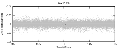
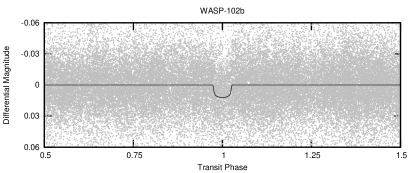
Figure 1: Discovery WASP Light Curves. Upper panel: WASP transit light curve of WASP-86b, phase folded on the ephemeris given in Table 7. The black, solid line is the MCMC best-fit transit model, as described in §4.3. Lower panel: Same as above in the case of WASP-102b.

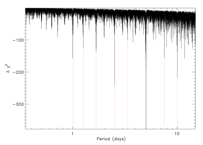
Figure 2: Box-Least Square periodogram of WASP-86b lightcurve. Period from the strongest feature is 5.03157 days and from the first MCMC run with only SuperWASP data is P = 5.03160 $\pm$ 0.00002 days. The orbital period of WASP-86b derived in §4.3 is the strongest feature in the periodogram; its aliases are marked by dotted-red lines (which from left to right are: P/5, P/4,P/3,P/2, 2P/3, 3P/2 and 2P).

Table 1: Photometric and astrometric properties of WASP-86 and WASP-102 from UCAC4 (Zacharias et al. 2013).

Parameter	WASP-86		WASP-102
${\rm RA(J2000)}$	17:50:33.718		22:25:51.447
${\rm Dec(J2000)}$	$+$36:34:12.79		$+$15:51:24.29
${\rm B}$	$11.33\pm 0.06$		$13.36\pm 0.03$
${\rm V}$	$10.66\pm 0.05$		$12.73\pm 0.02$
${\rm g}$	$...$		$13.06\pm 0.17$
${\rm r}$	$...$		$12.55\pm 0.04$
${\rm i}$	$...$		$13.11\pm 0.90$
${\rm J}$	$9.63\pm 0.02$		$11.49\pm 0.02$
${\rm H}$	$9.39\pm 0.02$		$11.22\pm 0.02$
${\rm K}$	$9.36\pm 0.02$		$11.11\pm 0.02$
$\mu_{\alpha}$ (mas/yr)	$-1.7\pm 1.0$		$-12.0\pm 2.0$
$\mu_{\delta}$ (mas/yr)	$-9.7\pm 0.7$		$-22.6\pm 2.6$

2.2 Follow-Up Multi-band Photometry

In this section, we describe the follow-up photometric observations for both systems. We note that given the long transit duration and the near integer orbital period a full transit light curve of WASP-86b has been difficult to acquire. All light curves will be available in the online version of the paper as electronic tables.

Table 2: Log of follow-up transit photometry observations.

Planet	Date	Tel./Inst.	Filter
WASP-86b	2013 07 16	FTN	Pan-STARRS-Z
	2014 04 23	NITES	no filter
	2014 08 27	LT	V$+$R
	2015 04 15	SPM	Johnson R
WASP-102b	2013 08 05	NITES	no filter
	2013 08 13	TRAPPIST	blue-blocking
	2013 08 13	EulerCam	Gunn-$r$
	2013 09 20	TRAPPIST	blue-blocking
	2013 09 20	EulerCam	Gunn-$r$
	2013 10 09	TRAPPIST	blue-blocking

Figure 3: Follow-up, high-precision, time-series photometry of WASP-86b during transit (see Table 2). The observations are shown as black points and are phase folded on the ephemeris shown in Table 7. The superimposed, solid, red line is our best-fit transit model (§4.3) using the formalism of Mandel & Agol (2002). The residuals from the fit and the individual data points photometric uncertainties are displayed directly under each light curve. Light curves and residuals are displaced from zero for clarity. In the right panel (SPM and LT light curves) given the density of the data and large uncertainties, we plot the average errorbar on the left of each light curve to avoid crowding.

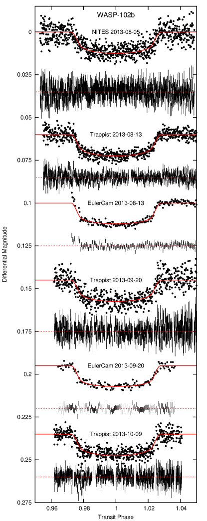
Figure 4: Follow-up, high signal-to-noise light curves of WASP-102b during transit. Same as Figure 3.

Faulkes North Telescope Observations. WASP-86 was observed with the 2-m Faulkes North Telescope in Hawai’i, USA on 2013 July 16, using the Spectral camera with a Pan-STARRS-Z filter. This has a Fairchild CCD486 BI detector with a pixel scale of 0.304 arcsec pixel^-1 in the (default) 2$\times$2 binning mode. The instrument was deliberately defocussed in order to spread the light over a larger number of pixels and to avoid saturation while executing 60s exposures, long enough to minimise noise due to scintillation. The data were pre-processed using the standard LCOGT 2-m reduction pipeline in use at the time, since these data were acquired prior to the 2-m telescopes being fully integrated with the larger LCOGT network. Aperture photometry was then conducted using a stand-alone implementation of DAOPHOT Stetson (1987).

NITES Observations. The Near Infra-red Transiting ExoplanetS (NITES) Telescope is a semi-robotic $0.4$-m (f/10) Meade LX200GPS Schmidt-Cassegrain telescope installed at the Observatorio del Roque de los Muchachos, La Palma, Spain. The telescope is mounted with Finger Lakes Instrumentation Proline 4710 camera, containing a $1024\times 1024$ pixels deep-depleted CCD made by e2v. The telescope has a field of view of $11\times 11$ arcmin squared and a pixel scale of 0.66 arcsec pixel^-1, respectively, and a peak QE$>90\%$ at $800$ nm. For more details on the NITES Telescope we refer the reader to McCormac et al. (2014).

One transit of WASP-86 b was observed on 2014 April 23. The telescope was defocused slightly to 7.3 arcsec (FWHM) and $587$ images of $20$ s exposure time were obtained with $5$ s dead time between each. The dead time is a combination of the CCD readout and an additional dwell time to allow for science frame autoguiding using the DONUTS algorithm (McCormac et al. 2013). One transit of WASP-102 b was observed on 2013 August 05. The telescope was defocused slightly to 3.3 arcsec and $827$ images of $20$ s exposure time were obtained with $5$ s dead time between each.

In order to obtain the best signal-noise ratio (SNR) both observations were made without a filter. The data were bias subtracted and flat-field corrected using PyRAF and the standard routines in IRAF and aperture photometry was performed using DAOPHOT (Stetson 1987). A total of $5$ and $6$ nearby comparison stars were used and aperture radii of $12\arcsec$ and $4\arcsec$ were chosen as they returned the minimum RMS scatter in the out of transit data for WASP-86 b and WASP-102 b, respectively. Initial photometric error estimates were calculated using the electron noise from the target and the sky, and the read noise within the aperture.

San Pedro Mártir Observations. The transit of WASP-86b was observed with the 84cm Telescope at the Observatorio Astronómico Nacional de San Pedro Mártir (SPM) in Baja California, México on 2015 April 15 (UT) using the Marconi 3 CCD and MEXMAN filter wheel. The images were binned 2$\times$2. The telescope was defocussed such that the exposure times were 60 s to maximise time on target and minimise the effects of the shutter, read out and scintillation. A total of 258 photometric data points using the Johnson R filter were acquired. We also observed the WASP-86b transit on 2015 April 11 with the same configuration; however due to clouds and the shallowness of the WASP-86 transits, the data were not sufficiently good to include in the analysis. The data were reduced and the light curves extracted following the standard procedures described in §2.2: NITES Observations.

TRAPPIST Observations. Three transits of WASP-102b were observed with the 0.6-m TRAPPIST robotic telescope (TRAnsiting Planets and PlanetesImals Small Telescope), located at ESO La Silla Observatory, Chile. TRAPPIST is equipped with a thermoelectrically-cooled 2K$\times$2K CCD, which has a pixel scale of 0.65″ that translates into a 22′$\times$22′ field of view. For details of TRAPPIST, see Gillon et al. (2011) and Jehin et al. (2011). The TRAPPIST photometry was obtained using a readout mode of 2$\times$2 MHz with 1$\times$1 binning, resulting in a readout plus overhead time of 6.1 s and a readout noise of 13.5 e^-. A slight defocus was applied to the telescope to improve the duty cycle, spread the light over more pixels, and, thereby improve the sampling of the point-spread function (PSF). The transits were observed in a blue-blocking filter that has a transmittance $>90\%$ from 500 nm to beyond 1000 nm. During the runs, the positions of the stars on the chip were maintained to within a few pixels thanks to a ”software guiding” system that regularly derives an astrometric solution for the most recently acquired image and sends pointing corrections to the mount if needed. After a standard reduction (bias, dark, and flat-field correction), the stellar fluxes were extracted from the images using the IRAF/ DAOPHOT aperture photometry software (Stetson 1987). For each light curve we tested several sets of reduction parameters and kept the one giving the most precise photometry for the stars of similar brightness as the target. After a careful selection of reference stars, the transit light curves were finally obtained using differential photometry.

EulerCam Observations. We observed two transits of WASP-102 using EulerCam mounted on the 1.2-m Swiss Telescope at ESO La Silla, Chile (Lendl et al. 2012). On 2013 August 13, we used an Gunn-r^′ filter and 80 s exposure times, obtaining 182 images with stellar FWHM between 1.15″ and 1.9″; while on 2013 September 20, we observed through a Cousins-I filter obtaining 123 120s exposures with FWHM between 1.9$\arcsec$ and 5.05$\arcsec$. All data were reduced as outlined in Lendl et al. (2012), and we performed aperture photometry with apertures of 5.05″(2013 Aug 13) and 9.45″(2013 Sep 20), for the first and second transit light curve, respectively. We carefully selected the most stable field stars as reference stars for the relative differential photometry such that the scatter in the light curves was minimised.

3 Spectroscopic Observations

WASP-86 and -102 were observed during our follow-up campaigns between 2012 May 16 and 2015 November 8 by means of the SOPHIE spectrograph mounted at the 1.93-m telescope (Perruchot et al. 2008; Bouchy et al. 2009) at Observatoire de Haute-Provence (OHP). In addition, WASP-102 was observed between 2012 September 15 and 2014 August 19 with the CORALIE spectrograph mounted at the 1.2-m Euler Swiss telescope at La Silla, Chile (Baranne et al. 1996; Queloz et al. 2000; Pepe et al. 2002).

The SOPHIE observations were obtained in high efficiency mode (R = 40 000), with very similar signal-to-noise ratio ($\sim$30), in order to minimise systematic errors (e.g., the charge transfer inefficiency effect of the CCD, Bouchy et al. 2009). Wavelength calibration with a thorium-argon lamp was performed every $\sim$2 hours, allowing for interpolation of the spectral drift of SOPHIE ($<$3 m s^-1per hour; see Boisse et al. 2010). Two 3$\arcsec$ diameter optical fibers were used; the first centered on the target and the second on the sky to simultaneously measure the background to remove contamination from scattered moonlight. The contamination of the CCF from scattered moonlight was negligible for most of the SOPHIE exposures because the Moon was low and/or well shifted from the targets’ radial velocity (RV) measurements. In some cases however there was a significant contamination which was corrected using the second SOPHIE aperture. The maximum corrections were 250 m s^-1 for WASP-86, and 160 m s^-1 for WASP-102.

The CORALIE observations of WASP-102 were obtained during grey/dark time to minimise moonlight contamination. Both SOPHIE and CORALIE data-sets were processed with standard data reduction pipelines. The radial velocity uncertainties were evaluated including known systematics such as guiding and centering errors (Boisse et al. 2010), and wavelength calibration uncertainties. All spectra were single-lined. In addition to the radial velocity variation of WASP-86b, the SOPHIE data show a linear drift which we have been monitoring. With the current phase coverage of SOPHIE data we can not yet put constraints on the mass of the secondary object which could be in the planetary regime.

For each planetary system the radial velocities were computed from a weighted cross-correlation of each spectrum with a numerical mask of spectral type G2, as described in Baranne et al. (1996) and Pepe et al. (2002). To test for possible stellar impostors we performed the cross-correlation with masks of different stellar spectral types (e.g., F0, K0 and K5). For each mask, we obtained similar radial velocity variations, thus rejecting a blended eclipsing system of stars with unequal masses as a possible cause of the variation.

We present in Tables 3 and 4 the spectroscopic measurements of WASP-86 and 102. In each table we list the Barycentric Julian date (BJD-TDB), the stellar radial velocity measurements, their uncertainties, the bisector span measurements (V_span), and the residuals to the best-fit Keplerian model; additionally in the case of WASP-102, we list the instrument used.

In Figure 5 we plot the phase folded radial velocity curve for WASP-86 (left) and WASP-102 (right). Additionally, the RV residuals from our best fit model are plotted against orbital phase (Figure 5: lower–panel). The $RMS$ of the residuals to the best fit Keplerian models are as follows: $RMS=30$ ms^-1 for WASP-86, and $RMS=15$ ms^-1 for WASP-102, which are comparable to the errors in the RV measurements. The systemic velocity and the long-term trend ($d\gamma/dt$) have been subtracted from the RVs, which in the case of WASP-86 are $\gamma$ = $-$23.676 $\pm$ 0.015 km s^-1 and  $d\gamma/d$ = 30.2$\pm$2.7 m s^-1 $y^{-1}$, and in the case of WASP-102 are $\gamma_{\rm\tiny SOPHIE}$ = $-$16.54584 $\pm$ 0.00064 km s^-1, $\gamma_{\rm\tiny CORALIE}$ = $-$16.5459 $\pm$ 0.00064 km s^-1 and $d\gamma/dt$ = 0. In Figure 6 we plot the bisector span measurements (V_span) for both systems versus radial velocity. The bisector span measurements of both planet hosts are of the same order of magnitude as the errors in the RV measurements, and show no significant variation nor correlation with radial velocity, as indicated by the Pearson product-moment correlation coefficient, $r$, see Figure 6. This suggests that the radial velocity variations with semi-amplitudes of $K_{1}$ = 0.0845 $\pm$0.0052 km s^-1 for WASP-86b, and $K_{1}$ = 0.0855 $\pm$0.0049 km s^-1 for WASP-102b, are due to Doppler shifts of the stellar lines induced by a planetary companion rather than stellar profile variations due to stellar activity or a blended eclipsing binary.

In the radial velocity signal of WASP-86b there is indication of an additional body in the system. Our current RV dataset does not allow us to confirm a third object nor to put constraints on its mass, but our analysis of the RV signal and bisector allow us to exclude relatively massive stellar companions.

Table 3: Radial velocity measurements of WASP-86 obtained with SOPHIE. The columns are: the Baricentric Julian date (BJD-TDB), the stellar RV measurements, the RV uncertainties, the line-bisector span measurements and the residuals to the fit.

BJD	RV	$\sigma_{\rm RV}$	Vspan	O – C
$-$2 400 000	(km s-1)	(km s-1)	(km s-1)	(m s-1)
56063.5320	$-$23.800	0.018	$-$0.028	$-$7.5
56066.4192	$-$23.659	0.018	$-$0.102	$-$13.3
56081.6018	$-$23.685	0.021	$-$0.068	$-$35.3
56084.4756	$-$23.778	0.008	$-$0.041	$-$29.0
56089.5905	$-$23.798	0.017	$-$0.008	$-$56.8
56101.3934	$-$23.657	0.016	$+$0.004	$-$22.2
56103.3771	$-$23.821	0.017	$-$0.071	$-$37.8
56121.3528	$-$23.666	0.021	$-$0.040	$-$34.3
56123.3949	$-$23.817	0.018	$+$0.027	$-$40.0
56125.3998	$-$23.707	0.017	$-$0.061	$-$24.4
56865.3807	$-$23.619	0.017	$-$0.031	$-$3.2
56939.2511	$-$23.777	0.017	$-$0.098	$-$35.2
56940.2622	$-$23.617	0.018	$-$0.112	$+$47.1
56948.2628	$-$23.715	0.017	$+$0.027	$-$2.7
56949.2668	$-$23.731	0.017	$-$0.040	$+$11.7
56950.3063	$-$23.698	0.017	$+$0.050	$-$32.5
56974.2357	$-$23.714	0.041	$-$0.118	$+$30.6
56974.2434	$-$23.785	0.021	$-$0.039	$-$40.4
56975.2256	$-$23.695	0.021	$-$0.153	$-$7.6
56977.2482	$-$23.606	0.017	$-$0.025	$-$2.0
56978.2316	$-$23.690	0.017	$-$0.003	$+$1.4
56979.2545	$-$23.779	0.018	$+$0.019	$-$34.6
56981.2452	$-$23.666	0.018	$-$0.064	$-$65.1
57107.5714	$-$23.587	0.018	$-$0.001	$-$7.2
57133.5154	$-$23.653	0.016	$-$0.092	$-$35.9
57134.4998	$-$23.723	0.017	$+$0.016	$-$15.1
57154.4733	$-$23.698	0.017	$+$0.016	$-$3.6
57158.5529	$-$23.603	0.019	$-$0.137	$+$3.1
57190.4498	$-$23.773	0.017	$+$0.010	$-$40.2
57191.4466	$-$23.719	0.017	$+$0.040	$-$30.4
57210.4813	$-$23.735	0.017	$-$0.032	$-$5.0
57211.4407	$-$23.679	0.017	$-$0.136	$+$19.8
57335.2876	$-$23.678	0.015	$-$0.016	$-$23.3

Table 4: Radial velocity measurements of WASP-102. The columns are: the Baricentric Julian date (BJD-TDB), the stellar RV measurements, the RV uncertainties, the line-bisector span measurements, the residuals to the fit and the instrument with which the observations were acquired (S = SOPHIE; C = CORALIE)

BJD	RV	$\sigma_{\rm RV}$	Vspan	O – C	Inst.
$-$2 400 000	(km s-1)	(km s-1)	(km s-1)	(m s-1)
56186.4885	$-$16.609	0.013	$-$0.037	$-$12.4	S
56187.5411	$-$16.460	0.014	$-$0.037	$+$2.3	S
56188.4985	$-$16.621	0.013	$-$0.001	$-$9.7	S
56192.4438	$-$16.514	0.013	$-$0.019	$-$16.9	S
56195.4307	$-$16.470	0.016	$+$0.006	$-$5.5	S
56213.4903	$-$16.601	0.013	$-$0.021	$+$9.5	S
56214.4346	$-$16.463	0.014	$+$0.003	$-$0.4	S
56216.3941	$-$16.572	0.021	$+$0.019	$+$7.9	S
56270.3117	$-$16.575	0.022	$-$0.077	$+$45.1	S
56271.2903	$-$16.468	0.016	$-$0.039	$-$2.4	S
56272.3265	$-$16.572	0.018	$-$0.023	$+$12.2	S
56285.2449	$-$16.463	0.017	$+$0.001	$+$10.9	S
56301.2458	$-$16.469	0.025	$-$0.023	$-$9.0	S
56302.2248	$-$16.597	0.023	$-$0.000	$+$2.2	S
56536.7314	$-$16.382	0.059	$+$0.107	$+$29.5	C
56538.6544	$-$16.555	0.044	$+$0.012	$-$8.5	C
56540.7007	$-$16.597	0.112	$-$0.091	$-$61.1	C
56543.6393	$-$16.554	0.017	$+$0.036	$+$6.6	C
56544.6662	$-$16.379	0.042	$-$0.104	$+$61.3	C
56545.6756	$-$16.463	0.017	$+$0.028	$-$9.7	C
56547.6195	$-$16.394	0.018	$+$0.040	$+$11.9	C
56550.6624	$-$16.388	0.025	$+$0.058	$+$9.1	C
56595.5549	$-$16.575	0.018	$+$0.023	$-$27.3	C
56599.5259	$-$16.390	0.028	$+$0.041	$+$12.5	C
56888.7397	$-$16.458	0.018	$-$0.029	$-$4.3	C

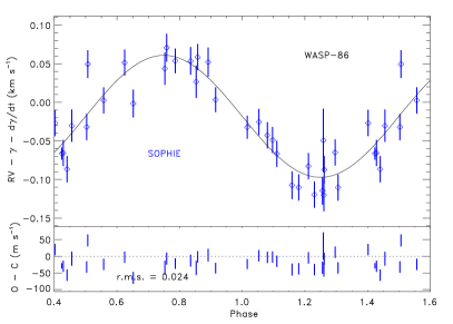
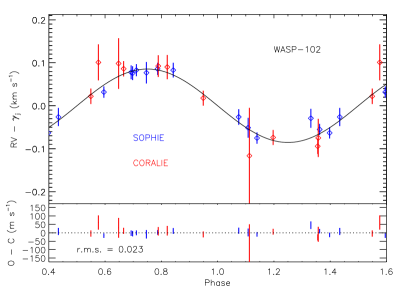
Figure 5: Upper panels: Phase folded relative radial velocity measurements of WASP-86 (left) and WASP-102 (right) obtained with the SOPHIE (blue) and CORALIE (red) spectrographs. The systemic velocity and the long-term trend ($d\gamma/dt$) have been subtracted from the RVs. Superimposed is the best-fit model RV curve with parameters from Table 7. Lower panels: Residuals from the radial velocity fit plotted against orbital phase; the dotted line in the lower panels marks zero. The residuals are in units of m s^-1. The r.m.s. are in units of km s^-1.

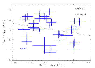
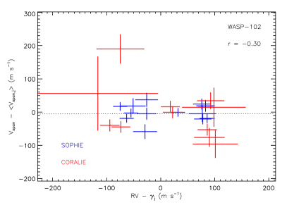
Figure 6: We plot the bisector span measurements of WASP-86 (left) and WASP-102 (right) as a function of relative radial velocity. From the bisector span value we subtract the mean bisector span for each instrument while removing the systemic velocity and in the case of WASP-86 the RV long-term trend ($d\gamma/dt$). In the case of WASP-86, $<$V${}_{\rm span}>$ = -36.9 m s^-1, and in the case of WASP-102, $<V_{\rm span,SOPHIE}>$ = -18.1 m s^-1 and $<V_{\rm span,CORALIE}>$ = 11.1 m s^-1. The horizontal, dotted line denotes the best linear fit to all of the data points including the individual uncertainties. The V_span measurements of both stars are of the same order of magnitude as the errors in the RVs, and show no significant variation nor correlation with RVs, as indicated by the Pearson product-moment correlation coefficient, $r$.

4 Physical Properties

We performed our routine analysis on the complete set of spectroscopic and photometric data for both systems, from which we derive stellar and planetary physical properties.

4.1 Spectroscopically-determined stellar properties

The stellar spectroscopic properties for WASP-86 and WASP-102 were obtained using the co-added spectra from SOPHIE and the methods given in Doyle et al. (2013). The excitation balance of the Fe i lines was used to determine the effective temperature ($T_{\rm eff}$). The surface gravity ($\log g$) was determined from the ionisation balance of Fe i and Fe ii. The Ca i line at 6439Å and the Na i D lines were also used as $\log g$ diagnostics. Values of microturbulence ($\xi_{\rm t}$) were obtained by requiring a null-dependence on abundance with equivalent width. The elemental abundances were determined from equivalent width measurements of several unblended lines. The quoted error estimates include that given by the uncertainties in $T_{\rm eff}$ and $\log g$, as well as the scatter due to measurement and atomic data uncertainties. The projected stellar rotation velocity ($v\sin i$) was determined by fitting the profiles of several unblended Fe i lines. Macroturbulence was obtained from the calibration by Bruntt et al. (2010). The overall precision of the parameters was limited by the quite modest signal-to-noise ratios of the spectra $\sim$80:1 for WASP-86 and $\sim$60:1 for WASP-102.

For WASP-86, the rotation rate ($P_{\rm rot}=5.7\pm 0.8$ d) implied by the $v\sin i$ gives a gyrochronological age of $0.8^{+0.8}_{-0.4}$ Gyr using the Barnes (2007) relation. The effective temperature of this star is close to the lithium-gap, (Böhm-Vitense 2004), thus the lack of any detectable lithium does not provide a usable age constraint. WASP-86’s rotation period, albeit assuming that the stellar rotation axis is along the plane of the sky, is remarkably close (within 1–$\sigma$ from $v\sin i$) to the orbital period of WASP-86b P = 5.03 days. Using the long baseline of WASP data (covering $\sim$6 yrs) we have investigated the presence of photometric modulation in the WASP light curve due to stellar variability. However, we do not detect any variation down to 0.5 mmag (see also §2.1 and Fig. 2). A more detailed analysis of the spectrum revealed no sign of stellar activity with a S/N of about 20:1 in the core of the Ca II H&K lines. The stellar mass and radius were estimated using the calibration of Torres et al. (2010).

In the case of WASP-102, the rotation rate ($P_{\rm rot}=8.1\pm 1.5$ d) implied by the $v\sin i$ gives a gyrochronological age of $0.6^{+0.5}_{-0.3}$ Gyr using the Barnes (2007) relation. An estimated lithium age of $\sim$0.5–2 Gyr estimated using Sestito & Randich (2005) is consistent. As in the case of WASP-86, there is no indication of stellar activity for WASP-102.

Table 5: Stellar Parameters from spectral analysis.

Parameter	WASP-86	WASP-102
$T_{\rm eff}$(K)	6330$\pm$110	5940$\pm$140
$\log g$	4.28$\pm$0.10	4.49$\pm$0.11
[Fe/H]	+0.23$\pm$0.14	+0.09$\pm$0.19
$\xi_{\rm t}$(km s-1)	1.1$\pm$0.2	1.0$\pm$0.2
$v_{\rm mac}$(km s-1)	4.3$\pm$0.3	3.0$\pm$0.3
$v\sin i$(km s-1)	12.1$\pm$0.8	6.2$\pm$0.7
$\log A$(Li)	$<$1.08	2.44$\pm$0.12
Mass (M⊙)	1.32$\pm$0.11	1.10$\pm$0.10
Radius (R⊙)	1.36$\pm$0.18	1.00$\pm$0.14
Sp. Type	F7	G0
Age	$0.8^{+0.8}_{-0.4}$ Gy	$0.6^{+0.5}_{-0.3}$ Gyr

Notes: Macroturbulence ($v_{\rm mac}$) was obtained from the calibration by Bruntt et al. (2010). The mass and radius were obtained using the Torres et al. (2010) calibration. The spectral type is estimated from $T_{\rm eff}$ using the table in Gray (2008). The iron abundance is relative to the solar value obtained by Asplund et al. (2009).

4.2 Stellar masses and ages

For both systems we used stellar theoretical evolutionary models in order to estimate stellar ages and masses. We used the stellar densities $\rho_{\star}$, measured directly from our Markov-Chain Monte Carlo (MCMC) analysis (§4.3, and see also Seager & Mallén-Ornelas 2003), together with the stellar temperatures and metallicity values derived from spectroscopy, to perform an interpolation over three different stellar evolutionary models. For details of the interpolation method see Brown (2014).

The stellar density, $\rho_{\star}$, is directly determined from transit light curves and as such is independent of the effective temperature determined from the spectrum (Hebb et al. 2009), as well as of theoretical stellar models (if $M_{\rm pl}\ll M_{\star}$ is assumed). The following stellar models were used: a) the Padova stellar models (Marigo et al. 2008, and Girardi et al. 2010), b) the Yonsei-Yale (YY) models (Demarque et al. 2004), and c) models from the Dartmouth Stellar Evolution Program (DSEP) (Chaboyer et al. 2001,Bjork & Chaboyer 2006, Dotter et al. 2008).

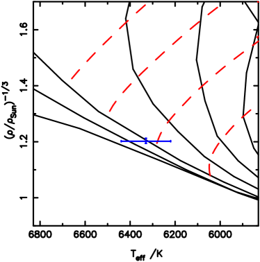
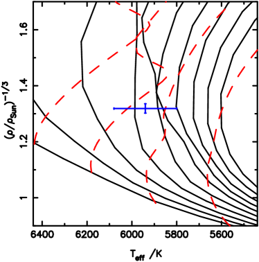
Figure 7: Isochrone tracks from Demarque et al. (2004) for WASP-86 and WASP-102 using the metallicity [Fe/H]$=+0.23$ dex and [Fe/H]$=+0.09$ dex respectively from our spectral analysis and the best-fit stellar density $\rho_{\star}$. Left-panel: WASP-86, from left to right the solid lines are for isochrones of: 0.1, 0.6, 1, 2, 3, and 4 Gyr. From left to right, dashed lines are for mass tracks of: 1.4, 1,3, 1.2, and 1.1 M_⊙. Right-panel: WASP-102, from left to right the solid lines are for isochrones of: 1, 2, 3, 4, 5, 6, 7, 8, 9, and 10 Gyr. From left to right, red–dashed lines are for mass tracks of: 1.3, 1.2. 1.1. and 1.0 M_⊙.

In Figure 7 we plot the inverse cube root of the stellar density $\rho_{\star}$${}^{-1/3}=$ $R_{\star}$/$M_{\star}$^1/3 (solar units) against effective temperature, $T_{\rm eff}$, for the selected model mass tracks and isochrones for the two planet host stars respectively. For WASP-86 the stellar properties derived from the three sets of stellar evolution models (Table 6) agree with each other, and with those derived from the Torres et al. (2010) calibration, within their 1–$\sigma$ uncertainties.

This is not the case for WASP-102 for which the stellar ages derived from theoretical models are quite different from the age obtained via gyrochronology see Table 6. In §4.1 from $v\sin i$ and using Barnes (2007) relation we obtained for WASP-102 an estimated stellar rotation period of about 8 days. For a G0 star this translate to an age of $\sim$0.6 Gyr. Moreover, the age estimate from the lithium abundance also suggests a young age (0.5–2 Gyrs). These values are in disagreement with the three evolutionary model estimates obtained above. Their 1–$\sigma$ lower limits seem to indicate an age of 2.6 Gyrs or older. However, we note that these values are fairly unconstrained and have large errors. Additionally, different sets of theoretical models might not perfectly agree with each other (Southworth 2010), and moreover at younger ages isochrones are closely packed and a small change in $T_{\rm eff}$ or $\rho_{\star}$ can have a significant effect on the derived stellar age. This is visible in Figure 7 where at young stellar ages isochrones are practically indistinguishable.

In principle, isochrone fitting is applicable to stars across the spectral range, but it can be difficult to determine ages for stars with spectral type later than mid-to-late G owing to the fact that they evolve very slowly, having nuclear burning time-scales that are longer than the age of the Galactic disc. Given our error on the $T_{\rm eff}$, [Fe/H] and $\rho_{\star}$ this could possibly explain the age discrepancy of WASP-102.

Even with precise stellar densities problem can arise. Grids of stellar models use a broad sampling in mass, age and metallicity that can produce poor sampling of the observed parameter spacing. In such a case the difference in stellar density between adjacent grid points can be much larger than the uncertainty on the observed value. This can produce systematic interpolation errors and make reliable estimates of the uncertainties on the mass and age difficult. Moreover, some combinations of mass, age and composition could be missed because are not sampled by the stellar model grid or fall just outside the 1–$\sigma$ error bars, particularly when fitting by-eye.

To avoid any such problem we have used the approach of Maxted et al. (2015b) to evaluate the masses and ages for both systems. Maxted et al. (2015b) developed a Markov-Chain Monte Carlo (MCMC) method (BAGEMASS), a Bayesian method that calculates the posterior probability distribution for the mass and age of a star from its observed mean density and other observable quantities (e.g. $T_{\rm eff}$, [Fe/H] and luminosity) using a grid of stellar models that densely samples the relevant parameter space. In Table 6 and Figure 8 we show the masses and ages obtained with this method. The results from BAGEMASS confirm a young age for WASP-86 of about 1.2$\pm$0.8 Gyr, and also find a mass estimate for WASP-86 (1.31$\pm$0.06 M_⊙) in agreement with our previous estimate. For WASP-102 instead we obtain an older age (5$\pm$2 Gyr) compared to gyrochonology in agreement with our previous estimate from stellar models, while the estimated stellar mass of 1.17$\pm$0.09 M_⊙ is in agreement with that derived from stellar models above and that from empirical calibrations (e.g. Torres et al. 2010).

Table 6: Stellar masses and ages for WASP-86 and WASP-102.

	WASP-86		WASP-102
	$M_{\star}$ (M⊙)	Age (Gyr)	$M_{\star}$ (M⊙)	Age (Gyr)
Padovaa	1.29${}^{+0.04}_{-0.09}$	0.52${}^{+1.54}_{-0.46}$	1.12${}^{+0.10}_{-0.15}$	5.35${}^{+5.35}_{-2.16}$
YYb	1.31${}^{+0.08}_{-0.08}$	1.05${}^{+1.16}_{-0.84}$	1.18${}^{+0.04}_{-0.19}$	4.45${}^{+4.85}_{-1.76}$
DSEPc	1.21${}^{+0.07}_{-0.05}$	2.72${}^{+0.80}_{-1.38}$	1.08${}^{+0.16}_{-0.15}$	6.49${}^{+4.98}_{-3.05}$
BAGEMASSd	1.31$\pm$0.06	1.2$\pm$0.8	1.17$\pm$0.09	5$\pm$2

^a Marigo et al. (2008); Girardi et al. (2010); ^b Demarque et al. (2004); ^c Chaboyer et al. (2001); Bjork & Chaboyer (2006); Dotter et al. (2008) ; ^d Maxted et al. (2015a)

Finally, considering the possible range of ages within the 1–$\sigma$ uncertainties we adopted an age of 1.2$\pm 0.8$ Gyr and 5$\pm 2$ Gyr for WASP-86 and WASP-102, respectively. In Figures 8, we show for each planet host star a plot with the chosen set of stellar models from Maxted et al. (2015a), while we give a comprehensive list of all models results in Table 6.

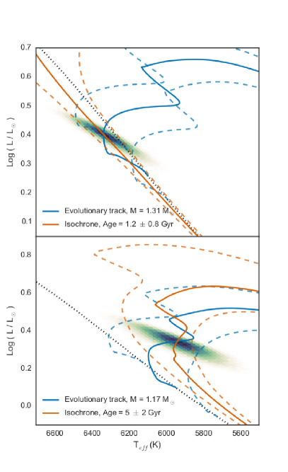
Figure 8: BAGEMASS stellar mass and age analysis of WASP-86 (upper panel) and WASP-102 (lower panel). The dotted black line is the ZAMS. The solid blue line is the mass evolutionary track, and the blue dashed tracks on either side are for the 1–$\sigma$ error of the mass. The solid orange line is the stellar age isochrone and the orange dashed lines represents the 1–$\sigma$ error. The density of MCMC samples is shown in the colour scale of the posterior distribution plotted.

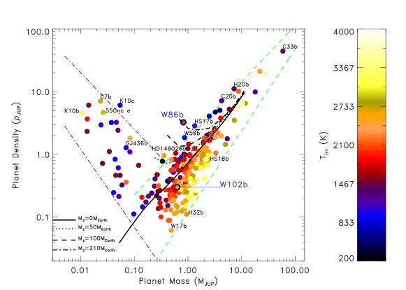
Figure 9: Planetary density versus mass and irradiation temperature (colours) for all planets with precisely derived masses and radii (better than 20%). We also plot boundaries in this plane (green–dashed and blue–dot-dashed lines) as derived in Bakos et al. (2015) but we estimate different values which are described in §5. In black, we show theoretical models of planetary interiors (Fortney et al. 2007; Baraffe et al. 2008) for different core masses: 0M_⊕ solid line, 50M_⊕ dotted line, 100M_⊕ dashed line, and 210M_⊕ dot-dashed lines. The latter is obtained by extrapolation from the models above. The loci of WASP-86b and WASP-102b are indicated in navy blue. WASP-86b is a clear outlier and is the most dense planet among planets with masses between that of Neptune and 2M_J, making it quite exceptional. Other planets are indicated by their name in full or with the following criteria: K for Kepler, H for HAT, HS for HAT-South, C for CoRoT and W for WASP.

4.3 Planetary physical properties

The planetary properties were determined using our thoroughly tested Markov-Chain Monte Carlo (MCMC) analysis, which we performed including all available WASP and follow-up photometry, together with SOPHIE and CORALIE radial velocity measurements (as appropriate for each system). A detailed description of the method is given in Collier Cameron et al. (2007) and Pollacco et al. (2008).

In our iterative fitting we used the following jump parameters: the epoch of mid transit $T_{0}$, the orbital period $P$, the fractional change of flux proportional to the ratio of stellar to planet surface areas $\Delta F=R_{\rm pl}^{2}/R_{\star}^{2}$, the transit duration $T_{14}$, the impact parameter $b$, the radial velocity semi-amplitude $K_{\rm 1}$, the stellar effective temperature $T_{\rm eff}$ and metallicity [Fe/H], the Lagrangian elements $\sqrt{e}\cos\omega$ and $\sqrt{e}\sin\omega$ (where $e$ is the eccentricity and $\omega$ the longitude of periastron), and the systemic offset velocity $\gamma$. For WASP-102 we fitted the two systemic velocities $\gamma_{\rm\tiny CORALIE}$ and $\gamma_{\rm\tiny SOPHIE}$ separately to allow for instrumental offsets between the two data sets. In the case of WASP-86 we also fitted for a long term trend in the radial velocities ($d\gamma/dt$). The sum of the $\chi^{2}$ for all input data curves with respect to the models was used as the goodness-of-fit statistic. For each planetary system four different sets of solutions were considered: with or without the main-sequence mass-radius constraint (MS constraint) and in the case of circular orbits or orbits with floating eccentricity.

An initial MCMC solution with a linear trend in the systemic velocity as a free parameter was explored for the two planetary systems. In the case of WASP-86 a linear trend to the RV data was found to be significant. When exploring solutions with non-circular orbits the Lucy & Sweeney F-test was performed Lucy & Sweeney (1971), and in both cases this returned a probability of 100% that the improvement in the fit produced by the best-fitting eccentricity could have arisen by chance if the orbit were in fact circular. For the treatment of the stellar limb-darkening, the models of Claret (2000, 2004) were used in the $r$-band, for WASP, SPM, NITES, LT and Euler photometry, and in the $z$-band for TRAPPIST and FTN photometry. At each MCMC chain step we look-up the limb-darkening coefficients from these tabulations using the value of $T_{\rm eff}$ for that step assuming $\log g$as derived in Table 5.

We calculate the mass $M_{\star}$, radius $R_{\star}$, density $\rho_{\star}$, and surface gravity $\log g$ of the host stars as well as $M_{\rm pl}$ , $R_{\rm pl}$ , $\rho_{\rm pl}$  and $\mbox{$\log g$}_{\rm{pl}}$  for the planets and their the equilibrium temperatures assuming a black-body ($T_{\rm pl,A=0}$) and efficient energy redistributed from the planet’s day-side to its night-side. We also calculate the transit ingress/egress times $T_{\rm 12}$/$T_{\rm 34}$, and the orbital semi-major axis $a$. All calculated values and their 1–$\sigma$ uncertainties are presented in Table 7. The corresponding best-fitting transit light curves are shown in Figures 3 and 4. The best-fitting RV curves are presented in Figure 5.

For both planets, circular orbits and no main-sequence constraint on the stellar mass and radius were selected. We find that imposing the MS constraint has little effect on the MCMC global solution in the case of WASP-86, while in the case of WASP-102 imposing the MS constraint was increasing the posterior probability values for the stellar temperature and metallicity beyond their 1–$\sigma$ spectral uncertainties as derived in our analysis in §4.1.

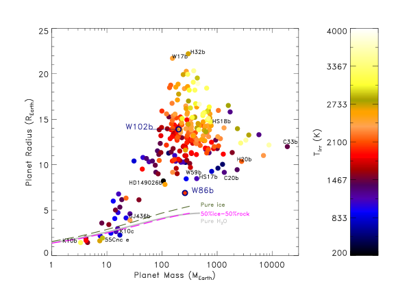
Figure 10: Planetary radius versus mass and irradiation temperature (colours) as in Figure 9. We also plot models of planet interior for three different compositions: pure ice (olive dashed line), 50% water – 50% rock (magenta dashed line) models from Fortney et al. (2007), and pure water (grey solid line) models are from Zeng & Sasselov 2013. The loci of WASP-86b and WASP-102b are indicated in blue circle and label. We note that WASP-86b is remarkably close to the right–bottom corner where planets are forbidden simply because they would be too massive for their host star to form (Mordasini et al. 2012). . Other planets are indicated by their name in full or with the following criteria: K for Kepler, H for HAT, HS for HAT-South, C for CoRoT and W for WASP. All planets had parameters derived to better than 20%.

Table 7: System Parameters of WASP-86 and WASP-102

	WASP-86	WASP-102
$P$	5.031555${}^{+0.000002}_{-0.000002}$	2.709813${}^{+0.000005}_{-0.000004}$	d
$T_{0}\leavevmode\nobreak\ ^{\dagger}$	7103.7527${}^{+0.0004}_{-0.0006}$	6510.5872$\pm$0.0002	d
$T_{\rm 14}\leavevmode\nobreak\ ^{\ddagger}$	0.1674${}^{+0.0015}_{-0.0010}$	0.1459$\pm$0.0005	d
$\Delta F=R_{\rm pl}^{2}/R_{\star}^{2}$	0.0025307$\pm$0.00008	0.00946$\pm$0.00010
$b$	0.027${}^{+0.036}_{-0.020}$	0.03${}^{+0.05}_{-0.02}$	$R_{\star}$
$i$	89.85${}^{+0.11}_{-0.20}$	89.73${}^{+0.19}_{-0.145}$	∘
$K_{\rm 1}$	0.084$\pm$0.005	0.082$\pm$0.006	km s-1
$\gamma$	-23.658${}^{+0.006}_{-0.005}$	-16.5453$\pm$0.0007	km s-1
$\gamma_{2}$	…	-16.4803$\pm$0.0002	km s-1
$d\gamma/dt$	0.0000823${}^{+0.0000089}_{-0.0000082}$	0. (fixed)	km s-1$d^{-1}$
$e$	0. (fixed)	0. (fixed)
$M_{\star}$	1.239$\pm$0.028	1.167$\pm$0.035	M⊙
$R_{\star}$	1.291${}^{+0.014}_{-0.013}$	1.331${}^{+0.013}_{-0.012}$	R⊙
$\log g_{\star}$	4.309$\pm$0.006	4.257$\pm 0.006$	cgs
$\rho_{\star}$	0.57$\pm$0.01	0.419${}^{+0.017}_{-0.009}$	$\rho_{\odot}$
$M_{\rm pl}$	0.821$\pm$0.056	0.624$\pm$0.045	MJ
$R_{\rm pl}$	0.632${}^{+0.014}_{-0.013}$	1.259$\pm 0.016$	RJ
$\log g_{\rm pl}$	3.67$\pm$0.03	2.95$\pm$0.03	cgs
$\rho_{\rm pl}$	3.24${}^{+0.31}_{-0.26}$	0.311${}^{+0.024}_{-0.022}$	$\rho_{\rm J}$
a	0.0617$\pm$0.0005	0.0401$\pm$0.0004	AU
$T_{\rm eq}$	1415$\pm$22	1705$\pm$32	K

^† BJD – 2 450 000.0
^‡ $T_{\rm 14}$: transit duration, time between 1^st and 4^th contact

5 Discussion

5.1 Comparative exoplanetology

WASP-86 is a young F7 star of about only 1 Gyr old. With a radius of $R_{\rm pl}$ = 0.632 $R_{\rm J}$ and a mass $M_{\rm pl}$ = 0.821 $M_{\rm J}$, WASP-86b has a density of $\rho_{\rm pl}$ =3.24 $\rho_{\rm J}$, and is thus the densest planet with mass in the range 0.05M_J (Neptune mass) $<M_{\rm pl}<$ 2 M_J. Only giant planets with masses larger than about 2$M_{\rm J}$ have larger densities, making WASP-86b exceptional in its mass range. Figure 9 shows the planetary density ($\rho_{\rm J}$) versus mass (M_J) and irradiation temperature as derived in Heng (2012), for all planets with precisely derived masses and radii (better than 20%). We show the loci of WASP-86b and WASP-102b in navy blue. The black curves are planet structure models from Fortney et al. (2007) with core masses of 0 (solid line), 50$M_{\oplus}$ (dotted line), 100$M_{\oplus}$ (dashed line), and 210$M_{\oplus}$ (dot-dashed line). Figure 9 also shows upper and lower boundaries in this plane following the functional form of Bakos et al. (2015). The values of the power law we obtain are however different from those derived in Bakos et al. (2015) and are as follows:

$$\rm{For}\leavevmode\nobreak\ M_{\rm pl}<0.4M_{\rm J}\,,\,\cases{\rho_{\rm pl}}<10^{-2.40}\times(M_{\rm pl}/M_{\rm J})^{-1.24}\\ \rho_{\rm pl}>10^{-0.50}\times(M_{\rm pl}/M_{\rm J})^{-0.90}\\ {}$$

$$\rm{For}\leavevmode\nobreak\ M_{\rm pl}>0.4M_{\rm J}\,,\,\cases{\rho_{\rm pl}}<1.8\times(M_{\rm pl}/M_{\rm J})^{0.90}\\ \rho_{\rm pl}>0.12\times(M_{\rm pl}/M_{\rm J})^{1.30}\\ {}$$

WASP-86b is a clear outlier. Similar objects with lower densities are HD 149026b (Sato et al. 2005), WASP-59b (Hébrard et al. 2013) and HATS-17b (Brahm et al. 2016).

5.2 Likely disc mass

With a stellar mass of $\sim$1.3 $M_{\odot}$ and an [Fe/H] = $+0.23$ dex, WASP-86 is predicted to possess a higher content of heavy elements, and thus possibly host additional massive planets (Mordasini et al. 2012). The maximal planetary mass and disc gas-mass are correlated because gas giant planets (in the core accretion scenario) accrete most of their mass in a regime where their accretion rate is proportional to the disc gas-mass (Guillot et al. 2006; Burrows et al. 2007; Miller & Fortney 2011). This correlation implies that the metallicity of the system determines the maximum mass a planet can grow up to in a given disc (Mordasini et al. 2012). The total amount of heavy elements (M_Z) available in the protoplanetary disc during planet formation is given by $\rm{M_{z}}=\rm{M_{Disc}}\,\,Z_{\odot}\,\,10^{[Fe/H]}$ (Mordasini et al. 2014; Baraffe et al. 2008), where Z_⊙ is 0.015. M_Disc is the maximum mass of a stable protoplanetary disc which is M${}_{\rm Disc}\lesssim 0.1\rm{M_{\star}}$ (Ida & Lin 2004; Mordasini et al. 2012). In the case of WASP-86 the maximum heavy element content present in the disc was:

$$\rm{M_{z}}=0.1\times 1.24M_{\odot}\times 0.015\leavevmode\nobreak\ 10^{+0.23}(3.3\leavevmode\nobreak\ 10^{5}\leavevmode\nobreak\ M_{\oplus}/M_{\odot})\simeq 10^{3}M_{\oplus}$$

According to models of planet formation and migration up to $\sim$ 30% of the heavy elements content of the protoplanetary disc can be accreted onto planets (Alibert et al. 2005, 2006; Mordasini et al. 2009, 2012; Dodson-Robinson et al. 2009). For WASP-86b the maximum mass of heavy elements available in the disc amounts to about 330M_⊕.

5.3 Heavy metal content

In order to match WASP-86b’s high density, an extrapolation from the theoretical models of Fortney et al. (2007) and Baraffe et al. (2008) predicts a planet composition of more than 80% heavy elements (either confined in a core or mixed in the envelope). If confined in a core, this value corresponds to a core mass of approximately 210$M_{\oplus}$ (Fortney et al. 2007) for a planet with mass $M_{\rm pl}\sim 260\leavevmode\nobreak\ M_{\oplus}$; Figure 9 shows theoretical models of the planetary interior from Fortney et al. (2007). WASP-86b’s heavy element enrichment is quite close to the above derived 30% upper limit of accretion efficiency. For models such as those of Baraffe et al. (2008) which consider the case of heavy elements mixed in the envelope (a more realistic model for gas giant interiors), the maximum difference in the planet radius is about 10-12% smaller compared to the radius estimated by Fortney et al. (2007). Thus a lower amount of heavy elements is needed to match the planet radius for the same mass. Using the models by Baraffe et al. (2008) we estimate a mass fraction of heavy elements of $\gtrsim$80% for WASP-86b. Planets with heavy element mass fractions of $>50\%$ are possible (Baraffe et al. 2008; Mordasini et al. 2009), and a massive core for WASP-86b can be expected given the high metallicity of its host star. However, the estimated value of a core mass of 210M_⊕implies very large accretion rates and substantial planet migration. Therefore, WASP-86b could have formed far out in the disc and consequently migrated most probably via Type II migration (Mordasini et al. 2009, 2012, 2014). This scenario could explain the circular orbit of WASP-86b (Dunhill 2015), as well as the growth of a very massive core given the larger available mass reservoir as the planet migrates within the disk (Mordasini et al. 2014).

5.4 Planetary envelopes

Giant planets are expected to form far out in the protoplanetary disc and then migrate inward. Massive cores can form at larger distances in the protoplanetary disc, but even if the material is available in the disc the planetesimal accretion rate must exceed the gas accretion rate which seems unlikely for massive cores. Additionally, WASP-86b seems to lack a massive hydrogen-helium envelope. To better understand the peculiarity of WASP-86b we show in Figure 10 the mass-radius parameter space for all planets as in Figure 9. WASP-86b is at the edge of the forbidden zone at the right-bottom corner of the diagram where planets can not be found simply because they would be too massive for their host star planetary disc to form. In Figure 10, we also plot, as reference, models of planetary interior composition for planets with pure ice and 50% water – 50% rock from Fortney et al. (2007); and pure water models from Zeng & Sasselov (2013). Any gas giant planet is expected to have a core mass of about 10-15 $M_{\oplus}$ (Alibert et al. 2005; Mordasini et al. 2009) under the core accretion scenario (although the exact value is still unclear Miller & Fortney 2011). Once this core mass is reached then ‘run-away’ gas accretion takes place, and indeed every planet with $M_{\rm pl}$$\geq 100M_{\oplus}$ has an envelope. Figure 10 shows that compared to other gas giants of the same mass WASP-86b has a much smaller H/He envelope.

5.5 Our formation scenarios

5.5.1 WASP-86b

To reconcile all the above mentioned characteristics of WASP-86b we propose a different formation scenario whereby the planet has formed and migrated inward and, after the disc dispersal, the planet has undergone a major impact with another body in the system. Numerical simulations show that major impacts of two super-Earth like planets, or the merger of more massive giant planets, can lead to complete coalescence of the two bodies (Liu et al. 2015). Moreover, Petrovich (2015) show that in unstable systems, planets at short semi-major axes ($<0.5$AU) are more likely to collide rather than have their orbits excited to high eccentricities and inclinations.

A similar scenario has been proposed to explain other compact planets such as HAT-P-2b (Baraffe et al. 2008), HD 149026b (Ikoma et al. 2006) and HATS-17b (Brahm et al. 2016). In such an event the original planet can be stripped of the majority if not all of its envelope (Ida & Lin 2004; Liu et al. 2015) which could possibly explain the lack of a large gaseous envelope for WASP-86b. Interestingly, given the young age of WASP-86 (about 1 Gyr), and its circular orbit, such a major impact might just have taken place in an event similar to the late heavy bombardment in the Solar system, which is thought to have happened $\sim$600Myr after formation (Pfalzner et al. 2015). Thus the WASP-86 system could provide a window into planet formation and dynamics at an age that was crucial for the development of our Solar system (Gomes et al. 2005). Observational signatures of giant impacts dissipate on timescales that are much too short to be observable in the WASP-86 system (Jackson et al. 2014), thus an abnormally high giant planet density might represent one of the only indirect ways in which we could deduce the existence of a giant impact. This hypothesis is also supported by recent models of planet formation via population synthesis (Mordasini et al. 2012, 2014) which show in their synthetic mass-radius relation that planets with densities as high as that of WASP-86b, and a heavy elements enrichment of 80%, have masses below 40M_⊕ and radii smaller than 5.2R_⊕.

Caveat for our scenario. It must be noted that in the case where the presence of the third body in the WASP-86 system is confirmed and is a low-mass stellar companion, its light could be diluting the transit light curve making the planet radius to appear smaller. We can however reject from our analysis of the spectra a high-mass star. High-angular resolution imaging, like Lucky Imaging we have applied for, will enable us to determine if such dilution exists and thus confirm the dense nature of the planet.

5.5.2 WASP-102b

At the opposite end of the spectrum from WASP-86b, WASP-102b is a sub-Jupiter gas giant planet with twice the mass of Saturn that shows a moderate radius anomaly as defined by Laughlin et al. (2011). With a metallicity of [Fe/H] = $+$0.09 dex, WASP-102b is not expected to possess a large core. However, with a radius of 1.259R_J, WASP-102b is $\sim$15% larger than predicted for a coreless model of a planet orbiting at 0.045 AU from the Sun for the age of 4.5 Gyr (Fortney et al. 2007; Baraffe et al. 2008). Figures 9 & 10 show the mass–density and mass–radius plots for all planets as described above. WASP-102b (highlighted in blue) belongs to the class of moderately irradiated systems showing larger than model–predicted radii. Figure 10 shows that the maximum extent of the radius anomaly is observed for planets with masses between $\sim$0.3 M_J ($\sim 100$ M_⊕, i.e. Saturn mass) and 0.7 M_J (223 M_⊕).

The planetary radius depends on multiple physical properties such as the age, the irradiation flux, the planet’s mass, the atmospheric composition, the presence of heavy elements in the envelope or in the core, the atmospheric circulation, and also on any source generating extra heating in the planetary interior. Because of WASP-102b’s short orbital period and circular orbit, the amount of irradiation received from its host star is probably the most important cause of WASP-102b’s large radius (assuming an age of 5 Gyrs). The planet equilibrium temperature, estimated assuming zero albedo and efficient energy redistribution between the planet’s day– and night–sides, is T_eq = 1705 $\pm$ 32 K which is close to the temperature threshold of 2000 K, below which Ohmic heating seems to be less important (Perna et al. 2012). Different possible mechanisms can play a significant role in determining WASP-102b’s radius anomaly, namely tidal heating due to unseen companions pumping up the eccentricity (Bodenheimer et al. 2001, 2003), kinetic heating due to the breaking of atmospheric waves (Guillot & Showman 2002), enhanced atmospheric opacity (Burrows et al. 2007), and semi-convection (Chabrier et al. 2007). All the above, however, can not explain the entirety of the observed radii (Fortney & Nettelmann 2010, Leconte et al. 2010). Because of their radius degeneracy close-in planets, in particular at sub-Jupiter masses (0.3 - 0.7M_J), represent a challenge for theoretical models reproducing their radii and thus the radius anomalies currently remains an unresolved problem in the field of exoplanets. More systems such as WASP-102b can help improve our understanding of planetary radii by means of the comparison among planets of similar mass and completely different ages and irradiation environments.

5.6 Tidal spin-up of WASP-102

A possible explanation for the discrepancy between the age of WASP-102 estimated via gyrochonology and that obtained using stellar evolutionary models (see §4.2) could be tidal interactions between the star and the planet. If the stellar rotation period is longer than the planetary orbital period, significant orbital angular momentum is transferred from the orbit of a planet to the rotation of the host star (“tidal spin-up”) via tides, yielding a star that is rotating faster than an isolated star of the same age.

Age estimation via gyrochonology assumes a natural rotational evolution for the star, free from any external influence. This is not always the case; in both binary star systems and hot Jupiter exoplanetary systems, tidal torques between bodies in close proximity can potentially overwhelm the natural spin-down that results from magnetic braking. If this is the case for WASP-102 then the stellar gyrochronological age will be underestimating its true age (Zahn 1975, 1977; Goodman & Lackner 2009; Ogilvie 2014; Damiani & Lanza 2015). Under this scenario, tidal heating would also partially explain the large radius of WASP-102b. However, WASP-102b would remain a larger than model-expected planet for its mass, orbital distance and age.

Higher stellar rotation rates (measured either directly, or by means of $v\sin i$) in systems with hot Jupiters have been proposed as indications of a tidal influence of exoplanets on their host star (Husnoo et al. 2012). Under the assumption that the star has been spun up by the presence of the planet, then from the increase in stellar rotation we would also expect an increase in stellar activity because rotation is a major driver of activity (Poppenhaeger & Wolk 2014). However, we do not detect any indication of stellar activity in our spectra (Ca II H&K) nor in the analysis of the WASP data.

Recent studies of the discrepancy between stellar ages estimated via gyrochronology and those estimated using stellar models highlight an existing bias towards older ages when using isochronal analysis owing to the uneven spacing of data in isochrones near the ZAMS (Brown 2014; Soderblom 2010; Barnes 2007; Saffe et al. 2005). Recently, Maxted et al. (2015b) explored this discrepancy for 28 exoplanet host stars and found strong evidence showing that, for half of the stars in their sample, gyrochronological ages of planet host stars are significantly lower than the isochronal ages. This is also the case for WASP-102b. Given WASP-102b’s short orbital period and relatively large mass, it is possible that tidal interactions have spun up the planet’s host star. However, given that Maxted et al. (2015b) show that the age discrepancy is not always good evidence for tidal interactions, more observational evidence would be necessary in order to confirm tidal spin-up of the star.

6 Conclusion

In this paper we have reported the discovery of two new gas giant planets, WASP-86b and WASP-102b, from the SuperWASP survey. New discoveries from ground-based transit surveys show that the currently known population of gas giant planets is by no means exhaustive. More peculiar systems such as WASP-86b and many others, including WASP-127b (Lam et al. 2016), HATS-18b (Penev et al. 2016), and EPIC212521166 b (Osborn et al. 2016), just to mention a few, continue to provide invaluable observable constraints for theoretical models of formation and evolution of planetary systems.