Ammonia and CO Outflow around 6.7 GHz Methanol Masers

Abstract

Single point observations are presented in NH₃ (1,1) and (2,2) inversion transitions using the Effelsberg 100 m telescope for a sample of 100 6.7 GHz methanol masers and mapping observations in the ¹²CO and ¹³CO $(1-0)$ transitions using the PMO Delingha 13.7 m telescope for 82 sample sources with detected ammonia. A further 62 sources were selected for either ¹²CO or ¹³CO line outflow identification, producing 45 outflow candidates, 29 using ¹²CO and 16 using ¹³CO data. Twenty-two of the outflow candidates were newly identified, and 23 had trigonometric parallax distances. Physical properties were derived from ammonia lines and CO outflow parameters calculated. Histograms and statistical correlations for ammonia, CO outflow parameters, and 6.7 GHz methanol maser luminosities are also presented. No significant correlation was found between ammonia and maser luminosity. However, weak correlations were found between outflow properties and maser luminosities, which may indicate that outflows are physically associated with 6.7 GHz masers.

1 Introduction

Massive stars ($>8$M_⊙) play a dominant role in shaping galactic structure and evolution. Although Shu et al. (1987) provided a detailed description on low mass star formation, massive star formation remains under debate. Zinnecker & Yorke (2007) summarized the massive star formation process into a four-phase evolutionary sequence, similar to low mass stars, and proposed that high mass star formation is not merely a scaled up version of low mass formation, but involves new and different physical processes. However, challenges in observing high mass star forming regions has hindered understanding, with massive stars being statistically rare, at large distances, evolving rapidly with short lived evolutionary phases, deeply buried in dense molecular envelopes, and usually interacting with nearby complex star forming compounds (Shepherd & Churchwell, 1996a; Zinnecker & Yorke, 2007).

Signposts to trace massive star formation regions are usually water, methanol, and hydroxyl masers. Class II methanol masers in the $5_{1}-6_{0}~{}\mathrm{A}^{+}$ transition (at 6668.5192 MHz) (Menten, 1991; Sobolev et al., 1997) are brightest after H₂O and are suggested to be only associated with massive star formation. The 6.7 GHz methanol masers appear before the UCH II region phase (hot core phase), and disappear as the UCH II region evolves (e.g. Codella & Moscadelli, 2000; Codella et al., 2004; van der Walt, 2005). The 6.7 GHz methanol maser pumping mechanism is considered to be radiative, requiring specific temperatures and column densities that are not expected in low mass young stellar objects (YSOs) (Cragg et al., 2005). Observations of low mass star forming regions have supported this non-detection (e.g. Minier et al. 2003, Bourke et al. 2005, Pandian et al. 2008, Green et al. 2012). Breen et al. (2013) also examined some masers associated with evolved stars and confirmed the 6.7 GHz methanol masers are exclusively associated with massive star forming regions.

Massive stars are considered to be initially born in giant molecular clouds (GMCs), so one might essentially want to know the physical conditions in the star forming regions. The inversion lines of ammonia, particularly the NH₃ (1,1), (2,2), and (3,3) lines, are excellent thermometers of the dense gas because they are collision excited and the molecules are not easily depleted onto dust grains (Ho & Townes, 1983; Mangum et al., 1992; Bergin & Langer, 1997). Therefore, key gas parameters, such as temperature, opacity, and column density can be estimated by measuring inversion line intensity. Physical property differences between weak and strong 6.7 GHz methanol masers have been discussed widely. Szymczak et al. (2000) suggested that IRAS colors vary with maser luminosity, but Pandian & Goldsmith (2007) did not confirm this difference. Wu et al. (2010) found physical properties differences derived from ammonia lines and 6.7 GHz methanol maser luminosity, but Pandian et al. (2012) later disproved these findings with a larger and less biased sample.

Molecular outflows are useful probes of star-forming activities in early phases. In the disk-jet model of low mass star formation, molecular outflows are a phenomenon of surrounding gas entrained by high-velocity jets or star winds. As the first CO outflow was discovered in Orion KL by Kwan & Scoville (1976), accumulated observations of high mass star formation regions show outflows are also common in massive star formation regions (e.g. Snell et al., 1990; Shepherd & Churchwell, 1996a; Ridge & Moore, 2001; Beuther et al., 2002; Wu et al., 2004; Xu et al., 2006; Arce et al., 2007; de Villiers et al., 2014; Maud et al., 2015), indicating a similar driven mechanism. Despite the similarity, whether there are differences between low and high mass star formation region outflows (Beuther et al., 2002; Wu et al., 2004; Zinnecker & Yorke, 2007) remain under debate.

Outflow properties are correlated with physical properties of the central source (Beuther et al., 2002; Wu et al., 2004; Zhang et al., 2005; de Villiers et al., 2014). Methanol masers are also tracers of massive star formation, which leads to the question of whether outflows associate with methanol masers. Minier et al. (2000, 2001, 2002) and Codella et al. (2004) found that H₂O and CH₃OH masers were closely associated with the evolutionary phase when outflows are present. de Villiers et al. (2014, 2015) analyzed CO $(J=3-2)$ line data in 54 6.7 GHz methanol maser sources and identified 44 resolvable methanol maser associated outflows (MMAOs). They also investigated relationships between outflow and maser properties, and suggested that the maser pumping source may be the outflow driver.

Whether the luminosity of a methanol maser indicates different physical conditions traced by ammonia remains to be verified. In this work, we expand the sample of methanol masers to check the conclusions of Pandian et al. (2012). Although research on massive outflows tends to focus on high resolution observations, it is still necessary to expand the number of known outflow candidates in massive star formation regions through single dish surveys. In this study, ammonia properties and outflow identification was investigated exclusively around 6.7 GHz methanol masers to verify and investigate potential relationships. Some of the 6.7 GHz maser samples have accurate parallax distances, which can provide more reliable physical properties. Previous single dish surveys of molecular outflows in massive star formation regions have focused on molecular transitions such as CO $(2-1)$ and $(3-2)$. The present survey searched for ¹²CO $(1-0)$ and ¹³CO $(1-0)$ outflows around 6.7 GHz methanol masers using the PMO 13.7 m telescope.

Section 2 describes the sample, observations, and data reduction. Data analysis and derivation of physical properties are presented in Section 3. Outflow detection frequency, and relationships among ammonia, CO outflow, and maser properties are discussed in Section 4. Section 5 summarizes and presents the main conclusions.

2 Observations and Data Reduction

2.1 Sample selection

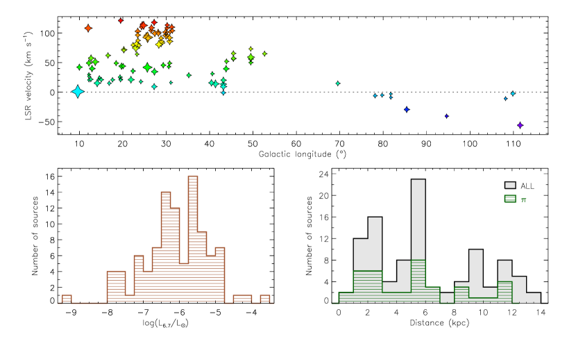
Figure 1: Top: Sample locations. Filled stars show the maser position. Symbol size represents maser luminosity. Bottom left: Methanol maser luminosities (6.7 GHz). Bottom right: Sample distances, $\pi$ represents parallax distances.

A sample of 100 sources with single point ammonia observations were selected from Caswell (2009) and Xu et al. (2009) with decl. $>-20^{\circ}$ and position accuracy better than 1^′′. he positions of these sources were determined by interferometer observations. Some sources have accurate trigonometric parallax distances calculated by the Bar and Spiral Structure Legacy (BeSSeL) survey and Japanese VLBI Exploration of Radio astronomy (VERA) (see Reid et al. 2009a and their serial papers; Reid et al. 2014). Distances of the remaining sources were determined kinematically from their observed radial velocities by applying model A5 in Reid et al. (2014) with a FORTRAN script by Reid et al. (2009b). Near or far distance ambiguities are either resolved using HI self-absorption or referring to allocations in the literature (Green & McClure-Griffiths, 2011; Dunham et al., 2011; Schlingman et al., 2011). If a source could not be resolved using HI self-absorption and have no previous allocations in the literature, we then take the near distance for it. The number of such sources is less than 10% of the sample.

Table 1 shows the chosen source maser properties, and their galactic locations are shown in the top panel of Fig. 1, with their distance distribution in the bottom-right panel. The sample covers a relatively wide range of maser luminosities (calculated from peak flux density, assuming isotropic emission and a typical line width to be 0.25 km s^-1) from $8.75\times 10^{-10}$ to $2.36\times 10^{-4}$ L_⊙, as shown in the bottom left panel of Fig. 1. Sample sources overlaid on an artist’s conception of the Milky Way galaxy seen from far Galactic North (R. Hurt: NASA/JPL-Caltech/SSC) is shown in Fig. 2.

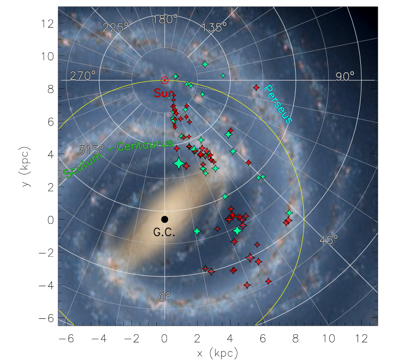
Figure 2: Sample sources overlaid on Milky Way skeleton by R. Hurt. Filled stars represent sources with accurate parallax distances, open stars with red $+$ have kinematic distances.

2.2 Ammonia observations

Single point observations of the sample in ammonia inversion transitions NH₃(1,1) NH₃(2,2) were performed during March 2011 and May 2012 using the Effelsberg 100 m telescope. A dual channel cooled K-band HEMT receiver with two polarizations (LCP/RCP) was used as the frontend, and a fast Fourier transform spectrometer (FFTS) as the backend. The FFTS was set to Narrow-Band-IF mode with a bandwidth of 100 MHz at 24 GHz. It had 32,768 channels in each IF inputs, allowing simultaneous observation of the two lines, with velocity channel separation 0.038  km s^-1. The observations were made in frequency switched mode with frequency throw 7.5 MHz. Integration times ranged from 4–13 minutes depending on the system temperature, which varied from 60–90 K. Pointing accuracy was found to be better than 10^′′. Flux calibration was accurate to 10%, estimated by observing the standard source W3(OH). Flux density was converted to main beam brightness temperature ($T_{\mathrm{mb}}$), assuming a conversion factor of 1.36 K Jy^-1 (using Equation 8.20 in Wilson, Rohlfs and Hüttemeister, 2009). Half power beam width (HPBW) of the telescope at the observed frequency was approximately 40^′′. All spectra were smoothed to a velocity channel separation of 0.32 km s^-1. NH₃ data were reduced using the CLASS package of the GILDAS software distribution developed by IRAM.

2.3 CO observations

¹²CO, ¹³CO  and C¹⁸O $J=1-0$ data were obtained using the Purple Mountain Observatory (PMO) Delingha 13.7 m millimeter telescope in May and June 2014, and supplementary observations were performed in June 2015. A $10^{\prime}\times 10^{\prime}$ area was mapped around each sample source, using a 3$\times$3 multi-beam superconducting spectroscopic array receiver (SSAR) with a two sideband superconductor insulator superconductor (SIS) mixer as the frontend (Shan et al., 2012). The receiver enabled the three CO lines to be simultaneously observed, ¹²CO line in the upper sideband (USB), and ¹³CO and C¹⁸O in the lower sideband (LSB). The backend employed a high definition FFTS with 1 GHz bandwidth. The spectrometer provided 16,384 channels, corresponding to velocity channel separation 0.16 km s^-1 for ¹²CO and 0.17 km s^-1 for ¹³CO and C¹⁸O. Typical system temperatures were approximately 210 K for USB and 130 K for LSB measurements. Pointing accuracy and tracking errors were better than 5^′′. HPBW at 115.271 GHz was approximately 52^′′. Mapping observations were made using on the fly (OTF) mode with a scan speed of 50^′′ s^-1 and a step size of 15^′′ along Galactic longitude or latitude. Standard sources were observed at intervals to estimate main beam efficiencies ($\eta_{\mathrm{mb}}$), which were calibrated by incorporating an elevation based antenna gain curve. Mean $\eta_{\mathrm{mb}}$ were 48% for USB and 52% for LSB, with variations dominated by elevations. The antenna temperatures were converted to main beam temperatures using $\eta_{\mathrm{mb}}$ above. Mean rms noise level of the spectra was approximately 0.5 K for ¹²CO and 0.3 K for ¹³CO and C¹⁸O after subtracting the linear baseline fit. Raw data were processed using pipeline scripts written in CLASS and GREG software packages. Spectral data were then meshed into cubes with grid spacing 30^′′. All data were saved as astronomical FITS files for subsequent analysis.

3 Data Analysis and Results

3.1 Ammonia line parameters

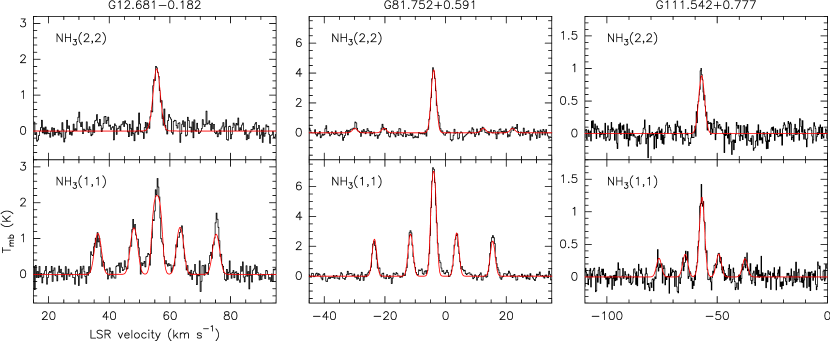
Figure 3: Three sample source NH₃ spectra with fitting lines for illustration. The NH3(1,1) method was used in CLASS to estimate opacities. The GAUSS method was employed to calculate FWHM for lines with weak satellite components.

Ammonia inversion transitions were observed to estimate the dense gas temperatures around the methanol maser site. A total of 82 sources show NH₃(1,1) and 73 NH₃(2,2) at the 3$\sigma$ level, 0.53 K. Fitting method NH3(1,1) was chosen for CLASS to model NH₃(1,1) lines incorporating hyperfine structure as well as deriving opacities, with the assumptions of Gaussian velocity distribution and equal excitation temperature. For NH₃(2,2) spectra, which usually show weak hyperfine components, the main component was fitted using the GAUSS method. Relevant fitting parameters and uncertainties, such as radial velocities with respect to the local standard of rest, brightness temperatures, line widths, and optical depths, are shown in Table 2. Figure 3 shows processed NH₃(1,1) and NH₃(2,2) spectra for three characteristic sample sources.

3.2 Ammonia line properties

Physical parameters of the dense environments around maser sites were derived from NH₃(1,1) and NH₃(2,2) transitions, providing excitation, kinetic, and rotational temperatures, as well as column density. The methods are described in appendix A, and the derived physical parameters are shown in Table 3.

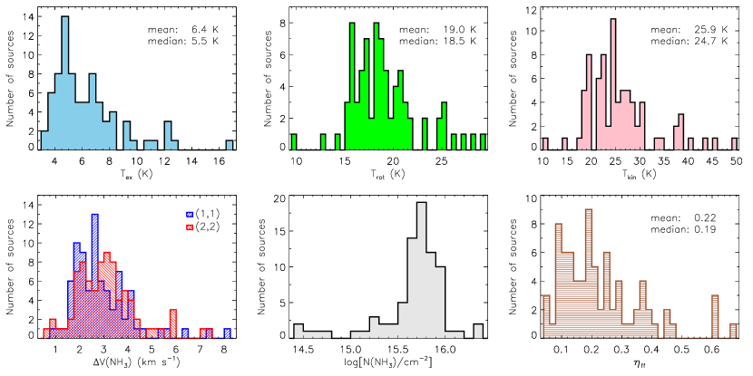
Figure 4: NH₃ line properties. Top three panels (left to right): excitation temperature, rotational temperature, and kinetic temperature. Bottom three panels (left to right): FWHM, NH₃ column density, and filling factor.

Figure 4 shows the statistics of observed and physical properties for NH₃ detect samples. The left top panel shows the excitation temperature, $T_{\mathrm{ex}}$, which ranges approximately 3.0–13.0 K, with mean and median 6.4 K and 5.5 K, respectively. These are lower than those of the low luminosity 6.7 GHz methanol maser sites in Wu et al. (2010), similar to those of the high luminosity 6.7 GHz methanol masers in Wu et al. (2010), but slightly higher than those studied by Pandian et al. (2012). These low values are most likely due to the small beam filling factor, $\eta_{\mathrm{ff}}$. If $T_{\mathrm{ex}}$ = $T_{\mathrm{rot}}$, then the typical beam filling factor turns = 0.19, significantly larger than 0.07, derived by Pandian et al. (2012).

The top middle panel of Figure 4 shows the sample rotational temperatures, which have a mean and median of 19.0 K and 18.5 K, respectively, slightly lower than those of Wu et al. (2010). Mean and median kinetic temperatures are 25.9 K and 24.7 K, similar to Pandian et al. (2012) and lower than Wu et al. (2010). The left bottom panel of Fig. 4 shows NH₃(1,1) and NH₃(2,2) FWHM for main component emission, with typical values 2.7 and 3.0 km s^-1, respectively. The line widths are comparable with Wu et al. (2010) and Pandian et al. (2012). And the ratio of the typical NH₃(2,2) to NH₃(1,1) line width is 1.1. Typical NH₃ column density of the sample masers was ${5.4\times 10^{15}}$ cm^-2, similar to Pandian et al. (2012).

3.3 CO outflow identification

Line profiles of ¹²CO$(1-0)$ and ¹³CO$(1-0)$ spectra at maser sites of the 82 sources with NH₃ detection were examined, and 62 were considered to be suitable for outflow identification. The selection criterion was that either ¹²CO or ¹³CO line wings should not be contaminated by velocity components along the line of sight that are not associated with 6.7 GHz maser emission. Both ¹²CO and ¹³CO spectra were used for outflow identification. Outflow wings are expected to be most obvious in ¹²CO$(1-0)$ due to its large abundance, but ¹²CO$(1-0)$ is often contaminated by extra components, while for ¹³CO$(1-0)$, which has a lower abundance than ¹²CO$(1-0)$, can be used in those cases where the wings of ¹²CO$(1-0)$ have contamination.

The following procedure was used to identify outflow candidates, with an example case, G85.410+0.003, shown in Figure 5.

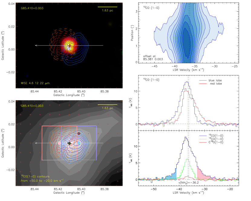
Figure 5: Sample outflow identification for the G85.410+0.003 methanol maser. The bottom left panel shows the outflow contours overlaid on integrated intensity of ¹²CO depicted as filled contours, which has LSR velocity range of -50 – -20 km s^-1 with contours from 10 K km s^-1 at step 12 K km s^-1. Brown crosses indicate CO data pixels. The maser position is marked with a brown filled star, and the yellow scale line in each panel is 1 arcmin. CO emission peaks are marked on the bottom left panel with dark blue and green circles around $\times$ and dark red circles around $+$ for ¹²CO, ¹³CO  and C¹⁸O, respectively. Then the lines shown in the bottom right panel are feature spectra extracted from the position of peak emission in the CO map. Red dashed vertical line is peak ¹³CO velocity, and black dashed vertical line is NH₃ velocity for comparison. Color filled areas under the line are the selected line wings. Integrating along the outflow wing ranges, we obtain the outflow lobes, which are illustrated as the blue and red contours within the blue and red boxes in the bottom left panel. The outflow contours start from 3.92 and 4.21 K km s^-1 with step 0.78 and 1.12 K km s^-1  respectively, to highlight prominent features. The spectra at the two lobe peaks are shown in the middle right panel. Blue and red lobe peak positions are marked in the bottom left panel with filled sky blue and pink circles, respectively. A position-velocity (P-V) slice diagram along the white arrow in the bottom left panel is shown in the top right panel. And finally a WISE 4.6, 12 and 22 $\mu$m false color image overlaid by outflow contours is shown in the top left panel.

Find peaks and extract feature spectra. The CO emission peak emission positions were located on the integrated intensity images, as shown in the bottom left panel of Figure 5. Although the ¹²CO and ¹³CO peak positions for G85.410+0.003 coincide with each other, the C¹⁸O peak is offset one pixel ($\sim 1.1$ pc), probably due to noise ambiguity and grid seperation. Generally, the ¹²CO, ¹³CO and C¹⁸O peaks do not coincide with each other and the maser point. Some peaks have offsets of one to two pixel spacing ($\sim 30^{\prime\prime}$). When sometimes the ¹²CO, ¹³CO and C¹⁸O peaks are all different from each other, then the position of either ¹²CO or ¹³CO peak that closer to the maser point was chosen to extract feature spectra. Spectra were then extracted from data cubes at the chosen peak position, providing feature lines for outflow identification (bottom right panel of Figure 5). To identify high velocity outflow components, the extracted spectra were smoothed to velocity resolution of 0.5–1.0 km s^-1 to reduce noise in an individual channel. The core velocities ($v_{\mathrm{peak}}$) were obtained at the line intensity peak for either ¹³CO or C¹⁸O  corresponding to the nearest maser and NH₃ peak velocity. Peak ¹³CO velocity was chosen when C¹⁸O emission was weak.

Outflow wings. Outflow wing ranges ($\Delta V_{\mathrm{b/r}}$) were determined by line diagnosis. Outflow wing is the component left after subtracting the Gaussian core profile. Since ¹³CO and C¹⁸O trace the denser core gas around YSOs, wing ranges were determined by comparison with different lines (Lada, 1985). For a typical ¹²CO line, blue and red wing velocity ranges were determined by ¹²CO velocity extent, where the ¹³CO line has no emission (e.g. the filled area of the line in the bottom right panel of Figure 5). ¹³CO emission was treated as the inner core component. Note that wing ranges were also manually adjusted according to the position velocity (P-V) diagram in the top right panel of Figure 5, which is described in the next procedure. The P-V diagram was included in Figure 5 to illustrate the velocity structure along the slice crossing outflow lobes. ¹³CO line wings were obtained similarly, but compared with C¹⁸O lines. ¹²CO wings are generally high velocity outer wings, while ¹³CO wings indicate inner wings, as discussed in Lada (1985).

Outflow contours and P-V diagrams. Outflow image was obtained by integrating the intensity along the wing velocity range (e.g. the top left and bottom left panels of Figure 5). Integrated contours were presented to highlight prominent features, starting mostly from 40% to 70% of the peak integrated intensities. The contours were then checked by naked eyes if they can be regarded as an outflow lobe. A blue or red box was added to restrict the boundary of a lobe (e.g. the blue and red boxes on the bottom left panel in Figure 5). Lobe area ($A_{\mathrm{b/r}}$) was calculated based on contours. Peak positions of lobes were located on the outflow contours (e.g. the blue and red filled circle on the bottom left panel in Figure 5)), and the spectra at lobe peaks were extracted for comparison (e.g. the middle right panel of Figure 5). Lobe length ($l_{\mathrm{b/r}}$) was then measured generally from the maser postion to the furthest radial distance along the line that connects the positions of two lobe peaks or one lobe peak to the central maser position (e.g. the white arrow shown in the bottom left panel of Figure 5). If outflow lobe peaks and maser point appeared to be on top of each other, the lobe length was then measured along the major axis. A P-V slice image (e.g. the P-V image on the top right panel in Figure 5) was also extracted along the line. For a typical outflow, the P-V diagram should show velocity bulges comparing non-outflow positions, and these velocity bulges were regarded as an evidence of outflow.

Comparisons with WISE false-color images. To uncover potential driving sources of the outflows, we used the high sensitivity mid-infrared images taken by the Wide-field Infrared Survey Explorer (WISE) (Wright et al., 2010). WISE maps the entire sky in four infrared bands W1, W2, W3, and W4 centered at 3.4, 4.6, 12, and 22 $\mu m$. A RGB false color image of WISE data at 4.6, 12, and 22 $\mu m$ overlaid with outflow contours was plotted for comparison. For instance, the infrared emission relating to the maser site can be clearly resolved in the top left panel of Figure 5. Most masers have a corresponding WISE detection at the same position. However, a few masers are difficult to cross identify the WISE detection, but some seem to have offsetting WISE sources. As de Villiers et al. (2014) stated, since there exist different hypotheses for the 6.7 GHz maser formation (they are either embedded in circumstellar regions around protostars or just in outflows). It is thus likely that some masers could be offset, while for a few other cases where the offset is too far, they probably do not have detectable WISE emission due to infrared extinction.

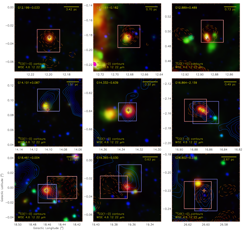
Figure 6: Newly identified outflows. Outflow contour lower limits and steps (within the boxes) are presented to highlight prominent features. Contours are overlaid on corresponding WISE false color images. ¹²CO and ¹³CO lines selected for outflow identification are labelled in the bottom left corner of each image. Symbols within each panel are the same as Figure 5.

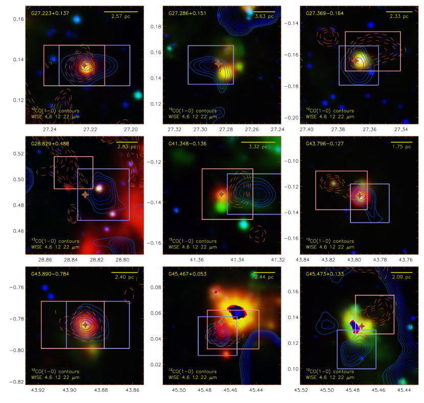
Figure 6: Continued.

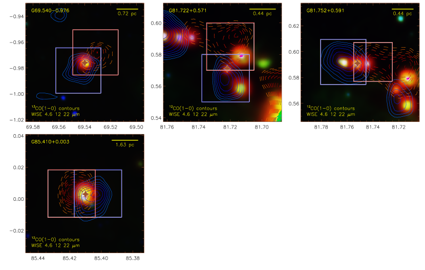
Figure 6: Continued.

Forty-five sources were identified to have significant CO outflow features from the 62 candidates with either ¹²CO or ¹³CO line wing. The detection frequency is 73%. Among these, 22 were newly identified, 29 were diagnosed with ¹²CO line wings and 16 with ¹³CO line wings. Detailed discussion regarding outflow detection frequency is presented in Section 4.1. The parameters for calculating outflow physical properties are shown in Table 4, and the 22 newly identified outflows are overlaid on corresponding WISE false color images in Figure 6.

3.4 CO outflow physical properties

Physical properties such as mass, energy, and momentum flux, must be estimated to allow outflow investigation. The estimates depend on estimates of optical depth, excitation temperature, and filling factor of the emitting gas, which provide column density as a function of velocity. The calculations are described in appendix B. Among the 45 outflow candidates, 23 have trigonometric parallax distances.

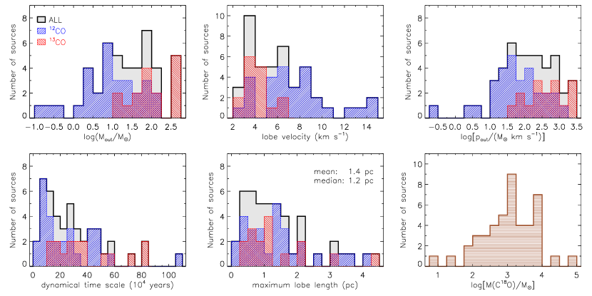
Figure 9: CO outflow properties without inclination correction. ¹²CO and ¹³CO outflow properties are distinguished for comparison. Top three panels: outflow mass, average lobe velocity, and momentum, respectively. Bottom three panels: dynamical time scale and maximum lobe size, respectively, of outflows and C¹⁸O cloud core masses.

The derived outflow physical properties are shown in Table 5. However, it is difficult to determine the outflows’ parameters precisely due to inclination, opacity and blending (Arce & Goodman, 2001). Since ¹³CO outflows are generally low velocity gas blended with ambient clouds, outflow mass may be overestimated. Inclination is also difficult to determine but has non-negligible effect on calculating outflow properties. Thus, statistically typical values were chosen for comparison with other works. Assuming a random distribution of inclination, the mean inclination was 57.3^∘ (Bontemps et al., 1996). This implies lobe velocity should be scaled up by a factor of 1.9, while dynamical age should be reduced by a factor of 0.6.

Outflow properties are shown in Figure 9, with typical ¹²CO and ¹³CO outflow masses 8 and 100 M_⊙, respectively. The mass difference arises from different estimation methods and distances. For ¹²CO, since the wing range does not show ¹³CO emission, the line wings were assumed to be optically thin, leading to a lower limit mass estimation. The mean and median mass of C¹⁸O cloud cores are both $1.3\times 10^{3}$ M_⊙. After inclination correction, the average lobe velocities of the sample outflows are typically 13 km s^-1 and 7.5 km s^-1 for ¹²CO and ¹³CO, respectively, because ¹²CO line widths are generally wider than ¹³CO and ¹²CO/¹³CO velocity ratio is approximately 2 (e.g. Cabrit et al., 1988; Shepherd & Churchwell, 1996b; Narayanan et al., 2012). In contrast to de Villiers et al. (2014), the wing velocities were not scaled for ¹³CO outflows.

Momentum is shown in the top right panel of Figure 9. Typical values corrected for inclination are 95 and 750 M_⊙ km s^-1 for ¹²CO and ¹³CO outflows, respectively. The mean maximum lobe length is 1.4 pc, incorporating the spatial resolution of the telescope and distance values. Outflow lobe sizes lower than the beam size limit ($\sim 55^{\prime\prime}$) were not able to be resolved. For the dynamical time scale presented in the bottom-left panel, typical values corrected for inclination are $1.1\times 10^{5}$ and $2.0\times 10^{5}$ years for ¹²CO and ¹³CO outflows, respectively. Such large values are an overestimation from the method described in Equation (B9). Since the $t_{\mathrm{d}}=l/v$ method can overestimate the flow age, Downes & Cabrit (2007) suggest a more accurate representation using $t_{\mathrm{d}}=1/3~{}l_{\mathrm{lobe}}/\langle v\rangle$, which provides typical dynamical timescales $3.8\times 10^{4}$ and $6.7\times 10^{4}$ years for ¹²CO and ¹³CO  respectively.

4 Discussion

A statistical analysis of the physical properties of the 6.7 GHz methanol masers is performed to investigate the underlying physics. There are several caveats regarding the results and correlations.

• Sample selection. The sources in the Galactic range of $0^{\circ}<l<20^{\circ}$ generally have multiple cloud components and distance ambiguities, adding uncertainty.

• The chosen sample set did not include all the masers in Caswell (2009) and Xu et al. (2009) with declination greater than $-20^{\circ}$ due to limited observation time. A more uniform sample with more sources is required to increase the reliability of the conclusions.

• The limited resolution and sensitivity of CO observations have large effects on determining outflow parameters.

Of the 45 identified outflow candidates, 23 have trigonometric parallax distances, and are treated separately in the statistical analysis. However, the statistical correlations will assist better understanding of massive star formation processes.

4.1 Outflow detection frequency

The chosen samples were all 6.7 GHz methanol masers, which are exclusively associated with massive star formation. The outflow detection frequency for the methanol masers was 73%. Of the 45 identified outflows, 29 have resolvable bipolar lobes. Those with one single resolvable lobe may be explained by their complicated environment. This detection rate only provides for a statistical valid result for CO observations using the PMO DLH 13.7 m telescope. Some sources without identified outflow, e.g. G29.956-0.016, could be identified outflows with higher spatial resolution or better intensity at higher transitions of CO (de Villiers et al., 2014). The high detection rate in previous outflow studies from massive YSOs shows that molecular outflows are a common phenomenon of massive star formation. Particularly when associating outflow with 6.7 GHz masers, the detection rate increases up to one hundred percent (de Villiers et al., 2014).

4.2 Outflow properties and source luminosity

Maud et al. (2015) selected a distance limited sample of 99 RMS MYSOs and identified 85 outflows. They showed that all outflow parameters scale with source luminosity and proposed two interpretations on the scaling relationships. One view was that the outflows are driven by the massive protostellar cores in an embedded cluster, supporting a scaled up version of the outflow driving mechanism verified for low mass stars. An alternative interpretation was that the relationships are observational effects, since outflow parameters are determined mostly by the entrained mass originating from the core, which allows for different star formation processes.

The correlations of outflow properties and source luminosity were checked across the chosen sample. IRAS luminosities were used, since IRAS point catalog provides relatively reliable flux densities at 12, 25, 60, and 100 $\mu$m. Zhang et al. (2005) examined the relationships between outflow mass rate and mechanical force against IRAS far-infrared luminosity, and found no significant correlations. Outflow properties and IRAS infrared luminosity are shown in Figure 10.

Tight correlations were found between outflow masses and infrared luminosity, with Pearson correlation coefficients $r=0.85$ and $r=0.74$ for ¹²CO and ¹³CO outflows, respectively. Since half of the outflow candidates have trigonometric parallax distances, these sources were fitted separately, with correlation coefficient $r=0.90$ for ¹²CO outflows (the number of ¹³CO outflows was too small to fit separately).

The mass outflow rate is also related to infrared luminosity, with $r=0.84$ and $r=0.52$ for ¹²CO and ¹³CO outflows, respectively. Again, when fitting ¹²CO outflows with parallax distances, the correlation coefficient increased to $r=0.88$, although this is partly due to the reduction of the number of sources. The correlation coefficient for outflow mechanical luminosity and infrared luminosity was 0.65. While Zhang et al. (2005) found no apparent correlation between luminosity, mass outflow rate and mechanical force, for the current sample, these outflow properties scale with IRAS infrared luminosity.

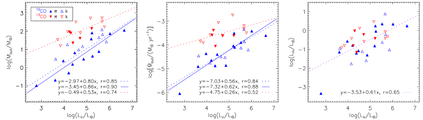
Figure 10: CO outflow properties and IRAS infrared luminosity. Left panel: Outflow masses as functions of infrared luminosity. Blue and red solid lines are linear fittings for sources with parallax distances. Blue and red dashed lines are the fitted ¹²CO and ¹³CO outflows, respectively. $\pi$ and k represent source distances calculated using parallax and kinematics, respectively. Middle panel: As the left panel, but for outflow mass rate and infrared luminosity. Right panel: Mechanical luminosity of outflow as a function of infrared luminosity. Purple dashed line shows the fitted outflow.

4.3 Ammonia line and outflow properties

As discussed in Section 3.4, the typical dynamical timescale for 6.7 GHz methanol maser associated outflows approaches $10^{5}$ years, through to the development of UCH II regions (Wood & Churchwell, 1989). The masers signpost a period of massive star formation before the UCH II phase (van der Walt, 2005), while molecular outflows are also a phenomenon in the early phases. Codella et al. (2004) provided a version of the evolutionary sequence in the hot core phase, and proposed: maser emission occurs before outflow; outflow appears and becomes detectable while maser emission is still present; maser emission disappears while outflow remains until the UCH II region is formed. de Villiers et al. (2015) amended the sequence and proposed that outflow appears and develops before maser emission. Maser emission appears when the in-fall process heats the dust grains and incubates certain conditions that can pump the methanol maser. Unfortunately, the dynamical timescales estimated by outflow surveys using single dish telescopes are too approximate to resolve the above evolutionary sequence. As noted in Maud et al. (2015), interferometric observations are required to resolve this issue. However, since outflow phase encompasses the methanol maser phase and the dynamical timescale can be derived through the outflow, physical conditions and dynamical properties around maser sites can be checked for evolutionary trends.

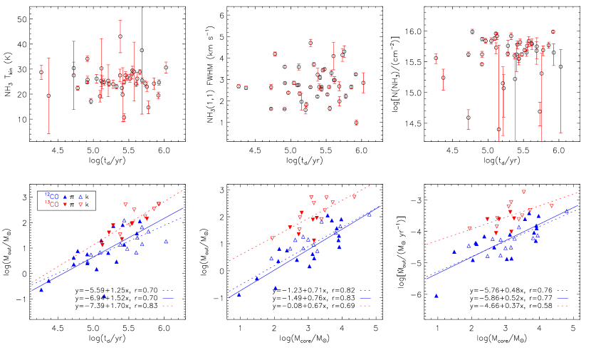
Figure 11: NH₃ and CO outflow properties. Top three panels: NH₃ kinematic temperatures, line widths, and NH₃ column densities, respectively, as functions of outflow dynamical timescales. Bottom left panel: Plot of outflow mass as a function of dynamical timescale. Bottom middle and right panels: outflow mass and outflow mass rate, respectively, as functions of core mass derived from C¹⁸O emission. Blue and red dashed lines are linear fits for ¹²CO and ¹³CO outflows, respectively. Blue solid lines are linear fits for ¹²CO sources with accurate parallax distances.

The top three panels in Figure 11 show the relations of NH₃ kinematic temperatures, line widths, and NH₃ column densities as functions of dynamical time. No significant correlations are present, which implies a lack of evolutionary trends.

The plot of outflow mass as a function of dynamical time, bottom left panel of Figure 11, shows significant correlations, with outflow mass increasing with dynamical timescale, correlation coefficients 0.70 and 0.83 for ¹²CO and ¹³CO outflows, respectively. Since both outflow mass and dynamical timescale relate to distance, such correlations can be expected. However, de Villiers et al. (2014) failed to find this correlation, and argued that their range of dynamical times was probably too small. Uncertainties in determining outflow properties may also mask the correlations.

Many other works have checked the relationships of outflow masses and core or clump masses (e.g. Beuther et al., 2002; de Villiers et al., 2014; Maud et al., 2015). The bottom middle panel in Figure 11 shows the relation of outflow mass and the source C¹⁸O core mass, with correlation coefficients 0.82 and $0.69$ for ¹²CO and ¹³CO outflows, respectively. The bottom right panel of Figure 11 shows the correlation of mass outflow rate and core mass, $r=0.76$, for ¹²CO outflows. These correlations agree with de Villiers et al. (2014), and are similar to those discussed in Maud et al. (2015). However, it is difficult to resolve whether the outflows arise from individual stars or multiple protostellar cores.

4.4 Physical properties and maser luminosity

Many previous surveys of 6.7 GHz methanol maser sources have investigated the correlation of maser luminosity and clump properties (e.g. Urquhart et al., 2013; Sun et al., 2014). Though more massive protostars usually have larger maser luminosities, the difference of physical conditions between the high and low luminosity masers remains undistinguishable. Wu et al. (2010) checked ammonia properties between high and low luminosity 6.7 GHz methanol masers. Although several differences were found, uncertainties due to lack of sample sources weakened the results. Pandian et al. (2012) expanded to a sample of 77 masers with single point ammonia observations. Aside from a weak correlation between maser luminosity and line width, no significant correlations were observed between the physical properties and maser luminosity.

The current sample was also examined for such correlations. The left panel of Figure 12 shows NH₃ column density and maser luminosity, with weak correlation, $r=0.23$, ignoring sources with large uncertainties. The sharp increase in NH₃ column density at higher maser luminosities, found in Wu et al. (2010), is not evident in the current sample set. NH₃ kinematic temperature and line width are shown in the middle and right panels, respectively, of Figure 12, with no significant correlations to maser luminosity, confirming Pandian et al. (2012).

Thus, NH₃ parameters have no evolutionary sequences in the hot phase (Section 4.3), and ammonia properties are independent of the environment around the maser sites.

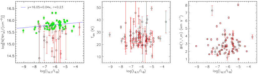
Figure 12: Left panel: 6.7 GHz maser luminosity and NH₃ column density. Green filled circles are sources with err$(\log[N(\mathrm{NH}_{3})/(\mathrm{cm}^{-2})])<0.1$. Blue line is the fitted green circles. Middle panel: 6.7 GHz maser luminosity and NH₃ kinematic temperature. Right panel: 6.7 GHz maser luminosity and NH₃$(1,1,m)$ FWHM line width.

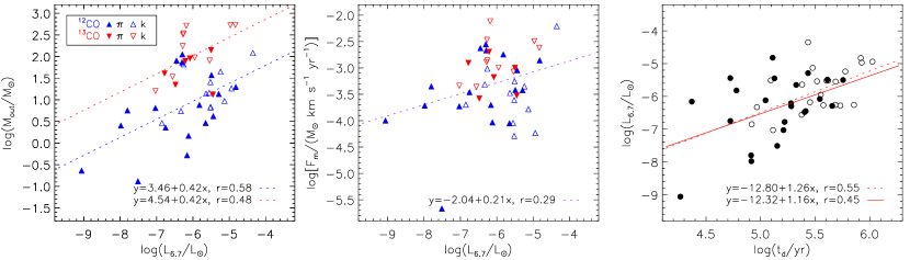
Figure 13: Left panel: 6.7 GHz maser luminosity and ¹²CO or ¹³CO outflow mass. Filled triangles represent sources with accurate parallax distances. Blue and red dashed lines are linear fits for ¹²CO and ¹³CO outflows, respectively. Middle panel: 6.7 GHz maser luminosity and outflow mechanical force. Purple dashed line is the linear fit. Right panel: 6.7 GHz maser luminosity and outflow dynamical time scale. Solid line is the linear fit for sources with parallax distances (filled circles), dashed line is the fit for all sources.

CO outflow properties were investigated for variance with maser luminosity. The left panel in Figure 13 shows that both ¹²CO and ¹³CO outflow masses rise with the maser luminosity, $r=0.58$ and 0.48, respectively, which is consistent with de Villiers et al. (2015). There is also a weak correlation, shown in the middle panel of Figure 13, between outflow mechanical force and maser luminosity. As discussed in Section 4.3, outflow driving source may be the pumping mechanism for the 6.7 GHz methanol maser, so a more powerful source driving more massive outflows may pump more maser emission. The right panel shows the evolutionary sequence of the maser luminosity, displaying a weak positive correlation, which is consistent with Breen et al. (2010b), who stated that maser luminosity increases as the source evolves. However, an evolutionary sequence is not obvious within the sample of de Villiers et al. (2015). Since maser emission disappears before outflow activity stops, the correlation may be due to a distance dependency of both maser luminosity and outflow dynamical time.

5 Summary and Conclusions

Single point observations of NH₃ (1,1) and (2,2) inversion transitions around 100 6.7 GHz methanol masers were investigated using the Effelsberg 100 m radio telescope, resulting in 82 detections at the 3$\sigma$ level. Forty-five ¹²CO or ¹³CO outflows from 62 sources were identified from CO $(1-0)$ mapping observations performed on the PMO 13.7 m telescope. Twenty-two of these were new outflow candidates. Temperatures and column densities were calculated from the ammonia lines and outflow parameters estimated without inclination correction. Correlations between source properties, outflow properties, and the maser luminosities were investigated, with the main conclusions:

1. CO outflows occur around 6.7 GHz maser sites. The detection frequency of outflows was 73%.

2. Outflow mass and mass outflow rate scale with the IRAS luminosity as well as C¹⁸O core mass.

3. Ammonia line properties have no significant evolutionary trends and show no correlation with maser luminosity.

4. Outflow parameters are weakly correlated with maser luminosity, indicating a physical connection of the outflow driving and maser pumping mechanisms.

However, due to the limitations of the telescope resolution, the results and discussions require careful examination; the determination of outflow parameters retains uncertainties; and the correlations may be over dependent on distance. Further studies using higher-level transitions of CO or with larger telescopes or interferometers are expected to improve the results.

Appendix A Calculation of Physical Properties of Ammonia Lines

The methods used to calculate physical properties of ammonia lines refer to derivations by Ho & Townes (1983), Mangum et al. (1992) and Pandian et al. (2012). All components were assumed to have equal beam filling factors and excitation temperatures, and the radiation process was assumed to occur under conditions of local thermodynamic equilibrium (LTE).

Optical depths are required for further calculations, and these were calculated within the CLASS package when fitting hyperfine components of NH₃(1,1) lines. Opacity can be determined from

$$\frac{T_{\mathrm{mb}}(1,1,m)}{T_{\mathrm{mb}}(1,1,s)}=\frac{1-e^{-\tau(1,1,m)}}{1-e^{-a\tau(1,1,m)}},$$ (A1)

where $T_{\mathrm{mb}}$ is the main beam temperature; $m$ and $s$ are the main and satellite components, respectively; and $a$ is the relative intensity ratio of the satellite to main component. Here, $a=0.278$ for $(1,1)$ $F=1\rightarrow 2$ and $2\rightarrow 1$ hyperfine components and $a=0.222$ for $(1,1)$ $F=1\rightarrow 0$ and $0\rightarrow 1$ hyperfines.

The excitation temperature ($T_{\mathrm{ex}}$) can be determined from the principle of radiative transfer. Given $T_{\mathrm{mb}}$ and optical depth ($\tau$), $T_{\mathrm{ex}}$ was calculated following (Pandian et al., 2012),

$$T_{\mathrm{mb}}=\eta_{\mathrm{ff}}[J_{\nu}(T_{\mathrm{ex}})-J_{\nu}(T_{\mathrm{bg}})](1-e^{-\tau}),$$ (A2)

where $\eta_{\mathrm{ff}}$ is the beam filling factor, $T_{\mathrm{bg}}$ is the cosmic background temperature, and $J_{\nu}(T)=(h\nu/k)/(e^{h\nu/kT}-1)$. The dense gas is assumed to be uniformly filling the beam, which underestimates $T_{\mathrm{ex}}$ due to beam dilution. Therefore, following LTE, taking $T_{\mathrm{ex}}$ = $T_{\mathrm{rot}}$, the beam filling factor was inversely estimated ($\eta_{\mathrm{ff}}$) using Equation (A2).

Observing NH₃(1,1) and NH₃(2,2) transitions, the rotational temperature may be calculated to characterize the population distribution between the (1,1) and (2,2) energy levels. $T_{\mathrm{rot}}$ was solved from Equation (4) in Ho & Townes (1983),

$$T_{\mathrm{rot}}(2,2;1,1)=-\Delta T\div\ln\biggl{\{}\frac{-0.282}{\tau(1,1,m)}\ln\biggl{[}1-\frac{T_{\mathrm{mb}}(2,2,m)}{T_{\mathrm{mb}}(1,1,m)}(1-e^{-\tau(1,1,m)})\biggr{]}\biggr{\}},$$ (A3)

where $\Delta T=[E(2,2)-E(1,1)]/k=41.5~{}\mathrm{K}$ is the temperature associated with the energy level difference.

Following Walmsley & Ungerechts (1983), the kinetic temperature ($T_{\mathrm{kin}}$) was determined from $T_{\mathrm{rot}}$. Assuming a three level system, (1,1), (2,2), and (2,1), and considering the collision rate coefficients from Danby et al. (1988), $T_{\mathrm{kin}}$ was numerically derived from:

$$1+0.8\exp\left(-\frac{21.5}{T_{\mathrm{kin}}}\right)=\exp\left[41.5\left(\frac{1}{T_{\mathrm{rot}}}-\frac{1}{T_{\mathrm{kin}}}\right)\right].$$ (A4)

The ammonia column density was calculated using Mangum et al. (1992). Assuming a Gaussian line profile and the same excitation temperatures for both main and satellite components, the total NH₃(1,1) column density may be obtained by

$$N(1,1)=6.60\times 10^{14}\frac{\Delta V(1,1)}{\nu(1,1)}\tau(1,1,m)T_{\mathrm{ex}}~{}\mathrm{cm}^{-2},$$ (A5)

where $\Delta V(1,1)$ is the FWHM velocity, $T_{\mathrm{ex}}$ = $T_{\mathrm{rot}}$ under LTE, and $\nu(1,1)$ is the frequency of NH₃(1,1) transition. Knowing the partition function, the total column density of NH₃ from $N(1,1)$ may be calculated using

$$N(\mathrm{NH}_{3})=N(1,1)\left(1+\frac{1}{3}e^{23.4/T_{\mathrm{rot}}}+\frac{5}{3}e^{-41.5/T_{\mathrm{rot}}}+\frac{14}{3}e^{-101.5/T_{\mathrm{rot}}}\right).$$ (A6)

Uncertainties were estimated using the Monte Carlo method.

Appendix B Calculation of Outflow Parameters

The equations derived in Garden et al. (1990) were used to estimate column density. Under LTE and assuming that all levels have the same excitation temperature, the total column density of a linear, rigid rotor molecule from one transition is

$$N=\frac{3k}{8\pi^{3}B\mu^{2}}\frac{\exp[hBJ(J+1)/kT_{\mathrm{ex}}]}{J+1}\frac{T_{\mathrm{ex}}+hB/3k}{1-\exp(-h\nu/kT_{\mathrm{ex}})}\int\tau_{\nu}\mathrm{d}v,$$ (B1)

where $B$ and $\mu$ are the rotational constant and permanent dipole moment, respectively; and $J$ is the quantum number of the lower rotational level. For ¹²CO$(J=1-0)$, assuming the high velocity gas to be optical thin and area beam filling factor $f=1$, the total column density in one beam can be given by (see also Snell et al., 1984)

$$N(^{12}\mathrm{CO})=4.2\times 10^{13}\frac{T_{\mathrm{ex}}}{\exp(-5.5/T_{\mathrm{ex}})}\int T_{\mathrm{mb}}\mathrm{d}v,$$ (B2)

where the integrated range is the wing range. The assumption of optically thin high velocity gas may underestimate the column density. For ¹³CO$(J=1-0)$, taking the same assumptions, the ¹³CO column density is

$$N(^{13}\mathrm{CO})=4.6\times 10^{13}\frac{T_{\mathrm{ex}}}{\exp(-5.3/T_{\mathrm{ex}})}\int T_{\mathrm{mb}}\mathrm{d}v.$$ (B3)

The excitation temperature, $T_{\mathrm{ex}}$  was assumed to be 30 K here for high-mass sources (Shepherd & Churchwell, 1996a; Beuther et al., 2002; Wu et al., 2004; Xu et al., 2006; Wu et al., 2010).

The column density of H₂ gas is required to estimate outflow masses. The conversion factor [H₂]/[¹²CO] $=1\times 10^{4}$ was employed for ¹²CO lines, whereas [H₂]/[¹³CO] $=5\times 10^{5}$ was used for ¹³CO lines (Dickman, 1978).

Given the area of the outflow lobe and the column density, the mass of each lobe was calculated using

$$M_{\mathrm{b/r}}=(N_{\mathrm{b/r}}\times A_{\mathrm{b/r}})m(\mathrm{H}_{2}),$$ (B4)

where $A_{\mathrm{b/r}}$ is the blue or red lobe area, and $m$(H₂) is the mass of a hydrogen molecule. The total outflow mass was then obtained by adding the masses of each lobe, $M_{\mathrm{out}}=M_{\mathrm{b}}+M_{\mathrm{r}}$.

The outflow velocity relative to the central cloud must first be obtained to calculate outflow momentum and energy. In contrast to Beuther et al. (2002), who measured the outflow velocity from wing extremes, lobe velocities were calculated in each spatial pixel by temperature weighted averaging the velocities in the wing channels,

$$\langle\Delta v_{\mathrm{b/r}}\rangle=\frac{\displaystyle\sum_{i}(v_{i}-v_{\mathrm{peak}})~{}T_{i}~{}\Delta v_{\mathrm{res}}}{\displaystyle\sum_{i}~{}T_{i}~{}\Delta v_{\mathrm{res}}},$$ (B5)

where $i$ is the number of velocity channel in either the blue or red wing, and $\Delta v_{\mathrm{res}}$ is the velocity resolution of a channel. Similarly, the square of lobe velocity is

$$\langle\Delta v^{2}_{\mathrm{b/r}}\rangle=\frac{\displaystyle\sum_{i}(v_{i}-v_{\mathrm{peak}})^{2}~{}T_{i}~{}\Delta v_{\mathrm{res}}}{\displaystyle\sum_{i}~{}T_{i}~{}\Delta v_{\mathrm{res}}}.$$ (B6)

Outflow momentum and energy were calculated by summing over all the pixels in the lobe area,

$$p_{\mathrm{out}}=\sum_{A_{\mathrm{b}}}M_{\mathrm{b}}\langle\Delta v_{\mathrm{b}}\rangle+\sum_{A_{\mathrm{r}}}M_{\mathrm{r}}\langle\Delta v_{\mathrm{r}}\rangle,$$ (B7)

$$E_{\mathrm{out}}=\frac{1}{2}\sum_{A_{\mathrm{b}}}M_{\mathrm{b}}\langle\Delta v^{2}_{\mathrm{b}}\rangle+\frac{1}{2}\sum_{A_{\mathrm{r}}}M_{\mathrm{r}}\langle\Delta v^{2}_{\mathrm{r}}\rangle.$$ (B8)

The dynamical time scale, $t_{\mathrm{d}}$, was calculated by dividing the length of a lobe by the lobe velocity. For a bipolar outflow, $l_{\mathrm{max}}=\max(l_{\mathrm{b}},l_{\mathrm{r}})$ was chosen as the lobe length from the center core, and

$$t_{\mathrm{d}}=\frac{2l_{\mathrm{max}}}{\Delta v_{\mathrm{b}}+\Delta v_{\mathrm{r}}},$$ (B9)

where $\Delta v_{\mathrm{b/r}}$ is the averaged lobe velocity in the lobe area. For outflows with only one identified lobe, $t_{\mathrm{d}}=l_{\mathrm{b/r}}/\Delta v_{\mathrm{b/r}}$. The mass loss rate, mechanical force, and mechanical luminosity of the molecular outflow were subsequently calculated using

$$\dot{M}_{\mathrm{out}}=M_{\mathrm{out}}/t_{\mathrm{d}},$$ (B10)

$$F_{\mathrm{m}}=p_{\mathrm{out}}/t_{\mathrm{d}},$$ (B11)

$$L_{\mathrm{m}}=E_{\mathrm{out}}/t_{\mathrm{d}}.$$ (B12)

Cloud core mass was estimated using C¹⁸O data. Assuming LTE and optically thin emission, the beam averaged column density of C¹⁸O (see also Garden et al., 1991) is

$$N(\mathrm{C^{18}O})=4.8\times 10^{13}\frac{T_{\mathrm{ex}}}{\exp(-5.3/T_{\mathrm{ex}})}\int T_{\mathrm{mb}}\mathrm{d}v.$$ (B13)

If the conversion factor [H₂]/[C¹⁸O] $=5\times 10^{6}$, then the mass of the cloud core is

$$M_{\mathrm{core}}(\mathrm{C^{18}O})=N_{\mathrm{H}_{2}}(\mathrm{C^{18}O})\times A_{\mathrm{core}}\times m(\mathrm{H}_{2}),$$ (B14)

where $A_{\mathrm{core}}$ is the area of the cloud core.

Table 1: Basic Properties of the 6.7 GHz Masers Sample

Source Name	R.A.(J2000)	Decl.(J2000)	$S_{\mathrm{peak}}$	$V_{\mathrm{peak}}$	Distance	Luminosity	Refs
			(Jy)	(km s-1)	(kpc)	(L⊙)
(1)	(2)	(3)	(4)	(5)	(6)	(7)	(8)
G9.621$+$0.196	18:06:14.66	$-$20:31:31.6	5090.0	1	π5.15	2.36E-04	4
G9.986$-$0.028	18:07:50.12	$-$20:18:56.5	67.6	42.2	F11.92	1.67E-05	1
G12.025$-$0.031	18:12:01.86	$-$18:31:55.7	96.3	108.3	π9.43	1.49E-05	1
G12.181$-$0.123	18:12:41.00	$-$18:26:21.9	1.9	29.7	X2.83	2.68E-08	2
G12.199$-$0.033	18:12:23.44	$-$18:22:50.9	12.5	49.3	F11.77	3.02E-06	2
G12.202$-$0.120	18:12:42.93	$-$18:25:11.8	0.8	26.4	X2.96	1.22E-08	2
G12.203$-$0.107	18:12:40.24	$-$18:24:47.5	2.4	20.5	X2.67	3.02E-08	2
G12.625$-$0.017	18:13:11.30	$-$17:59:57.6	25.5	21.6	N2.35	2.46E-07	2
G12.681$-$0.182	18:13:54.75	$-$18:01:46.6	351.0	57.5	π2.40	3.54E-06	2
G12.889$+$0.489	18:11:51.40	$-$17:31:29.6	68.9	39.3	π2.50	7.51E-07	2
G12.909$-$0.260	18:14:39.53	$-$17:52:00.0	269.1	39.9	π2.53	2.99E-06	2
G13.657$-$0.599	18:17:24.26	$-$17:22:12.5	32.2	51.2	F12.03	8.13E-06	2
G14.101$+$0.087	18:15:45.81	$-$06:39:09.4	146.0	15.2	N5.40	7.43E-06	3
G14.332$-$0.639	18:18:53.37	$-$16:47:39.5	0.4	21	π1.12	8.75E-10	4
G14.604$+$0.017	18:17:01.14	$-$16:14:38.0	2.3	24.6	N2.47	2.48E-08	2
G15.034$-$0.677	18:20:24.79	$-$16:11:35.5	39.0	21	π1.98	2.67E-07	4
G16.585$-$0.051	18:21:09.13	$-$14:31:48.5	36.7	62.1	π3.58	8.23E-07	2
G16.864$-$2.159	18:29:24.42	$-$15:16:04.5	28.9	15	X1.67	1.41E-07	2
G17.638$+$0.157	18:22:26.30	$-$13:30:12.1	24.8	20.8	N1.96	1.66E-07	2
G18.461$-$0.004	18:24:36.35	$-$12:51:08.0	23.0	49	N3.67	5.40E-07	4
G19.365$-$0.030	18:26:25.79	$-$12:03:52.0	33.8	25.3	N2.15	2.73E-07	2
G19.472$+$0.170	18:25:54.72	$-$11:52:33.0	18.0	21.7	N1.65	8.53E-08	2
G19.486$+$0.151	18:26:00.39	$-$11:52:22.6	6.0	20.6	N1.90	3.80E-08	2
G19.496$+$0.115	18:26:09.16	$-$11:52:51.7	7.6	121.2	F9.63	1.22E-06	2
G19.701$-$0.267	18:27:55.52	$-$11:52:40.3	10.7	43.9	F12.36	2.86E-06	2
G20.081$-$0.135	18:28:10.32	$-$11:28:47.0	2.0	44	X12.33	5.30E-07	4
G20.237$+$0.065	18:27:44.56	$-$11:14:54.2	77.0	71.8	N4.32	2.51E-06	3
G20.239$+$0.065	18:27:44.95	$-$11:14:48.9	5.5	70.6	N4.31	1.78E-07	3
G21.880$+$0.014	18:31:01.75	$-$09:49:01.0	15.0	21.0	F13.49	4.76E-06	1
G22.335$-$0.155	18:32:29.40	$-$09:29:30.1	43.0	35.7	N2.55	4.88E-07	1
G22.356$+$0.066	18:31:44.13	$-$09:22:12.5	12.0	79.7	N4.72	4.66E-07	4
G23.010$-$0.411	18:34:40.29	$-$09:00:38.1	415.4	74.8	π4.59	1.52E-05	1
G23.207$-$0.378	18:34:55.20	$-$08:49:14.2	38.2	81.7	F10.73	7.67E-06	1
G23.257$-$0.241	18:34:31.26	$-$08:42:47.0	4.4	64.1	X3.75	1.08E-07	4
G23.437$-$0.184	18:34:39.25	$-$08:31:38.5	45.0	103	π5.90	2.73E-06	3
G23.440$-$0.182	18:34:39.18	$-$08:31:24.3	25.0	96.6	π5.88	1.51E-06	3
G23.484$+$0.097	18:33:44.05	$-$08:21:20.5	12.0	87.4	X4.72	4.66E-07	4
G23.707$-$0.198	18:35:12.37	$-$08:17:39.5	9.2	79	π6.21	6.19E-07	4
G24.148$-$0.009	18:35:20.94	$-$07:48:55.6	26.8	17.7	X1.32	8.14E-08	1
G24.329$+$0.144	18:35:08.14	$-$07:35:04.0	5.0	110.2	F9.31	7.56E-07	1
G24.493$-$0.039	18:36:05.83	$-$07:31:20.6	12.0	115	X5.65	6.68E-07	2
G24.790$+$0.083	18:36:12.57	$-$07:12:11.5	97.0	113	F9.38	1.49E-05	4
G25.411$+$0.105	18:37:16.92	$-$06:38:28.0	24.9	96	X5.07	1.12E-06	4
G25.650$+$1.050	18:34:20.91	$-$05:59:40.5	178.0	41.9	F12.03	4.49E-05	4
G25.710$+$0.044	18:38:03.15	$-$06:24:15.0	364.0	92.8	π10.20	6.61E-05	4
G25.826$-$0.178	18:39:03.63	$-$06:24:09.5	70.0	91.2	N5.01	3.06E-06	4
G26.528$-$0.266	18:40:40.23	$-$05:49:07.5	9.0	104.5	F9.29	1.35E-06	4
G26.602$-$0.220	18:40:38.55	$-$05:43:56.0	19.0	109	F9.19	2.80E-06	4
G27.220$+$0.261	18:40:03.72	$-$04:57:45.6	6.2	9.3	F13.82	2.07E-06	1
G27.223$+$0.137	18:40:30.43	$-$05:00:59.0	22.0	118	F8.84	3.00E-06	4
G27.286$+$0.151	18:40:34.48	$-$04:57:13.5	21.0	34.6	F12.47	5.70E-06	4
G27.369$-$0.164	18:41:50.98	$-$05:01:28.0	29.0	99.4	π8.00	3.24E-06	4
G28.146$-$0.005	18:42:42.59	$-$04:15:36.5	61.0	101.2	N5.25	2.93E-06	3
G28.201$-$0.049	18:42:58.08	$-$04:13:56.2	3.5	98.9	F9.45	5.45E-07	3
G28.305$-$0.387	18:44:21.99	$-$04:17:38.5	62.0	80.7	F10.08	1.10E-05	1
G28.810$+$0.360	18:42:37.49	$-$03:30:12.5	6.0	91.3	F9.55	9.54E-07	1
G28.829$+$0.488	18:42:12.43	$-$03:25:39.5	65.0	83.3	F9.74	1.08E-05	4
G28.832$-$0.253	18:44:51.09	$-$03:45:48.0	73.0	86	N4.74	2.86E-06	4
G29.313$-$0.165	18:45:24.97	$-$03:17:44.5	4.0	45.5	F11.52	9.26E-07	1
G29.863$-$0.044	18:45:59.57	$-$02:45:04.4	76.5	101.4	π6.21	5.15E-06	1
G29.956$-$0.016	18:46:03.74	$-$02:39:21.4	206.0	96	π5.26	9.95E-06	4
G30.199$-$0.169	18:47:03.07	$-$02:30:33.6	16.0	108.6	N5.60	8.75E-07	1
G30.225$-$0.180	18:47:08.30	$-$02:29:27.1	10.8	113.5	X5.64	5.99E-07	1
G30.591$-$0.042	18:47:18.89	$-$02:06:07.0	7.5	43	N2.60	8.84E-08	4
G30.761$-$0.052	18:47:39.73	$-$01:57:22.0	68.0	92.0	X5.04	3.01E-06	1
G30.781$+$0.231	18:46:41.52	$-$01:48:32.0	19.0	48.9	N2.96	2.90E-07	1
G30.790$+$0.205	18:46:48.09	$-$01:48:46.0	23.0	86	F9.66	3.74E-06	4
G30.898$+$0.161	18:47:09.13	$-$01:44:10.5	2.4	102	N5.82	1.42E-07	4
G31.060$+$0.094	18:47:41.34	$-$01:37:21.5	6.5	16.1	X1.08	1.32E-08	1
G31.282$+$0.062	18:48:12.39	$-$01:26:22.6	71.0	110	π4.27	2.26E-06	4
G31.412$+$0.307	18:47:34.31	$-$01:12:47.0	11.0	104	N5.35	5.49E-07	4
G35.197$-$0.743	18:58:13.05	$+$01:40:35.7	72.8	28.5	π2.19	6.11E-07	1
G40.425$+$0.700	19:02:39.62	$+$06:59:10.5	15.0	15.7	F11.43	3.42E-06	1
G40.623$-$0.138	19:06:01.63	$+$06:46:36.5	12.5	31.1	N2.06	9.25E-08	3
G41.348$-$0.136	19:07:21.87	$+$07:25:17.3	51.0	14	F11.41	1.16E-05	4
G43.149$+$0.013	19:10:11.06	$+$09:05:20.0	18.0	13.5	π11.11	3.88E-06	1
G43.165$+$0.013	19:10:12.89	$+$09:06:11.9	26.0	9.3	π11.11	5.60E-06	1
G43.166$-$0.002	19:10:16.72	$+$09:05:50.6	2.4	-1.1	π11.11	5.17E-07	3
G43.171$+$0.004	19:10:15.36	$+$09:06:15.2	10.0	20.2	π11.11	2.15E-06	1
G43.796$-$0.127	19:11:53.97	$+$09:35:53.5	50.0	39.5	π6.02	3.16E-06	3
G43.890$-$0.784	19:14:26.39	$+$09:22:36.5	3.0	52	π8.26	3.57E-07	1
G45.445$+$0.069	19:14:18.31	$+$11:08:59.4	0.8	50.0	F8.60	1.08E-07	3
G45.467$+$0.053	19:14:24.15	$+$11:09:43.0	4.1	56.4	π8.40	5.05E-07	3
G45.473$+$0.133	19:14:07.36	$+$11:12:15.7	6.1	65.5	F7.17	5.47E-07	3
G45.493$+$0.126	19:14:11.35	$+$11:13:06.2	10.0	57.1	F7.17	8.97E-07	3
G49.471$-$0.369	19:23:37.60	$+$14:30:05.4	4.1	73.2	π5.10	1.86E-07	3
G49.482$-$0.402	19:23:46.19	$+$14:29:47.0	7.0	50	π5.10	3.18E-07	3
G49.489$-$0.369	19:23:39.83	$+$14:31:05.0	26.0	56.1	π5.13	1.19E-06	3
G49.490$-$0.388	19:23:43.95	$+$14:30:34.4	217.0	59.2	π5.10	9.84E-06	1
G52.663$-$1.092	19:32:35.30	$+$16:57:33.0	10.0	65.0	T5.06	4.47E-07	1
G69.540$-$0.976	20:10:09.05	$+$31:31:35.1	31.0	14.7	π2.46	3.28E-07	1
G78.122$+$3.633	20:14:26.04	$+$41:13:33.4	38.0	$-$6.1	π1.64	1.78E-07	4
G79.736$+$0.990	20:30:50.67	$+$41:02:27.6	18.2	$-$5.2	π1.36	5.84E-08	1
G81.722$+$0.571	20:39:01.06	$+$42:22:49.2	2.7	$-$3.03	π1.50	1.04E-08	1
G81.752$+$0.591	20:39:01.99	$+$42:24:59.3	4.0	$-$9.07	π1.50	1.57E-08	1
G85.410$+$0.003	20:54:13.71	$+$44:54:07.9	42.0	$-$29.5	T5.60	2.30E-06	4
G94.603$-$1.796	21:39:58.26	$+$50:14:21.0	4.2	$-$40.7	π3.57	9.34E-08	1
G108.184$+$5.519	22:28:51.41	$+$64:13:41.3	29.4	$-$11	π0.78	3.09E-08	1
G109.871$+$2.114	22:56:18.10	$+$62:01:49.5	815.0	$-$2.5	π0.70	6.95E-07	4
G111.542$+$0.777	23:13:45.36	$+$61:28:10.6	296.0	$-$56.2	π2.65	3.61E-06	4

Note. — Column (1): The 6.7 GHz methanol maser sources named after galactic coordinates and their alternative names. Column (2) & (3): Positions of the 6.7 GHz masers. Column (4) & (5): Peak flux densities and peak velocities of the 6.7 GHz masers. Column (6): Distances of the 6.7 GHz masers, ‘$\pi$’ for trigonometric parallax distances taken from Reid et al. (2014) and ‘N’ or ‘F’ for near or far (see Green & McClure-Griffiths, 2011; Dunham et al., 2011; Schlingman et al., 2011) kinematic distances calculated from the model A5 given by Reid et al. (2014). ‘T’ is for those in the tangent regions. We take the near distance for those sources still with ambiguities, which are labelled with ‘X’. Column (7): Luminosities calculated from the peak flux densities assuming a typical line width of 0.25 km s^-1 and isotropic emissions. Column (8): References for positions, flux densities and velocities of the 6.7 GHz masers (1. Pestalozzi et al. 2005; 2. Green et al. 2010; 3. Caswell 2009; 4. Xu et al. 2009).

Table 2: Fitting Parameters of Ammonia Lines

Source Name	$V_{\mathrm{lsr}}$	$T_{\mathrm{mb}}$$(1,1)$	$\Delta V(1,1)$	$\tau(1,1,m)$	$T_{\mathrm{mb}}$$(2,2)$	$\Delta V(2,2)$
	(km s-1)	(K)	(km s-1)		(K)	(km s-1)
(1)	(2)	(3)	(4)	(5)	(6)	(7)
G9.621$+$0.196	4.1	2.39(0.19)	3.88(0.27)	0.90(0.40)	1.85(0.16)	4.06(0.74)
G12.181$-$0.123	26.6	0.61(0.07)	1.90(0.23)	3.22(1.01)	0.40(0.07)	2.17(1.02)
G12.199$-$0.033	50.9	1.17(0.06)	2.97(0.16)	1.74(0.29)	0.73(0.05)	2.61(0.25)
G12.202$-$0.120	28.3	2.03(0.07)	2.80(0.10)	1.59(0.21)	1.04(0.07)	3.18(0.46)
G12.203$-$0.107	24.7	0.59(0.09)	7.31(0.63)	0.32(0.39)	0.42(0.05)	7.13(0.80)
G12.625$-$0.017	21.6	3.83(0.10)	2.20(0.06)	2.89(0.22)	2.40(0.11)	2.61(0.22)
G12.681$-$0.182	55.7	2.55(0.10)	2.34(0.09)	3.07(0.33)	1.83(0.11)	1.95(0.19)
G12.889$+$0.489	32.7	2.90(0.09)	2.84(0.08)	2.04(0.19)	1.90(0.09)	3.30(0.30)
G12.909$-$0.260	36.7	4.62(0.10)	3.58(0.06)	1.62(0.12)	2.88(0.11)	3.30(0.22)
G13.657$-$0.599	47.4	2.77(0.11)	2.02(0.08)	3.86(0.39)	1.95(0.12)	1.99(0.21)
G14.101$+$0.087	9.3	1.15(0.07)	3.48(0.05)	0.98(0.01)	0.69(0.06)	2.96(0.34)
G14.332$-$0.639	22.2	3.28(0.10)	2.68(0.08)	1.11(0.18)	1.94(0.10)	3.06(0.17)
G14.604$+$0.017	25.7	1.81(0.09)	3.54(0.13)	2.04(0.28)	1.19(0.07)	4.12(0.59)
G15.034$-$0.677	19.4	0.90(0.08)	2.73(0.26)	1.15(0.51)	0.80(0.09)	2.07(0.27)
G16.585$-$0.051	59.8	2.38(0.07)	2.65(0.07)	1.44(0.18)	1.38(0.06)	2.59(0.20)
G16.864$-$2.159	18.1	3.83(0.07)	2.83(0.04)	2.25(0.12)	2.37(0.07)	3.22(0.08)
G17.638$+$0.157	22.3	1.70(0.09)	1.82(0.11)	0.52(0.30)	0.93(0.08)	1.90(0.21)
G18.461$-$0.004	52.3	1.40(0.06)	3.30(0.14)	1.74(0.28)	0.92(0.06)	3.46(0.54)
G19.365$-$0.030	26.6	3.06(0.07)	2.20(0.06)	1.55(0.15)	1.68(0.08)	2.57(0.12)
G19.472$+$0.170	19.7	1.66(0.23)	5.26(0.13)	1.97(0.18)	1.11(0.05)	5.75(0.58)
G19.486$+$0.151	23.0	0.94(0.05)	2.40(0.14)	1.93(0.40)	0.42(0.06)	2.02(0.37)
G19.496$+$0.115	120.1	0.65(0.09)	1.64(0.31)	1.88(1.00)	0.30(0.09)	1.10(0.78)
G19.701$-$0.267	42.6	1.32(0.08)	3.07(0.22)	0.10(5.47)	0.59(0.06)	3.39(0.35)
G20.081$-$0.135	43.0	0.93(0.07)	4.14(0.30)	0.10(0.07)	0.38(0.05)	4.42(0.04)
G20.237$+$0.065	70.7	2.09(0.06)	2.03(0.06)	2.76(0.24)	1.08(0.06)	2.02(0.18)
G20.239$+$0.065	70.5	1.84(0.06)	2.07(0.07)	2.31(0.24)	0.93(0.05)	2.92(0.18)
G22.356$+$0.066	84.3	2.33(0.10)	1.72(0.08)	2.46(0.33)	1.17(0.10)	1.94(0.26)
G23.010$-$0.411	77.1	5.33(0.09)	2.74(0.06)	2.91(0.14)	3.40(0.10)	2.95(0.23)
G23.207$-$0.378	77.8	4.66(0.08)	2.23(0.04)	4.24(0.20)	2.93(0.10)	2.91(0.19)
G23.257$-$0.241	61.0	2.61(0.11)	1.49(0.06)	2.66(0.31)	1.15(0.09)	1.91(0.19)
G23.437$-$0.184	100.9	3.48(0.04)	3.70(0.04)	2.20(0.09)	1.98(0.07)	4.47(0.18)
G23.440$-$0.182	100.9	2.85(0.08)	4.19(0.09)	1.93(0.15)	1.92(0.08)	5.03(0.60)
G23.484$+$0.097	85.2	2.31(0.06)	2.38(0.06)	2.59(0.21)	1.24(0.07)	2.85(0.26)
G23.707$-$0.198	69.3	1.08(0.05)	3.54(0.15)	1.87(0.32)	0.54(0.05)	3.03(0.52)
G24.329$+$0.144	113.6	6.10(0.11)	2.21(0.04)	3.07(0.16)	3.88(0.12)	2.58(0.16)
G24.493$-$0.039	110.2	3.43(0.09)	3.43(0.08)	1.53(0.15)	2.32(0.09)	3.04(0.18)
G24.790$+$0.083	110.0	6.63(0.08)	3.24(0.04)	2.59(0.09)	4.49(0.12)	3.36(0.15)
G25.411$+$0.105	95.3	1.99(0.11)	1.65(0.10)	3.18(0.44)	1.15(0.11)	1.89(0.40)
G25.650$+$1.050	42.7	3.36(0.08)	2.65(0.07)	1.14(0.14)	1.79(0.07)	3.56(0.17)
G25.710$+$0.044	98.2	2.78(0.09)	2.00(0.07)	2.33(0.25)	1.80(0.11)	2.28(0.19)
G25.826$-$0.178	93.8	3.55(0.07)	2.73(0.06)	2.42(0.16)	2.26(0.08)	3.72(0.18)
G26.528$-$0.266	105.8	0.77(0.09)	1.91(0.27)	0.25(0.55)	0.22(0.05)	2.03(0.62)
G26.602$-$0.220	107.9	0.84(0.11)	1.98(0.22)	2.56(0.87)	0.26(0.05)	1.69(0.22)
G27.223$+$0.137	112.8	0.62(0.09)	4.09(0.64)	0.10(2.00)	0.23(0.09)	0.89(0.24)
G27.286$+$0.151	31.2	1.57(0.07)	2.22(0.10)	1.92(0.32)	0.92(0.07)	3.08(0.57)
G27.369$-$0.164	91.3	3.67(0.09)	2.97(0.07)	1.83(0.14)	2.17(0.08)	3.92(0.16)
G28.146$-$0.005	98.4	1.64(0.06)	1.98(0.08)	1.97(0.26)	0.91(0.07)	2.14(0.21)
G28.201$-$0.049	95.8	3.13(0.09)	2.65(0.09)	1.88(0.18)	2.00(0.09)	3.50(0.20)
G28.829$+$0.488	86.8	1.25(0.15)	0.98(0.12)	3.53(1.31)	0.19(0.03)	1.24(0.15)
G28.832$-$0.253	86.9	4.23(0.09)	2.30(0.05)	1.86(0.13)	2.32(0.09)	2.90(0.20)
G29.863$-$0.044	101.1	1.30(0.05)	2.55(0.10)	1.19(0.22)	0.65(0.04)	2.40(0.25)
G29.956$-$0.016	97.1	2.84(0.09)	3.23(0.13)	1.35(0.19)	1.85(0.09)	3.96(0.26)
G30.199$-$0.169	103.1	0.75(0.11)	1.19(0.34)	0.19(2.39)	0.38(0.08)	2.27(0.53)
G30.225$-$0.180	103.9	1.57(0.05)	1.83(0.07)	0.84(0.19)	0.75(0.04)	2.27(0.16)
G30.591$-$0.042	41.8	1.10(0.08)	2.44(0.17)	0.66(0.37)	0.66(0.04)	2.90(0.64)
G30.790$+$0.205	81.7	2.40(0.09)	1.78(0.07)	2.94(0.29)	1.42(0.08)	2.15(0.21)
G30.898$+$0.161	105.5	3.31(0.07)	1.96(0.05)	2.54(0.18)	1.93(0.08)	2.43(0.18)
G31.282$+$0.062	109.4	2.17(0.08)	3.70(0.09)	1.76(0.18)	1.57(0.06)	3.88(0.15)
G31.412$+$0.307	97.0	1.99(0.08)	4.21(0.11)	4.35(0.35)	1.37(0.08)	3.29(0.25)
G35.197$-$0.743	33.9	4.87(0.07)	2.64(0.04)	1.29(0.09)	3.09(0.07)	3.21(0.08)
G40.623$-$0.138	32.6	1.04(0.04)	3.58(0.14)	1.32(0.25)	0.51(0.04)	3.83(0.33)
G41.348$-$0.136	13.3	0.67(0.09)	2.84(0.47)	0.84(0.73)	0.24(0.10)	0.51(0.12)
G43.166$-$0.002	0.2	0.43(0.12)	1.99(0.57)	0.10(0.53)	0.55(0.10)	2.24(0.52)
G43.796$-$0.127	44.2	0.60(0.05)	4.30(0.27)	0.33(0.34)	0.42(0.03)	5.26(0.42)
G43.890$-$0.784	54.4	1.66(0.06)	3.09(0.10)	1.70(0.22)	0.85(0.06)	3.25(0.42)
G45.467$+$0.053	61.9	1.05(0.04)	4.70(0.17)	0.96(0.20)	0.67(0.04)	4.08(0.32)
G45.473$+$0.133	60.9	0.73(0.05)	2.68(0.21)	1.16(0.39)	0.63(0.04)	3.01(0.23)
G45.493$+$0.126	60.8	1.70(0.06)	3.78(0.10)	1.18(0.18)	0.75(0.05)	3.94(0.71)
G49.471$-$0.369	67.3	2.59(0.10)	5.66(0.09)	0.99(0.10)	2.03(0.04)	5.96(0.14)
G49.482$-$0.402	54.6	4.44(0.07)	4.19(0.07)	1.08(0.09)	2.86(0.07)	4.84(0.12)
G49.489$-$0.369	59.7	1.91(0.06)	6.38(0.11)	2.25(0.10)	1.68(0.06)	5.92(0.38)
G49.490$-$0.388	55.5	4.35(0.05)	8.05(0.13)	0.61(0.06)	3.92(0.06)	7.35(0.10)
G69.540$-$0.976	11.5	3.91(0.08)	2.65(0.14)	1.35(0.59)	2.17(0.07)	3.40(0.12)
G78.122$+$3.633	$-$4.1	5.01(0.13)	1.63(0.04)	2.18(0.18)	3.16(0.12)	1.47(0.08)
G79.736$+$0.990	$-$1.4	0.74(0.11)	1.95(0.36)	1.17(0.86)	1.29(0.49)	0.79(0.37)
G81.722$+$0.571	$-$3.3	5.51(0.09)	3.59(0.06)	0.87(0.09)	3.84(0.08)	3.58(0.13)
G81.752$+$0.591	$-$4.0	7.45(0.08)	1.62(0.02)	1.54(0.07)	4.17(0.09)	1.88(0.07)
G85.410$+$0.003	$-$36.2	0.64(0.05)	3.22(0.30)	0.46(0.46)	0.19(0.05)	4.04(1.39)
G94.603$-$1.796	$-$43.8	0.74(0.08)	1.58(0.19)	0.73(0.56)	0.40(0.08)	1.55(0.31)
G108.184$+$5.519	$-$9.8	0.92(0.10)	1.96(0.39)	0.12(3.75)	0.23(0.07)	2.90(0.52)
G109.871$+$2.114	$-$11.0	3.20(0.07)	2.61(0.08)	0.50(0.16)	2.08(0.08)	2.45(0.17)
G111.542$+$0.777	$-$56.8	1.34(0.06)	2.64(0.12)	0.10(0.06)	0.98(0.06)	3.01(0.23)

Note. — The columns are the fit parameters of NH₃ $(1,1)$, $(2,2)$ lines with their uncertainties by the CLASS/GILDAS software. Column (2) – (5): LSR velocities, the main-beam temperatures, line widths and opacities for the main component of NH₃(1,1) lines using the ‘NH3(1,1)’ method. Column (6) & (7): The main-beam temperatures and line widths for NH₃(2,2) lines using the ‘GAUSS’ method.

Table 3: Derived Physical Properties of Ammonia Lines

Source Name	$T_{\mathrm{ex}}$	$T_{\mathrm{rot}}$	$T_{\mathrm{kin}}$	$N$(NH3)	$\eta_{\mathrm{ff}}$
	(K)	(K)	(K)	($10^{14}$cm-2)
G9.621$+$0.196	6.76(4.82)	25.21(3.83)	38.34(9.04)	54.82(26.48)	0.18
G12.181$-$0.123	3.34(0.23)	16.91(3.42)	21.94(5.84)	71.05(26.00)	0.04
G12.199$-$0.033	4.13(0.19)	19.31(1.32)	26.18(2.46)	64.48(11.87)	0.09
G12.202$-$0.120	5.27(0.25)	17.43(0.85)	22.84(1.64)	52.42(7.39)	0.17
G12.203$-$0.107	4.87(11.71)	24.84(9.09)	37.49(23.55)	36.47(41.25)	0.10
G12.625$-$0.017	6.78(0.24)	17.01(0.71)	22.12(1.43)	74.19(6.25)	0.28
G12.681$-$0.182	5.39(0.24)	18.47(1.34)	24.66(2.50)	87.58(10.68)	0.17
G12.889$+$0.489	6.06(0.25)	19.30(0.92)	26.16(1.69)	72.48(7.57)	0.20
G12.909$-$0.260	8.49(0.36)	19.62(0.64)	26.74(1.20)	73.48(5.66)	0.34
G13.657$-$0.599	5.55(0.24)	16.88(1.17)	21.90(2.28)	90.58(10.16)	0.20
G14.101$+$0.087	4.56(0.26)	20.67(1.46)	28.73(2.84)	44.66(2.53)	0.10
G14.332$-$0.639	7.63(0.62)	20.26(0.92)	27.94(1.76)	38.35(6.64)	0.28
G14.604$+$0.017	4.80(0.25)	19.37(1.27)	26.29(2.33)	90.41(13.27)	0.13
G15.034$-$0.677	4.04(4.12)	28.16(4.18)	45.61(11.40)	56.02(27.20)	0.05
G16.585$-$0.051	5.85(0.27)	19.08(0.77)	25.75(1.41)	47.29(6.08)	0.19
G16.864$-$2.159	7.01(0.19)	18.11(0.49)	24.02(0.87)	76.59(4.40)	0.28
G17.638$+$0.157	6.93(8.56)	20.80(5.88)	28.99(11.77)	12.45(7.70)	0.23
G18.461$-$0.004	4.41(0.22)	20.01(1.31)	27.47(2.49)	73.61(12.43)	0.10
G19.365$-$0.030	6.61(0.25)	18.25(0.65)	24.26(1.16)	41.12(4.12)	0.25
G19.472$+$0.170	4.65(0.25)	19.77(2.56)	27.02(4.94)	131.59(17.42)	0.11
G19.486$+$0.151	3.80(0.18)	15.63(1.35)	18.97(2.42)	52.20(11.31)	0.08
G19.496$+$0.115	3.47(4.06)	15.90(4.60)	19.38(7.09)	34.92(20.88)	0.06
G19.701$-$0.267	$\cdots$	$\cdots$	$\cdots$	$\cdots$	$\cdots$
G20.081$-$0.135	12.53(2.00)	18.83(1.27)	25.30(2.35)	5.09(1.97)	0.61
G20.237$+$0.065	4.95(0.14)	15.44(0.63)	18.70(1.11)	62.93(5.69)	0.18
G20.239$+$0.065	4.76(0.15)	15.96(0.71)	19.46(1.47)	54.15(5.92)	0.15
G22.356$+$0.066	5.27(0.22)	15.61(0.95)	18.95(1.77)	47.59(6.79)	0.20
G23.010$-$0.411	8.36(0.32)	17.17(0.47)	22.40(0.88)	93.50(5.02)	0.39
G23.207$-$0.378	7.46(0.20)	15.10(0.43)	18.21(0.63)	105.45(5.35)	0.38
G23.257$-$0.241	5.52(0.21)	14.37(0.74)	17.16(1.08)	43.79(5.34)	0.24
G23.437$-$0.184	6.63(0.14)	17.27(0.41)	22.56(0.73)	95.36(4.03)	0.27
G23.440$-$0.182	6.06(0.33)	20.01(0.82)	27.48(1.52)	103.65(8.85)	0.19
G23.484$+$0.097	5.22(0.16)	15.97(0.62)	19.47(1.33)	69.97(6.04)	0.19
G23.707$-$0.198	3.99(0.18)	16.63(1.07)	21.48(2.10)	76.19(13.68)	0.09
G24.329$+$0.144	9.12(0.31)	16.88(0.49)	21.91(1.04)	78.76(4.49)	0.45
G24.493$-$0.039	7.11(0.33)	21.05(0.85)	29.47(1.67)	69.81(7.30)	0.24
G24.790$+$0.083	9.89(0.24)	18.57(0.47)	24.83(0.83)	102.35(4.21)	0.45
G25.411$+$0.105	4.79(0.21)	15.75(1.26)	19.15(2.32)	59.20(9.00)	0.16
G25.650$+$1.050	7.67(0.43)	18.92(0.60)	25.46(1.09)	37.23(4.65)	0.31
G25.710$+$0.044	5.80(0.23)	18.50(1.10)	24.71(2.02)	56.84(6.62)	0.20
G25.826$-$0.178	6.62(0.21)	18.14(0.62)	24.06(1.10)	79.49(5.63)	0.25
G26.528$-$0.266	6.20(11.39)	16.00(8.45)	19.53(13.57)	5.44(10.07)	0.26
G26.602$-$0.220	3.62(1.05)	12.59(2.07)	14.67(2.53)	56.14(20.59)	0.09
G27.223$+$0.137	$\cdots$	$\cdots$	$\cdots$	$\cdots$	$\cdots$
G27.286$+$0.151	4.55(0.22)	18.22(1.23)	24.21(2.27)	51.40(9.03)	0.12
G27.369$-$0.164	7.09(0.28)	18.48(0.59)	24.67(1.06)	66.19(5.66)	0.28
G28.146$-$0.005	4.63(0.16)	17.39(0.99)	22.76(1.91)	46.02(6.32)	0.13
G28.201$-$0.049	6.41(0.27)	19.34(0.82)	26.23(1.52)	62.33(6.48)	0.22
G28.829$+$0.488	4.00(1.82)	9.50(2.07)	10.64(1.59)	44.01(17.03)	0.19
G28.832$-$0.253	7.74(0.26)	17.55(0.51)	23.04(0.92)	50.77(3.75)	0.34
G29.863$-$0.044	4.58(0.25)	18.08(0.89)	23.96(1.62)	36.60(6.92)	0.12
G29.956$-$0.016	6.57(0.42)	20.93(1.01)	29.24(1.97)	57.78(8.93)	0.21
G30.199$-$0.169	7.02(6.22)	20.63(5.67)	28.67(11.01)	3.01(30.59)	0.24
G30.225$-$0.180	5.50(0.58)	18.46(0.79)	24.63(1.42)	18.53(4.22)	0.18
G30.591$-$0.042	5.00(7.30)	21.46(5.75)	30.29(11.79)	21.81(13.33)	0.12
G30.790$+$0.205	5.25(0.18)	16.34(0.83)	21.00(1.74)	60.12(6.48)	0.19
G30.898$+$0.161	6.31(0.17)	16.86(0.59)	21.87(1.25)	57.84(4.42)	0.25
G31.282$+$0.062	5.34(0.24)	21.62(1.11)	30.61(2.22)	89.03(10.21)	0.14
G31.412$+$0.307	4.73(0.21)	15.93(0.96)	19.42(1.87)	207.70(17.85)	0.15
G35.197$-$0.743	9.44(0.33)	20.72(0.47)	28.83(0.91)	45.05(3.37)	0.37
G40.623$-$0.138	4.14(0.22)	17.50(1.02)	22.96(1.92)	56.00(11.14)	0.10
G41.348$-$0.136	3.90(7.79)	16.15(6.99)	19.75(10.80)	27.22(24.38)	0.09
G43.166$-$0.002	$\cdots$	$\cdots$	$\cdots$	$\cdots$	$\cdots$
G43.796$-$0.127	4.83(11.04)	24.85(9.33)	37.50(25.49)	22.19(23.00)	0.10
G43.890$-$0.784	4.75(0.21)	17.20(0.93)	22.44(1.82)	61.57(8.48)	0.14
G45.467$+$0.053	4.43(0.33)	21.51(1.19)	30.39(2.40)	60.93(13.26)	0.09
G45.473$+$0.133	3.77(1.75)	27.17(2.57)	43.05(6.50)	53.46(19.24)	0.04
G45.493$+$0.126	5.18(0.30)	17.07(0.74)	22.22(1.47)	51.81(7.83)	0.17
G49.471$-$0.369	6.85(0.49)	25.30(1.04)	38.54(2.40)	88.48(9.53)	0.18
G49.482$-$0.402	9.46(0.44)	21.46(0.48)	30.30(0.96)	61.17(5.52)	0.36
G49.489$-$0.369	4.85(0.13)	25.22(1.78)	38.35(4.12)	226.65(20.31)	0.09
G49.490$-$0.388	12.30(0.84)	29.49(0.56)	49.20(1.56)	92.43(10.02)	0.36
G69.540$-$0.976	8.01(5.41)	18.84(3.44)	25.32(6.39)	44.04(20.07)	0.33
G78.122$+$3.633	8.38(0.28)	18.52(0.71)	24.74(1.28)	43.15(3.87)	0.36
G79.736$+$0.990	3.78(5.69)	$\cdots$	$\cdots$	$\cdots$	$\cdots$
G81.722$+$0.571	12.24(0.74)	23.31(0.50)	34.11(1.06)	45.35(4.64)	0.46
G81.752$+$0.591	12.21(0.27)	18.50(0.32)	24.70(0.58)	30.36(1.56)	0.60
G85.410$+$0.003	4.43(10.39)	15.87(9.23)	19.33(15.09)	16.89(18.44)	0.13
G94.603$-$1.796	4.14(7.18)	20.01(7.11)	27.48(13.64)	14.86(12.06)	0.08
G108.184$+$5.519	11.12(4.24)	15.40(4.47)	18.64(6.67)	2.55(56.42)	0.66
G109.871$+$2.114	10.91(4.52)	23.15(2.99)	33.77(6.52)	18.84(6.43)	0.40
G111.542$+$0.777	16.83(2.21)	26.03(1.34)	40.26(3.21)	4.32(1.39)	0.61

Note. — The columns present the excitation temperatures, rotational temperatures, kinematic temperatures, column densities and filling factors. Their derivations and calculations refer to Equation (A2), (A3), (A4), (A6) and (A2), respectively.

Table 4: Parameters for Outflow Calculations

Source Name	$v^{\prime}_{\mathrm{peak}}$	$\Delta V_{\mathrm{b}}$	$\Delta V_{\mathrm{r}}$	$A_{\mathrm{b}}$	$A_{\mathrm{r}}$	$l_{\mathrm{b}}$	$l_{\mathrm{r}}$	$I_{\mathrm{b}}$	$I_{\mathrm{r}}$	New?
	(km s-1)	(km s-1)	(km s-1)	(pc2)	(pc2)	(pc)	(pc)	(K km s-1)	(K km s-1)
(1)	(2)	(3)	(4)	(5)	(6)	(7)	(8)	(9)	(10)	(11)
G12.199$-$0.033	51.69	$\cdots$	$(54,61)$	$\cdots$	11.72	$\cdots$	1.70	$\cdots$	9.11	yes
G12.681$-$0.182∗	56.36	$\cdots$	$(58.5,65)$	$\cdots$	0.61	$\cdots$	0.42	$\cdots$	4.49	yes
G12.889$+$0.489	32.86	$\cdots$	$(37,47)$	$\cdots$	0.53	$\cdots$	0.79	$\cdots$	11.59	yes
G14.101$+$0.087	8.78	(0,5)	$\cdots$	4.32	$\cdots$	1.61	$\cdots$	9.03	$\cdots$	yes
G14.332$-$0.639	21.86	(9,16)	$\cdots$	0.08	$\cdots$	0.15	$\cdots$	11.85	$\cdots$	yes
G16.585$-$0.051∗	59.53	(55,57.5)	$(61,64)$	1.63	1.36	0.87	0.55	5.29	3.80	no
G16.864$-$2.159	19.33	(4,15)	$(22,32)$	0.53	0.35	0.26	0.47	14.48	12.25	yes
G17.638$+$0.157∗	22.36	(11,19)	$(25,32)$	0.65	0.65	0.86	0.69	6.11	5.76	no
G18.461$-$0.004∗	51.53	(43,50)	$(53.5,60)$	1.42	3.99	0.90	1.54	7.87	12.34	yes
G19.365$-$0.030∗	26.67	(18,25)	$(29,32)$	0.59	0.59	0.64	0.74	9.42	3.57	yes
G20.081$-$0.135∗	42.67	(35,40)	$(45,50)$	3.22	6.43	1.21	2.18	4.30	5.19	no
G23.010$-$0.411	77.45	$\cdots$	$(82,96)$	$\cdots$	4.46	$\cdots$	1.21	$\cdots$	18.40	no
G23.440$-$0.182	101.28	$\cdots$	$(112,122)$	$\cdots$	2.95	$\cdots$	0.88	$\cdots$	10.72	no
G23.484$+$0.097	85.61	(72,80)	$\cdots$	1.89	$\cdots$	0.78	$\cdots$	12.06	$\cdots$	no
G24.493$-$0.039∗	110.36	(102,108)	$(113,120)$	6.08	5.40	1.17	1.25	10.57	5.43	no
G24.790$+$0.083∗	110.70	$\cdots$	$(113,119)$	$\cdots$	14.89	$\cdots$	3.14	$\cdots$	5.89	no
G25.411$+$0.105∗	95.86	(90,93.5)	$(97,103)$	1.63	2.72	0.98	1.37	2.41	6.35	no
G25.650$+$1.050	43.09	(18,32)	$(53,67)$	19.74	19.74	3.85	2.62	14.02	11.53	no
G25.826$-$0.178	94.11	(78,88)	$\cdots$	2.65	$\cdots$	1.30	$\cdots$	10.61	$\cdots$	no
G26.602$-$0.220	108.20	(104,106)	$(110,114)$	7.15	7.15	1.14	1.52	4.12	4.29	yes
G27.223$+$0.137	112.51	(107,111)	$(115,120)$	6.61	3.31	1.35	1.35	2.78	2.81	yes
G27.286$+$0.151	32.36	(23,28)	$\cdots$	16.45	$\cdots$	3.65	$\cdots$	11.30	$\cdots$	yes
G27.369$-$0.164	92.53	(83,88)	$(95,99)$	6.77	9.48	1.19	1.97	6.48	11.76	yes
G28.201$-$0.049∗	95.50	(90,94)	$\cdots$	13.22	$\cdots$	2.12	$\cdots$	5.38	$\cdots$	no
G28.829$+$0.488∗	86.00	(76,83.5)	$(88.5,96)$	14.05	18.06	4.06	4.57	5.70	3.25	yes
G28.832$-$0.253∗	87.53	(81,85)	$\cdots$	3.33	$\cdots$	1.17	$\cdots$	4.39	$\cdots$	no
G29.863$-$0.044	100.42	$\cdots$	$(105,120)$	$\cdots$	1.63	$\cdots$	2.10	$\cdots$	34.67	no
G31.282$+$0.062	108.17	$\cdots$	$(113.5,118)$	$\cdots$	2.31	$\cdots$	1.41	$\cdots$	5.22	no
G35.197$-$0.743∗	34.03	(24,31)	$(38,45)$	1.42	1.52	0.94	1.01	5.95	2.88	no
G40.623$-$0.138∗	32.86	(24,30)	$(35,40)$	0.54	0.54	0.35	0.50	3.01	3.84	no
G41.348$-$0.136	12.50	(6,10)	$(15,18)$	8.26	11.02	3.66	1.57	3.92	4.00	yes
G43.166$-$0.002	2.61	($-$15,$-$3)	$\cdots$	23.50	$\cdots$	4.04	$\cdots$	19.80	$\cdots$	no
G43.796$-$0.127∗	43.34	(37,41)	$(47,52)$	4.60	4.60	2.10	2.35	3.31	3.81	yes
G43.890$-$0.784	55.00	(40,50)	$(58,68.5)$	8.66	8.66	2.02	2.02	19.41	19.18	yes
G45.467$+$0.053	60.28	(41,51)	$(63.5,72)$	5.97	7.46	1.83	1.76	11.84	31.18	yes
G45.473$+$0.133	60.28	(45,55)	$(65,75)$	7.61	5.44	3.51	3.18	19.35	23.70	yes
G69.540$-$0.976∗	11.17	(4,9)	$(13.5,18)$	0.77	0.64	0.69	0.77	2.91	4.07	yes
G78.122$+$3.633	$-$4.00	($-$18,$-$7)	$(1,11)$	0.23	0.28	0.31	0.41	12.33	23.33	no
G81.722$+$0.571	$-$2.64	($-$16,$-$7.5)	$(1.5,5)$	0.24	0.24	0.41	0.52	25.68	18.64	yes
G81.752$+$0.591	$-$3.31	($-$17,$-$8)	$(1,5)$	0.52	0.57	0.52	0.53	23.49	19.67	yes
G85.410$+$0.003	$-$36.50	($-$49,$-$41)	$(-33,-24)$	3.32	3.98	1.40	1.45	6.77	8.85	yes
G94.603$-$1.796	$-$44.67	($-$55,$-$47)	$(-41,-33)$	1.62	1.35	0.82	0.50	10.57	7.16	no
G108.184$+$5.519	$-$9.83	($-$15,$-$11.5)	$(-7.5,-6)$	0.08	0.09	0.20	0.35	4.03	2.43	no
G109.871$+$2.114	$-$9.83	($-$25,$-$17)	$(-5,7)$	0.05	0.06	0.22	0.15	16.70	21.11	no
G111.542$+$0.777	$-$56.67	($-$73,$-$64)	$(-47,-38)$	0.59	0.74	0.45	0.61	12.61	13.29	no

Note. — Column (1): Outflow names, among which those with asteroids (*) are diagnosed with ¹³CO line wings, else with ¹²CO line wings. Column (2): Peak velocities of either C¹⁸O (signal-to-noise greater than 2) or ¹³CO (if no sensitive C¹⁸O detection) lines corresponding to maser velocities. Column (3) & (4): Velocity ranges of blue and red line wings. Column (5) & (6): Area of blue and red lobes. Column (7) & (8): Scale sizes of the major axis of blue and red lobes. Column (9) & (10): Integrated intensities of blue and red line wings. Column (11): Notes for new outflows that have not been identified in the literatures.

Table 5: Derived Outflow Properties

Source Name	$N_{\mathrm{b}}$	$N_{\mathrm{r}}$	$M_{\mathrm{b}}$	$M_{\mathrm{r}}$	$M_{\mathrm{out}}$	$p_{\mathrm{out}}$	$E_{\mathrm{out}}$	$t$	$\dot{M}_{\mathrm{out}}$	$F_{\mathrm{mech}}$	$L_{\mathrm{mech}}$	$M_{\mathrm{core}}$
	(1020 cm-2)		(M⊙)	(M⊙)	(M⊙)	(M⊙ km s-1)	(1045 erg)	(105 yr)	(10-5 M⊙ yr-1)	(10-4 M⊙ km s-1yr-1)	(L⊙)	(M⊙)
(1)	(2)	(3)	(4)	(5)	(6)	(7)	(8)	(9)	(10)	(11)	(12)	(13)
G12.199$-$0.033	$\cdots$	1.4	$\cdots$	26	26	100	4.7	42	6.2	2.5	0.09	6500
G12.681$-$0.182∗	$\cdots$	13.7	$\cdots$	13	13	40	1.4	13	9.8	3	0.08	1500
G12.889$+$0.489	$\cdots$	1.8	$\cdots$	1.5	1.5	10	0.8	11	1.3	0.92	0.06	1100
G14.101$+$0.087	1.4	$\cdots$	9.4	$\cdots$	9.4	49	2.7	30	3.1	1.7	0.08	1400
G14.332$-$0.639	1.8	$\cdots$	0.23	$\cdots$	0.23	1.8	0.2	1.8	1.2	1	0.07	110
G16.585$-$0.051∗	22.0	15.8	57	34	91	230	6.5	35	26	6.7	0.2	1800
G16.864$-$2.159	2.2	1.9	1.9	1	2.9	17	1.1	8.3	3.5	2	0.1	82
G17.638$+$0.157∗	20.3	19.2	21	20	41	210	12.1	17	25	13	0.6	290
G18.461$-$0.004∗	26.5	41.5	60	260	320	1300	58.8	38	86	34	1	1500
G19.365$-$0.030∗	26.5	10.1	25	9.4	34	100	3.5	24	14	4.4	0.1	550
G20.081$-$0.135∗	10.0	12.0	51	120	170	690	30.5	54	32	13	0.5	3100
G23.010$-$0.411	$\cdots$	2.8	$\cdots$	20	20	180	19.3	13	15	14	1	8000
G23.440$-$0.182	$\cdots$	1.6	$\cdots$	7.6	7.6	110	15.9	6	13	18	2	8200
G23.484$+$0.097	1.8	$\cdots$	5.5	$\cdots$	5.5	45	4.0	9.3	5.9	4.9	0.4	1800
G24.493$-$0.039∗	36.6	18.8	350	160	510	2200	100.0	28	180	77	3	3400
G24.790$+$0.083∗	$\cdots$	22.8	$\cdots$	540	540	2000	83.7	83	65	24	0.8	23000
G25.411$+$0.105∗	6.8	18.0	18	78	95	360	16.0	36	27	10	0.4	570
G25.650$+$1.050	2.1	1.7	66	55	120	1700	246.0	27	45	62	7	63000
G25.826$-$0.178	1.6	$\cdots$	6.8	$\cdots$	6.8	69	7.6	12	5.5	5.6	0.5	710
G26.602$-$0.220	0.6	0.6	7.1	7.4	14	44	1.5	49	3	0.9	0.03	990
G27.223$+$0.137	0.4	0.4	4.4	2.2	6.7	21	0.7	40	1.7	0.51	0.02	290
G27.286$+$0.151	1.7	$\cdots$	45	$\cdots$	45	270	16.6	60	7.5	4.5	0.2	8800
G27.369$-$0.164	1.0	1.8	11	27	37	160	7.4	41	9.1	3.8	0.2	6900
G28.201$-$0.049∗	16.4	$\cdots$	340	$\cdots$	340	1000	32.8	72	48	14	0.4	5200
G28.829$+$0.488∗	13.6	7.8	300	220	530	2700	163.0	85	62	32	2	1200
G28.832$-$0.253∗	15.3	$\cdots$	81	$\cdots$	81	280	10.4	33	25	8.5	0.3	2400
G29.863$-$0.044	$\cdots$	5.3	$\cdots$	14	14	100	9.0	27	5	3.8	0.3	7800
G31.282$+$0.062	$\cdots$	0.8	$\cdots$	2.9	2.9	19	1.3	21	1.4	0.89	0.05	1500
G35.197$-$0.743∗	23.0	11.1	52	27	79	380	21.4	19	42	20	0.9	1400
G40.623$-$0.138∗	8.3	10.5	7.1	9	16	60	2.4	13	12	4.6	0.2	87
G41.348$-$0.136	0.6	0.6	7.8	11	18	62	2.2	110	1.7	0.58	0.02	700
G43.166$-$0.002	3.0	$\cdots$	110	$\cdots$	110	970	94.7	45	25	22	2	3700
G43.796$-$0.127∗	9.0	10.3	65	75	140	570	25.7	57	25	10	0.4	640
G43.890$-$0.784	2.9	2.9	40	40	80	610	53.9	26	31	24	2	9400
G45.467$+$0.053	1.8	4.7	17	56	73	540	49.7	19	38	28	2	5000
G45.473$+$0.133	2.9	3.6	35	31	66	470	34.6	48	14	9.7	0.6	2500
G69.540$-$0.976∗	8.5	11.9	10	12	22	67	2.1	25	8.9	2.6	0.07	520
G78.122$+$3.633	1.9	3.5	0.67	1.6	2.3	18	1.7	5.3	4.3	3.5	0.3	130
G81.722$+$0.571	3.9	2.8	1.5	1.1	2.5	16	1.1	8.2	3.1	1.9	0.1	460
G81.752$+$0.591	3.6	3.0	3	2.7	5.7	36	2.5	8.2	6.9	4.4	0.3	230
G85.410$+$0.003	1.0	1.3	5.4	8.5	14	81	5.1	24	5.8	3.4	0.2	410
G94.603$-$1.796	1.6	1.1	4.1	2.3	6.4	30	1.6	16	4	1.9	0.08	140
G108.184$+$5.519	0.6	0.4	0.07	0.05	0.13	0.3	0.008	14	0.09	0.022	0.0004	9
G109.871$+$2.114	2.5	3.2	0.21	0.32	0.52	4.6	0.5	2.3	2.2	2	0.2	30
G111.542$+$0.777	1.9	2.0	1.8	2.4	4.2	48	5.7	5.3	7.9	9	0.9	1300

Note. — Derived outflow parameters without inclination correction. Column (1): Outflow names with signs (*) for ¹²CO or ¹³CO outflows, same as Table 4. Column (2) & (3): H₂ gas column densities of blue and red lobes derived from either Equation (B2) or (B3) multiplying a conversion factor. Column (4) – (6): The blue/red lobes and total outflow masses of H₂ gas derived from Equation (B4). Column (7) – (12): Outflow momenta, energies, dynamical time scales, mass rates, mechanical forces and luminosities, derived from Equation (B7), (B8), (B9), (B10), (B11) and (B12), respectively. Column (13): C¹⁸O core masses derived from Equation (B13) and (B14).

References

- Arce & Goodman (2001) Arce, H. G., & Goodman, A. A. 2001, ApJ, 554, 132
- Arce et al. (2007) Arce, H. G., Shepherd, D., Gueth, F., et al. 2007, Protostars and Planets V, 245
- Bergin & Langer (1997) Bergin, E. A., & Langer, W. D. 1997, ApJ, 486, 316
- Beuther et al. (2002) Beuther, H., Schilke, P., Sridharan, T. K., et al. 2002, A&A, 383, 892
- Bontemps et al. (1996) Bontemps, S., Andre, P., Terebey, S., & Cabrit, S. 1996, A&A, 311, 858
- Bourke et al. (2005) Bourke, T. L., Hyland, A. R., & Robinson, G. 2005, ApJ, 625, 883
- Breen et al. (2010b) Breen, S. L., Ellingsen, S. P., Caswell, J. L., & Lewis, B. E. 2010, MNRAS, 401, 2219
- Breen et al. (2013) Breen, S. L., Ellingsen, S. P., Contreras, Y., et al. 2013, MNRAS, 435, 524
- Cabrit et al. (1988) Cabrit, S., Goldsmith, P. F., & Snell, R. L. 1988, ApJ, 334, 196
- Caswell (2009) Caswell, J. L. 2009, PASA, 26, 454
- Codella & Moscadelli (2000) Codella, C., & Moscadelli, L. 2000, A&A, 362, 723
- Codella et al. (2004) Codella, C., Lorenzani, A., Gallego, A. T., Cesaroni, R., & Moscadelli, L. 2004, A&A, 417, 615
- Cragg et al. (2005) Cragg, D. M., Sobolev, A. M., & Godfrey, P. D. 2005, MNRAS, 360, 533
- Danby et al. (1988) Danby, G., Flower, D. R., Valiron, P., Schilke, P., & Walmsley, C. M. 1988, MNRAS, 235, 229
- Dickman (1978) Dickman, R. L. 1978, ApJS, 37, 407
- Downes & Cabrit (2007) Downes, T. P., & Cabrit, S. 2007, A&A, 471, 873
- Dunham et al. (2011) Dunham, M. K., Rosolowsky, E., Evans, N. J., II, Cyganowski, C., & Urquhart, J. S. 2011, ApJ, 741, 110
- de Villiers et al. (2014) de Villiers, H. M., Chrysostomou, A., Thompson, M. A., et al. 2014, MNRAS, 444, 566
- de Villiers et al. (2015) de Villiers, H. M., Chrysostomou, A., Thompson, M. A., et al. 2015, MNRAS, 449, 119
- Garden et al. (1990) Garden, R. P., Russell, A. P. G., & Burton, M. G. 1990, ApJ, 354, 232
- Garden et al. (1991) Garden, R. P., Hayashi, M., Hasegawa, T., Gatley, I., & Kaifu, N. 1991, ApJ, 374, 540
- Green et al. (2009) Green, J. A., Caswell, J. L., Fuller, G. A., et al. 2009, MNRAS, 392, 783
- Green et al. (2010) Green, J. A., Caswell, J. L., Fuller, G. A., et al. 2010, MNRAS, 409, 913
- Green & McClure-Griffiths (2011) Green, J. A., & McClure-Griffiths, N. M. 2011, MNRAS, 417, 2500
- Green et al. (2012) Green, J. A., Caswell, J. L., Fuller, G. A., et al. 2012, MNRAS, 420, 3108
- Ho & Townes (1983) Ho, P. T. P., & Townes, C. H. 1983, ARA&A, 21, 239
- Kwan & Scoville (1976) Kwan, J., & Scoville, N. 1976, ApJ, 210, L39
- Lada (1985) Lada, C. J. 1985, ARA&A, 23, 267
- Mangum et al. (1992) Mangum, J. G., Wootten, A., & Mundy, L. G. 1992, ApJ, 388, 467
- Maud et al. (2015) Maud, L. T., Moore, T. J. T., Lumsden, S. L., et al. 2015, MNRAS, 453, 645
- Menten (1991) Menten, K. M. 1991, ApJ, 380, L75
- Minier et al. (2000) Minier, V., Booth, R. S., & Conway, J. E. 2000, A&A, 362, 1093
- Minier et al. (2001) Minier, V., Conway, J. E., & Booth, R. S. 2001, A&A, 369, 278
- Minier et al. (2002) Minier, V., Booth, R. S., & Conway, J. E. 2002, A&A, 383, 614
- Minier et al. (2003) Minier, V., Ellingsen, S. P., Norris, R. P., & Booth, R. S. 2003, A&A, 403, 1095
- Narayanan et al. (2012) Narayanan, G., Snell, R., & Bemis, A. 2012, MNRAS, 425, 2641
- Pandian et al. (2007) Pandian, J. D., Goldsmith, P. F., & Deshpande, A. A. 2007, ApJ, 656, 255
- Pandian & Goldsmith (2007) Pandian, J. D., & Goldsmith, P. F. 2007, ApJ, 669, 435
- Pandian et al. (2008) Pandian, J. D., Leurini, S., Menten, K. M., Belloche, A., & Goldsmith, P. F. 2008, A&A, 489, 1175
- Pandian et al. (2012) Pandian, J. D., Wyrowski, F., & Menten, K. M. 2012, ApJ, 753, 50
- Pestalozzi et al. (2005) Pestalozzi, M. R., Minier, V., & Booth, R. S. 2005, A&A, 432, 737
- Reid et al. (2009a) Reid, M. J., Menten, K. M., Brunthaler, A., et al. 2009, ApJ, 693, 397
- Reid et al. (2009b) Reid, M. J., Menten, K. M., Zheng, X. W., et al. 2009, ApJ, 700, 137
- Reid et al. (2014) Reid, M. J., Menten, K. M., Brunthaler, A., et al. 2014, ApJ, 783, 130
- Ridge & Moore (2001) Ridge, N. A., & Moore, T. J. T. 2001, A&A, 378, 495
- Schlingman et al. (2011) Schlingman, W. M., Shirley, Y. L., Schenk, D. E., et al. 2011, ApJS, 195, 14
- Shan et al. (2012) Shan, W., Yang, J., Shi, S., et al. 2012, IEEE Transactions on Terahertz Science and Technology, 2, 593
- Shepherd & Churchwell (1996a) Shepherd, D. S., & Churchwell, E. 1996, ApJ, 457, 267
- Shepherd & Churchwell (1996b) Shepherd, D. S., & Churchwell, E. 1996, ApJ, 472, 225
- Shu et al. (1987) Shu, F. H., Adams, F. C., & Lizano, S. 1987, ARA&A, 25, 23
- Snell et al. (1984) Snell, R. L., Scoville, N. Z., Sanders, D. B., & Erickson, N. R. 1984, ApJ, 284, 176
- Snell et al. (1990) Snell, R. L., Dickman, R. L., & Huang, Y.-L. 1990, ApJ, 352, 139
- Sobolev et al. (1997) Sobolev, A. M., Cragg, D. M., & Godfrey, P. D. 1997, A&A, 324, 211
- Sun et al. (2014) Sun, Y., Xu, Y., Chen, X., et al. 2014, A&A, 563, A130
- Szymczak et al. (2000) Szymczak, M., Hrynek, G., & Kus, A. J. 2000, A&AS, 143, 269
- Urquhart et al. (2011) Urquhart, J. S., Morgan, L. K., Figura, C. C., et al. 2011, MNRAS, 418, 1689
- Urquhart et al. (2013) Urquhart, J. S., Moore, T. J. T., Schuller, F., et al. 2013, MNRAS, 431, 1752
- van der Walt (2005) van der Walt, J. 2005, MNRAS, 360, 153
- Walmsley & Ungerechts (1983) Walmsley, C. M., & Ungerechts, H. 1983, A&A, 122, 164
- Wilson, Rohlfs and Hüttemeister (2009) Wilson, T. L., Rohlfs, K., Hüttemeister, S. 2009, Tools of Radio Astronomy, 180
- Wood & Churchwell (1989) Wood, D. O. S., & Churchwell, E. 1989, ApJ, 340, 265
- Wright et al. (2010) Wright, E. L., Eisenhardt, P. R. M., Mainzer, A. K., et al. 2010, AJ, 140, 1868
- Wu et al. (2004) Wu, Y., Wei, Y., Zhao, M., et al. 2004, A&A, 426, 503
- Wu et al. (2010) Wu, Y. W., Xu, Y., Pandian, J. D., et al. 2010, ApJ, 720, 392
- Xu et al. (2006) Xu, Y., Shen, Z.-Q., Yang, J., et al. 2006, AJ, 132, 20
- Xu et al. (2009) Xu, Y., Voronkov, M. A., Pandian, J. D., et al. 2009, A&A, 507, 1117
- Zhang et al. (2005) Zhang, Q., Hunter, T. R., Brand, J., et al. 2005, ApJ, 625, 864
- Zinnecker & Yorke (2007) Zinnecker, H., & Yorke, H. W. 2007, ARA&A, 45, 481