Sparsity Constrained Minimization via Mathematical Programming with Equilibrium Constraints

Abstract

Sparsity constrained minimization captures a wide spectrum of applications in both machine learning and signal processing. This class of problems is difficult to solve since it is NP-hard and existing solutions are primarily based on Iterative Hard Thresholding (IHT). In this paper, we consider a class of continuous optimization techniques based on Mathematical Programs with Equilibrium Constraints (MPECs) to solve general sparsity constrained problems. Specifically, we reformulate the problem as an equivalent biconvex MPEC, which we can solve using an exact penalty method or an alternating direction method. We elaborate on the merits of both proposed methods and analyze their convergence properties. Finally, we demonstrate the effectiveness and versatility of our methods on several important problems, including feature selection, segmented regression, trend filtering, MRF optimization and impulse noise removal. Extensive experiments show that our MPEC-based methods outperform state-of-the-art techniques, especially those based on IHT.

Keywords: Sparsity Constrained Optimization, Exact Penalty Method, Alternating Direction Method, MPEC, Convergence Analysis

1 Introduction

In this paper, we mainly focus on the following generalized sparsity constrained minimization problem:

$$\min_{\bm{\mathbf{x}}}~{}f(\bm{\mathbf{x}}),~{}s.t.~{}\|\bm{\mathbf{Ax}}\|_{0}\leq k$$ (1)

where $\bm{\mathbf{x}}\in\mathbb{R}^{n}$, $\bm{\mathbf{A}}\in\mathbb{R}^{m\times n}$ and $k~{}(0<k<m)$ is a positive integer. $\|\cdot\|_{0}$ is a function that counts the number of nonzero elements in a vector. To guarantee convergence, we assume that $f(\cdot)$ is convex and $L$-Lipschitz continuous (but not necessarily smooth), $\bm{\mathbf{A}}$ has right inverse (i.e. $rank(\bm{\mathbf{A}})=m$), and there always exists bounded solutions to Eq (1).

The optimization in Eq (1) describes many applications of interest in both machine learning and signal processing, including compressive sensing (Donoho, 2006), Dantzig selector (Candes and Tao, 2007), feature selection (Ng, 2004), trend filtering (Kim et al., 2009), image restoration (Yuan and Ghanem, 2015; Dong and Zhang, 2013), sparse classification and boosting (Weston et al., 2003; Xiang et al., 2009), subspace clustering (Elhamifar and Vidal, 2009), sparse coding (Lee et al., 2006; Mairal et al., 2010; Bao et al., 2016), portfolio selection, image smoothing (Xu et al., 2011), sparse inverse covariance estimation (Friedman et al., 2008; Yuan, 2010), blind source separation(Li et al., 2004), permutation problems (Fogel et al., 2015; Jiang et al., 2015), joint power and admission control (Liu et al., 2015), Potts statistical functional (Weinmann et al., 2015), to name a few. Moreover, we notice that many binary optimization problems (Wang et al., 2013) can be reformulated as an $\ell_{0}$ norm optimization problem, since $\bm{\mathbf{x}}\in\{-1,+1\}^{n}\Leftrightarrow\|\bm{\mathbf{x}}-\bm{\mathbf{1}}\|_{0}+\|\bm{\mathbf{x}}+\bm{\mathbf{1}}\|_{0}\leq n$. In addition, it can be rewritten in a more compact form as $\|\bm{\mathbf{Ax}}-\bm{\mathbf{b}}\|_{0}\leq n$ with $\bm{\mathbf{A}}=[\bm{\mathbf{I}}_{n},\bm{\mathbf{I}}_{n}]^{T}\in\mathbb{R}^{2n\times n}$ and $\bm{\mathbf{b}}=[-\bm{\mathbf{1}}^{T},\bm{\mathbf{1}}^{T}]^{T}\in\mathbb{R}^{2n}$.

A popular method to solve Eq (1) is to consider its $\ell_{1}$ norm convex relaxation, which simply replaces the $\ell_{0}$ norm function with the $\ell_{1}$ norm function. When $\bm{\mathbf{A}}$ is identity and $f(\cdot)$ is a least squares objective function, it has been proven that when the sampling matrix in $f(\cdot)$ satisfies certain incoherence conditions and $\bm{\mathbf{x}}$ is sparse at its optimal solution, the problem can be solved exactly by this convex method (Candès and Tao, 2005). However, when these two assumptions do not hold, this convex method can be unsatisfactory (Liu et al., 2015; Yuan and Ghanem, 2015).

Recently, another breakthrough in sparse optimization is the multi-stage convex relaxation method (Zhang, 2010b; Candes et al., 2008). In the work of (Zhang, 2010b), the local solution obtained by this method is shown to be superior to the global solution of the standard $\ell_{1}$ convex method, which is used as its initialization. However, this type of method seeks an approximate solution to the sparse regularized problem with a smooth objective, and cannot solve the sparsity constrained problem considered here. Our method uses the same convex initialization strategy, but it is applicable to general $\ell_{0}$ norm minimization problems.

Challenges and Contributions: We recognize three main challenges hindering existing work. (a) The general problem in Eq (1) is NP-hard. There is little hope of finding the global minimum efficiently in all instances. In order to deal with this issue, we reformulate the $\ell_{0}$ norm minimization problem as an equivalent augmented optimization problem with a bilinear equality constraint using a variational characterization of the $\ell_{0}$ norm function. Then, we propose two penalization/regularization methods (exact penalty and alternating direction) to solve it. The resulting algorithms seek a desirable exact solution to the original optimization problem. (b) Many existing convergence results for non-convex $\ell_{0}$ minimization problems tend to be limited to unconstrained problems or inapplicable to constrained optimization. We carefully analyze both our proposed algorithms and prove that they always converge to a first-order KKT point. To the best of our knowledge, this is the first attempt to solve general $\ell_{0}$ constrained minimization with guaranteed convergence. (c) Exact methods (e.g. methods using IHT) can produce unsatisfactory results, while approximation methods such as Schatten’s $\ell_{p}$ norm method (Ge et al., 2011) and re-weighted $\ell_{1}$ (Candes et al., 2008) fail to control the sparsity of the solution. In comparison, experimental results show that our MPEC-based methods outperform state-of-the-art techniques, especially those based on IHT. This is consistent with our new technical report (Yuan and Ghanem, 2016a) which shows that IHT method often presents sub-optimal performance in binary optimization.

Organization and Notations: This paper is organized as follows. Section 2 provides a brief description of the related work. Section 3 and Section 4 present our proposed exact penalty method and alternating direction method optimization framework, respectively. Section 5 discusses some features of the proposed two algorithms. Section 6 summarizes the experimental results. Finally, Section 7 concludes this paper. Throughout this paper, we use lowercase and uppercase boldfaced letters to denote real vectors and matrices respectively. We use $\langle\bm{\mathbf{x}},\bm{\mathbf{y}}\rangle$ and $\bm{\mathbf{x}}\odot\bm{\mathbf{y}}$ to denote the Euclidean inner product and elementwise product between $\bm{\mathbf{x}}$ and $\bm{\mathbf{y}}$. “$\triangleq$” means define. $\sigma(\bm{\mathbf{A}})$ denotes the smallest singular value of $\bm{\mathbf{A}}$.

Table 1: $\ell_{0}$ norm optimization techniques.

Method and Reference	Description
greedy descent methods (Mallat and Zhang, 1993)	only for smooth (typically quadratic) objective
$\ell_{1}$ norm relaxation (Candès and Tao, 2005)	$\|\bm{\mathbf{x}}\|_{0}\approx\|\bm{\mathbf{x}}\|_{1}$
$k$-support norm relaxation (Argyriou et al., 2012)	$\|\bm{\mathbf{x}}\|_{0}\approx\|\bm{\mathbf{x}}\|_{\text{k-sup}}\triangleq\max_{\bm{\mathbf{0}}<\bm{\mathbf{v}}\leq\bm{\mathbf{1}},~{}\langle\bm{\mathbf{v}},\bm{\mathbf{1}}\rangle\leq k}~{}(\sum_{i}{\bm{\mathbf{x}}_{i}^{2}}/{\bm{\mathbf{v}}_{i}})^{1/2}$
$k$-largest norm relaxation (Yu et al., 2011)	$\|\bm{\mathbf{x}}\|_{0}\approx\|\bm{\mathbf{x}}\|_{\text{k-lar}}\triangleq\max_{-\bm{\mathbf{1}}\leq\bm{\mathbf{v}}\leq\bm{\mathbf{1}},~{}\|\bm{\mathbf{v}}\|_{1}\leq k}~{}\langle\bm{\mathbf{v}},\bm{\mathbf{x}}\rangle$
SOCP convex relaxation (Chan et al., 2007)	$\|\bm{\mathbf{x}}\|_{0}\leq k\Rightarrow\|\bm{\mathbf{x}}\|_{1}\leq\sqrt{k}\|\bm{\mathbf{x}}\|_{2}$
SDP convex relaxation (Chan et al., 2007)	$\|\bm{\mathbf{x}}\|_{0}\leq k\Rightarrow\bm{\mathbf{X}}=\bm{\mathbf{xx}}^{T},~{}\|\bm{\mathbf{X}}\|_{1}\leq ktr(\bm{\mathbf{X}})$
Schatten $\ell_{p}$ approximation (Ge et al., 2011)	$\|\bm{\mathbf{x}}\|_{0}\approx\|\bm{\mathbf{x}}\|_{p}$
re-weighted $\ell_{1}$ approximation (Candes et al., 2008)	$\|\bm{\mathbf{x}}\|_{0}\approx\langle\textbf{1},\ln(|\bm{\mathbf{x}}|+\epsilon)\rangle$
$\ell_{\text{1-2}}$ DC approximation (Yin et al., 2015)	$\|\bm{\mathbf{x}}\|_{0}\approx\|\bm{\mathbf{x}}\|_{1}-\|\bm{\mathbf{x}}\|_{2}$
$0\text{-}1$ mixed integer programming (Bienstock, 1996)	$\{\|\bm{\mathbf{x}}\|_{0}:\|\bm{\mathbf{x}}\|_{\infty}\leq\lambda\}\Leftrightarrow\{\min_{\bm{\mathbf{v}}\in\{0,1\}}~{}\langle\bm{\mathbf{1}},\bm{\mathbf{v}}\rangle:|\bm{\mathbf{x}}|\leq\lambda\bm{\mathbf{v}}\}$
iterative hard shreadholding (Beck and Eldar, 2013)	$0.5\|\bm{\mathbf{x}}-\bm{\mathbf{x}}^{\prime}\|_{2}^{2},~{}s.t.~{}\|\bm{\mathbf{x}}\|_{0}\leq k$
non-separable MPEC [This paper]	$\|\bm{\mathbf{x}}\|_{0}=\min_{\bm{\mathbf{u}}}~{}\|\bm{\mathbf{u}}\|_{1},~{}s.t.~{}\|\bm{\mathbf{x}}\|_{1}=\langle\bm{\mathbf{x}},\bm{\mathbf{u}}\rangle,~{}-\bm{\mathbf{1}}\leq\bm{\mathbf{u}}\leq\bm{\mathbf{1}}$
separable MPEC (Yuan and Ghanem, 2015) [This paper]	$\|\bm{\mathbf{x}}\|_{0}=\min_{\bm{\mathbf{v}}}~{}\langle\bm{\mathbf{1}},\bm{\mathbf{1}}-\bm{\mathbf{v}}\rangle,~{}s.t.~{}|\bm{\mathbf{x}}|\odot\bm{\mathbf{v}}=\bm{\mathbf{0}},~{}\bm{\mathbf{0}}\leq\bm{\mathbf{v}}\leq\bm{\mathbf{1}}$

2 Related Work

There are mainly four classes of $\ell_{0}$ norm minimization algorithms in the literature: (i) greedy descent methods, (ii) convex approximate methods, (iii) non-convex approximate methods, and (iv) exact methods. We summarize the main existing algorithms in Table 1.

Greedy descent methods. They have a monotonically decreasing property and optimality guarantees in some cases (Tropp, 2004), but they are limited to solving problems with smooth objective functions (typically the square function). (a) Matching pursuit (Mallat and Zhang, 1993) selects at each step one atom of the variable that is the most correlated with the residual. (b) Orthogonal matching pursuit (Tropp et al., 2007) uses a similar strategy but also creates an orthonormal set of atoms to ensure that selected components are not introduced in subsequent steps. (c) Gradient pursuit (Blumensath and Davies, 2008) is similar to matching pursuit, but it updates the sparse solution vector at each iteration with a directional update computed based on gradient information. (d) Gradient support pursuit (Bahmani et al., 2013) iteratively chooses the index with the largest magnitude as the pursuit direction while maintaining the stable restricted Hessian property. (e) Other greedy methods has been proposed, including basis pursuit (Chen et al., 1998), regularized orthogonal matching pursuit (Needell and Vershynin, 2009), compressive sampling matching pursuit (Needell and Tropp, 2009), and forward-backward greedy method (Zhang, 2011; Rao et al., 2015).

Convex approximate methods. They seek convex approximate reformulations of the $\ell_{0}$ norm function. (a) The $\ell_{1}$ norm convex relaxation(Candès and Tao, 2005) provides a convex lower bound of the $\ell_{0}$ norm function in the unit $\ell_{\infty}$ norm. It has been proven that under certain incoherence assumptions, this method leads to a near optimal sparse solution. However, such assumptions may be violated in real applications. (b) $k$-support norm provides the tightest convex relaxation of sparsity combined with an $\ell_{2}$ penalty. Moreover, it is tighter than the elastic net (Zou and Hastie, 2005) by exactly a factor of $\sqrt{2}$ (Argyriou et al., 2012; McDonald et al., 2014). (c) $k$-largest norm provides the tightest convex Boolean relaxation in the sense of minimax game (Yu et al., 2011; Pilanci et al., 2015; Dattorro, 2011). (d) Other convex Second-Order Cone Programming (SOCP) relaxations and Semi-Definite Programming (SDP) relaxations (Chan et al., 2007) have been considered in the literature.

Non-convex approximate methods. They seek non-convex approximate reformulations of the $\ell_{0}$ norm function. (a) Schatten $\ell_{p}$ norm with $p\in(0,1)$ was considered by (Ge et al., 2011) to approximate the discrete $\ell_{0}$ norm function. It results in a local gradient Lipschitz continuous function, to which some smooth optimization algorithms can be applied. (b) Re-weighted $\ell_{1}$ norm (Candes et al., 2008; Zhang, 2010b; Zou, 2006) minimizes the first-order Taylor series expansion of the objective function iteratively to find a local minimum. It is expected to refine the $\ell_{0}$ regularized problem, since its first iteration is equivalent to solving the $\ell_{1}$ norm problem. (c) $\ell_{\text{1-2}}$ DC (difference of convex) approximation (Yin et al., 2015) was considered for sparse recovery. Exact stable sparse recovery error bounds were established under a restricted isometry property condition. (d) Other non-convex surrogate functions of the $\ell_{0}$ function have been proposed, including Smoothly Clipped Absolute Deviation (SCAD) (Fan and Li, 2001), Logarithm (Friedman, 2012), Minimax Concave Penalty (MCP) (Zhang, 2010a), Capped $\ell_{1}$ (Zhang, 2010b), Exponential-Type (Gao et al., 2011), Half-Quadratic (Geman and Yang, 1995), Laplace (Trzasko and Manduca, 2009), and MC+ (Mazumder et al., 2012). Please refer to (Lu et al., 2014; Gong et al., 2013) for a detailed summary and discussion.

Exact methods. Despite the success of approximate methods, they are unappealing in cases when an exact solution is required. Therefore, many researchers have sought out exact reformulations of the $\ell_{0}$ norm function. (a) $0\text{-}1$ mixed integer programming (Bienstock, 1996; Bertsimas et al., 2015) assumes the solution has bound constraints. It can be solved by a tailored branch-and-bound algorithm, where the cardinality constraint is replaced by a surrogate constraint. (b) Hard thresholding (Lu and Zhang, 2013; Beck and Eldar, 2013; Yuan et al., 2014; Jain et al., 2014) iteratively sets the smallest (in magnitude) values to zero in a gradient descent format. It has been incorporated into the Quadratic Penalty Method (QPM) (Lu and Zhang, 2013) and Mean Doubly Alternating Direction Method (Dong and Zhang, 2013) (MD-ADM). However, we found they often converge to unsatisfactory results in practise. (c) The MPEC reformulation (Yuan and Ghanem, 2015) considers the complementary system of the $\ell_{0}$ norm problem by introducing additional dual variables and minimizing the complimentary error of the MPEC problem. However, it is limited to $\ell_{0}$ norm regularized problems and the convergence results are weak.

From above, we observe that existing methods either produce approximate solutions or are limited to smooth objectives $f(.)$ and when $\mathbf{A}=\mathbf{I}$. The only existing general purpose exact method for solving Eq (1) is the quadratic penalty method (Lu and Zhang, 2013) and the mean doubly alternating direction method (Dong and Zhang, 2013). However, they often produce unsatisfactory results in practise. The unappealing shortcomings of existing solutions and renewed interests in MPECs (Yuan and Ghanem, 2015; Feng et al., 2013) motivate us to design new MPEC-based algorithms and convergence results for sparsity constrained minimization.

3 Exact Penalty Method

In this section, we present an exact penalty method (Luo et al., 1996; Hu and Ralph, 2004; Kadrani et al., 2009; Bi et al., 2014) for solving the problem in Eq (1). This method is based on an equivalent non-separable MPEC reformulation of the $\ell_{0}$ norm function.

3.1 Non-Separable MPEC Reformulation

First of all, we present a new non-separable MPEC reformulation.

Lemma 1

For any given $\bm{\mathbf{x}}\in\mathbb{R}^{n}$, it holds that

$$\|\bm{\mathbf{x}}\|_{0}=\min_{\bm{\mathbf{-1}}\leq\bm{\mathbf{u}}\leq\bm{\mathbf{1}}}~{}\|\bm{\mathbf{u}}\|_{1},~{}s.t.~{}\|\bm{\mathbf{x}}\|_{1}=\langle\bm{\mathbf{u}},\bm{\mathbf{x}}\rangle,$$ (2)

and $\bm{\mathbf{u}}^{*}={\rm sign}(\bm{\mathbf{x}})$ is the unique optimal solution of Eq(2). Here, the standard signum function sign is applied componentwise, and ${\rm sign}(0)=0$.

Proof 

It is not hard to validate that the $\ell_{0}$ norm function of $\bm{\mathbf{x}}\in\mathbb{R}^{m}$ can be repressed as the following minimization problem over $\bm{\mathbf{u}}\in\mathbb{R}^{m}$:

$$\|\bm{\mathbf{x}}\|_{0}=\min_{-\bm{\mathbf{1}}\leq\bm{\mathbf{u}}\leq\bm{\mathbf{1}}}~{}\|\bm{\mathbf{u}}\|_{1},~{}s.t.~{}|\bm{\mathbf{x}}|=\bm{\mathbf{u}}\odot\bm{\mathbf{x}}$$ (3)

Note that the minimization problem in Eq (3) can be decomposed into $m$ subproblems. When $\bm{\mathbf{x}}_{i}=0$, the optimal solution in position $i$ will be achieved at $\bm{\mathbf{u}}_{i}=0$ by minimization; when $\bm{\mathbf{x}}_{i}>0$ ($\bm{\mathbf{x}}_{i}<0$, respectively), the optimal solution in position $i$ will be achieved at $\bm{\mathbf{u}}_{i}=1$ ($\bm{\mathbf{u}}_{i}=-1$, respectively) by constraint. In other words, $\bm{\mathbf{u}}^{*}={\rm sign}(\bm{\mathbf{x}})$ will be achieved for Eq (3), leading to $\|\bm{\mathbf{x}}\|_{0}=\|{\rm sign}(\bm{\mathbf{x}})\|_{1}$.

We now focus on Eq (3). Due to the box constraints $-\bm{\mathbf{1}}\leq\bm{\mathbf{u}}\leq\bm{\mathbf{1}}$, it always holds that $|\bm{\mathbf{x}}|-\bm{\mathbf{u}}\odot\bm{\mathbf{x}}\geq\bm{\mathbf{0}}$. Therefore, the error generated by the difference of $|\bm{\mathbf{x}}|$ and $\bm{\mathbf{u}}\odot\bm{\mathbf{x}}$ is summarizable. We naturally have the following results:

$$|\bm{\mathbf{x}}|-\bm{\mathbf{u}}\odot\bm{\mathbf{x}}=\bm{\mathbf{0}}~{} \Leftrightarrow ~{}\langle\bm{\mathbf{1}},|\bm{\mathbf{x}}|-\bm{\mathbf{u}}\odot\bm{\mathbf{x}}\rangle=0\Leftrightarrow\|\bm{\mathbf{x}}\|_{1}=\langle\bm{\mathbf{u}},\bm{\mathbf{x}}\rangle$$

 

We remark that similar conclusions of this lemma have been appeared in (Bi et al., 2014; Bi, 2014; Feng et al., 2013; Bi and Pan, 2017) and we present a different reformulation here.

Using Lemma 1, we can rewrite Eq (1) in an equivalent form as follows.

$$\min_{\bm{\mathbf{x}},\bm{\mathbf{u}}}~{}f(\bm{\mathbf{x}})+I(\bm{\mathbf{u}}),~{}s.t.~{}\|\bm{\mathbf{Ax}}\|_{1}=\langle\bm{\mathbf{Ax}},\bm{\mathbf{u}}\rangle$$ (4)

where $I(\bm{\mathbf{u}})$ is an indicator function on $\Theta$ with

$$I(\bm{\mathbf{u}}){\scriptsize=\begin{cases}0,~{}\bm{\mathbf{u}}\in\Theta\\ \infty,~{}\bm{\mathbf{u}}\notin\Theta,\\ \end{cases}}\Theta\triangleq\{\bm{\mathbf{u}}|~{}\|\bm{\mathbf{u}}\|_{1}\leq k,~{}\bm{\mathbf{-1}}\leq\bm{\mathbf{u}}\leq\bm{\mathbf{1}}\}.$$

Algorithm 1 MPEC-EPM: An Exact Penalty Method for Solving MPEC Problem (4)

(S.0) Initialize $\bm{\mathbf{x}}^{0}=0\in\mathbb{R}^{n}$, $\bm{\mathbf{u}}^{0}=\bm{\mathbf{0}}\in\mathbb{R}^{m}$, $\rho^{0}>0$. Set $t=0$ and $\mu>0$.

(S.1) Solve the following $\bm{\mathbf{x}}$-subproblem:

$$\bm{\mathbf{x}}^{t+1}=\mathop{\arg\min}_{\bm{\mathbf{x}}}~{}\mathcal{J}(\bm{\mathbf{x}},\bm{\mathbf{u}}^{t})+\frac{\mu}{2}\|\bm{\mathbf{x}}-\bm{\mathbf{x}}^{t}\|_{2}^{2}$$ (5)

(S.2) Solve the following $\bm{\mathbf{u}}$-subproblem:

$$\bm{\mathbf{u}}^{t+1}=\mathop{\arg\min}_{\bm{\mathbf{u}}}~{}\mathcal{J}(\bm{\mathbf{x}}^{t+1},\bm{\mathbf{u}})+\frac{\mu}{2}\|\bm{\mathbf{u}}-\bm{\mathbf{u}}^{t}\|_{2}^{2}$$ (6)

(S.3) Update the penalty in every $T$ iterations:

$$\rho^{t+1}=\min(L/\sigma(\bm{\mathbf{A}}),2\rho^{t})$$ (7)

(S.4) Set $t:=t+1$ and then go to Step (S.1)

3.2 Proposed Optimization Framework

We now give a detailed description of our solution algorithm to the optimization in Eq (4). Our solution is based on the exact penalty method, which penalizes the complementary error directly by a penalty function. The resulting objective $\mathcal{J}:\mathbb{R}^{n}\times\mathbb{R}^{m}\to\mathbb{R}$ is defined in Eq (8), where $\rho$ is the tradeoff penalty parameter that is iteratively increased to enforce the constraints.

$$\begin{split}\mathcal{J}_{\rho}(\bm{\mathbf{x}},\bm{\mathbf{u}})\triangleq f(\bm{\mathbf{x}})+I(\bm{\mathbf{u}})+\rho(\|\bm{\mathbf{Ax}}\|_{1}-\langle\bm{\mathbf{Ax}},\bm{\mathbf{u}}\rangle)\end{split}$$ (8)

In each iteration, $\rho$ is fixed and we use a proximal point method (Attouch et al., 2010; Bolte et al., 2014) to minimize over $\bm{\mathbf{x}}$ and $\bm{\mathbf{u}}$ in an alternating fashion. Details of this exact penalty method are in Algorithm 1. Note that the parameter $T$ is the number of inner iterations for solving the bi-convex problem. We make the following observations about the algorithm.

(a) Initialization. We initialize $\bm{\mathbf{u}}^{0}$ to $\bm{\mathbf{0}}$. This is for the sake of finding a reasonable local minimum in the first iteration, as it reduces to a convex $\ell_{1}$ norm minimization problem for the $\bm{\mathbf{x}}$-subproblem.

(b) Exact property. The key feature of this method is the boundedness of the penalty parameter $\rho$ (see Theorem 4). Therefore, we terminate the optimization when the threshold is reached (see Eq (7)). This distinguishes it from the quadratic penalty method (Lu and Zhang, 2013), where the penalty may become arbitrarily large for non-convex problems.

(c) $\bm{\mathbf{u}}$-Subproblem. Variable $\bm{\mathbf{u}}$ in Eq (6) is updated by solving the following problem:

$$\begin{split}\bm{\mathbf{u}}^{t+1}=\mathop{\arg\min}_{\bm{\mathbf{-1}}\leq\bm{\mathbf{u}}\leq\bm{\mathbf{1}}}~{}\frac{1}{2}\|\bm{\mathbf{u}}-\bm{\mathbf{z}}\|_{2}^{2},~{}s.t.~{}\|\bm{\mathbf{u}}\|_{1}\leq k,\end{split}$$ (9)

where $\bm{\mathbf{z}}=\rho\bm{\mathbf{Ax}}^{t+1}/\mu$ and $\mu$ is a non-negative proximal constant. Due to the symmetry in the objective and constraints, we can without loss of generality assume that $\bm{\mathbf{z}}\geq 0$, and flip signs of the resulting solution at the end. As such, Eq (9) can be solved by

$$\begin{split}\bm{\mathbf{\bar{u}}}^{t+1}=\mathop{\arg\min}_{\bm{\mathbf{0}}\leq\bm{\mathbf{u}}\leq\bm{\mathbf{1}}}~{}\frac{1}{2}\|\bm{\mathbf{u}}-|\bm{\mathbf{z}}|\|_{2}^{2},~{}s.t.~{}\langle\bm{\mathbf{u}},\bm{\mathbf{1}}\rangle\leq k,\end{split}$$ (10)

where the solution in Eq (9) can be recovered via $\bm{\mathbf{u}}^{t+1}=sign(\bm{\mathbf{z}})\odot\bm{\mathbf{\bar{u}}}^{t+1}$. Eq (10) can be solved exactly in $n\log(n)$ time using the breakpoint search algorithm (Helgason et al., 1980). Note that this algorithm includes the simplex projection (Duchi et al., 2008) as a special case. For completeness, we also include a Matlab code in Appendix A.

(d) $\bm{\mathbf{x}}$-Subproblem. Variable $\bm{\mathbf{x}}$ in Eq (5) is updated by solving a $\ell_{1}$ norm convex problem which has no closed-form solution. However, it can be solved using existing $\ell_{1}$ norm optimization solvers such as classical or linearized ADM (He and Yuan, 2012) with convergence rate $\mathcal{O}(1/t)$.

3.3 Theoretical Analysis

We present the convergence analysis of the exact penalty method. Our main novelties are establishing the inversely proportional relationship between the weight of $\ell_{1}$ norm and the sparsity of $\bm{\mathbf{Ax}}$ (in the proof of exactness) and qualifying the sparsity upper bound for $\langle\bm{\mathbf{w}},|\bm{\mathbf{Ax}}|\rangle$ (in the proof of convergence rate). Our results make use of the specified structure of the $\ell_{1}$ norm problem.

The following lemma is useful in our convergence analysis.

Lemma 2

Assume that $\bm{\mathbf{A}}\in\mathbb{R}^{m\times n}$ has right inverse, $h(\cdot)$ is convex and $L$-Lipschitz continuous, and $\bm{\mathbf{w}}$ is a non-negative vector. We have the following results: (i) It always holds that $\|\bm{\mathbf{A}}^{T}\bm{\mathbf{c}}\|_{2}\geq\sigma(\bm{\mathbf{A}})\|\bm{\mathbf{c}}\|_{2}$ for all $\bm{\mathbf{c}}\in\mathbb{R}^{m}$, where $\sigma(\bm{\mathbf{A}})$ is the smallest singular value of $\bm{\mathbf{A}}$. (ii) The optimal solution of the following optimization problem:

$$\bm{\mathbf{x}}^{*}=\arg\min_{\bm{\mathbf{x}}}~{}h(\bm{\mathbf{x}})+\langle\bm{\mathbf{w}},|\bm{\mathbf{Ax}}|\rangle$$ (11)

will be achieved with $|\bm{\mathbf{Ax}}^{*}|_{i}=0$ when $\bm{\mathbf{w}}_{i}>L/\sigma(\bm{\mathbf{A}})$ for all $i\in[m]$. (iii) Moreover, if $\|\bm{\mathbf{x}}^{*}\|\leq\delta$, it always holds that $\langle\bm{\mathbf{w}},|\bm{\mathbf{Ax}}^{*}|\rangle\leq\delta L$.

Proof 

(i) We now prove the first part of this lemma. (i) We denote $\bm{\mathbf{Z}}=\bm{\mathbf{A}}\bm{\mathbf{A}}^{T}-(\sigma(\bm{\mathbf{A}}))^{2}\bm{\mathbf{I}}\in\mathbb{R}^{m\times m}$. Since $\bm{\mathbf{A}}$ has right inverse, we have $\sigma(\bm{\mathbf{A}})>0$ and $\bm{\mathbf{Z}}\succeq\bm{\mathbf{0}}$. We let $\bm{\mathbf{Z}}=\bm{\mathbf{L}}\bm{\mathbf{L}}^{T}$ and have the following inequalities:

$$\|\bm{\mathbf{A}}^{T}\bm{\mathbf{c}}\|_{2}^{2} = \langle\bm{\mathbf{A}}\bm{\mathbf{A}}^{T},\bm{\mathbf{cc}}^{T}\rangle$$

$$= \langle\bm{\mathbf{Z}}+(\sigma(\bm{\mathbf{A}}))^{2}\bm{\mathbf{I}},\bm{\mathbf{cc}}^{T}\rangle$$

$$= \|\bm{\mathbf{L}}^{T}\bm{\mathbf{c}}\|_{2}^{2}+\langle(\sigma(\bm{\mathbf{A}}))^{2}\bm{\mathbf{I}},\bm{\mathbf{cc}}^{T}\rangle$$

$$\geq 0+\langle(\sigma(\bm{\mathbf{A}}))^{2}\|\bm{\mathbf{c}}\|^{2}$$

Taking the square root of both sides, we have

$$\|\bm{\mathbf{A}}^{T}\bm{\mathbf{c}}\|_{2}\geq\sigma(\bm{\mathbf{A}})\|\bm{\mathbf{c}}\|_{2}.$$ (12)

(ii) We now prove the second part of this lemma. The convex optimization problem in Eq (11) is equivalent to the following minimax saddle point problem:

$$(\bm{\mathbf{x}}^{*},\bm{\mathbf{y}}^{*})=\arg\min_{\bm{\mathbf{x}}}~{}\arg\max_{-\bm{\mathbf{1}}\leq\bm{\mathbf{y}}\leq\bm{\mathbf{1}}}~{}h(\bm{\mathbf{x}})+\langle\bm{\mathbf{y}}\odot\bm{\mathbf{w}},\bm{\mathbf{Ax}}\rangle$$

According to the optimality with respect to $\bm{\mathbf{y}}$, we have the following result:

$$\bm{\mathbf{y}}^{*}_{i}=1 \Rightarrow (\bm{\mathbf{Ax}}^{*})_{i}>0,$$

$$|\bm{\mathbf{y}}^{*}_{i}|<1 \Rightarrow (\bm{\mathbf{Ax}}^{*})_{i}=0,$$ (13)

$$\bm{\mathbf{y}}^{*}_{i}=-1 \Rightarrow (\bm{\mathbf{Ax}}^{*})_{i}<0$$

According to the optimality with respect to $\bm{\mathbf{x}}$, we have the following result:

$$h^{\prime}(\bm{\mathbf{x}})+\bm{\mathbf{A}}^{T}(\bm{\mathbf{y}}\odot\bm{\mathbf{w}})=\bm{\mathbf{0}}$$ (14)

where $h^{\prime}(\bm{\mathbf{x}})$ denotes the subgradient of $h(\cdot)$ with respect to $\bm{\mathbf{x}}$.

We now prove that $|\bm{\mathbf{y}}_{i}|$ is strictly less than 1 when $\bm{\mathbf{w}}_{i}>L/\sigma(A)$ for all $i$, then we obtain $|\bm{\mathbf{Ax^{*}}}|_{i}=0$ due to the optimality condition in Eq (2). Our proof is as follows. We assume that $\bm{\mathbf{y}}_{i}\neq 0$, since otherwise $|\bm{\mathbf{y}}_{i}|<0$, the conclusion holds. Then we derive the following inequalities:

$$|\bm{\mathbf{y}}_{i}| < |\bm{\mathbf{y}}_{i}|\cdot\frac{\bm{\mathbf{w}}_{i}}{L}\cdot\sigma(\bm{\mathbf{A}})$$ (15)

$$\leq |\bm{\mathbf{y}}_{i}|\cdot\frac{\bm{\mathbf{w}}_{i}}{L}\cdot\frac{\|\bm{\mathbf{A}}^{T}(\bm{\mathbf{y}}\odot\bm{\mathbf{w}})\|}{\|\bm{\mathbf{y}}\odot\bm{\mathbf{w}}\|}$$

$$\leq |\bm{\mathbf{y}}_{i}|\cdot\frac{\bm{\mathbf{w}}_{i}}{L}\cdot\frac{L}{\|\bm{\mathbf{y}}\odot\bm{\mathbf{w}}\|}$$

$$\leq \frac{|\bm{\mathbf{y}}_{i}|\cdot\bm{\mathbf{w}}_{i}}{\|\bm{\mathbf{y}}\odot\bm{\mathbf{w}}\|_{\infty}}$$

$$\leq 1$$

where the first step uses the choice that $\bm{\mathbf{w}}_{i}>L/\sigma(A)$ and the assumption that $\bm{\mathbf{y}}_{i}\neq 0$; the second step uses (12); the third step uses the fact that $\|\bm{\mathbf{A}}^{T}(\bm{\mathbf{y}}\odot\bm{\mathbf{w}})\|=\|h^{\prime}(\bm{\mathbf{x}})\|\leq L$ which can be derived from Eq (14) and the $L$-Lipschitz continuity of $h(\cdot)$, the fourth step uses the norm inequality that $\|\bm{\mathbf{c}}\|_{\infty}\leq\|\bm{\mathbf{c}}\|_{2}~{}\forall\bm{\mathbf{c}}$, the last step uses the nonnegativity of $\bm{\mathbf{w}}$.

We remark that such results are natural and commonplace, since it is well-known that $\ell_{1}$ norm induces sparsity.

(iii) We now prove the third part of this lemma. Recall that if $\bm{\mathbf{x}}^{*}$ solves Eq (11), then it must satisfy the following variational inequality (He and Yuan, 2012):

$$\langle\bm{\mathbf{w}},|\bm{\mathbf{Ax}}|-|\bm{\mathbf{Ax}}^{*}|\rangle+\langle\bm{\mathbf{x}}-\bm{\mathbf{x}}^{*},h^{\prime}(\bm{\mathbf{x}}^{*})\rangle\geq 0,~{}\forall\bm{\mathbf{x}}$$ (16)

Letting $\bm{\mathbf{x}}=\bm{\mathbf{0}}$ in Eq (16), using the nonnegativity of $\bm{\mathbf{w}}$, Cauchy-Schwarz inequality, and the Lipschitz continuity of $h(\cdot)$, we have:

$$\langle\bm{\mathbf{w}},|\bm{\mathbf{Ax}}^{*}|\rangle \leq -\langle\bm{\mathbf{x}}^{*},h^{\prime}(\bm{\mathbf{x}}^{*})\rangle$$

$$\leq \|\bm{\mathbf{x}}^{*}\|\cdot\|h^{\prime}(\bm{\mathbf{x}}^{*})\|$$

$$\leq \delta L$$

 

The following lemma shows that the biconvex minimization problem will lead to basic feasibility for the complementarity constraint when the penalty parameter $\rho$ is larger than a threshold.

Lemma 3

Any local optimal solution of the minimization problem: $\min_{\bm{\mathbf{x}},\bm{\mathbf{u}}}~{}\mathcal{J}_{\rho}(\bm{\mathbf{x}},\bm{\mathbf{u}})$ will be achieved with $\|\bm{\mathbf{Ax}}\|_{1}-\langle\bm{\mathbf{Ax}},\bm{\mathbf{u}}\rangle=0$, when $\rho>L/\sigma(\bm{\mathbf{A}})$.

Proof 

We let $\{\bm{\mathbf{x}},\bm{\mathbf{u}}\}$ be any local optimal solution of the biconvex minimization problem $\min_{\bm{\mathbf{x}},\bm{\mathbf{u}}}~{}\mathcal{J}_{\rho}(\bm{\mathbf{x}},\bm{\mathbf{u}})$. We denote $O$ as the index of the largest-k value of $|\bm{\mathbf{Ax}}|$, $G\triangleq\{i|(\bm{\mathbf{Ax}})_{i}>0\}$, and $S\triangleq\{j|(\bm{\mathbf{Ax}})_{j}<0\}$. Moreover, we define $I\triangleq O\cap G$, $J\triangleq O\cap S$ and $K\triangleq\{1,2,...,m\}\setminus\{I\cup J\}$.

(i) First of all, we consider the minimization problem of the penalty function with respect to $\bm{\mathbf{u}}$ (i.e. $\min_{\bm{\mathbf{u}}}~{}\mathcal{J}_{\rho}(\bm{\mathbf{x}},\bm{\mathbf{u}})$). It reduces to the following minimization problem:

$$\min_{-\bm{\mathbf{1}}\leq\bm{\mathbf{u}}\leq\bm{\mathbf{1}}}~{}\langle-\bm{\mathbf{Ax}},\bm{\mathbf{u}}\rangle,~{}s.t.~{}\|\bm{\mathbf{u}}\|_{1}\leq k$$ (17)

The objective of Eq (28) essentially computes the $k$-largest norm function of $\bm{\mathbf{Ax}}$, see (Wu et al., 2014; Dattorro, 2011). It is not hard to validate that the optimal solution of Eq (28) can be computed as follows:

$$\bm{\mathbf{u}}_{i}\scriptsize=\begin{cases}+1,&i\in I\\ -1,&i\in J\\ 0,&u\in K\\ \end{cases}$$

(ii) We now consider the minimization problem of the penalty function with respect to $\bm{\mathbf{x}}$ (i.e. $\min_{\bm{\mathbf{x}}}~{}\mathcal{J}_{\rho}(\bm{\mathbf{x}},\bm{\mathbf{u}})$). Clearly, we have that: $\langle(\bm{\mathbf{Ax}})_{I},\bm{\mathbf{u}}_{I}\rangle=\|(\bm{\mathbf{Ax}})_{I}\|_{1}$ and $\langle(\bm{\mathbf{Ax}})_{J},\bm{\mathbf{u}}_{J}\rangle=\|(\bm{\mathbf{Ax}})_{J}\|_{1}$. It reduces to the following optimization problem for the $\bm{\mathbf{x}}$-subproblem:

$$\min_{\bm{\mathbf{x}}}~{}f(\bm{\mathbf{x}})+\rho(\|(\bm{\mathbf{Ax}})_{K}\|_{1}-\langle(\bm{\mathbf{Ax}})_{K},\bm{\mathbf{u}}_{K}\rangle).$$

Since $\bm{\mathbf{u}}_{K}=0$, it can be further simplified as:

$$\min_{\bm{\mathbf{x}}}~{}f(\bm{\mathbf{x}})+\langle\bm{\mathbf{w}},|\bm{\mathbf{Ax}}|\rangle,~{}\text{where}~{}\bm{\mathbf{w}}_{i}=\begin{cases}\rho,&i\in K\\ 0&i\notin K\end{cases}$$ (18)

Applying Lemma 2 with $h(\bm{\mathbf{x}})=f(\bm{\mathbf{x}})$, we conclude that $|\bm{\mathbf{Ax}}|_{K}=\bm{\mathbf{0}}$ will be achieved when $\rho\geq{L}/{\sigma(A)}$.

Since $|\bm{\mathbf{Ax}}|_{K}=\bm{\mathbf{0}}$, $\langle(\bm{\mathbf{Ax}})_{I},\bm{\mathbf{u}}_{I}\rangle=\|(\bm{\mathbf{Ax}})_{I}\|_{1}$ and $\langle(\bm{\mathbf{Ax}})_{J},\bm{\mathbf{u}}_{J}\rangle=\|(\bm{\mathbf{Ax}})_{J}\|_{1}$, we achieve that the complementarity constraint $\|\bm{\mathbf{Ax}}\|_{1}-\langle\bm{\mathbf{Ax}},\bm{\mathbf{u}}\rangle=0$ is fully satisfied. This finishes the proof for claim in the lemma.

 

We now show that when the penalty parameter $\rho$ is larger than a threshold, the biconvex objective function $\mathcal{J}_{\rho}(\bm{\mathbf{x}},\bm{\mathbf{u}})$ is equivalent to the original constrained MPEC problem.

Theorem 4

Exactness of the Penalty Function. The penalty problem $\min_{\bm{\mathbf{x}},\bm{\mathbf{v}}}~{}\mathcal{J}_{\rho}(\bm{\mathbf{x}},\bm{\mathbf{v}})$ admits the same local and global optimal solutions as the original MPEC problem when $\rho>L/\sigma(\bm{\mathbf{A}})$.

Proof 

First of all, based on the non-separable MPEC reformulation, we have the following Lagrangian function $\mathcal{H}:\mathbb{R}^{n}\times\mathbb{R}^{m}\times\mathbb{R}\rightarrow\mathbb{R}$:

$$\mathcal{H}(\bm{\mathbf{x}},\bm{\mathbf{u}},\chi)=f(\bm{\mathbf{x}})+I(\bm{\mathbf{u}})+\chi(\|\bm{\mathbf{Ax}}\|_{1}-\langle\bm{\mathbf{Ax}},\bm{\mathbf{u}}\rangle)$$

Based on the Lagrangian function, we have the following KKT conditions for any KKT solution ($\bm{\mathbf{x}}^{*},\bm{\mathbf{u}}^{*},\chi^{*}$):

0 $$\in \partial f(\bm{\mathbf{x}}^{*})+\chi^{*}\bm{\mathbf{A}}^{T}\partial|\bm{\mathbf{Ax}}^{*}|-\chi^{*}\bm{\mathbf{A}}^{T}\bm{\mathbf{u}}^{*}$$

0 $$\in \partial I(\bm{\mathbf{u}}^{*})-\chi^{*}\bm{\mathbf{Ax}}^{*}$$ (19)

$$0 = \|\bm{\mathbf{Ax}}^{*}\|_{1}-\langle\bm{\mathbf{Ax}}^{*},\bm{\mathbf{u}}^{*}\rangle$$

The KKT solution is defined as the first-order minimizer (respectively maximizer) for the primal (respectively dual) variables of the Lagrange function. It can be simply derived from setting the (sub-)gradient of the Lagrange function to zero with respect to each block of variables.

Secondly, we focus on the penalty function $\mathcal{J}_{\rho}(\bm{\mathbf{x}},\bm{\mathbf{u}})$. When $\rho>L/\sigma(\bm{\mathbf{A}})$, by Lemma 3 we have:

$$0=\|\bm{\mathbf{Ax}}\|_{1}-\langle\bm{\mathbf{Ax}},\bm{\mathbf{u}}\rangle$$ (20)

By the local optimality of the penalty function $\mathcal{J}_{\rho}(\bm{\mathbf{x}},\bm{\mathbf{u}})$, we have the following equalities:

$$\begin{split}\textbf{0}&\in&\partial f(\bm{\mathbf{x}})+\rho\bm{\mathbf{A}}^{T}\partial|\bm{\mathbf{Ax}}|-\rho\bm{\mathbf{A}}^{T}\bm{\mathbf{u}}\\ \textbf{0}&\in&\partial I(\bm{\mathbf{u}})-\rho\bm{\mathbf{Ax}}~{}~{}~{}~{}~{}~{}~{}~{}~{}~{}~{}~{}~{}~{}~{}~{}~{}~{}~{}~{}\end{split}$$ (21)

Since Eq (21) and Eq (20) coincide with Eq (4), we conclude that the solution of $\mathcal{J}_{\rho}(\bm{\mathbf{x}},\bm{\mathbf{u}})$ admits the same local and global optimal solutions as the original non-separable MPEC reformulation, when $\rho>L/\sigma(\bm{\mathbf{A}})$.

 

We now establish the convergence rate of the exact penalty method and determines the number of iterations beyond which a certain accuracy is guaranteed.

Theorem 5

Convergence rate of Algorithm MPEC-EPM. Assume that $\|\bm{\mathbf{x}}^{t}\|\leq\delta$ for all $t$. Algorithm 1 will converge to the first-order KKT point in at most $\lceil{\left(\ln(L\delta)-\ln(\epsilon\rho^{0})\right)}/{\ln 2}\rceil$ outer iterations with the accuracy at least $\|\bm{\mathbf{Ax}}\|_{1}-\langle\bm{\mathbf{Ax}},\bm{\mathbf{v}}\rangle\leq\epsilon$.

Proof 

Assume Algorithm 1 takes $s$ outer iterations to converge. We have the following inequalities:

$$\textstyle\|\bm{\mathbf{Ax}}^{s+1}\|_{1}-\langle\bm{\mathbf{Ax}}^{s+1},\bm{\mathbf{v}}^{s+1}\rangle$$

$$= \textstyle\|(\bm{\mathbf{Ax}}^{s+1})_{K}\|_{1}$$

$$\leq \textstyle\frac{\delta L}{\rho^{s}}$$

where the first step uses the notations and the results (See Eq (18)) in Lemma 3, the second step uses the third part of Lemma 2 with $h(\bm{\mathbf{x}})=f(\bm{\mathbf{x}})$. The above inequality implies that when $\rho^{s}\geq\frac{{\delta L}}{\epsilon}$, Algorithm MPEC-EPM achieves accuracy at least $\|\bm{\mathbf{Ax}}\|_{1}-\langle\bm{\mathbf{Ax}},\bm{\mathbf{v}}\rangle\leq\epsilon$. Noticing that $\rho^{s}=2^{s}\rho^{0}$, we have that $\epsilon$ accuracy will be achieved when

$$\textstyle 2^{s}\rho^{0}\geq\frac{{\delta L}}{\epsilon}$$

$$\Rightarrow \textstyle 2^{s}\geq\frac{{\delta L}}{\epsilon\rho^{0}}$$

$$\Rightarrow \textstyle s\geq{\left(\ln(\delta L)-\ln(\epsilon\rho^{0})\right)}/{\ln 2}$$

Thus, we finish the proof of this theorem.

 

4 Alternating Direction Method

This section presents a proximal alternating direction method (PADM) for solving Eq (1). This is mainly motivated by the recent popularity of ADM in the non-convex optimization literature. One direct solution is to apply ADM on the MPEC problem in Eq (4). However, this strategy may not be appealing, since it introduces a non-separable structure with no closed form solution for its sub-problems. Instead, we consider a separable MPEC reformulation used in (Yuan and Ghanem, 2015; Bi et al., 2014; Yuan and Ghanem, 2016b).

4.1 Separable MPEC Reformulations

Lemma 6

((Yuan and Ghanem, 2015)) For any given $\bm{\mathbf{x}}\in\mathbb{R}^{n}$, it holds that

$$\|\bm{\mathbf{x}}\|_{0}=\min_{\bm{\mathbf{0}}\leq\bm{\mathbf{v}}\leq\bm{\mathbf{1}}}~{}\langle\bm{\mathbf{1}},\bm{\mathbf{1}}-\bm{\mathbf{v}}\rangle,~{}s.t.~{}\bm{\mathbf{v}}\odot|\bm{\mathbf{x}}|=\bm{\mathbf{0}},$$ (22)

and $\bm{\mathbf{v}}^{*}=\mathbf{1}-{\rm sign}(|\bm{\mathbf{x}}|)$ is the unique solution of Eq(22).

Using Lemma 6, we can rewrite Eq (1) in an equivalent form as follows.

$$\min_{\bm{\mathbf{x}},\bm{\mathbf{v}}}~{}f(\bm{\mathbf{x}})+I(\bm{\mathbf{v}}),~{}s.t.~{}|\bm{\mathbf{Ax}}|\odot\bm{\mathbf{v}}=\bm{\mathbf{0}}$$ (23)

where $I(\bm{\mathbf{v}})$ is an indicator functionon $\Omega$ with

$$I(\bm{\mathbf{v}}){\scriptsize=\begin{cases}0,~{}\bm{\mathbf{v}}\in\Omega\\ \infty,~{}\bm{\mathbf{v}}\notin\Omega,\\ \end{cases}}\Omega\triangleq\{\bm{\mathbf{v}}|\langle\bm{\mathbf{1}},\bm{\mathbf{1}}-\bm{\mathbf{v}}\rangle\leq k,~{}\bm{\mathbf{0}}\leq\bm{\mathbf{v}}\leq\bm{\mathbf{1}}\},~{}$$

Algorithm 2 MPEC-ADM: An Alternating Direction Method for Solving MPEC Problem (23)

(S.0) Initialize $\bm{\mathbf{x}}^{0}=\bm{\mathbf{0}}\in\mathbb{R}^{n}$, $\bm{\mathbf{v}}^{0}=\bm{\mathbf{1}}\in\mathbb{R}^{m}$, $\bm{\mathbf{\pi}}^{0}=\eta\cdot\bm{\mathbf{1}}\in\mathbb{R}^{m}$. Set $t=0$ and $\mu>0$.

(S.1) Solve the following $\bm{\mathbf{x}}$-subproblem:

$$\bm{\mathbf{x}}^{t+1}=\mathop{\arg\min}_{\bm{\mathbf{x}}}~{}\mathcal{L}(\bm{\mathbf{x}},\bm{\mathbf{v}}^{t},\bm{\mathbf{\pi}}^{t})+\frac{\mu}{2}\|\bm{\mathbf{x}}-\bm{\mathbf{x}}^{t}\|^{2}$$ (24)

(S.2) Solve the following $\bm{\mathbf{v}}$-subproblem:

$$\bm{\mathbf{v}}^{t+1}=\mathop{\arg\min}_{\bm{\mathbf{v}}}~{}\mathcal{L}(\bm{\mathbf{x}}^{t+1},\bm{\mathbf{v}},\bm{\mathbf{\pi}}^{t})+\frac{\mu}{2}\|\bm{\mathbf{v}}-\bm{\mathbf{v}}^{t}\|^{2}$$ (25)

(S.3) Update the Lagrange multiplier:

$$\bm{\mathbf{\pi}}^{t+1}=\bm{\mathbf{\pi}}^{t}+\alpha(|\bm{\mathbf{Ax}}^{t+1}|\odot\bm{\mathbf{v}}^{t+1})$$ (26)

(S.4) Set $t:=t+1$ and then go to Step (S.1).

4.2 Proposed Optimization Framework

To solve Eq (23) using PADM, we form the augmented Lagrangian function $\mathcal{L}(.)$in Eq (27)

$$\begin{split}\mathcal{L}(\bm{\mathbf{x}},\bm{\mathbf{v}},\bm{\mathbf{\pi}})\triangleq f(\bm{\mathbf{x}})+I(\bm{\mathbf{v}})+\langle|\bm{\mathbf{Ax}}|\odot\bm{\mathbf{v}},\bm{\mathbf{\pi}}\rangle+\frac{\alpha}{2}\||\bm{\mathbf{Ax}}|\odot\bm{\mathbf{v}}\|^{2}\end{split}$$ (27)

where $\bm{\mathbf{\pi}}$ is the Lagrange multiplier associated with the constraint $|\bm{\mathbf{Ax}}|\odot\bm{\mathbf{v}}=\bm{\mathbf{0}}$, and $\alpha>0$ is the penalty parameter. We detail the PADM iteration steps for Eq (23) in Algorithm 2, which has the following properties.

(a) Initialization. We set $\bm{\mathbf{v}}^{0}=\bm{\mathbf{1}}$ and $\bm{\mathbf{\pi}}^{0}=\eta\bm{\mathbf{1}}$, where $\eta$ is a small parameter. This finds a reasonable local minimum in the first iteration, as it reduces to an $\ell_{1}$ norm minimization problem for the $\bm{\mathbf{x}}$-subproblem.

(b) Monotone and boundedness property. For any feasible solution $\bm{\mathbf{v}}$ in Eq (25), it holds that $|\bm{\mathbf{Ax}}|\odot\bm{\mathbf{v}}\geq\bm{\mathbf{0}}$. Using the fact that $\alpha^{t}>0$ and due to the $\bm{\mathbf{\pi}}^{t}$ update rule, $\bm{\mathbf{\pi}}^{t}$ is monotone increasing. If we initialize $\bm{\mathbf{\pi}}^{0}>0$ in the first iteration, $\bm{\mathbf{\pi}}$ is always positive. Another key feature of this method is the boundedness of the multiplier $\bm{\mathbf{\pi}}$ (see Theorem 7). It reduces to alternating minimization algorithm for biconvex optimization problem (Attouch et al., 2010; Bolte et al., 2014).

(c) $\bm{\mathbf{v}}$-Subproblem. Variable $\bm{\mathbf{v}}$ in Eq (25) is updated by solving the following problem:

$$\begin{split}\bm{\mathbf{v}}^{t+1}=\mathop{\arg\min}_{\bm{\mathbf{v}}}~{}\frac{1}{2}\bm{\mathbf{v}}^{T}\bm{\mathbf{D}}\bm{\mathbf{v}}+\langle\bm{\mathbf{v}},\bm{\mathbf{b}}\rangle,~{}s.t.~{}\bm{\mathbf{v}}\in\Omega\end{split}$$ (28)

where $\bm{\mathbf{b}}\triangleq\bm{\mathbf{\pi}}^{t}\odot|\bm{\mathbf{Ax}}^{t+1}|-\mu\bm{\mathbf{v}}^{t}$ and $\bm{\mathbf{D}}$ is a diagonal matrix with $\bm{\mathbf{d}}\triangleq\alpha|\bm{\mathbf{Ax}}^{t+1}|\odot|\bm{\mathbf{Ax}}^{t+1}|+\mu$ in the main diagonal entries. Introducing the proximal term in the $\bm{\mathbf{v}}$-subproblem leads to a strongly convex problem. Thus, it can be solved exactly using (Helgason et al., 1980).

(d) $\bm{\mathbf{x}}$-Subproblem. Variable $\bm{\mathbf{x}}$ in Eq (24) is updated by solving a re-weighted $\ell_{1}$ norm optimization problem. Similar to Eq (6), it can be solved using classical/linearized ADM.

4.3 Theoretical Analysis

In the following theorem, we show that when the monotone increasing multiplier $\bm{\mathbf{\pi}}$ is larger than a threshold, the biconvex objective function in Eq (27) is equivalent to the original constrained MPEC problem in Eq (23). Note that our proof is also built upon Lemma 2.

Theorem 7

Any local optimal solution of the minimization problem: $\min_{\bm{\mathbf{x}},\bm{\mathbf{v}}}~{}\mathcal{L}(\bm{\mathbf{x}},\bm{\mathbf{v}},\bar{\bm{\mathbf{\pi}}})$ will be achieved with $|\bm{\mathbf{Ax}}|\odot\bm{\mathbf{v}}=\bm{\mathbf{0}}$, when $\bar{\bm{\mathbf{\pi}}}>L/\sigma(\bm{\mathbf{A}})$.

Proof  We assume that $\bm{\mathbf{x}}$ and $\bm{\mathbf{v}}$ are arbitrary local optimal solutions of the augmented Lagrangian function for a given $\bar{\bm{\mathbf{\pi}}}$.

(i) Firstly, we now focus on the v-subproblem, we have:

$$\bm{\mathbf{v}}=\arg\min_{\bm{\mathbf{v}}}~{}I(\bm{\mathbf{v}})+\langle\bar{\bm{\mathbf{\pi}}},|\bm{\mathbf{Ax}}|\odot\bm{\mathbf{v}}\rangle+\frac{\alpha}{2}\||\bm{\mathbf{Ax}}|\odot\bm{\mathbf{v}}\|_{2}^{2}$$

Then there exists a constant $\theta\geq 0$ (that depends on the local optimal solutions $\bm{\mathbf{x}}$ and $\bm{\mathbf{v}}$) such that it solves the following minimax saddle point problem:

$$\max_{\theta\geq 0}~{}\min_{\bm{\mathbf{0}}\leq\bm{\mathbf{v}}\leq\bm{\mathbf{1}}}~{}\langle\bar{\bm{\mathbf{\pi}}},|\bm{\mathbf{Ax}}|\odot\bm{\mathbf{v}}\rangle+\frac{\alpha}{2}\||\bm{\mathbf{Ax}}|\odot\bm{\mathbf{v}}\|_{2}^{2}+\theta(n-k-\langle\bm{\mathbf{v}},\bm{\mathbf{1}}\rangle)$$

Clearly, $\bm{\mathbf{v}}$ can be computed as:

$$\bm{\mathbf{v}}=\max(0,\min(1,\frac{\theta-|\bm{\mathbf{Ax}}|\odot\bar{\bm{\mathbf{\pi}}}}{\alpha|\bm{\mathbf{Ax}}|\odot|\bm{\mathbf{Ax}}|}))$$ (29)

We now define $I\triangleq\{i|\theta-|\bm{\mathbf{Ax}}|_{i}\cdot\bar{\bm{\mathbf{\pi}}}_{i}\leq 0\}$, $J\triangleq\{i|\theta-|\bm{\mathbf{Ax}}|_{i}\cdot\bar{\bm{\mathbf{\pi}}}_{i}>0\}$. Clearly, we have

$$\bm{\mathbf{v}}_{I}=0,\bm{\mathbf{v}}_{J}\neq 0$$

(ii) Secondly, we focus on the $\bm{\mathbf{x}}$-subproblem:

$$\min_{\bm{\mathbf{x}}}~{}f(\bm{\mathbf{x}})+\langle|\bm{\mathbf{Ax}}|\odot\bm{\mathbf{v}},\bm{\mathbf{\pi}}\rangle+\frac{\alpha}{2}\||\bm{\mathbf{Ax}}|\odot\bm{\mathbf{v}}\|^{2}$$

Noticing $\bm{\mathbf{v}}_{J}\neq 0$, we apply Lemma 2 with $\bm{\mathbf{w}}=\bar{\bm{\mathbf{\pi}}}\odot\bm{\mathbf{v}}$ and $h(\bm{\mathbf{x}})=f(\bm{\mathbf{x}})+\frac{\alpha}{2}\||\bm{\mathbf{Ax}}|\odot\bm{\mathbf{v}}\|^{2}$, then $|\bm{\mathbf{Ax}}|_{J}=0$ will be achieved whenever $\bar{\bm{\mathbf{\pi}}}_{J}\odot\bm{\mathbf{v}}_{J}>L_{g}/\sigma(\bm{\mathbf{A}})$, where $L_{h}$ is the Lipschitz constant of $h(\cdot)$. Since $\bm{\mathbf{v}}_{I}=0,~{}(\bm{\mathbf{Ax}})_{J}=0$ and $I\cup J=\{1,2,...,m\}$, we have $\frac{\alpha}{2}\||\bm{\mathbf{Ax}}|\odot\bm{\mathbf{v}}\|^{2}=0$, thus, $L_{h}=L$. Moreover, incorporating $(\bm{\mathbf{Ax}})_{J}$=0 into Eq(29), we have $\bm{\mathbf{v}}_{J}=\bm{\mathbf{1}}$.

(iii) Finally, since $\bar{\bm{\mathbf{\pi}}}>0$ and $\theta\geq 0$, by the definition of $I$, we have $|\bm{\mathbf{Ax}}|_{I}\geq 0$. In summery, we have the following results:

$$\bm{\mathbf{v}}_{I}=0,~{}\bm{\mathbf{v}}_{J}=1,~{}(\bm{\mathbf{Ax}})_{I}\geq 0,~{}(\bm{\mathbf{Ax}})_{J}=0$$ (30)

We conclude that the complementarity constraint will hold automatically whenever $\bar{\bm{\mathbf{\pi}}}_{J}>(L/\sigma(\bm{\mathbf{A}}))\odot\tfrac{1}{\bm{\mathbf{v}}_{J}}=L/\sigma(\bm{\mathbf{A}})$, where $J$ is the index that $|\bm{\mathbf{Ax}}|_{J}=0$. However, we do not have any prior information of the index set $J$ (i.e. the value of $\bm{\mathbf{Ax}}^{*}$) and $J$ can be any subset of $\{1,2,...,m\}$, the condition $\bar{\bm{\mathbf{\pi}}}_{J}>L/\sigma(\bm{\mathbf{A}})$ needs to be further restricted to $\bar{\bm{\mathbf{\pi}}}>L/\sigma(\bm{\mathbf{A}})$. Thus, we complete the proof of this Lemma.

 

Theorem 8

Boundedness of multiplier and exactness of the Augmented Lagrangian Function. The augmented Lagrangian problem $\min_{\bm{\mathbf{x}},\bm{\mathbf{v}}}~{}\mathcal{L}(\bm{\mathbf{x}},\bm{\mathbf{v}},\bar{\bm{\mathbf{\pi}}})$ admits the same local and global optimal solutions as the original MPEC problem when $\bar{\bm{\mathbf{\pi}}}\geq L/\sigma(\bm{\mathbf{A}})$.

Proof 

First of all, based on the Lagrangian function $\mathcal{L}(\cdot)$, we have the following KKT conditions for any KKT solution ($\bm{\mathbf{x}}^{*},\bm{\mathbf{v}}^{*},\bm{\mathbf{\pi}}^{*}$):

0 $$\in \partial f(\bm{\mathbf{x}}^{*})+\bm{\mathbf{A}}^{T}(\partial|\bm{\mathbf{Ax}}^{*}|\odot\bm{\mathbf{v}}^{*}\odot\bm{\mathbf{\pi}}^{*})$$

0 $$\in \partial I(\bm{\mathbf{v}}^{*})+\bm{\mathbf{Ax}}^{*}\odot\bm{\mathbf{\pi}}^{*}$$ (31)

$$\bm{\mathbf{0}} = |\bm{\mathbf{Ax}}^{*}|\odot\bm{\mathbf{v}}^{*}$$

The KKT solution is defined as the first-order minimizer (respectively maximizer) for the primal (respectively dual) variables of the Lagrange function. It can be simply derived from setting the (sub-)gradient of the Lagrange function to zero with respect to each block of variables.

Secondly, we focus on the penalty function $\mathcal{L}(\bm{\mathbf{x}},\bm{\mathbf{u}},\bar{\bm{\mathbf{\pi}}})$. When $\bar{\bm{\mathbf{\pi}}}>L/\sigma(\bm{\mathbf{A}})$, by Lemma LABEL:lemma:equality:hold:2 we have:

$$\bm{\mathbf{0}}=|\bm{\mathbf{Ax}}|\odot\bm{\mathbf{v}}$$ (32)

By the local optimality of the penalty function $\mathcal{L}(\bm{\mathbf{x}},\bm{\mathbf{u}},\bar{\bm{\mathbf{\pi}}})$, we have the following equalities:

0 $$\in \partial f(\bm{\mathbf{x}})+\bm{\mathbf{A}}^{T}(\partial|\bm{\mathbf{Ax}}|\odot\bm{\mathbf{v}}\odot\bm{\mathbf{\pi}})$$

0 $$\in \partial I(\bm{\mathbf{v}})+\bm{\mathbf{Ax}}\odot\bm{\mathbf{\pi}}$$ (33)

Since Eq (32) and Eq (8) coincide with Eq (8), we conclude that the solution of $\mathcal{L}(\bm{\mathbf{x}},\bm{\mathbf{u}},\bar{\bm{\mathbf{\pi}}})$ admits the same local and global optimal solutions as the original non-separable MPEC reformulation, when $\bar{\bm{\mathbf{\pi}}}>L/\sigma(\bm{\mathbf{A}})$.

 

In the following, we present the proof of Theorem 4. For the ease of discussions, we define:

$$\bm{\mathbf{s}}\triangleq\{\bm{\mathbf{x}},\bm{\mathbf{v}},\bm{\mathbf{\pi}}\},~{}\bm{\mathbf{w}}\triangleq\{\bm{\mathbf{x}},\bm{\mathbf{v}}\}.$$

First of all, we prove the subgradient lower bound for the iterates gap by the following lemma.

Lemma 9

Assume that $\bm{\mathbf{x}}^{t}$ are bounded for all $t$, then there exists a constant $\varpi>0$ such that the following inequality holds:

$$\|\partial\mathcal{L}(\bm{\mathbf{s}}^{t+1})\|\leq\varpi\|\bm{\mathbf{s}}^{t+1}-\bm{\mathbf{s}}^{t}\|$$ (34)

Proof  For notation simplicity, we denote $\bm{\mathbf{p}}=\partial|\bm{\mathbf{Ax}}^{t+1}|$ and $\bm{\mathbf{z}}=|\bm{\mathbf{Ax}}^{t+1}|$. By the optimal condition of the $\bm{\mathbf{x}}$-subproblem and $\bm{\mathbf{v}}$-subproblem, we have:

0 $$\in \bm{\mathbf{A}}^{T}\left(\bm{\mathbf{p}}\odot\bm{\mathbf{v}}^{t}\odot(\alpha\bm{\mathbf{z}}\odot\bm{\mathbf{v}}^{t}+\bm{\mathbf{\pi}}^{t})\right)+f^{\prime}(\bm{\mathbf{x}}^{t+1})+\mu(\bm{\mathbf{x}}^{t+1}-\bm{\mathbf{x}}^{t})$$

0 $$\in \left(\alpha\bm{\mathbf{z}}\odot\bm{\mathbf{v}}^{t+1}+\bm{\mathbf{\pi}}^{t}\right)\odot\bm{\mathbf{z}}+\partial I(\bm{\mathbf{v}}^{t+1})+\mu(\bm{\mathbf{v}}^{t+1}-\bm{\mathbf{v}}^{t})$$ (35)

By the definition of $\mathcal{L}$ we have that

$$\partial\mathcal{L}_{\bm{\mathbf{x}}}(\bm{\mathbf{s}}^{t+1})$$ (36)

$$= \bm{\mathbf{A}}^{T}(\bm{\mathbf{p}}\odot\bm{\mathbf{v}}^{t+1}\odot\alpha(\bm{\mathbf{z}}\odot\bm{\mathbf{v}}^{t+1}+\bm{\mathbf{\pi}}^{t+1}/\alpha))+f^{\prime}(\bm{\mathbf{x}}^{t+1})$$

$$= \bm{\mathbf{A}}^{T}\bm{\mathbf{p}}\odot(\bm{\mathbf{v}}^{t+1}\odot\alpha(\bm{\mathbf{z}}\odot\bm{\mathbf{v}}^{t+1}+\bm{\mathbf{\pi}}^{t+1}/\alpha)$$

$$-\bm{\mathbf{v}}^{t}\odot\alpha(\bm{\mathbf{z}}\odot\bm{\mathbf{v}}^{t}+\bm{\mathbf{\pi}}^{t}/\alpha))+\mu(\bm{\mathbf{x}}^{t}-\bm{\mathbf{x}}^{t+1})$$

$$= \bm{\mathbf{A}}^{T}\bm{\mathbf{p}}\odot(\bm{\mathbf{v}}^{t+1}\odot\alpha(\bm{\mathbf{z}}\odot\bm{\mathbf{v}}^{t+1}+\bm{\mathbf{\pi}}^{t+1}/\alpha$$

$$-\bm{\mathbf{v}}^{t}\odot\alpha(\bm{\mathbf{z}}\odot\bm{\mathbf{v}}^{t}+(\bm{\mathbf{\pi}}^{t+1}-\bm{\mathbf{\pi}}^{t+1}+\bm{\mathbf{\pi}}^{t})/\alpha))+\mu(\bm{\mathbf{x}}^{t}-\bm{\mathbf{x}}^{t+1})$$

$$= \bm{\mathbf{A}}^{T}\bm{\mathbf{p}}\odot\bm{\mathbf{v}}^{t}\odot(\bm{\mathbf{\pi}}^{t}-\bm{\mathbf{\pi}}^{t+1})+\mu(\bm{\mathbf{x}}^{t}-\bm{\mathbf{x}}^{t+1})$$

$$+\bm{\mathbf{A}}^{T}\bm{\mathbf{p}}\odot(\bm{\mathbf{v}}^{t+1}\odot(\alpha\bm{\mathbf{z}}\odot\bm{\mathbf{v}}^{t+1}+\bm{\mathbf{\pi}}^{t+1})-\bm{\mathbf{v}}^{t}\odot(\alpha\bm{\mathbf{z}}\odot\bm{\mathbf{v}}^{t}+\bm{\mathbf{\pi}}^{t+1}))$$

$$= \bm{\mathbf{A}}^{T}\bm{\mathbf{p}}\odot\bm{\mathbf{v}}^{t}\odot(\bm{\mathbf{\pi}}^{t}-\bm{\mathbf{\pi}}^{t+1})+\mu(\bm{\mathbf{x}}^{t}-\bm{\mathbf{x}}^{t+1})$$

$$+\bm{\mathbf{A}}^{T}\bm{\mathbf{p}}\odot\bm{\mathbf{\pi}}^{t+1}\odot(\bm{\mathbf{v}}^{t+1}-\bm{\mathbf{v}}^{t})+\bm{\mathbf{A}}^{T}\bm{\mathbf{p}}\odot\alpha\bm{\mathbf{z}}\odot(\bm{\mathbf{v}}^{t+1}\odot\bm{\mathbf{v}}^{t+1}-\bm{\mathbf{v}}^{t}\odot\bm{\mathbf{v}}^{t})$$

The first step uses the definition of $\mathcal{L}_{\bm{\mathbf{x}}}(\bm{\mathbf{s}}^{t+1})$, the second step uses Eq (9), the third step uses $\bm{\mathbf{v}}^{t}+\bm{\mathbf{v}}^{t+1}-\bm{\mathbf{v}}^{t+1}=\bm{\mathbf{v}}^{t}$, the fourth step uses the multiplier update rule for $\bm{\mathbf{\pi}}$.

We assume that $\bm{\mathbf{x}}^{t+1}$ is bounded by $\delta$ for all $t$, i.e. $\|\bm{\mathbf{x}}^{t+1}\|\leq\delta$. By Theorem 8, $\bm{\mathbf{\pi}}^{t+1}$ is also bounded. We assume it is bounded by a constant $\kappa$, i.e. $\|\bm{\mathbf{\pi}}^{t+1}\|\leq\kappa$. Using the fact that $\|\partial\|\bm{\mathbf{Ax}}\|_{1}\|_{\infty}\leq 1$, $\|\bm{\mathbf{Ax}}\|_{2}\leq\|\bm{\mathbf{A}}\|\|\bm{\mathbf{x}}\|$, $\|\bm{\mathbf{x}}\odot\bm{\mathbf{y}}\|_{2}\leq\|\bm{\mathbf{x}}\|_{\infty}\|\bm{\mathbf{y}}\|$ and Eq (36), we have the following inequalities:

$$\|\partial\mathcal{L}_{\bm{\mathbf{x}}}(\bm{\mathbf{s}}^{t+1})\|$$ (37)

$$\leq \|\bm{\mathbf{A}}\|\cdot\|\bm{\mathbf{p}}\|_{\infty}\cdot\|\bm{\mathbf{v}}\|_{\infty}\cdot\|\bm{\mathbf{\pi}}^{t}-\bm{\mathbf{\pi}}^{t+1}\|+\mu\|\bm{\mathbf{x}}^{t}-\bm{\mathbf{x}}^{t+1}\|+$$

$$\|\bm{\mathbf{A}}\|\cdot\|\bm{\mathbf{p}}\|_{\infty}\cdot\|\bm{\mathbf{\pi}}^{t+1}\|_{\infty}\cdot\|\bm{\mathbf{v}}^{t+1}-\bm{\mathbf{v}}^{t}\|+$$

$$\|\bm{\mathbf{A}}\|\cdot\|\bm{\mathbf{p}}\|_{\infty}\cdot\alpha\|\bm{\mathbf{z}}\|\cdot\|\bm{\mathbf{v}}^{t+1}+\bm{\mathbf{v}}^{t}\|_{\infty}\cdot\|\bm{\mathbf{v}}^{t+1}-\bm{\mathbf{v}}^{t}\|$$

$$\leq \|\bm{\mathbf{A}}\|\|\bm{\mathbf{\pi}}^{t}-\bm{\mathbf{\pi}}^{t+1}\|+\mu\|\bm{\mathbf{x}}^{t+1}-\bm{\mathbf{x}}^{t}\|+(\kappa+2\delta\alpha\|\bm{\mathbf{A}}\|)\cdot\|\bm{\mathbf{A}}\|\cdot\|\bm{\mathbf{v}}^{t+1}-\bm{\mathbf{v}}^{t}\|$$

Similarly, we have

$$\textstyle\partial\mathcal{L}_{\bm{\mathbf{v}}}(\bm{\mathbf{s}}^{t+1}) = \textstyle\partial I(\bm{\mathbf{v}}^{t+1})+\alpha\bm{\mathbf{z}}\odot(\bm{\mathbf{\pi}}^{t+1}/\alpha+\bm{\mathbf{z}}\odot\bm{\mathbf{v}}^{t+1})$$

$$= \textstyle\bm{\mathbf{z}}\odot(\bm{\mathbf{\pi}}^{t+1}-\bm{\mathbf{\pi}}^{t})-\mu(\bm{\mathbf{v}}^{t+1}-\bm{\mathbf{v}}^{t})$$

$$\textstyle\partial\mathcal{L}_{\pi}(\bm{\mathbf{s}}^{t+1})=|\bm{\mathbf{Ax}}^{t+1}\odot\bm{\mathbf{v}}^{t+1}|=\frac{1}{\alpha}(\bm{\mathbf{\pi}}^{t+1}-\bm{\mathbf{\pi}}^{t})$$

Then we derive the following inequalities:

$$\textstyle\|\partial\mathcal{L}_{\bm{\mathbf{v}}}(\bm{\mathbf{s}}^{t+1})\|\leq\delta\|\bm{\mathbf{A}}\|\|\bm{\mathbf{\pi}}^{t}-\bm{\mathbf{\pi}}^{t+1}\|+\mu\|\bm{\mathbf{v}}^{t+1}-\bm{\mathbf{v}}^{t}\|$$ (38)

$$\textstyle\|\partial\mathcal{L}_{\pi}(\bm{\mathbf{s}}^{t+1})\|\leq\frac{1}{\alpha}\|\bm{\mathbf{\pi}}^{t+1}-\bm{\mathbf{\pi}}^{t}\|~{}~{}~{}~{}~{}~{}~{}~{}~{}~{}~{}~{}~{}~{}~{}~{}~{}~{}~{}~{}~{}~{}~{}~{}~{}$$ (39)

Combining Eqs (37-39), we conclude that there exists $\varpi>0$ such that the following inequality holds

$$\textstyle\|\partial\mathcal{L}(s^{t+1})\|\leq\varpi\|\bm{\mathbf{s}}^{t+1}\|$$

We thus complete the proof of this lemma.  

The following lemma is useful in our convergence analysis.

Proposition 10

Assume that $\bm{\mathbf{x}}^{t}$ are bounded for all $t$, then we have the following inequality:

$$\textstyle\sum_{t=0}^{\infty}\|\bm{\mathbf{s}}^{t}-\bm{\mathbf{s}}^{t+1}\|^{2}<+\infty$$

In particular the sequence $\|\bm{\mathbf{s}}^{t}-\bm{\mathbf{s}}^{t+1}\|$ is asymptotic regular, namely $\|\bm{\mathbf{s}}^{t}-\bm{\mathbf{s}}^{t+1}\|\rightarrow 0$ as $t\rightarrow\infty$. Moreover any cluster point of $\bm{\mathbf{s}}^{t}$ is a stationary point of $\mathcal{L}$.

Proof  Due to the initialization and the update rule of $\bm{\mathbf{\pi}}$, we conclude that $\bm{\mathbf{\pi}}^{t}$ is nonnegative and monotone non-decreasing. Moreover, using the result of Theorem 8, as $t\rightarrow\infty$, we have: $|\bm{\mathbf{Ax}}^{t+1}|\odot\bm{\mathbf{v}}^{t+1}=\bm{\mathbf{0}}$. Therefore, we conclude that as $t\rightarrow+\infty$ it must hold that

$$\textstyle|\bm{\mathbf{Ax}}^{t+1}|\odot\bm{\mathbf{v}}^{t+1}=\bm{\mathbf{0}},$$

$$\textstyle\sum_{i=1}^{t}\|\bm{\mathbf{\pi}}^{i+1}-\bm{\mathbf{\pi}}^{i}\|<+\infty,$$

$$\textstyle\sum_{i=1}^{t}\|\bm{\mathbf{\pi}}^{i+1}-\bm{\mathbf{\pi}}^{i}\|^{2}<+\infty$$

On the other hand, we naturally derive the following inequalities:

$$\textstyle\mathcal{L}(\bm{\mathbf{x}}^{t+1},\bm{\mathbf{v}}^{t+1};\bm{\mathbf{\pi}}^{t+1})$$ (40)

$$= \textstyle\mathcal{L}(\bm{\mathbf{x}}^{t+1},\bm{\mathbf{v}}^{t+1};\bm{\mathbf{\pi}}^{t})+\langle\bm{\mathbf{\pi}}^{t+1}-\bm{\mathbf{\pi}}^{t},|\bm{\mathbf{Ax}}^{t+1}|\odot\bm{\mathbf{v}}^{t+1}\rangle$$

$$= \textstyle\mathcal{L}(\bm{\mathbf{x}}^{t+1},\bm{\mathbf{v}}^{t+1};\bm{\mathbf{\pi}}^{t})+\frac{1}{\alpha}\|\bm{\mathbf{\pi}}^{t+1}-\bm{\mathbf{\pi}}^{t}\|^{2}$$

$$\leq \textstyle\mathcal{L}(\bm{\mathbf{x}}^{t},\bm{\mathbf{v}}^{t+1};\bm{\mathbf{\pi}}^{t})-\frac{\mu}{2}\|\bm{\mathbf{x}}^{t+1}-\bm{\mathbf{x}}^{t}\|^{2}+\frac{1}{\alpha}\|\bm{\mathbf{\pi}}^{t+1}-\bm{\mathbf{\pi}}^{t}\|^{2}$$

$$\leq \textstyle\mathcal{L}(\bm{\mathbf{x}}^{t},\bm{\mathbf{v}}^{t};\bm{\mathbf{\pi}}^{t})-\frac{\mu}{2}\|\bm{\mathbf{x}}^{t+1}-\bm{\mathbf{x}}^{t}\|^{2}-\frac{\mu}{2}\|\bm{\mathbf{v}}^{t+1}-\bm{\mathbf{v}}^{t}\|^{2}+\textstyle\frac{1}{\alpha}\|\bm{\mathbf{\pi}}^{t+1}-\bm{\mathbf{\pi}}^{t}\|^{2}$$

The first step uses the definition of $\mathcal{L}$; the second step uses update rule of the Lagrangian multiplier $\bm{\mathbf{\pi}}$; the third and fourth step use the $\mu$-strongly convexity of $\mathcal{L}$ with respect to $\bm{\mathbf{x}}$ and $\bm{\mathbf{v}}$, respectively.

We define $C=\frac{1}{\alpha}\sum_{i=1}^{t}\|\bm{\mathbf{\pi}}^{i+1}-\bm{\mathbf{\pi}}^{i}\|^{2}+\mathcal{L}(\bm{\mathbf{x}}^{0},\bm{\mathbf{v}}^{0};\bm{\mathbf{\pi}}^{0})-\mathcal{L}(\bm{\mathbf{x}}^{t+1},\bm{\mathbf{v}}^{t+1};\bm{\mathbf{\pi}}^{t+1})$. Clearly, by the boundedness of $\{\bm{\mathbf{x}}^{t},\bm{\mathbf{v}}^{t},\bm{\mathbf{\pi}}^{t}\}$, both $C$ and $\mathcal{L}(\bm{\mathbf{x}}^{t+1},\bm{\mathbf{v}}^{t+1};\bm{\mathbf{\pi}}^{t+1})$ are bounded. Summing Eq (40) over $i=1,2...,t$, we have:

$$\textstyle\frac{\mu}{2}\sum_{i=1}^{t}~{}\|\bm{\mathbf{w}}^{i+1}-\bm{\mathbf{w}}^{i}\|^{2} \leq C$$ (41)

Therefore, combining Eq(10) and Eq (41), we have $\sum_{t=1}^{+\infty}\|\bm{\mathbf{s}}^{t+1}-\bm{\mathbf{s}}^{t}\|^{2}<+\infty$; in particular $\|\bm{\mathbf{s}}^{t+1}-\bm{\mathbf{s}}^{t}\|\rightarrow 0$. By Eq (34), we have that:

$$\|\partial\mathcal{L}(\bm{\mathbf{s}}^{t+1})\|\leq\varpi\|\bm{\mathbf{s}}^{t+1}-\bm{\mathbf{s}}^{t}\|\rightarrow 0$$

which implies that any cluster point of $\bm{\mathbf{s}}^{t}$ is a stationary point of $\mathcal{L}$. We complete the proof of this lemma.

 

Remarks: Lemma 10 states that any cluster point is the KKT point. Strictly speaking, this result does not imply the convergence of the algorithm. This is because the boundedness of $\sum_{t=0}^{\infty}\|\bm{\mathbf{s}}^{t}-\bm{\mathbf{s}}^{t+1}\|^{2}$ does not imply that the sequence $\bm{\mathbf{s}}^{t}$ is convergent . In what follows, we aim to prove stronger result in Theorem 12.

Our analysis is mainly based on a recent non-convex analysis tool called Kurdyka-Łojasiewicz inequality (Attouch et al., 2010; Bolte et al., 2014). One key condition of our proof requires that the Lagrangian function $\mathcal{L}(\bm{\mathbf{s}})$ satisfies the so-call (KL) property in its effective domain. It is so-called the semi-algebraic function satisfy the Kurdyka-Łojasiewicz property. We note that semi-algebraic functions include (i) real polynomial functions, (ii) finite sums and products of semi-algebraic functions , and (iii) indicator functions of semi-algebraic sets (Bolte et al., 2014). Using these definitions repeatedly, the graph of $\mathcal{L}(\bm{\mathbf{s}}):\{(\bm{\mathbf{s}},z)|z=\mathcal{L}(\bm{\mathbf{s}})\}$ can be proved to be a semi-algebraic set. Therefore, the Lagrangian function $\mathcal{L}(\bm{\mathbf{s}})$ is a semi-algebraic function. This is not surprising since semi-algebraic function is ubiquitous in applications (Bolte et al., 2014). We now present the following proposition established in (Attouch et al., 2010).

Proposition 11

For a given semi-algebraic function $\mathcal{L}(s)$, for all $s\in\text{dom}\mathcal{L}$, there exists $\theta\in[0,1),~{}\eta\in(0,+\infty]$ a neighborhood $\mathcal{S}$ of $s$ and a concave and continuous function $\varphi(\varsigma)=\varsigma^{1-\theta}$, $\varsigma\in[0,\eta)$ such that for all $\bar{\bm{\mathbf{s}}}\in\mathcal{S}$ and satisfies $\mathcal{L}(\bar{s})\in(\mathcal{L}(s),\mathcal{L}(s)+\eta)$, the following inequality holds:

$$dist(0,\partial\mathcal{L}(\bar{\bm{\mathbf{s}}}))\varphi^{\prime}(\mathcal{L}(\bm{\mathbf{s}})-\mathcal{L}(\bar{\bm{\mathbf{s}}}))\geq 1,~{}\forall\bm{\mathbf{s}}$$

where $dist(0,\partial\mathcal{L}(\bar{\bm{\mathbf{s}}}))=\min\{||w^{*}||:w^{*}\in\partial\mathcal{L}(\bar{\bm{\mathbf{s}}})\}$.

Based on the Kurdyka-Łojasiewicz inequality (Attouch et al., 2010; Bolte et al., 2014), the following theorem establishes the convergence of the alternating direction method.

Theorem 12

Assume that $\bm{\mathbf{x}}^{t}$ are bounded for all $t$. Then we have the following inequality:

$$\textstyle\sum_{t=0}^{+\infty}\|\bm{\mathbf{s}}^{t}-\bm{\mathbf{s}}^{t+1}\|<\infty$$ (42)

Moreover, as $t\rightarrow+\infty$, Algorithm MPEC-ADM converges to a first order KKT point of the reformulated MPEC problem.

Proof 

For simplicity, we define $r^{t}=\varphi(\mathcal{L}(\bm{\mathbf{s}}^{t})-\mathcal{L}(\bm{\mathbf{s}}^{*}))-\varphi(\mathcal{L}(\bm{\mathbf{s}}^{t+1})-\mathcal{L}(\bm{\mathbf{s}}^{*}))$. We naturally derive the following inequalities:

$$\textstyle\frac{\mu}{2}\|\bm{\mathbf{w}}^{t+1}-\bm{\mathbf{w}}^{t}\|^{2}-\frac{1}{\alpha}\|\bm{\mathbf{\pi}}^{t+1}-\bm{\mathbf{\pi}}^{t}\|^{2}$$

$$\leq \textstyle\mathcal{L}(\bm{\mathbf{s}}^{t})-\mathcal{L}(\bm{\mathbf{s}}^{t+1})$$

$$= \textstyle(\mathcal{L}(\bm{\mathbf{s}}^{t})-\mathcal{L}(\bm{\mathbf{s}}^{*}))-(\mathcal{L}(\bm{\mathbf{s}}^{t+1})-\mathcal{L}(\bm{\mathbf{s}}^{*}))$$

$$\leq \textstyle{r^{t}}/{\varphi^{\prime}(\mathcal{L}(\bm{\mathbf{s}}^{t})-\mathcal{L}(\bm{\mathbf{s}}^{*}))}$$

$$\leq \textstyle r^{t}\cdot dist(0,\partial\mathcal{L}(\bm{\mathbf{s}}^{t}))$$

$$\leq \textstyle r^{t}\cdot\varpi\left(\|\bm{\mathbf{x}}^{t}-\bm{\mathbf{x}}^{k-1}\|+\|\bm{\mathbf{v}}^{t}-\bm{\mathbf{v}}^{k-1}\|+\|\bm{\mathbf{\pi}}^{t}-\bm{\mathbf{\pi}}^{k-1}\|\right)$$

$$\leq \textstyle r^{t}\cdot\varpi\left(\sqrt{2}\|\bm{\mathbf{w}}^{t}-\bm{\mathbf{w}}^{k-1}\|+\|\bm{\mathbf{\pi}}^{t}-\bm{\mathbf{\pi}}^{k-1}\|\right)$$

$$= \textstyle r^{t}\varpi\sqrt{\frac{16}{\mu}}\left(\sqrt{\frac{\mu}{8}}\|\bm{\mathbf{w}}^{t}-\bm{\mathbf{w}}^{k-1}\|+\sqrt{\frac{\mu}{16}}\|\bm{\mathbf{\pi}}^{t}-\bm{\mathbf{\pi}}^{k-1}\|\right)$$

$$\leq \textstyle(\sqrt{\frac{\mu}{8}}\|\bm{\mathbf{w}}^{t}-\bm{\mathbf{w}}^{k-1}\|+\sqrt{\frac{\mu}{16}}\|\bm{\mathbf{\pi}}^{t}-\bm{\mathbf{\pi}}^{k-1}\|)^{2}+(r^{t}\varpi\sqrt{\frac{4}{\mu}})^{2}$$

The first step uses Eq (40); the third step uses the concavity of $\varphi$ such that $\varphi(a)-\varphi(b)\geq\varphi^{\prime}(a)(a-b)$ for all $a,b\in\mathbb{R}$; the fourth step uses the KL property such that $dist(0,\partial\mathcal{L}(\bm{\mathbf{s}}^{t}))\varphi^{\prime}(\mathcal{L}(\bm{\mathbf{s}}^{t})-\mathcal{L}(\bm{\mathbf{s}}^{*}))\geq 1$ as in Proposition 11; the fifth step uses Eq (34); the sixth step uses the inequality that $\|x;y\|\leq\|x\|+\|y\|\leq\sqrt{2}\|x;y\|$, where ‘;’ in $[\cdot]$ denotes the row-wise partitioning indicator as in Matlab; the last step uses that fact that $2ab\leq a^{2}+b^{2}$ for all $a,b\in\mathbb{R}$. As $k\rightarrow\infty$, we have:

$$\textstyle\frac{\mu}{2}\|\bm{\mathbf{w}}^{t+1}-\bm{\mathbf{w}}^{t}\|^{2}\leq\frac{4(r^{t}\kappa)^{2}}{\mu}+\left(\sqrt{\frac{\mu}{8}}\|\bm{\mathbf{w}}^{t}-\bm{\mathbf{w}}^{k-1}\|\right)^{2}$$

Taking the squared root of both side and using the inequality that $\sqrt{a+b}\leq\sqrt{a}+\sqrt{b}$ for all $a,b\in\mathbb{R}_{+}$, we have

$$\textstyle 2\sqrt{\frac{\mu}{8}}\|\bm{\mathbf{w}}^{t+1}-\bm{\mathbf{w}}^{t}\|\leq\frac{2r^{t}\kappa}{\sqrt{\mu}}+\sqrt{\frac{\mu}{8}}\|\bm{\mathbf{w}}^{t}-\bm{\mathbf{w}}^{k-1}\|$$

Then we have

$$\textstyle\sqrt{\frac{\mu}{8}}\|\bm{\mathbf{w}}^{t+1}-\bm{\mathbf{w}}^{t}\|\leq\frac{2r^{t}\kappa}{\sqrt{\mu}}+\sqrt{\frac{\mu}{8}}(\|\bm{\mathbf{w}}^{t}-\bm{\mathbf{w}}^{k-1}\|-\|\bm{\mathbf{w}}^{t+1}-\bm{\mathbf{w}}^{t}\|)$$ (43)

Summing Eq (43) over $i=1,2...,t$, we have:

$$\textstyle\sum_{i=1}^{t}\sqrt{\frac{\mu}{8}}\|\bm{\mathbf{w}}^{i+1}-\bm{\mathbf{w}}^{i}\|\leq\frac{\kappa}{\sqrt{\mu}}\sum_{i=1}^{t}r^{i}+\left(\|\bm{\mathbf{w}}^{1}-\bm{\mathbf{w}}^{0}\|+\|\bm{\mathbf{w}}^{t+1}-\bm{\mathbf{w}}^{t}\|\right)~{}~{}~{}~{}~{}~{}~{}$$ (44)

The first term in the right-hand side of Eq(44) is bounded since $\sum_{i=1}^{t}r^{i}=\varphi(\mathcal{L}(\bm{\mathbf{s}}^{0})-\mathcal{L}(\bm{\mathbf{s}}^{*}))-\varphi(\mathcal{L}(\bm{\mathbf{s}}^{t+1})-\mathcal{L}(\bm{\mathbf{s}}^{*}))$ is bounded. Therefore, we conclude that as $k\rightarrow\infty$, we obtain:

$$\textstyle\sum_{i=1}^{t}\|\bm{\mathbf{w}}^{i+1}-\bm{\mathbf{w}}^{i}\|<+\infty$$

By the boundedness of $\bm{\mathbf{\pi}}$ in Theorem 8, we have $\textstyle\sum_{i=1}^{t}\|\bm{\mathbf{\pi}}^{i+1}-\bm{\mathbf{\pi}}^{i}\|<+\infty$. Therefore, we obtain:

$$\textstyle\sum_{i=1}^{t}\|\bm{\mathbf{s}}^{i+1}-\bm{\mathbf{s}}^{i}\|<+\infty$$

Finally, by Eq (34) in Lemma 9 we have $\partial\mathcal{L}(\bm{\mathbf{s}}^{t+1})=0$. In other words, we have the following results:

0 $$\in f^{\prime}(\bm{\mathbf{x}}^{t+1})+\bm{\mathbf{A}}^{T}(\partial|\bm{\mathbf{Ax}}^{t+1}|\odot\bm{\mathbf{v}}^{t+1}\odot\bm{\mathbf{\pi}}^{t+1})$$

0 $$\in \bm{\mathbf{\pi}}^{t+1}\odot|\bm{\mathbf{Ax}}^{t+1}|+\partial I(\bm{\mathbf{v}}^{t+1})$$

0 $$= |\bm{\mathbf{Ax}}^{t+1}|\odot\bm{\mathbf{v}}^{t+1}$$

which coincide with the KKT conditions in Eq (8). Therefore, we conclude that the solution $\{\bm{\mathbf{x}}^{t+1},\bm{\mathbf{v}}^{t+1},\bm{\mathbf{\pi}}^{t+1}\}$ converges to a first-order KKT point of the reformulated MPEC problem.

 

In above theorem, we assume that the solution $\bm{\mathbf{x}}$ is bounded. This assumption is inherited from the nonconvex and nonsmooth minimization algorithm (see Theorem 1 in (Bolte et al., 2014), where they make the same assumption). In fact, with minor modification to the proofs, the boundedness assumption can be removed by adding a compact set constraint $\|\bm{\mathbf{x}}\|_{\infty}<\delta$ to Eq (1), for the case $\bm{\mathbf{A}}=\bm{\mathbf{I}}$.

5 On MPEC Optimization

In this paper, MPEC reformulations are considered to solve the $\ell_{0}$ norm problem. Mathematical programs with equilibrium constraints (MPEC) are optimization problems where the constraints include variational inequalities or complementarities. It is related to the Stackelberg game and it is used in the study of economic equilibrium and engineering design. MPECs are difficult to deal with because their feasible region is not necessarily convex or even connected.

General MPEC motivation. The basic idea behind MPEC-based methods is to transform the thin and nonsmooth, nonconvex feasible region into a thick and smooth one by introducing regularization/penalization on the complementary/equilibrium constraints. In fact, several other nonlinear methods solve the MPEC problem with similar motivations. For example, an exact penalty method where the complementarity term is moved to the objective in the form of an $\ell_{1}$-penalty was proposed in (Hu and Ralph, 2004). The work in (Facchinei et al., 1999) suggested a smoothing family by replacing the complementarity system with the perturbed Fischer-Burmeister function. Also, a quadratic regularization technique to handle the complementarity constraints was proposed in (DeMiguel et al., 2005).

In the defense of our methods. We propose two different penalization/regularization schemes to solve the equivalent MPECs. They have several merits. (a) Each reformulation is equivalent to the original $\ell_{0}$ norm problem. (b) They are continuous reformulations, so they facilitate KKT analysis and are amenable to the use of existing continuous optimization techniques to solve the convex sub-problems. We argue that, from a practical viewpoint, improved solutions to Eq (1) can be obtained by reformulating the problem using MPEC and focusing on the complementarity constraints. (c) They find a good initialization because they both reduce to a convex relaxation method in the first iteration. (d) Both methods exhibit strong convergence guarantees, this is because they essentially reduce to alternating minimization for bi-convex optimization problems (Attouch et al., 2010; Bolte et al., 2014). (e) They have a monotone/greedy property owing to the complimentarity constraints brought on by MPEC. The complimentary system characterizes the optimality of the KKT solution. We let $w\triangleq\{\bm{\mathbf{x}},\bm{\mathbf{u}}\}$ (or $w\triangleq\{\bm{\mathbf{x}},\bm{\mathbf{v}}\}$). Our solution directly handles the complimentary system of Eq (1) which takes the following form: $\langle p(w),q(w)\rangle=0,~{}p(w)\geq 0,~{}q(w)\geq 0$. Here $p(\cdot)$ and $q(\cdot)$ are non-negative mappings of $w$ which are vertical to each other. The complimentary constraints enable all the special properties of MPEC that distinguish it from general nonlinear optimization. We penalize the complimentary error of $\varepsilon\triangleq\langle p(w),q(w)\rangle$ (which is always non-negative) and ensure that the error $\varepsilon$ is decreasing in every iteration. See Figure 1 for a geometric interpretation for MPEC optimization.

MPEC-EPM vs. MPEC-ADM. We consider two algorithms based on two variational characterizations of the $\ell_{0}$ norm function (separable and non-separable MPEC). Generally speaking, both methods have their own merits. (a) MPEC-EPM is more simple since it can directly use existing $\ell_{1}$ norm minimization solvers/codes while MPEC-ADM involves additional computation for the quadratic term in the standard Lagrangian function. (b) MPEC-EPM is less adaptive in its per-iteration optimization, since the penalty parameter $\rho$ is monolithically increased until a threshold is achieved. In comparison, MPEC-ADM is more adaptive, since a constant penalty also guarantees monotonically non-decreasing multipliers and convergence. (c) Regarding numerical robustness, while MPEC-EPM needs to solve the subproblem with certain accuracy, MPEC-ADM is more robust since the dual Lagrangian function provides a support function and the solution never degenerates even if the $\bm{\mathbf{x}}$-problem is solved only approximately.

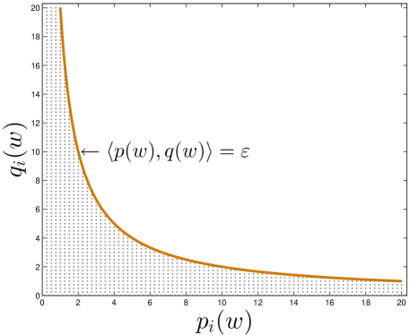
Figure 1: Effect of regularizing/smoothing the original optimization problem.

6 Experimental Validation

In this section, we demonstrate the effectiveness of our algorithms on five $\ell_{0}$ norm optimization tasks, namely feature selection, segmented regression, trend filtering, MRF optimization, and impulse noise removal. We compare our proposed MPEC-EPM (Algorithm 1) and MPEC-ADM (Algorithm 2) against the following methods.

• Greedy Hard Thresholding (GREEDY) (Beck and Eldar, 2013). It considers decreasing the objective function and identifying the active variables simultaneously using the following update: $\bm{\mathbf{x}}\Leftarrow\arg\min_{\|\bm{\mathbf{y}}\|_{0}\leq k}\|\bm{\mathbf{x}}-f^{\prime}(\bm{\mathbf{x}})/L_{f}-\bm{\mathbf{y}}\|_{2}^{2}$, where $L_{f}$ is the gradient Lipschitz continuity constant. Note that this method is not applicable when the objective is non-smooth.

• Gradient Support Pursuit (GSP). This is a state-of-the-art greedy algorithm that approximates sparse minima of cost functions which have stable restricted Hessian. We use the Matlab implementation provided by the author users.ece.gatech.edu/sbahmani7/GraSP.html.

• Convex $\ell_{1}$ minimization method (CVX). Since this approximate method can not control the sparsity of the solution, we solve a $\ell_{1}$ regularized problem where the regulation parameter is swept over $\{2^{-10},2^{-8},...,2^{10}\}$. Finally, the solution that leads to smallest objective value after a hard thresholding projection (which reduces to setting the smallest $n-k$ values of the solution in magnitude to 0) is selected.

• Quadratic Penalty Method (QPM) (Lu and Zhang, 2013). This is splitting method that introduces auxiliary variables to separate the calculation of the non-differentiable and differentiable term and then performs block coordinate descend on each subproblem. We use GREEDY to solve the subproblem with respect to $\bm{\mathbf{x}}$ with reasonable accuracy. We increase the penalty parameter by $\sqrt{10}$ in every $T=30$ iterations.

• Direct Alternating Direction Method (DI-ADM). This is an ADM directly applied to Eq (1). We use a similar experimental setting as QPM.

• Mean Doubly Alternating Direction Method (MD-ADM) (Dong and Zhang, 2013). This is an ADM that treats arithmetic means of the solution sequence as the actual output. We also use a similar parameter setting as QPM.

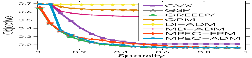
(a) ‘a6a’

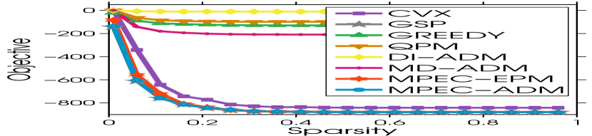
(b) ‘gisette’

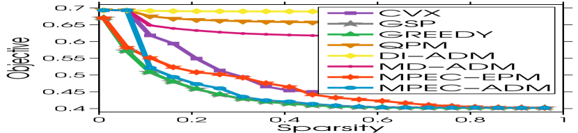
(c) ‘w2a’

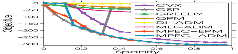
(d) ‘rcv1binary’

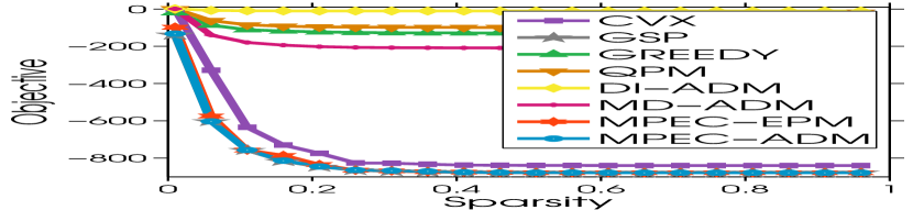
(e) ‘a5a’

(f) ‘realsim’

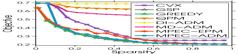
(g) ‘mushrooms’

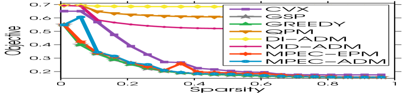
(h) ‘splice’

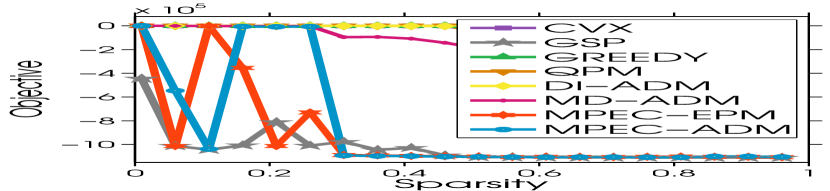
(i) ‘madelon’

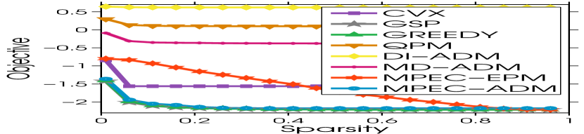
(j) ‘w1a’

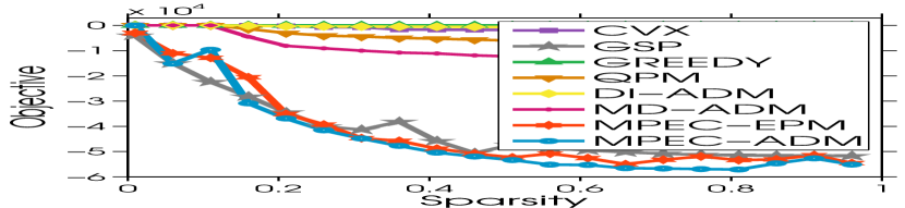
(k) ‘duke’

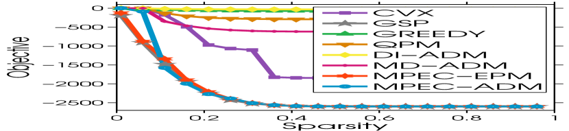
(l) ‘mnist’

Figure 2: Feature selection based on logistic loss minimization. We set $\lambda=0.01$.

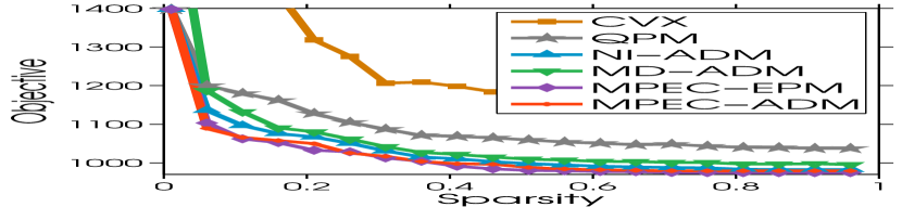
(a) ‘a6a’

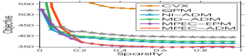
(b) ‘gisette’

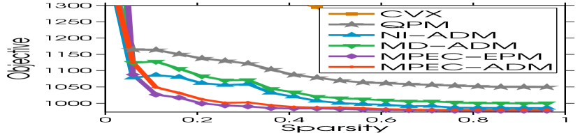
(c) ‘w2a’

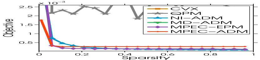
(d) ‘rcv1binary’

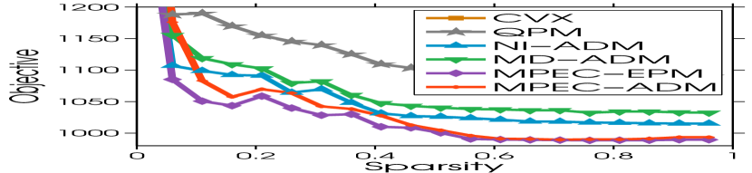
(e) ‘a5a’

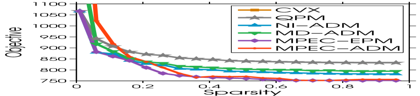
(f) ‘realsim’

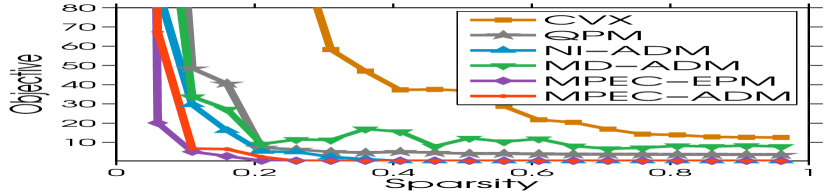
(g) ‘mushrooms’

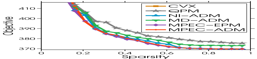
(h) ‘splice’

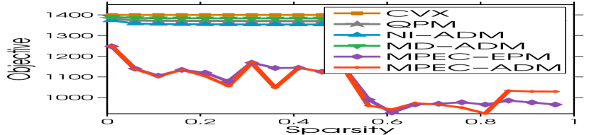
(i) ‘madelon’

(j) ‘w1a’

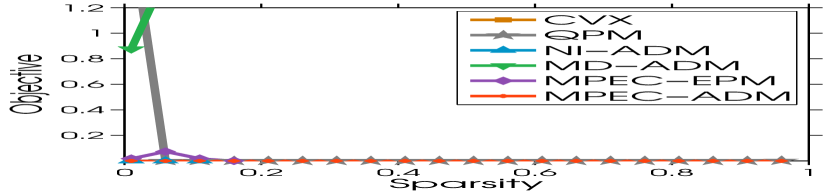
(k) ‘duke’

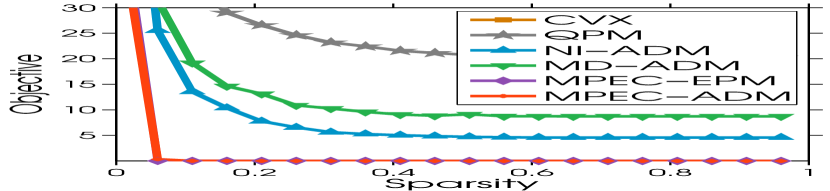
(l) ‘mnist’

Figure 3: Feature selection based on hinge loss minimization. We set $\lambda=0.01$.

We include the comparisons with GREEDY and GSP only on logistic loss feature selection, since these two methods are only applicable to smooth objectives. We vary the sparsity parameter $k=\{0.01,0.06,...,0.96\}\times n$ on different data sets and report the objective value of the optimization problem. All algorithms are implemented in Matlab on an Intel 2.6 GHz CPU with 128 GB RAM. We set $\rho^{0}=0.01$ for MPEC-EPM and $\alpha=\eta=0.01$ for MPEC-ADM. For the proximal parameter of both algorithms, we set $\mu=0.01$ .

6.1 Feature Selection

Given a set of labeled patterns $\{\bm{\mathbf{s}}_{i},\bm{\mathbf{y}}_{i}\}_{i=1}^{p}$, where $\bm{\mathbf{s}}_{i}$ is an instance with $n$ features and $\bm{\mathbf{y}}_{i}\in\{\pm 1\}$ is the label. Feature selection considers the following optimization problem:

$$\min_{\bm{\mathbf{x}}}~{}\textstyle\tfrac{\lambda}{2}\|\bm{\mathbf{x}}\|_{2}^{2}+\sum_{i}^{p}\ell\left(\langle\bm{\mathbf{s}}_{i},\bm{\mathbf{x}}\rangle,\bm{\mathbf{y}}_{i}\right),~{}s.t.~{}\|\bm{\mathbf{x}}\|_{0}\leq k$$ (45)

where the loss function $\ell(\cdot)$ is chosen to be the logistic loss: $\ell(r,t)=\log(1+\exp(r))-rt$ or the hinge loss: $\ell(r,t)=\max(0,1-rt)$.

In our experiments, we test on 12 well-known benchmark datasets which contain high dimensional ($n\geq 7000$) data vectors and thousands of data instances. Since we are solving an optimization problem, we only consider measuring the quality of the solutions by comparing the objective values.

Based on our experimental results in Figure 2, we make the following observations. (i) Convex methods generally gives good results in this task, but they fail on ‘duke’ and ‘madelon’ datasets. (ii) The quadratic penalization techniques (NI-ADM, MD-ADM and QPM) generally demonstrate bad performance in this task. (iii) GREEDY and GSP often achieve good performance, but they are not stable in some cases. (iv) Both our MPEC-EPM and MPEC-ADM often achieve better performance than existing solutions. For hinge loss feature selection, we demonstrate our experimental results in Figure 3. We make the following observations. (i) Convex methods generally fail in this situation, as they usually produce much larger objectives. (ii) NI-ADM and MD-ADM outperform QPM in all test cases. (iii) MPEC-EPM and MPEC-ADM generally achieve lower objective values.

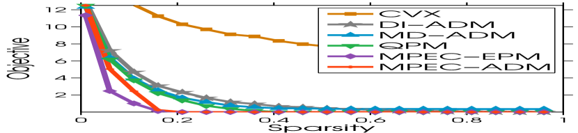
(a) $n=1024$, $\sigma=10$

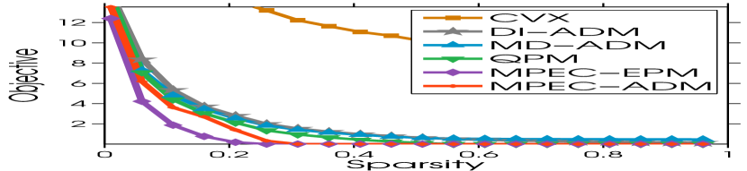
(b) $n=2048$, $\sigma=10$

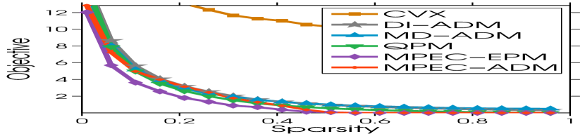
(c) $n=4096$, $\sigma=10$

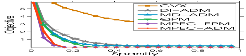
(d) $n=1024$, $\sigma=5$

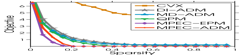
(e) $n=2048$, $\sigma=5$

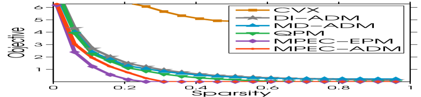
(f) $n=4096$, $\sigma=5$

Figure 4: Segmented regression. Results for unit-column-norm $\bm{\mathbf{A}}$ for different parameter settings.

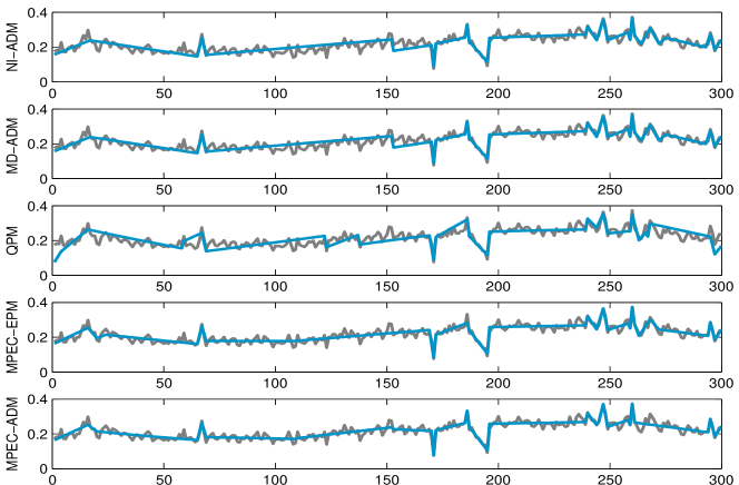
Figure 5: Trend filtering result on ‘snp500.dat’ data (Kim et al., 2009). The objective values achieved by the five methods are $0.38,0.38,0.53,0.32,0.33$, respectively.

6.2 Segmented Regression

Given a design matrix $\bm{\mathbf{A}}\in\mathbb{R}^{m\times n}$ and an observation vector $\bm{\mathbf{b}}\in\mathbb{R}^{m}$, segmented regression involves solving the following optimization problem:

$$\min_{\bm{\mathbf{x}}}~{}\textstyle\|\bm{\mathbf{A}}^{T}(\bm{\mathbf{A}}x-\bm{\mathbf{b}})\|_{\infty},~{}s.t.~{}\|\bm{\mathbf{x}}\|_{0}\leq k$$ (46)

This regression model is closely related to Dantzig selector (Candes and Tao, 2007) in the literature, where $\ell_{0}$ norm is replaced by $\ell_{1}$ norm in Eq (46). In our experiments, we consider design matrices with unit column norms. Similar to (Candes and Tao, 2007), we first generate an $\bm{\mathbf{A}}$ with independent Gaussian entries and then normalize each column to have norm 1. We then select a support set of size $0.5\times\min(m,n)$ uniformly at random. We finally set $\bm{\mathbf{b}}=\bm{\mathbf{Ax}}+\bm{\mathbf{\varepsilon}}$ with $\bm{\mathbf{\varepsilon}}\sim N(0,\sigma^{2}\bm{\mathbf{I}})$. We vary $n$ from $\{1024,2048,4096\}$ and set $m=n/8$. We demonstrate our experimental results in Figure 4. The proposed penalization techniques (MPEC-EPM and MPEC-ADM) outperform the quadratic penalization techniques (NI-ADM, MD-ADM and QPM) consistently.

6.3 Trend Filtering

Given a time series $\bm{\mathbf{y}}\in\mathbb{R}^{n}$, the goal of trend filtering is to find another nearest time series $\bm{\mathbf{x}}$ such that $\bm{\mathbf{x}}$ is sparse after a gradient mapping (Kim et al., 2009). Trend filtering involves solving the following optimization, where $\bm{\mathbf{D}}\in\mathbb{R}^{(n-2)\times n}$ is a $2^{\text{nd}}$ difference matrix.

$$\min_{\bm{\mathbf{x}}}~{}\textstyle\tfrac{1}{2}\|\bm{\mathbf{x}}-\bm{\mathbf{y}}\|_{2}^{2},~{}s.t.~{}\|\bm{\mathbf{Dx}}\|_{0}\leq k$$ (47)

In our experiments, we perform trend filtering on the ‘snp500.dat’ data set (Kim et al., 2009). For better visualization, we only use the first $300$ time instances of the signal $\bm{\mathbf{y}}$, i.e. $n=300$. The sparsity parameter $k$ is set to $30$. We stop all the algorithms when the same strict stopping criterion is met, in order to ensure that the hard constraint $\|\bm{\mathbf{Ax}}\|_{0}\leq k$ is fully satisfied. As shown in Figure 5, the proposed methods (MPEC-EPM and MPEC-ADM) achieve more natural trend filtering results (refer to position 120-170), since they achieve lower objective values (0.32 and 0.33).

(a) by Graph Cut
$f(\mathbf{x})=95741.1$

(b) by NI-ADM
$f(\mathbf{x})=95852.6$

(c) by MD-ADM
$f(\mathbf{x})=95825.2$

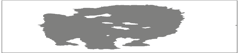
(d) by QPM
$f(\mathbf{x})=95827.3$

(e) by MPEC-EPM
$f(\mathbf{x})=95798.8$

(f) by MPEC-ADM
$f(\mathbf{x})=95748.0$

Figure 6: MRF optimization on ‘cat’ image. The objective value for the unary image $\bm{\mathbf{b}}$ is $f(\bm{\mathbf{b}})=96439.8$.

6.4 MRF Optimization

Markov Random Field (MRF) optimization involves solving the following problem (Kolmogorov and Zabih, 2004),

$$\min_{\bm{\mathbf{x}}}~{}\textstyle\frac{1}{2}\bm{\mathbf{x}}^{T}\bm{\mathbf{Lx}}+\bm{\mathbf{b}}^{T}\bm{\mathbf{x}},~{}s.t.~{}\bm{\mathbf{x}}\in\{0,1\}^{n}$$ (48)

where $\bm{\mathbf{b}}\in\mathbb{R}^{n}$ is determined by the unary term defined for the graph and $\bm{\mathbf{L}}\in\mathbb{R}^{n\times n}$ is the Laplacian matrix, which is based on the binary term relating pairs of graph nodes together. The quadratic term is usually considered a smoothness prior on the node labels. The MRF formulation is widely used in many labeling applications, including image segmentation.

In our experiments, we include the comparison with the graph cut method (Kolmogorov and Zabih, 2004), which is known to achieve the global optimal solution for this specific class of binary problem. Figure 6 demonstrates a qualitative result for image segmentation. MPEC-ADM produces a solution that is very close to the globally optimal one. Moreover, both our methods achieve lower objectives than the other compared methods.

Table 2: Random-value impulse noise removal problems. The results separated by ‘/’ are $SNR_{0}$, $SNR_{1}$ and $SNR_{2}$, respectively.

	CVX (i.e. $\ell_{1}TV$)	DI-ADM	MD-ADM	QPM	MPEC-EPM	MPEC-ADM
mandrill+10%	0.83/3.06/5.00	0.78/3.68/7.06	0.84/3.71/7.10	0.85/3.76/7.16	0.85/3.71/6.90	0.86/3.87/7.64
mandrill+30%	0.69/2.38/4.42	0.67/2.96/5.13	0.74/2.91/4.96	0.75/2.94/5.02	0.75/2.89/4.87	0.76/3.02/5.13
mandrill+50%	0.55/1.80/3.33	0.58/2.32/3.86	0.65/2.23/3.64	0.66/2.30/3.79	0.66/2.22/3.58	0.67/2.39/3.88
mandrill+70%	0.41/0.91/1.64	0.47/1.49/2.42	0.52/1.39/2.17	0.52/1.40/2.22	0.53/1.39/2.12	0.55/1.56/2.43
mandrill+90%	0.31/0.02/0.09	0.33/0.14/0.13	0.35/0.04/-0.08	0.35/0.04/-0.03	0.36/0.07/-0.14	0.37/0.19/0.05
lenna+10%	0.97/8.08/13.48	0.97/8.05/13.51	0.97/8.13/13.59	0.97/8.12/13.87	0.97/8.10/13.72	0.98/8.31/14.55
lenna+30%	0.92/7.40/13.60	0.92/6.71/10.53	0.91/6.62/10.07	0.94/7.38/12.27	0.93/7.19/11.86	0.96/7.90/13.68
lenna+50%	0.84/5.50/9.46	0.84/5.32/8.13	0.83/5.18/7.53	0.88/6.28/10.10	0.86/5.75/8.69	0.91/6.65/10.89
lenna+70%	0.57/2.48/4.17	0.67/3.34/5.11	0.66/3.17/4.40	0.71/3.66/5.34	0.69/3.34/4.53	0.75/4.09/5.81
lenna+90%	0.35/0.53/0.89	0.41/0.76/0.91	0.40/0.54/0.48	0.41/0.66/0.80	0.43/0.54/0.38	0.48/0.89/0.80
lake+10%	0.94/8.03/14.66	0.95/8.21/13.64	0.96/8.31/13.81	0.96/8.40/14.52	0.96/8.33/14.14	0.96/8.45/14.72
lake+30%	0.88/7.29/12.83	0.86/6.86/10.87	0.87/6.81/10.02	0.91/7.57/12.45	0.89/7.26/11.33	0.92/7.87/13.34
lake+50%	0.61/4.89/8.31	0.76/5.69/8.52	0.77/5.65/8.02	0.83/6.57/10.36	0.80/5.98/8.78	0.85/6.75/10.56
lake+70%	0.40/2.07/3.61	0.51/3.68/5.49	0.56/3.72/5.14	0.60/4.01/5.60	0.61/3.94/5.28	0.62/4.08/5.61
lake+90%	0.27/0.54/0.87	0.25/0.94/1.06	0.27/0.87/0.65	0.26/0.75/0.65	0.29/0.81/0.44	0.28/0.90/0.71
jetplane+10%	0.42/3.33/7.98	0.37/3.16/7.10	0.39/3.16/7.15	0.39/3.20/7.43	0.39/3.16/7.28	0.39/3.22/7.52
jetplane+30%	0.36/2.94/7.00	0.35/2.70/5.69	0.38/2.68/5.60	0.39/2.98/6.68	0.39/2.87/6.24	0.40/3.14/7.23
jetplane+50%	0.26/1.75/4.24	0.31/2.02/4.21	0.37/2.08/4.00	0.38/2.56/5.45	0.37/2.26/4.48	0.40/2.72/5.75
jetplane+70%	0.24/-0.55/-0.17	0.24/0.62/1.46	0.31/0.83/1.49	0.30/0.81/1.44	0.34/0.98/1.55	0.33/0.92/1.38
jetplane+90%	0.19/-1.81/-3.38	0.17/-1.98/-3.23	0.18/-1.96/-3.47	0.18/-2.18/-3.90	0.20/-1.66/-2.13	0.19/-2.05/-3.80
blonde+10%	0.26/0.92/2.83	0.25/0.87/2.69	0.25/0.86/2.68	0.22/0.90/2.80	0.27/0.88/2.72	0.25/0.92/2.87
blonde+30%	0.25/0.82/2.57	0.26/0.76/2.21	0.26/0.70/2.14	0.25/0.80/2.47	0.27/0.76/2.35	0.27/0.85/2.59
blonde+50%	0.25/0.60/1.89	0.25/0.61/1.80	0.24/0.58/1.77	0.25/0.67/2.13	0.25/0.64/1.96	0.26/0.75/2.26
blonde+70%	0.24/0.02/0.22	0.22/0.35/1.02	0.21/0.35/1.05	0.22/0.33/1.11	0.20/0.38/1.19	0.26/0.49/1.47
blonde+90%	0.20/-0.81/-1.39	0.21/-0.62/-1.15	0.20/-0.65/-1.26	0.18/-0.75/-1.39	0.20/-0.52/-1.03	0.19/-0.45/-0.88

6.5 Impulse Noise Removal

Given a noisy image $\bm{\mathbf{b}}$ which was contaminated by random value impulsive noise, we consider a denoised image of $\bm{\mathbf{x}}$ as a minimizer of the following constrained $\ell_{0}TV$ model (Yuan and Ghanem, 2015):

$$\min_{\bm{\mathbf{x}}}~{}TV(\bm{\mathbf{x}}),~{}s.t.~{}\|\bm{\mathbf{x}}-\bm{\mathbf{b}}\|_{0}\leq k$$ (49)

where $TV(\bm{\mathbf{x}})\triangleq\|\bm{\mathbf{\nabla}}\bm{\mathbf{x}}\|_{p,1}$ denotes the total variation norm function, $\|\bm{\mathbf{x}}\|_{p,1}\triangleq\sum_{i=1}^{n}(|\bm{\mathbf{x}}_{i}|^{p}+|\bm{\mathbf{x}}_{n+i}|^{p})^{\frac{1}{p}};~{}\bm{\mathbf{\nabla}}\triangleq\left[\bm{\mathbf{\nabla}}_{x}|\bm{\mathbf{\nabla}}_{y}\right]^{T}\in\mathbb{R}^{2n\times n}$, and $k$ specifies the noise level. Furthermore, $\bm{\mathbf{\nabla}}_{x}\in\mathbb{R}^{n\times n}$ and $\bm{\mathbf{\nabla}}_{y}\in\mathbb{R}^{n\times n}$ are two suitable linear transformation matrices that computes their discrete gradients. Following the experimental settings in (Yuan and Ghanem, 2015), we use three ways to measure SNR, i.e. $SNR_{0},SNR_{1},SNR_{2}$. We show image recovery results in Table 2 when random-value impulse noise is added to the clean images {‘mandrill’, ‘lenna’, ‘lake’, ‘jetplane’, ‘blonde’}. We also demonstrate a visualized example of random value impulse noise removal on ‘lenna’ image in Figure 7. A conclusion can be drawn that both MPEC-EPM and MPEC-ADM achieve state-of-the-art performance while MPEC-ADM is generally better than MPEC-EPM in this impulse noise removal problem.

(a) by CVX
   $SNR_{0}=0.92$

(b) by NI-ADM
   $SNR_{0}=0.92$

(c) by MD-ADM
   $SNR_{0}=0.91$

(d) by QPM
   $SNR_{0}=0.94$

(e) by MPEC-EPM
   $SNR_{0}=0.93$

(f) by MPEC-ADM
   $SNR_{0}=0.96$

Figure 7: Random value impulse noise removal on ‘lenna’ image.

7 Conclusions

This paper presents two methods (exact penalty and alternating direction) to solve the general sparsity constrained minimization problem. Although it is non-convex, we design effective penalization/regularization schemes to solve its equivalent MPEC. We also prove that both of our methods are convergent to first-order KKT points. Experimental results on a variety of sparse optimization applications demonstrate that our methods achieve state-of-the-art performance.

Appendix

A Matlab Code of Breakpoint Search Algorithm

In this section, we include a Matlab implementation of the breakpoint search algorithm (Helgason et al., 1980) which solves the optimization problem in Eq (50) exactly in $n\log(n)$ time.

$$\min_{\bm{\mathbf{x}}}~{}\frac{1}{2}\bm{\mathbf{x}}^{T}diag(d)\bm{\mathbf{x}}+\bm{\mathbf{x}}^{T}\bm{\mathbf{a}},~{}s.t.~{}\bm{\mathbf{0}}\leq\bm{\mathbf{x}}\leq\bm{\mathbf{1}},~{}\bm{\mathbf{x}}^{T}\bm{\mathbf{1}}~{}\lesseqqgtr~{}s$$ (50)

where $\bm{\mathbf{x}},\bm{\mathbf{d}},\bm{\mathbf{a}}\in\mathbb{R}^{n}$, $\bm{\mathbf{d}}>0$, and $0\leq s\leq n$. In addition, $\lesseqqgtr$ is a comparison operator, and it can be strict equal operator (=), greater than or equal operator ($\geq$), or less than or equal operator ($\leq$). We list our code as follows.

⬇

function [x] = BreakPointSearch(d,a,s,oper)

% This program solves the following QP:

% min_x 0.5*x’*diag(d)*x + a’*x

% s.t. sum(x) oper s, 0 <= x <= 1

% oper can be ’==’, ’>=’, or ’<=’

% We assume d > 0.

n = length(d);assert( s>=0 && s<=n );

y = sort([-a-d;-a],’ascend’);

l = 1; r = 2*n; L = n; R = 0;

while 1

if(r-l==1)

S = (s-L)/(R-L);

rho = y(l)+(y(r) - y(l))*S;

break;

else

m = floor(0.5*(l+r));

t = (-a-y(m))./d;

C = sum(max(0,min(t,1)));

if(C==s),

rho = y(m);break;

elseif(C>s)

l = m;L=C;

elseif(C<s)

r = m;R=C;

end

end

end

if (oper(1)==’>’)

rho = min(rho,0);

elseif(oper(1)==’<’)

rho = max(rho,0);

end

t = (-a-rho)./d;

x = max(0,min(t,1));

References

- Argyriou et al. (2012) Andreas Argyriou, Rina Foygel, and Nathan Srebro. Sparse prediction with the -support norm. In Neural Information Processing Systems (NIPS), pages 1466–1474, 2012.
- Attouch et al. (2010) Hedy Attouch, Jérôme Bolte, Patrick Redont, and Antoine Soubeyran. Proximal alternating minimization and projection methods for nonconvex problems: An approach based on the kurdyka-lojasiewicz inequality. Mathematics of Operations Research (MOR), 35(2):438–457, 2010.
- Bahmani et al. (2013) Sohail Bahmani, Bhiksha Raj, and Petros T. Boufounos. Greedy sparsity-constrained optimization. Journal of Machine Learning Research (JMLR), 14(1):807–841, 2013.
- Bao et al. (2016) Chenglong Bao, Hui Ji, Yuhui Quan, and Zuowei Shen. Dictionary learning for sparse coding: Algorithms and convergence analysis. IEEE Transactions on Pattern Analysis and Machine Intelligence (TPAMI), 38(7):1356–1369, 2016.
- Beck and Eldar (2013) Amir Beck and Yonina C Eldar. Sparsity constrained nonlinear optimization: Optimality conditions and algorithms. SIAM Journal on Optimization (SIOPT), 23(3):1480–1509, 2013.
- Bertsimas et al. (2015) Dimitris Bertsimas, Angela King, and Rahul Mazumder. Best subset selection via a modern optimization lens. arXiv preprint:1507.03133, 2015.
- Bi (2014) Shujun Bi. Study for multi-stage convex relaxation approach to low-rank optimization problems, phd thesis, south china university of technology. 2014.
- Bi and Pan (2017) Shujun Bi and Shaohua Pan. Multistage convex relaxation approach to rank regularized minimization problems based on equivalent mathematical program with a generalized complementarity constraint. SIAM Journal on Control and Optimization (SICON), 55(4):2493–2518, 2017.
- Bi et al. (2014) Shujun Bi, Xiaolan Liu, and Shaohua Pan. Exact penalty decomposition method for zero-norm minimization based on MPEC formulation. SIAM Journal on Scientific Computing (SISC), 36(4), 2014.
- Bienstock (1996) Daniel Bienstock. Computational study of a family of mixed-integer quadratic programming problems. Mathematical programming, 74(2):121–140, 1996.
- Blumensath and Davies (2008) Thomas Blumensath and Mike E Davies. Gradient pursuits. IEEE Transactions on Signal Processing, 56(6):2370–2382, 2008.
- Bolte et al. (2014) Jérôme Bolte, Shoham Sabach, and Marc Teboulle. Proximal alternating linearized minimization for nonconvex and nonsmooth problems. Mathematical Programming, 146(1-2):459–494, 2014.
- Candes and Tao (2007) Emmanuel Candes and Terence Tao. The dantzig selector: statistical estimation when p is much larger than n. The Annals of Statistics, pages 2313–2351, 2007.
- Candès and Tao (2005) Emmanuel J. Candès and Terence Tao. Decoding by linear programming. IEEE Transactions on Information Theory, 51(12):4203–4215, 2005.
- Candes et al. (2008) Emmanuel J Candes, Michael B Wakin, and Stephen P Boyd. Enhancing sparsity by reweighted minimization. Journal of Fourier Analysis and Applications, 14(5-6):877–905, 2008.
- Chan et al. (2007) Antoni B. Chan, Nuno Vasconcelos, and Gert R. G. Lanckriet. Direct convex relaxations of sparse svm. In International Conference on Machine Learning (ICML), pages 145–153, 2007.
- Chen et al. (1998) Scott Shaobing Chen, David L Donoho, and Michael A Saunders. Atomic decomposition by basis pursuit. SIAM journal on Scientific Computing (SISC), 20(1):33–61, 1998.
- Dattorro (2011) Jon Dattorro. Convex Optimization & Euclidean Distance Geometry. Meboo Publishing USA, 2011.
- DeMiguel et al. (2005) Victor DeMiguel, Michael P Friedlander, Francisco J Nogales, and Stefan Scholtes. A two-sided relaxation scheme for mathematical programs with equilibrium constraints. SIAM Journal on Optimization (SIOPT), 16(2):587–609, 2005.
- Dong and Zhang (2013) Bin Dong and Yong Zhang. An efficient algorithm for l0 minimization in wavelet frame based image restoration. Journal of Scientific Computing, 54(2-3):350–368, 2013.
- Donoho (2006) David L Donoho. Compressed sensing. IEEE Transactions on Information Theory, 52(4):1289–1306, 2006.
- Duchi et al. (2008) John C. Duchi, Shai Shalev-Shwartz, Yoram Singer, and Tushar Chandra. Efficient projections onto the ball for learning in high dimensions. In International Conference on Machine Learning (ICML), pages 272–279, 2008.
- Elhamifar and Vidal (2009) Ehsan Elhamifar and René Vidal. Sparse subspace clustering. In Computer Vision and Pattern Recognition (CVPR), pages 2790–2797, 2009.
- Facchinei et al. (1999) Francisco Facchinei, Houyuan Jiang, and Liqun Qi. A smoothing method for mathematical programs with equilibrium constraints. Mathematical programming, 85(1):107–134, 1999.
- Fan and Li (2001) Jianqing Fan and Runze Li. Variable selection via nonconcave penalized likelihood and its oracle properties. Journal of the American Statistical Association (JASA), 96(456):1348–1360, 2001.
- Feng et al. (2013) Mingbin Feng, John E Mitchell, Jong-Shi Pang, Xin Shen, and Andreas Wachter. Complementarity formulations of -norm optimization problems. 2013.
- Fogel et al. (2015) Fajwel Fogel, Rodolphe Jenatton, Francis R. Bach, and Alexandre d’Aspremont. Convex relaxations for permutation problems. SIAM Journal on Matrix Analysis and Applications (SIMAX), 36(4):1465–1488, 2015.
- Friedman et al. (2008) Jerome Friedman, Trevor Hastie, and Robert Tibshirani. Sparse inverse covariance estimation with the graphical lasso. Biostatistics, 9(3):432–441, 2008.
- Friedman (2012) Jerome H Friedman. Fast sparse regression and classification. International Journal of Forecasting, 28(3):722–738, 2012.
- Gao et al. (2011) Cuixia Gao, Naiyan Wang, Qi Yu, and Zhihua Zhang. A feasible nonconvex relaxation approach to feature selection. In AAAI Conference on Artificial Intelligence (AAAI), pages 356–361, 2011.
- Ge et al. (2011) Dongdong Ge, Xiaoye Jiang, and Yinyu Ye. A note on the complexity of minimization. Mathematical Programming, 129(2):285–299, 2011.
- Geman and Yang (1995) Donald Geman and Chengda Yang. Nonlinear image recovery with half-quadratic regularization. IEEE Transactions on Image Processing (TIP), 4(7):932–946, 1995.
- Gong et al. (2013) Pinghua Gong, Changshui Zhang, Zhaosong Lu, Jianhua Huang, and Jieping Ye. A general iterative shrinkage and thresholding algorithm for non-convex regularized optimization problems. In International Conference on Machine Learning (ICML), pages 37–45, 2013.
- He and Yuan (2012) Bingsheng He and Xiaoming Yuan. On the convergence rate of the douglas-rachford alternating direction method. SIAM Journal on Numerical Analysis (SINUM), 50(2):700–709, 2012.
- Helgason et al. (1980) Richard V. Helgason, Jeffery L. Kennington, and H. S. Lall. A polynomially bounded algorithm for a singly constrained quadratic program. Mathematical Programming, 18(1):338–343, 1980.
- Hu and Ralph (2004) XM Hu and Daniel Ralph. Convergence of a penalty method for mathematical programming with complementarity constraints. Journal of Optimization Theory and Applications, 123(2):365–390, 2004.
- Jain et al. (2014) Prateek Jain, Ambuj Tewari, and Purushottam Kar. On iterative hard thresholding methods for high-dimensional m-estimation. In Neural Information Processing Systems (NIPS), pages 685–693, 2014.
- Jiang et al. (2015) Bo Jiang, Ya-Feng Liu, and Zaiwen Wen. -norm regularization algorithms for optimization over permutation matrices. Technical report, Optimization online, November 2015.
- Kadrani et al. (2009) Abdeslam Kadrani, Jean-Pierre Dussault, and Abdelhamid Benchakroun. A new regularization scheme for mathematical programs with complementarity constraints. SIAM Journal on Optimization (SIOPT), 20(1):78–103, 2009.
- Kim et al. (2009) Seung-Jean Kim, Kwangmoo Koh, Stephen P. Boyd, and Dimitry M. Gorinevsky. trend filtering. SIAM Review, 51(2):339–360, 2009.
- Kolmogorov and Zabih (2004) Vladimir Kolmogorov and Ramin Zabih. What energy functions can be minimized via graph cuts? IEEE Transactions on Pattern Analysis and Machine Intelligence (TPAMI), 26(2):147–159, 2004.
- Lee et al. (2006) Honglak Lee, Alexis Battle, Rajat Raina, and Andrew Y. Ng. Efficient sparse coding algorithms. In Neural Information Processing Systems (NIPS), pages 801–808, 2006.
- Li et al. (2004) Yuanqing Li, Andrzej Cichocki, and Shun-ichi Amari. Analysis of sparse representation and blind source separation. Neural computation, 16(6):1193–1234, 2004.
- Liu et al. (2015) Ya-Feng Liu, Yu-Hong Dai, and Shiqian Ma. Joint power and admission control: Non-convex l approximation and an effective polynomial time deflation approach. IEEE Transactions on Signal Processing, 63(14):3641–3656, 2015.
- Lu et al. (2014) Canyi Lu, Jinhui Tang, Shuicheng Yan, and Zhouchen Lin. Generalized nonconvex nonsmooth low-rank minimization. In Conference on Computer Vision and Pattern Recognition (CVPR), pages 4130–4137, 2014.
- Lu and Zhang (2013) Zhaosong Lu and Yong Zhang. Sparse approximation via penalty decomposition methods. SIAM Journal on Optimization (SIOPT), 23(4):2448–2478, 2013.
- Luo et al. (1996) Zhi-Quan Luo, Jong-Shi Pang, and Daniel Ralph. Mathematical programs with equilibrium constraints. Cambridge University Press, 1996.
- Mairal et al. (2010) Julien Mairal, Francis Bach, Jean Ponce, and Guillermo Sapiro. Online learning for matrix factorization and sparse coding. Journal of Machine Learning Research (JMLR), 11(Jan):19–60, 2010.
- Mallat and Zhang (1993) Stéphane G Mallat and Zhifeng Zhang. Matching pursuits with time-frequency dictionaries. IEEE Transactions on Signal Processing, 41(12):3397–3415, 1993.
- Mazumder et al. (2012) Rahul Mazumder, Jerome H Friedman, and Trevor Hastie. Sparsenet: Coordinate descent with nonconvex penalties. Journal of the American Statistical Association (JASA), 2012.
- McDonald et al. (2014) Andrew M McDonald, Massimiliano Pontil, and Dimitris Stamos. Spectral -support norm regularization. In Neural Information Processing Systems (NIPS), pages 3644–3652, 2014.
- Needell and Tropp (2009) Deanna Needell and Joel A Tropp. Cosamp: Iterative signal recovery from incomplete and inaccurate samples. Applied and Computational Harmonic Analysis, 26(3):301–321, 2009.
- Needell and Vershynin (2009) Deanna Needell and Roman Vershynin. Uniform uncertainty principle and signal recovery via regularized orthogonal matching pursuit. Foundations of computational mathematics, 9(3):317–334, 2009.
- Ng (2004) Andrew Y Ng. Feature selection, vs. regularization, and rotational invariance. In International Conference on Machine Learning (ICML), page 78, 2004.
- Pilanci et al. (2015) Mert Pilanci, Martin J. Wainwright, and Laurent El Ghaoui. Sparse learning via boolean relaxations. Mathematical Programming, 151(1):63–87, 2015.
- Rao et al. (2015) Nikhil S. Rao, Parikshit Shah, and Stephen J. Wright. Forward-backward greedy algorithms for atomic norm regularization. IEEE Transactions on Signal Processing, 63(21):5798–5811, 2015.
- Tropp et al. (2007) Joel Tropp, Anna C Gilbert, et al. Signal recovery from random measurements via orthogonal matching pursuit. IEEE Transactions on Information Theory, 53(12):4655–4666, 2007.
- Tropp (2004) Joel A. Tropp. Greed is good: algorithmic results for sparse approximation. IEEE Transactions on Information Theory, 50(10):2231–2242, 2004.
- Trzasko and Manduca (2009) Joshua Trzasko and Armando Manduca. Highly undersampled magnetic resonance image reconstruction via homotopic-minimization. IEEE Transactions on Medical Imaging, 28(1):106–121, 2009.
- Wang et al. (2013) Peng Wang, Chunhua Shen, and Anton van den Hengel. A fast semidefinite approach to solving binary quadratic problems. In Computer Vision and Pattern Recognition (CVPR), pages 1312–1319, 2013.
- Weinmann et al. (2015) Andreas Weinmann, Martin Storath, and Laurent Demaret. The -potts functional for robust jump-sparse reconstruction. SIAM Journal on Numerical Analysis (SINUM), 53(1):644–673, 2015.
- Weston et al. (2003) Jason Weston, André Elisseeff, Bernhard Schölkopf, and Michael E. Tipping. Use of the zero-norm with linear models and kernel methods. Journal of Machine Learning Research (JMLR), 3:1439–1461, 2003.
- Wu et al. (2014) Bin Wu, Chao Ding, Defeng Sun, and Kim-Chuan Toh. On the moreau-yosida regularization of the vector k-norm related functions. SIAM Journal on Optimization (SIOPT), 24(2):766–794, 2014.
- Xiang et al. (2009) Zhen James Xiang, Yongxin Taylor Xi, Uri Hasson, and Peter J. Ramadge. Boosting with spatial regularization. In Neural Information Processing Systems (NIPS), pages 2107–2115, 2009.
- Xu et al. (2011) Li Xu, Cewu Lu, Yi Xu, and Jiaya Jia. Image smoothing via gradient minimization. ACM Transactions on Graphics (TOG), 30(6):174, 2011.
- Yin et al. (2015) Penghang Yin, Yifei Lou, Qi He, and Jack Xin. Minimization of for compressed sensing. SIAM Journal on Scientific Computing (SISC), 37(1), 2015.
- Yu et al. (2011) Jin Yu, Anders Eriksson, Tat-Jun Chin, and David Suter. An adversarial optimization approach to efficient outlier removal. In International Conference on Computer Vision (ICCV), pages 399–406, 2011.
- Yuan and Ghanem (2015) Ganzhao Yuan and Bernard Ghanem. : A new method for image restoration in the presence of impulse noise. In Computer Vision and Pattern Recognition (CVPR), pages 5369–5377, 2015.
- Yuan and Ghanem (2016a) Ganzhao Yuan and Bernard Ghanem. Binary optimization via mathematical programming with equilibrium constraints. arXiv preprint arXiv:1608.04425, 2016a.
- Yuan and Ghanem (2016b) Ganzhao Yuan and Bernard Ghanem. A proximal alternating direction method for semi-definite rank minimization. In AAAI Conference on Artificial Intelligence (AAAI), 2016b.
- Yuan (2010) Ming Yuan. High dimensional inverse covariance matrix estimation via linear programming. The Journal of Machine Learning Research (JMLR), 11:2261–2286, 2010.
- Yuan et al. (2014) Xiaotong Yuan, Ping Li, and Tong Zhang. Gradient hard thresholding pursuit for sparsity-constrained optimization. In International Conference on Machine Learning (ICML), pages 127–135, 2014.
- Zhang (2010a) Cun-Hui Zhang. Nearly unbiased variable selection under minimax concave penalty. The Annals of statistics, pages 894–942, 2010a.
- Zhang (2010b) Tong Zhang. Analysis of multi-stage convex relaxation for sparse regularization. The Journal of Machine Learning Research (JMLR), 11:1081–1107, 2010b.
- Zhang (2011) Tong Zhang. Adaptive forward-backward greedy algorithm for learning sparse representations. IEEE Transactions on Information Theory, 57(7):4689–4708, 2011.
- Zou (2006) Hui Zou. The adaptive lasso and its oracle properties. Journal of the American statistical association, 101(476):1418–1429, 2006.
- Zou and Hastie (2005) Hui Zou and Trevor Hastie. Regularization and variable selection via the elastic net. Journal of the Royal Statistical Society: Series B (Statistical Methodology), 67(2):301–320, 2005.