Attribute Extraction from Product Titles in eCommerce

Abstract

This paper presents a named entity extraction system for detecting attributes in product titles of eCommerce retailers like Walmart. The absence of syntactic structure in such short pieces of text makes extracting attribute values a challenging problem. We find that combining sequence labeling algorithms such as Conditional Random Fields and Structured Perceptron with a curated normalization scheme produces an effective system for the task of extracting product attribute values from titles. To keep the discussion concrete, we will illustrate the mechanics of the system from the point of view of a particular attribute - brand. We also discuss the importance of an attribute extraction system in the context of retail websites with large product catalogs, compare our approach to other potential approaches to this problem and end the paper with a discussion of the performance of our system for extracting attributes.

1 Introduction

1.1 Vocabulary

Before beginning the discussion of the problem we will first define some terms that will be used in the remainder of the paper. A product is any commodity which may be sold by a retailer. An attribute is a feature that describes a specific property of a product or a product listing. Some examples of attributes include brand, color, gender, material, title, description, etc. An attribute value is a particular value assumed by the attribute. For example, for the product title

Apple iPad Mini 3 16GB Wi-Fi Refurbished, Gold

the brand attribute value is ‘Apple’ and the color attribute value is ‘Gold’. A product may alternatively be defined as a collection of such attribute-value pairs, where a value can potentially be empty. Formally, let $\mathfrak{p}$ be a product with attributes $\alpha_{1},\alpha_{2},...,\alpha_{m}$ and values $v_{1},v_{2},...,v_{m}$ respectively. Then, we represent $\mathfrak{p}=\{\alpha_{1}:v_{1},\alpha_{2}:v_{2},...,\alpha_{m}:v_{m}\}$ and write $\mathfrak{p}(\alpha_{i})=v_{i}$ for $1\leq i\leq m$ to indicate an attribute-value relationship for $\mathfrak{p}$.

In the context of an eCommerce website, the attribute values may be used to filter search results based on the items with a matching attribute value. As is done on Walmart.com and several other retail websites, this may be accomplished by populating relevant attribute values in the left hand navigation pane. For any given search or browse session, the attributes that are displayed for further filtering in the left hand navigation as described above will be called facets.

For the sake of brevity, we use the terms ‘attribute value extraction’ and ‘attribute extraction’ synonymously.

1.2 Problem set up

We formalize attribute extraction as per the following definition.

Definition 1.

Let $x$ be a product title and let $(x_{1},x_{2},..,x_{n})$ be a particular tokenization $\mathbf{x}_{\mathbf{t}}$ of $x$. Given an attribute $\alpha$, attribute extraction is the process of discovering two functions $E$ (raw extraction) and $N$ (normalization) such that

• $E(\mathbf{x_{t}})=E((x_{1},x_{2},...,x_{n}))=(x_{i},x_{i+1},...,x_{k})$ for $1\leq i\leq k\leq n$ where $\mathbf{a}_{\mathbf{v}}=(x_{i},x_{i+1},...,x_{k})$ is a tokenization of a particular value of $\alpha$,

• $N((x_{i},x_{i+1},...,x_{k}))=a_{s}$ where $a_{s}$ is the standardized representation of $\mathbf{a_{v}}$.

Example 1.

Consider the product title

$x=$ Hewlett Packard B4L03A#B1H Officejet Pro Eaio

so that whitespace tokenization yields

$$\mathbf{x_{t}}=(x_{1},x_{2},...,x_{6})=(\text{Hewlett, Packard, ..., Eaio}).$$

Let $\alpha$ be the attribute ‘brand’. Then we seek to find two functions $E$ and $N$ such that

$$E((x_{1},x_{2},...,x_{6}))=(x_{1},x_{2})=(\text{Hewlett, Packard})$$

and

$$N((\text{Hewlett, Packard}))=HP.$$

The goal of the attribute extraction system is to minimize the loss function $1-F_{1}$ where the $F_{1}$ measure is as defined in section 9.1.

Attribute value extraction is a particular instance of a named entity recognition problem. This paper explores the use of machine learning techniques, in particular, sequence labeling algorithms for the purposes of extracting attribute values from product titles. We will also illustrate a normalization scheme which provides the dual benefits of standardizing variations in the same attribute value and boosting precision.

In section 3, we outline some of the challenges associated with attribute extraction in general. We reference some of the previous work on the problem of entity extraction in section 4. Section 5 describes the sequence labeling algorithms used to build an attribute extraction system that works well with eCommerce data. This system is described in detail in sections 6 - 9 with respect to a particular attribute - ‘brand’. We finish the paper by describing how similar approaches have been successful in extracting other attributes such as ’character’, ‘manufacturer part number’, ‘package quantity’, etc and discussing the importance of attribute extraction in eCommerce.

2 Use Cases

In this section, we elaborate on the importance of attribute extraction for retail websites.

2.1 Discoverability

Using facets to filter search or browse results is a common way for consumers of eCommerce websites to navigate the site and search through the product space. In order to ensure a good faceted navigation experience, it is critical to associate attribute value metadata to products for the attributes that appear in the facets.

For example, let $S$ be a search query entered by a user and $\mathcal{R}$ be the set of products returned as a result. Suppose product $\mathfrak{p}\in\mathcal{R}$ and $\mathfrak{p}$ has an attribute $\alpha$ which also happens to be a facet. Suppose further that the value of $\alpha$ applicable to $\mathfrak{p}$ is $v$. When the user clicks on facet value $v$, the filtered result set is $\mathcal{R}^{{}^{\prime}}\subseteq\mathcal{R}$. Then $\mathfrak{p}\in\mathcal{R}^{{}^{\prime}}$ if and only if $\mathfrak{p}(\alpha)=v$. More concretely, suppose a user enters the search query ‘Tee shirt’ and the result set contains the product titled

Hanes Mens NANO-T Dri T-Shirt S Deep Red

However, if the attribute ‘color’ for the product is missing the value ‘Red’, then if the user clicks on the value ‘Red’ under facet ‘color’, this product will no longer show in the result set even though it has the attribute value of interest to the user.

Thus, absence of relevant attribute values in product metadata has a direct bearing on the discoverability of the product and ultimately funnels down to affect the sale of such products.

It is crucial for modern eCommerce sites to be able to add products to its catalog as quickly as possible. As such, in order to ensure that the item set up process has minimal requirements, providing attribute values may not be enforced for all attributes. Consequently, a large fraction of incoming product data may not have attribute values supplied. In the absence of a system to tag missing attribute values, the discoverability of such products will be diminished.

2.2 Ad campaigns

Certain attribute values are also are required by ad publishers such as Google and Bing in order to launch ad campaigns for products. In the absence of the required attributes, the ad campaigns are rejected.

2.3 Compliance

Some attribute values are necessary to satisfy government compliance requirements, e.g. unit price for food items or items sold in bulk.

2.4 Knowledge discovery

The list of valid values for a particular attribute may not be fixed. This is true, for instance, with attributes like ‘brand’, ‘character’, ‘model number’, etc. It is desirable to build a solution that can discover attribute values not currently part of the knowledge base.

3 Challenges

3.1 Extracting attributes from product titles

We will describe a sequence labeling based machine learning system for extracting values of certain product attributes from product titles. We will discuss the challenges associated with this task and how they were handled in the current solution. In the next few sections we will describe the attribute extraction system using the specific example of brand extraction.

In certain product categories, brand is an important attribute. Extracting brands from product titles presents several interesting challenges, some of which are outlined below. Whenever possible, we include examples of actual titles of products sold on Walmart.com. In later sections we discuss how our solution mitigates these issues.

• Unlike English prose, product titles do not adhere to a syntactic structure. They may be a concatenation of several nouns and adjectives as well as product specific identifiers and acronyms. Verbs tend to be missing and there is no standardized way of handling letter case. For example, consider the following titles of actual Walmart products (the brand names are in bold).

  • Chihuahua Bella Decorative Pillow by Manual Woodworkers and Weavers - SLCBCH

  • Real Deal Memorabilia BCosbyAlbumMF Bill Cos

• Due to the diversity of products sold in any leading eCommerce site, product titles do not follow any specific composition. For instance, the location of brands within titles may vary. Additionally, the number of tokens that constitute a brand name is also highly variable.

  • Old World Prints OWP86575Z Romantic Jasmine Poster Print by Vision studio - 18 x 22

  • Autograph Warehouse 84377 Jake Rodriguez Card Boxing 1996 Ringside No . 40

  • Straight Talk Samsung Galaxy S3 Prepaid Cell Phone, White

• Further, different products may contain slightly varying spellings of the same brand. This may include presence or absence of spaces and hyphens, presence or absence of apostrophe, presence or absence of trailing words such as ‘inc.’ or ‘ltd.’, etc.

  • J&C Baseball Clubhouse JC000213 WWE John Cena Engraved Collector Plaque with 8x10 KNOCK OUT Photo

  • J & C Baseball Clubhouse JC000008 Pittsburgh Penguins All Time Greats 6 Card Collector Plaque

• Some titles may contain abbreviations of brand names.

  • Kcl 2SL25WH Accessory LED Tape Power Supply Lead in White

  • Kichler Builder 5019NI 8 Light Bath Strip in Brushed Nickel

• Brand names in titles may contain typographical errors.

  • Trademak Global AD-CLC4000-PITT Pittsburgh Panthers 40 inch Rectangular Stained Glass Billiard Light

  • Trademark Global 24" Cushioned Folding Stool

• A case of particular interest is that of generic or unbranded products. There is especially a preponderance of such products that fall under jewelry and clothing categories.

  • 0.5Ctw Diamond Fashion Womens Fixed Ring Size - 7

  • Women’s Popcorn Stitch Infinity Scarf

• There are categories of products for which brand name is not an important attribute. In such cases, the brand facet will not even be displayed for a search of items belonging to these categories. Examples of such categories include books, movie DVDs, posters, etc.

• The list of brand names relevant to a given product catalog is constantly changing. Products with new brand names may appear, while some old brands may no longer sell any products. Thus, it is desirable for the brand extraction algorithm to be able to discover new brand names as well as extract known brands with high precision.

• Collecting expert feedback either for the purposes of generating training data or validating model generated labels is subject to inter-annotator disagreement. It is not ideal to show different facet values that correspond to the same brand as it diminishes the quality of user experience. This is one of the reasons that makes crowd sourcing an unsatisfactory solution to the problem of attribute extraction.

3.2 Comparison with other approaches

3.2.1 Dictionary based lookup

A simple method for attribute extraction is to prepare a curated lexicon of attribute values and given a product title, scan it to find a value from the list. Some gazetteer based approaches are discussed in [16] in the context of named entity recognition problems. This approach suffers from numerous drawbacks. The curated list will need to be constantly updated in order to match to new attribute values in products. For certain attributes, the number of possible values can be of the order of the number of products themselves, e.g. ‘manufacturer part number’. For such attributes, lookup based approaches are completely ineffective. Further, as mentioned earlier, the same attribute value may occur in a variety of different forms in the title, so the curated list will need to discover and keep track of all variations. Finally, such a system will need to devise a mechanism to break ties in case of multiple matches.

3.2.2 Crowd Sourcing

Crowd sourcing as a solution for extracting attributes for products is rendered ineffective because of the scale of a major retail catalog. Given the large number of attributes that need to be extracted, potentially for millions of products, the time and cost of crowd sourcing make it prohibitive. In addition, since variations of attribute values may need to be standardized, resolving inter annotator disagreement can be challenging and may require expert intervention.

3.2.3 Rule based extraction

Rule based approaches have had success in certain named entity recognition tasks [5], [8], [15]. Such techniques typically leverage the grammatical structure of the language. However, as mentioned earlier in the section, product titles do not conform to a syntactical structure or grammar unlike news articles or prose. An alternative would be to use rule based approaches with product description, but descriptions may contain named entities unrelated to the product such as in comparisons to similar products.

Another disadvantage with rule based approaches stems from the number of different attributes that are used by a general retailer to describe products. Typically, a modern retailer deals with tens of thousands of attributes across thousands of product categories. Rule based approaches will need to be tailored for each attribute. Creating and maintaining rules for hundreds or thousands of attributes can be quite challenging. In contrast we were able to easily adapt our system with minimal changes to build models for a variety of attributes.

3.2.4 Supervised text classification

Yet another possibility is to use text classification algorithms such as logistic regression, naive bayes or support vector machines that do not leverage the sequential structure of the data. These algorithms can be suitable for certain attributes, where the number of classes is known and small. In this scenario, classification algorithms can provide great performance. In contrast, when the number of classes is in tens of thousands, we will need a lot labeled training data and the model footprint will also be large. However, the main drawback with these models for attributes like brand and manufacturer part number is that they can only predict classes on which they are trained. Thus, in order to predict new brand values, the training data will need to be constantly updated with labeled data corresponding to new brands. In the case of manufacturer part number, this approach is essentially worthless since every new product will likely have an unseen part number.

4 Prior Work

Tagging products with attributes falls under the umbrella of knowledge extraction from text. Such problems have been explored in a variety of application areas. We will present a brief survey of similar undertakings in other domains.

Bikel et.al. [2] discuss the named entity extraction problem to identify location names, person names, named organizations and a few other entities. They present a Hidden Markov model and show that it performs favorably on named entity recognition tasks on standard datasets like MUC-6 and MET-1. Ritter et. al. [19] built a system for mining named entities from tweets - which is another example of text that significantly deviates from fluent prose.

Part of speech tagging is a quintessential example of an entity recognition task and a number of approaches have been investigated in literature. Eric Brill [3] introduced a simple rule based tagger for learning part of speech which was shown to have an error rate of 7.9% when trained on 90% of Brown corpus and tested on a held out 5% subset. Schmid [20] illustrates a probabilistic tagger in which transition probabilities are estimated using a decision tree and which achieves an accuracy of 96.36% on Penn-Treebank data. Ratnaparkhi describes a maximum entropy approach to this problem that achieves an accuracy of 96.6% on Wall Street Journal data in Penn-Treebank.

Alani et. al. [1] present a system to extract knowledge about artists from web pages leveraging a curated ontology. Kazama and Torisawa [12] use features relying on Wikipedia information to generate a Conditional Random Fields (CRF) based model for named entity recognition. Etzioni et. al. [7] describe unsupervised techniques to extract relationships between entities from web documents.

The problems that are the subject of this paper are most similar to the following works. Ghani et. al. [9] discuss the representation of retail products as attribute-value pairs. They tackle the problem of extracting values for a predefined list of attributes like age group, degree of brand appeal and price point. After obtaining an initial expert labeled dataset, they augment it with unlabeled data using Expectation-Maximization. Popescu and Etzioni [17] extend their system described in [7] to the problem of mining product features from online reviews. Putthividhya and Hu [18] designed a system for extracting product attributes from short listing titles such as those found on eBay. They focus on specific categories - clothing and shoes and on the attributes brand, style, size and color. They compare performance of Hidden Markov models, Maximum Entropy models, Support Vector Machines and CRFs. Beginning with a seed data set of labeled attribute values, they generate additional training data using unlabeled examples. For normalizing variations in the extracted attribute values, they use n-gram substring matching.

5 Sequence Labeling Approaches

We propose a sequence labeling based approach for identifying brands from product titles. Given an input sequence $\mathbf{x}=x_{1},x_{2},...,x_{m}$, a sequence labeling algorithm aims to unearth a label sequence $\mathbf{y}=y_{1},y_{2},...,y_{m}$ such that the element $x_{j}$ is labeled $y_{j}$. The labels $y_{j}$ usually come from a finite set. A typical example of such an approach is part of speech tagging in natural language processing.

In this work we evaluated performance using two sequence labeling algorithms - Structured Perceptron and Conditional Random Fields. In section 9 we compare the performance of these models with respect to another sequence labeling algorithm - Hidden Markov model.

5.1 Feature Functions

Let $X$ be the set of all input sequences and let $Y$ be the set of all label sequences of length $m$. Let $I=\{1,2,...,m\}$. A feature function for a sequence labeling algorithm is a function $f:X\times Y\times I\to\mathbb{R}$.

Consider for example the problem of part of speech tagging. This involves assigning every word in a unit of text (e.g. a sentence) a tag/label corresponding to its part of speech. The tags that appear in Penn Treebank [14] include DT (determiner), JJ (adjective), NN (noun), VB (verb) and IN (preposition). Now let $\mathbf{x}=$ (The, quick, brown, fox, jumps, over, the, lazy, dog), $\mathbf{y}=$ (DT, JJ, JJ, NN, VB, IN, DT, JJ, NN). We may define a feature function as follows:

$$f(\mathbf{x},\mathbf{y},i)=\begin{cases}1&\text{if }x_{i}=\text{the and }y_{i}=DT\\ 0&\text{otherwise}\end{cases}.$$

Then $f(\mathbf{x},\mathbf{y},2)=0$ and$f(\mathbf{x},\mathbf{y},7)=1$.

We may also define feature functions that take into account contextual information of tokens in the input sequence. In fact, such features are critical to the success of a sequence labeling algorithm, for otherwise, we might as well build a traditional classifier ignoring the sequence structure. An example of such a feature function is given below:

$$f(\mathbf{x},\mathbf{y},i)=\begin{cases}1&\text{if }x_{i}\text{ is capitalized and }x_{i+1}\text{ is }\\ &\text{not capitalized}\\ 0&\text{otherwise}\end{cases}.$$

Note that $f(\mathbf{x},\mathbf{y},1)=1$ and $f(\mathbf{x},\mathbf{y},i)=0$ for $i\neq 1$.

Suppose we construct $d$ feature functions $f_{1},f_{2},...,f_{d}$. Let

$$F_{i}(\mathbf{x},\mathbf{y})=(f_{1}(\mathbf{x},\mathbf{y},i),f_{2}(\mathbf{x},\mathbf{y},i),...,f_{d}(\mathbf{x},\mathbf{y},i))$$

be the $d$-dimensional feature vector corresponding to the to the pair $\mathbf{x},\mathbf{y}$ and position $i$. We denote

$$F(\mathbf{x},\mathbf{y})=\Sigma_{i=1}^{m}F_{i}(\mathbf{x},\mathbf{y})$$

as the $d$-dimensional feature vector corresponding to the pair $\mathbf{x},\mathbf{y}$. Note that although $F$ depends on the length of the sequence $m$, for a given input sequence $\mathbf{x}$, we evaluate $F$ over pairs $(\mathbf{x},\mathbf{y})$ where $\mathbf{y}$ varies over candidate label sequences which will all have the same length as the length of $\mathbf{x}$.

We will discuss the feature functions used in building models for the brand extraction algorithms in section 7.

5.2 Structured Perceptron

Michael Collins presented the Structured Perceptron learning algorithm in [6]. We use the refinement of the algorithm called averaged parameters in that paper. Parameter averaging reduces variance providing a regularization effect and improves performance ([6], [10]).

Structured Perceptron is a supervised learning algorithm. The training set to the algorithm consists of labeled sequences $\{(\mbox{{x}}_{i},\mbox{{y}}_{i})\}$ where $i=1,2,...,n$. Each input $\mathbf{x}_{i}$ is a sequence of the form $(x_{1},x_{2},...,x_{m})_{i}$ with a corresponding sequence of labels $(y_{1},y_{2},...,y_{m})_{i}$ such that the input sequence element $x_{j}$ has a corresponding label $y_{j}$. The labels belong to a finite set $Y_{L}$. Let $Y_{S}$ denote the set of all sequences of length $m$ such that each entry in the sequence belongs to $Y_{L}$. Thus, $|Y_{S}|=|Y_{L}|^{m}$.

Let $d$ is the number of feature functions as illustrated in section 5.1. We outline the Structured Perceptron with averaged parameters (SP) algorithm below.

1. Initialize $\mbox{{w}}=(0,0,...0)$ and $\mbox{{w}}_{a}=(0,0,...0)$ where $\mbox{{w}},\mbox{{w}}_{a}$ are tuples of length $d$ 2. for $j=1$ to $N$ 3. for $i=1$ to n 4. $\mathbf{y}_{i}^{*}=$ $\text{arg max}_{\mathbf{y}\in Y_{S}}\mathbf{w}^{T}F(\mathbf{x}_{i},\mathbf{y}_{i})$ 5. if $\mathbf{y}_{i}\neq\mathbf{y}_{i}^{*}$, then 6. $\mathbf{w}=\mathbf{w}+F(\mathbf{x}_{i},\mathbf{y}_{i})-F(\mathbf{x}_{i},\mathbf{y}_{i}^{*})$ 7. $\mathbf{w}_{a}=\mathbf{w}_{a}+\mathbf{w}$ 8. Return $\frac{\mathbf{w}_{a}}{nN}$

Step 4 of the algorithm is implemented using Viterbi decoding.

5.3 Linear Chain Conditional Random Fields

Conditional Random Fields (CRF) is a probabilistic structured labeling algorithm introduced by Lafferty, McCallum and Pereira in [13]. In our system, we used a linear chain CRF (LCCRF). As before, let $\mathbf{x},\mathbf{y}$ denote input and label sequences and let $Y_{S}$ represent the set of all label sequences. Let $F(\mathbf{x},\mathbf{y})$ be the $d$-dimensional feature vector corresponding to the pair $\mathbf{x},\mathbf{y}$ as defined in section 5.1. Then, for a given weight vector $\mathbf{w}\in\mathbb{R}$, according to the LCCRF model we have,

$$\text{Pr}(\mbox{{y}}=\mbox{{y}}^{*}|\mathbf{x};\mathbf{w})=\frac{\text{exp}(\mathbf{w}^{T}F(\mathbf{x},\mathbf{y}^{*}))}{\Sigma_{\mathbf{y}\in Y_{S}}\text{exp}(\mathbf{w}^{T}F(\mathbf{x},\mathbf{y}))}.$$

Given a weight vector, we seek to find a label sequence that maximizes the above conditional probability. We may simplify this as follows

$$\text{arg max}_{\mathbf{y}\in Y_{S}}\text{Pr}(\mbox{{y}}|\mathbf{x};\mathbf{w})$$

$$=\text{\text{arg max}}_{y\in Y_{S}}\frac{\text{exp}(\mathbf{w}^{T}F(\mathbf{x},\mathbf{y}^{*}))}{\Sigma_{\mathbf{y}\in Y_{S}}\text{exp}(\mathbf{w}^{T}F(\mathbf{x},\mathbf{y}))}$$

$$=\text{arg max}_{y\in Y_{S}}\text{exp}(\mathbf{w}^{T}F(\mathbf{x},\mathbf{y}^{*}))$$

$$=\text{arg max}_{y\in Y_{S}}\mathbf{w}^{T}F(\mathbf{x},\mathbf{y}^{*})$$

As before we search for the sequence maximizing the above dot product using Viterbi decoding.

Finally we need to estimate the weight vector $\mathbf{w}$. Suppose we have a set of labeled sequences $\{(\mbox{{x}}_{i},\mbox{{y}}_{i})\}$ where $i=1,2,...,n$ as our training set. We define the conditional log-likelihood of the data as

$$L(\mathbf{w})=\Sigma_{i=1}^{n}\text{log}\text{Pr}(\mbox{{y}}_{i}|\mathbf{x}_{i};\mathbf{w})$$

and the $L2-$regularized log likelihood as

$$L_{2}(\mathbf{w})=\Sigma_{i=1}^{n}\text{log}\text{Pr}(\mbox{{y}}_{i}|\mathbf{x}_{i};\mathbf{w})-\frac{\lambda}{2}||\mathbf{w}||^{2}.$$

The parameter estimation problem is now posed as an optimization problem as follows

$$\mathbf{w}^{*}=\text{arg max}_{\mathbf{w}\in\mathbb{R}^{d}}L_{2}(\mathbf{w}).$$

6 Annotating Product Titles

6.1 Labeling scheme

As an input for both models, we used a product title decomposed into a sequence of tokens labeled with BIO encoding. The first step of the labeling process tokenizes the title into a sequence of tokens separated by white space and/or certain special characters. The BIO encoding scheme assigns one of the following three labels to each of the tokens obtained this way.

1. B-brand: This label indicates that the token is the beginning token of a brand name. It will not be used if the title does not contain a brand name.

2. I-brand: This label indicates that the token is an intermediate (i.e. any token other than the first) token of a brand name. It will not be used if the title does not contain a brand name or if the brand name in the title has a length of 1 token.

3. O: Indicates that the token is not part of a brand name in the corresponding title.

We illustrate this encoding on a product title with the brand name ‘Manual Woodworkers and Weavers’.

$\begin{aligned} \underbrace{\text{Manual}}_{\text{B-brand}}\ \underbrace{\text{Woodworkers}}_{\text{I-brand}}\ \underbrace{\text{and}}_{\text{\text{I-brand}}}\ \underbrace{\text{Weavers}}_{\text{\text{I-brand}}}\end{aligned}$

$\begin{aligned} \underbrace{\text{AIMFBQ}}_{\text{O}}\ \underbrace{\text{Butterfly}}_{\text{O}}\ \underbrace{\text{Quilt}}_{\text{O}}\ \underbrace{\text{32X42}}_{\text{O}}\ \underbrace{\text{inch}}_{\text{O}}\end{aligned}$

6.2 Distantly supervised training data

In order to capture the variations in which an attribute name may appear in product titles, we needed a sizable training set. However, generating a reasonable sized training data set using manual labeling would require substantial tedious and time consuming effort. Alternatively, we could use the set of products which were already tagged with the corresponding attribute value. However, this approach is susceptible to any noise in the existing tags which was found to be significant.

We used a distant supervision approach to build our initial training data set. For each attribute we built regex based rules to programatically annotate product titles as per the labeling scheme in section 6.1. For example, in the case of brand, we only annotated product titles in which the brand name appears exactly as a substring, except possibly for a change in the case and/or the presence or absence of certain special characters. Note that not all brand values appear exactly in product titles owing to value normalization which we discuss in more detail in section 8.1. For example the following title

Kimberly-Clark Nitrile Xtra Exam Medium Gloves in Purple

with an associated brand attribute value of ‘Kimberly-Clark’ could be included in the training set. However, the title

Barnett Single Friction Plate Fits 76-79 Yamaha RD400

where the normalized Walmart brand value is ‘Barnett Crossbows’ would not be included since the word ‘Crossbows’ does not appear in the title. In particular, the initial training set did not contain any product titles where the product had a legitimate brand value but which was not contained in the title.

This restriction achieved the dual purpose of shielding the training set from noisy labels as well as allowing us to programmatically annotate product titles without the need for any manual labeling. For each such brand name, we included up to three annotated titles to the training set. The reason for this limit was to avoid having a heavily imbalanced dataset since the distribution of the number of items with a given brand name was observed to be heavy tailed.

Note that although the initial training set did not contain any product titles for which the normalized brand value did not appear in the product title, we were subsequently able to increase the size of the training set with such product titles from the analyst feedback we received during the validation phase (see section 8.3).

In addition, we also wanted the algorithm to detect product titles which do not contain any brand name. A couple of examples of such titles were provided in Section 3. To this end, we added a small set of such product titles corresponding to unbranded products where every token was labeled ‘O’.

6.3 Interpreting output labels

The output of the learning algorithm on a product title $x$ is a sequence of labels - one label per token in the tokenization $\mathbf{x_{t}}$ of $x$, according to the BIO-encoding scheme specified in section 6.1. This labeling is transformed into a candidate brand name using the following steps:

1. If the label of all tokens of the product title is ‘O’, we posit that a brand name does not appear in the title and output value for the product title is ‘unbranded’. In the notation of section 1.2,

   $$E(\mathbf{x_{t})}=\text{`'}\text{ and }N(E(\mathbf{x_{t}))=}\text{ `unbranded'}.$$

2. Otherwise, there must be a token with the label ‘B-brand’. Consider the contiguous subsequence of tokens $\mathbf{x_{s}}$ satisfying:

   1. The label of the first token is ‘B-brand’.

   2. If the length of the subsequence is greater than 1, then the label of each token except the first is ‘I-brand’.

   3. The last token in the subsequence is either the last token of the product title or the succeeding token from the product title is labeled ‘O’.

The substring of the product title corresponding to $\mathbf{x_{s}}$ (if applicable) is considered to be the predicted brand for $x$ i.e. $E(\mathbf{x_{t}})=\mathbf{x_{s}}$. We discuss normalization for this case in section 8.

Note that each product title corresponds to a unique brand. Thus, every label sequence in the training data consists of at most one ‘B-brand’ label. In practice, label sequences produced by the algorithm also consist of a single ‘B-brand’ label. In the rare case that multiple such sequences exist in a given product title, we deem the predicted brand value to be the one corresponding to the first such subsequence. This heuristic works well with the datasets we analyzed. Depending on the attribute a different strategy for resolving ties may be necessary. Alternately, in the case of multi valued attributes, we may accept all possible subsequences satisfying the above criteria.

7 Features

Both SP and LCCRF models were trained using a similar set of features. The choice of feature functions was motivated from a variety of literature on this subject including [21] and [18]. We curated and adapted the feature functions to those that improved the performance of the attribute extraction system. Feature selection was done using ablative analysis. In this methodology, we start with a set of feature functions and measure the impact of iteratively turning off each feature on relevant metrics (e.g. $F_{1}$ measure). The final set of feature functions used has the property that removing any feature function adversely impacts the metric of interest. Alternately, we can start with one feature function and iteratively keep adding feature functions that improve performance.

7.1 Feature functions

Some examples of features used in the attribute extraction system are given below. In particular, unlike many other named entity recognition systems, we don’t employ any features based on attribute specific lexicons.

7.1.1 Characteristic features

These features are derived from information about a given token alone. For example the identity of the token, the character composition of the token, letter case, token length in terms of number of characters.

7.1.2 Locational features

These features depend on the position of the token in the token sequence into which the title is decomposed. For instance, number of tokens in the title before the given token.

7.1.3 Contextual features

In order for sequence labeling algorithms to work well, we need to capture information about tokens neighboring a given token. This may be achieved using features such as the identity of the preceding/succeeding token, whether the preceding/succeeding token is capitalized, the bigram consisting of the token and its predecessor/successor, whether the preceding token is a conjunction, part of speech tag of the token, etc.

7.2 Features used in brand extraction

For the particular case of brand extraction, we show below the set of features that gave the best performance over a sample of product titles in selected departments. We progressively added features until there was an improvement in the average $F_{1}$ measure obtained from a 10-fold cross validation.

We make use of the following notation. To determine feature functions corresponding to a position $i$ in a title, let $w_{0}$ denote the token under consideration. If applicable, let $w_{-1},w_{-2},...$ denote the preceding tokens and let $w_{1},w_{2},...$ denote the successive tokens. For a token $w$ let $w[j]$ denote the $j$th character of $w$.

The table below shows the drop in average $F_{1}$ measure, $\Delta F_{1}$ (in percentage), recorded by turning off a given feature at a time. All measurements are based on a 10-fold cross validation. A ‘-’ against a feature function indicates it was not used for that model.

Feature function	$\Delta F_{1}$ (LCCRF)	$\Delta F_{1}$ (SP)
$(w_{-1},w_{0})$	0.577	0.675
$(w_{0},w_{1})$	0.423	0.443
$w_{0}$	0.220	0.181
$w_{-1}$ lemma	0.177	0.079
$(w_{-2},w_{-1})$	0.207	0.272
$w_{1}[0]$ is a digit	0.146	0.120
$w_{0}$ consists only of letters	0.142	0.132
First token in title	0.134	0.049
$w_{-1}$	0.072	0.029
$w_{0}$ contains hyphen	0.071	-
$w_{0}[0]$ is uppercase	0.066	0.027
Number of characters in $w_{0}$	0.064	0.096
$w_{-1}=$ by	0.061	-
$w_{0}$ lemma	0.056	0.095
$i$ (token position)	0.037	-
$w_{0}[0]$ and $w_{1}[0]$ both uppercase	0.036	0.078
$w_{0}$ is first token in title	0.032	-
$w_{-1}=$ and	0.021	-
$w_{-1}[0]$ uppercase	0.014	-
$w_{0}$ consists only of digits	-	0.035
$w_{0}$ is uppercase	-	0.081

8 Post Processing

An artifact of employing a sequence labeling algorithm for the task of extracting brands is that the extracted brand value for any product title is a substring (possibly empty) of the title. As a consequence, an incorrect brand name prediction is rarely itself also a brand name. For example, consider the product title

Sea Gull Lighting Parkfield 3 Light Bath Vanity Light

where the brand name is ‘Sea Gull Lighting’. Assume that we are introducing products from ‘Sea Gull Lighting’ for the first time, and thus said brand is not present in the list of known brands. Further, any substring of this product title consisting of consecutive tokens is not a brand name. This motivated the following post processing scheme which significantly boosted precision of the accepted brand predictions.

8.1 Normalization

As mentioned in section 3, a given brand name may appear in a variety of spellings (for instance missing spaces, presence/absence of special characters, use of acronyms, etc) in product titles. In order to be fit to display as a facet, any variations of a single brand name must be normalized to a unique value. We maintain a collection of key-value pairs where the key is a brand name variation and the value is the normalized brand name. The normalized values are curated by internal analysts. We will call this collection the ‘normalization dictionary’.

For example, consider the following titles corresponding to the brand ‘Chenille Kraft’. We highlight the relevant brand tokens in bold.

• Chenille Kraft Wonderfoam Magnetic Alphabet Letters, Assorted Colors, 105pk

• THE CHENILLE KRAFT COMPANY Regular Stems, 6” X 4Mm, 100/Pack

• Chenillekraft Round Wood Paint Brush Set - 24 Brush[es] - Nickel Plated Ferrule - Wood Handle (CKC5172)

• Shoplet Best Value Kit - ChenilleKraft Assorted Brush Starter Set (CKC5180)

Thus, for the brand ‘Chennile Kraft’, we add the following entries to the normalization dictionary:

1. {‘Chenille Kraft’: ‘Chenille Kraft’}

2. {‘THE CHENILLE KRAFT COMPANY’: ‘Chenille Kraft’}

3. {‘Chenillekraft’: ‘Chenille Kraft’}

4. {‘ChenilleKraft’, ‘Chenille Kraft’}

8.2 Blacklist

In addition to the normalization dictionary, we also maintain a list of terms not known to be brand names. Typically, the list consists of terms from product titles where no brand name is present. This list is enlarged whenever the brand extraction process produces an unacceptable value. We will provide more details in the next section.

8.3 Manual feedback

In this subsection, we consider the case where brand extraction is done in batch mode. During a single run, every product with a missing brand value within a category for which a brand facet is applicable is a candidate for extraction.

We follow the following procedure to obtain the final result set $R$. Suppose the brand extraction algorithm runs on $n$ items indexed $1,2,...,n$. Let the prediction for item $i$ be denoted $\text{brand}(i)$ and denote the normalization dictionary and blacklist as $N$ and $B$ respectively. For each predicted value not in $N$ we maintain a dictionary F which tracks the count of a given value encountered thus far. We will ignore predicted values that are either not in the normalization dictionary or which do not meet a predetermined threshold frequency $f$ in a given batch.

for $i=1$ to $n$ if the $\text{brand}(i)\in N$ add $(i,N(\text{brand}(i)))$ to $R$ else $F(\text{brand}(i))=F(\text{brand}(i))+1$ for brand in $F$ if $F(\text{brand})>f$ Randomly sample $m$ (product title, brand) pairs for manual validation of newly discovered brands

We used the values of $f=30$ and $m=5$.

The sampled (product title, brand) pairs are sent to analysts for verifying newly discovered brand values. The analyst make the following decisions for each suggested brand:

• If the predicted brand value $v_{p}$ is correct for each of the $m$ items:

  1. Suggest a normalized form $v_{n}$ for the brand name.

  2. Add the pair $(v_{p},v_{n})$ to $N$ and for any index $i$ with $\text{brand}(i)=v_{p}$, add $(i,v_{n})$ to $R$.

• Else

  1. If the predicted value $v_{p}$ is deemed unlikely to be a brand name, $v_{p}$ is added to $B$ (for instance in the case of unbranded items).

  2. If the product title contains a legitimate brand name then the product title is annotated with this brand name and added to the training set to build a new model.

It should be noted here that a large number of predictions have a high item count, in some cases of the order of tens of thousands. Thus, the number of predictions needed to be validated by analysts is usually a very small fraction of the number of products with predictions.

9 Results

9.1 Metrics

Now we define the metrics used to measure the performance of the brand extraction algorithm. Let $n$ be the number of products on which we run the algorithm. Let $n_{TB}$ be the number of products which have a true brand value other than ‘unbranded’. Let $n_{PB}$ be the number of products which have a predicted brand value other than ‘unbranded’. Let $c$ be the number of predictions that are correct and which have a brand value other than ‘unbranded’. Then we define

$$\text{Precision}=P=\frac{c}{n_{PB}}$$

and

$$\text{Recall}=R=\frac{c}{n_{TB}}.$$

The motivation for computing precision and recall over only items with brand value other than ‘unbranded’ stems from the fact that ‘unbranded’ value is not displayed in facets and thus these metrics more accurately represent the quality of the brand facet. Finally we define $F_{1}$ measure as usual:

$$F_{1}=\frac{2PR}{P+R}$$

For diagnostic purposes we also include the metric - ‘Label Accuracy’ which is the fraction of tokens in the data set that are assigned the correct BIO encoding labels i.e. $\{\text{B-brand, I-brand, O}\}$. Although by itself a high label accuracy does not imply a good sequence labeling, we can get meaningful information from this metric when used in combination with precision and recall.

Additionally, for the LCCRF model, we define Precision and Recall as functions of the threshold $\theta$ of the conditional probability of the predicted label sequence [11]. Let $X_{T}$ denote the set of all sequences in the test set. For $\tilde{\mathbf{x}}\in X_{T}$, suppose the LCCRF model predicts a label sequence $\tilde{\mathbf{y}}$ and let the correct label sequence for $\tilde{\mathbf{x}}$ be $\tilde{\mathbf{y}_{t}}$. Let $\mathbf{o}_{l}$ denote a label sequence of length $l$ in which every label is ‘O’ (note that this translates to an output brand label of ‘unbranded’). Let $I[\cdot]$ denote the indicator function. Then we define

$$\text{Precision}(\theta)=P(\theta)=$$

$$\frac{\Sigma_{\mathbf{\tilde{\mathbf{x}}}\in X_{T}}I[(\text{Pr}(\mathbf{\tilde{\mathbf{y}}}|\mathbf{\tilde{\mathbf{x}}})\geq\theta)\text{ and }\mathbf{\tilde{\mathbf{y}}\neq}\mathbf{o}_{|\mathbf{y|}}\text{ and }\tilde{\mathbf{y}}=\tilde{\mathbf{y}_{t}}]}{\Sigma_{\mathbf{\tilde{\mathbf{x}}}\in X_{T}}I[(\text{Pr}(\mathbf{\tilde{\mathbf{y}}}|\tilde{\mathbf{x}})\geq\theta)\text{ and }\mathbf{\tilde{\mathbf{y}}\neq}\mathbf{o}_{|\mathbf{\tilde{\mathbf{y}}|}}]}$$

and

$$\text{Recall}(\theta)=R(\theta)=$$

$$\frac{\Sigma_{\mathbf{\tilde{\mathbf{x}}}\in X_{T}}I[(\text{Pr}(\mathbf{\tilde{\mathbf{y}}}|\mathbf{\tilde{\mathbf{x}}})\geq\theta)\text{ and }\mathbf{\tilde{\mathbf{y}}\neq}\mathbf{o}_{|\mathbf{y|}}\text{ and }\mathbf{\tilde{\mathbf{y}}}=\tilde{\mathbf{y}_{t}}]}{\Sigma_{\mathbf{\mathbf{\tilde{\mathbf{x}}}}\in X_{T}}I[\tilde{\mathbf{y}_{t}}\mathbf{\neq}\mathbf{o}_{|\mathbf{\tilde{\mathbf{y}_{t}}|}}]}.$$

Note that in particular, $P(\theta=0)=P$ and $R(\theta=0)=R$.

9.2 Model performance

We built a training set consisting of 61,374 product titles from a selected set of product categories, annotated with a brand attribute value. We performed a 10-fold cross validation for hyperparameter selection and computing model metrics.

We compare the results of SP and LCCRF models to a number of baseline approaches.

9.2.1 Nearest Neighbors models

The nearest neighbors model was chosen for comparison for two main reasons:

1. The number of distinct brand labels in the training set is 25,851.

2. The number of times a particular brand label appears in the training set is between 1-9. The actual distribution of the frequency of the brand labels in the training set is shown below.

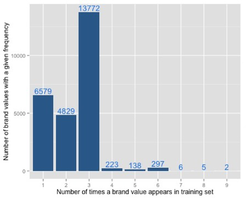
Figure 1: Distribution of label frequencies in the training set

Given the large number of classes and since over 95% of labels appear 3 times or less in the training set, there is very little training data per class to train an effective model using text classification techniques.

To obtain the nearest neighbors benchmarks, we used a bag of words model where each token was encoded using its tf-idf score and the nearest neighbors were obtained using cosine similarity. Given the frequency of labels shown above, we compare our results to those of k nearest neighbors models with k equal to 1 (1NN) and 3 (3NN). For 3NN, in case all three closest neighbors corresponded to distinct labels, the label with the highest cosine similarity was chosen i.e. the result would coincide with that of 1NN in this case. All results were obtained using a 10-fold cross validation.

Note that since some labels appear only once, if such a label occurs in the test set during cross validation, both 1NN and 3NN would be incapable of producing the correct result. However, considering one of the goals of the attribute extraction system is to discover new attribute values, this situation closely models the reality of the data.

9.2.2 Dictionary based approaches

For dictionary based benchmarks, we compile a lexicon of brands that appear in the training data with some preprocessing (lowercasing and tokenization). Given a test title, we perform the same preprocessing and we search for the presence of any brand from the lexicon in the title. We show the results from two approaches that were obtained from the heuristic used to resolve multiple matches:

1. Dict-max: In case of multiple matches, we choose the match with the largest number of characters.

2. Dict-first: In case of multiple matches, we choose the match that appears earliest in the title.

9.2.3 Hidden Markov Model

For an input sequence $\mathbf{x}=x_{1},x_{2},...,x_{m}$, and a label sequence $\mathbf{y}=y_{1},y_{2},...,y_{m}$, a second-order Hidden Markov Model (HMM) defines the joint probability of the input and label sequences as follows

$$\text{Pr}(x_{1},x_{2},...,x_{m},y_{1},y_{2},...,y_{m})$$

$$=\Pi_{i=1}^{m+1}\text{Pr}(y_{i}|y_{i-2},y_{i-1})\Pi_{i=1}^{m}\text{Pr}(x_{i}|y_{i})$$

where $y_{-1},y_{0}=\text{START}$ and $y_{m+1}=\text{STOP}$ are special labels. The probabilities on the right hand side of the above equation are parameters of the HMM and can be estimated from a training set of input and label sequences using maximum likelihood estimation. Given a test sequence, the label sequence that maximizes the above joint probability is chosen.

In estimating probabilities for unknown words, we mapped them to one of several morphological classes similar to [2].

9.2.4 Model comparisons

The results for all models are shown below. The error margins indicate two standard errors.

	Precision (%)	Recall (%)	Label Accuracy (%)
LCCRF	91.94$\pm$0.25	92.21$\pm$0.25	98.44$\pm$0.04
SP	91.98$\pm$0.21	92.18$\pm$0.22	98.44$\pm$0.03
HMM	79.73$\pm$0.28	86.13$\pm$0.26	92.41$\pm$0.09
Dict-max	80.91$\pm$0.42	77.66$\pm$0.45	NA
Dict-first	79.46$\pm$0.36	76.27$\pm$0.41	NA
1NN	69.77$\pm$0.43	69.66$\pm$0.46	NA
3NN	65.88$\pm$0.62	65.75$\pm$0.64	NA

Table 1: Model metrics for brand extraction

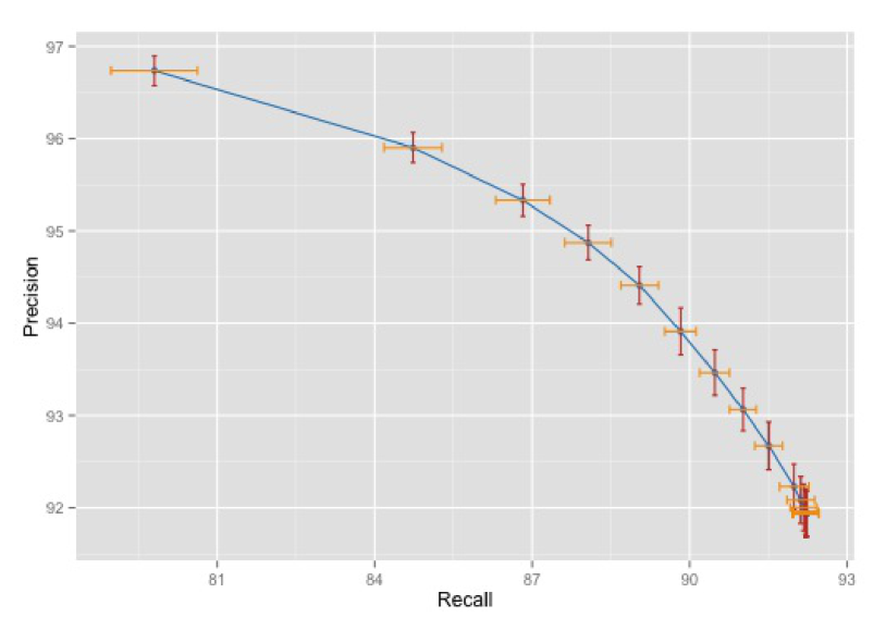
Figure 2: Precision vs Recall for LCCRF model for brand extraction (the error bars indicate two standard errors)

LCCRF and SP outperform the rest of the models and yield similar performance. The metrics for these models also meet business specifications at Walmart to power algorithmic solutions to extract product metdata.

The high label accuracy compared to the precision of the algorithm indicates a crucial fact that we exploited for post processing. In a large number of cases even when the predicted sequence labeling was incorrect, almost all the tokens still had the right label. What we observed was that the false positive brand value predictions typically were either subsequences or supersequences of the expected unnormalized brand. Due to this, we were able to employ the normalization scheme to improve both precision and recall further.

We will illustrate this with an example. Consider the following product title

Plum Island Silver SC-007 Sterling Silver Fairy Piece Ear Cuff

that contains the brand name ‘Plum Island Silver’. Suppose the sequence labeling algorithm incorrectly extracts the brand value as ‘Plum Island’. In such a case, we add the pair (‘Plum Island’, ‘Plum Island Silver’) to the normalization dictionary while adding the above title in the training set with the correctly annotated brand. In a subsequent run, it’s highly likely that either the algorithm adapts and correctly predicts the brand or still returns the previous truncated value. However, even in the latter case, the normalization scheme will correctly pick the desired normalized value.

10 Other attributes

The system is easily extended to a number of other attributes where we may not have a pre compiled list of possible attribute values or when such a list is large and may undergo frequent changes. Some examples include manufacturer specific model numbers and names, fictional characters that inspire children’s toys, sports team and league names for sports branded apparel and memorabilia, product lines, etc. The approach presented above is readily amenable for the extraction of such attributes. Most of the methodology remains similar to that used for brands. We were able to use the same algorithms, similar set of features, distant supervision to produce annotated product titles for training and normalization schemes for standardization of variations of attributes values to build models with high precision and recall for such attributes.

11 Real world performance

We used the approach presented above to extract brands for a subset of products in selected departments. Early results from algorithmic extraction were manually validated by analysts. The normalization dictionary was regularly updated based on analyst feedback. For the manually validated batches, post normalization precision varied between 92%-95% showing an improvement between 1%-3% over algorithmically extracted values. Sample validations of the products categorized as unbranded revealed that over 98% of those were indeed true negatives. The algorithm was able to ‘discover’ over a thousand brand values which were not part of the Walmart brand database at that point.

We estimated the impact of brand value extraction on product discoverability using the R package CausalImpact [4]. For the following analysis, the brand attribute value was extracted and used to augment product data for 272,697 products on the same day. We measured the impressions for this set of products during 44 days prior and 27 days following this intervention conditioned on the brand facet being applied. The results of the analysis are shown below.

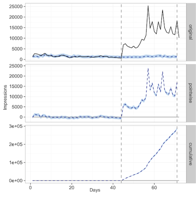
Figure 3: Daily impressions for products for which brand attribute value was extraced

The plot consists of three panels. The solid line in the top panel shows the actual daily impressions for the set of products. The first vertical dotted line indicates the day of intervention (products augmented with brand metadata). The second vertical line marks the end of the measurement. The blue dotted time series in the first panel is the predicted counterfactual - how the impressions would have tracked in the absence of the intervention. The second panel shows the difference between the observed impressions and the counterfactual predictions while the final plot shows the cumulative difference. The synthetical control was constructed from products from similar categories for which no brand metadata was augmented. The model predicts over 250K additional impressions during the test period for the set of items for which the brand metadata was supplied. Similar analysis for other attributes for which attribute extraction was employed typically suggests a positive impact on impressions and depending on the attribute also on other metrics of interest such as clicks, add to cart rate and orders.

So far, the attribute extraction system has been deployed for extracting over 20 attributes. We build a separate model for each attribute for several reasons. A given attribute is typically applicable to only a particular set of categories (for e.g. brand may not be an important attribute for books while sports team may not be applicable for electronic tablet devices). Building a separate model for each attribute allows us to independently train each model and tune the performance based on business needs. The size of the training set varies between a few hundred titles to tens of thousands depending on the attribute.

12 Conclusion

In this paper, we introduced the problem of extracting attribute values from product titles in order to augment product metdata for eCommerce catalogs. We discussed the importance of attribute extraction for retail websites. We examined the challenges associated with this task especially when the product catalog is large. Attribute extraction from product titles was modeled as a sequence labeling problem. We also illustrated a method to leverage existing products tagged with attribute values to build the initial training data set without manual labeling. The experimental results show that SP or LCCRF models combined with a curated normalization scheme provide an efficacious mechanism for tagging products with certain attribute values with high precision and recall.

References

- [1] Harith Alani, Sanghee Kim, David E. Millard, Mark J. Weal, Wendy Hall, Paul H. Lewis, and Nigel R. Shadbolt. Automatic ontology-based knowledge extraction from web documents. IEEE Intelligent Systems, 18(1):14–21, 2003.
- [2] Daniel M. Bikel, Richard Schwartz, and Ralph M. Weischedel. An algorithm that learns what’s in a name. Machine Learning, 34(1–3):211–231, February 1999.
- [3] Eric Brill. A simple rule-based part of speech tagger. Proceedings of the Third Conference on Applied Natural Language Processing, pages 152–155, 1992.
- [4] Kay H Brodersen, Fabian Gallusser, Jim Koehler, Nicolas Remy, Steven L Scott, et al. Inferring causal impact using bayesian structural time-series models. The Annals of Applied Statistics, 9(1):247–274, 2015.
- [5] Laura Chiticariu, Rajasekar Krishnamurthy, Yunyao Li, Frederick Reiss, and Shivakumar Vaithyanathan. Domain adaptation of rule-based annotators for named-entity recognition tasks. In Proceedings of the 2010 Conference on Empirical Methods in Natural Language Processing, pages 1002–1012, 2010.
- [6] Michael Collins. Discriminative training methods for hidden markov models: Theory and experiments with perceptron algorithms. Proceedings of the 2002 Conference on Empirical Methods in Natural Language Processing, 10:1–8, 2002.
- [7] Oren Etzioni, Michael Cafarella, Doug Downey, Ana-Maria Popescu, Tal Shaked, Stephen Soderland, Daniel S. Weld, and Alexander Yates. Unsupervised named-entity extraction from the web: An experimental study. Artificial Intelligence, 165(1):91–134, 2005.
- [8] Dimitra Farmakiotou, Vangelis Karkaletsis, John Koutsias, George Sigletos, Constantine D Spyropoulos, and Panagiotis Stamatopoulos. Rule-based named entity recognition for greek financial texts. In Proceedings of the Workshop on Computational lexicography and Multimedia Dictionaries (COMLEX 2000), pages 75–78, 2000.
- [9] R. Ghani, K. Probst, Y. Liu, M. Krema, and A. Fano. Text mining for product attribute extraction. SIGKDD, 8(1):41–48, 2006.
- [10] Yoav Goldberg and Michael Elhadad. Learning sparser perceptron models. Technical report, Ben Gurion University of the Negev, 2011.
- [11] Anitha Kannan, Patha Talukdar, Nikhil Rasiwasia, and Qifa Ke. Improving product classification using images. Data Mining (ICDM), 2011 IEEE 11th International Conference on, pages 310–319, 2011.
- [12] Jun’ichi Kazama and Kentaro Torisawa. Exploiting wikipedia as external knowledge for named entity recognition. Proceedings of the 2007 Joint Conference on Empirical Methods in Natural Language Processing and Computational Natural Language Learning, pages 698–707, 2007.
- [13] J. Lafferty, A. McCallum, and F. Pereira. Conditional random fields: probabilistic models for segmenting and labeling sequence data. International Conference on Machine Learning, 2001.
- [14] Mitchell P Marcus and Mary Ann Marcinkiewicz. Building a large annotated corpus of english: The penn treebank. Computational Linguistics, 19(2), 1993.
- [15] Andrei Mikheev, Marc Moens, and Clair Grover. Named entity recognition without gazetteers. In Proceedings of the ninth conference on European chapter of the Association for Computational Linguistics, pages 1–8. Association for Computational Linguistics, 1999.
- [16] David Nadeau and Satoshi Sekine. A survey of named entity recognition and classification. Lingvisticae Investigationes, 30(1):3–26, 2007.
- [17] Ana-Maria Popescu and Oren Etzioni. Extracting product features and opinions from reviews. Natural language processing and text mining, pages 9–28, 2007.
- [18] Duangmanee Putthividhya and Junling Hu. Bootstrapped named entity recognition for product attribute extraction. Proceedings of the 2011 Conference on Empirical Methods in Natural Language Processing, pages 1557–1567, 2011.
- [19] Alan Ritter, Sam Clark, Mausam, and Oren Etzioni. Named entity recognition in tweets: An experimental study. Proceedings of the Conference on Empirical Methods in Natural Language Processing, pages 1524–1534, 2011.
- [20] Helmut Schmid. Probabilistic part-of-speech tagging using decision trees. Proceedings of the international conference on new methods in language processing, 12:44–49, 1994.
- [21] Maksim Tkachenko and Andrey Simanovsky. Named entity recognition: Exploring features. In Proceedings of KONVENS, pages 118–127, 2012.