Coherent observations of gravitational radiation
with LISA and gLISA

Abstract

The geosynchronous Laser Interferometer Space Antenna (gLISA) is a space-based gravitational wave (GW) mission that, for the past five years, has been under joint study at the Jet Propulsion Laboratory, Stanford University, the National Institute for Space Research (I.N.P.E., Brazil), and Space Systems Loral. If flown at the same time as the LISA mission, the two arrays will deliver a joint sensitivity that accounts for the best performance of both missions in their respective parts of the milliHertz band. This simultaneous operation will result in an optimally combined sensitivity curve that is “white” from about $3\times 10^{-3}\ {\rm Hz}$ to $1\ {\rm Hz}$, making the two antennas capable of detecting, with high signal-to-noise ratios (SNRs), coalescing black-hole binaries (BHBs) with masses in the range $(10-10^{8})M_{\odot}$. Their ability of jointly tracking, with enhanced SNR, signals similar to that observed by the Advanced Laser Interferometer Gravitational Wave Observatory (aLIGO) on September 14, 2015 (the GW150914 event) will result in a larger number of observable small-mass binary black-holes and an improved precision of the parameters characterizing these sources. Together, LISA, gLISA and aLIGO will cover, with good sensitivity, the $(10^{-4}-10^{3})\ {\rm Hz}$ frequency band.

The first direct observation of a GW signal announced by the LIGO project LIGO on February 11, 2016 GW150914 , represents one of the most important achievements in experimental physics today, and marks the beginning of GW astronomy Thorne1987 . By simultaneously measuring and recording strain data with two interferometers at Hanford (Washington) and Livingston (Louisiana), scientists were able to reach an extremely high level of detection confidence and infer unequivocally the GW source of the observed signal to be a coalescing binary system containing two black-holes of masses $M_{1}=36^{+5}_{-4}\ M_{\odot}$ and $M_{2}=29^{+4}_{-4}\ M_{\odot}$ out to a luminosity distance of $410^{+160}_{-180}\ Mpc$ corresponding to a red-shift $z=0.09^{+0.03}_{-0.04}$ (the above uncertainties being at the $90$ percent confidence level). The network of the two LIGO interferometers could constrain the direction to the binary system only to a broad region of the sky because the French-Italian VIRGO detector VIRGO was not operational at the time of the detection and no electromagnetic counterparts could be uniquely associated with the observed signal.

Ground-based observations inherently require use of multiple detectors widely separated on Earth and operating in coincidence. This is because a network of GW interferometers operating at the same time can (i) very effectively discriminate a GW signal from random noise and (ii) provide enough information for reconstructing the parameters characterizing the wave’s astrophysical source (such as its sky-location, luminosity distance, mass(es), dynamical time scale, etc.) SchutzTinto ; GT . Space-based interferometers instead, with their six links along their three-arms, have enough data redundancy to validate their measurements and uniquely reconstruct an observed signal PPA1998 . A mission such as LISA, with its three operating arms, will be able to assess its measurements’ noise level and statistical properties over its entire observational frequency band. By relying on a time-delay interferometric (TDI) measurement that is insensitive to gravitational waves TAE , LISA will assess its in-flight noise characteristics in the lower part of the band, i.e. at frequencies smaller than the inverse of the round-trip-light time. At higher frequencies instead, where it can synthesize three independent interferometric measurements, it will be able to perform a data consistency test by relying on the null-stream technique GT ; TL ; SST , i.e. a parametric non-linear combination of the TDI measurements that achieves a pronounced minimum at a unique point in the search parameter space when a signal is present. In addition, by taking advantage of the Doppler and amplitude modulations introduced by the motion of the array around the Sun on long-lived GW signals, LISA will measure the values of the parameters associated with the GW source of the observed signal PPA1998 .

Although a single space-based array such as LISA can synthesize the equivalent of four interferometric (TDI) combinations (such as the Sagnac TDI combinations $(\alpha,\beta,\gamma,\zeta)$) TD2014 , its best sensitivity level is achieved only over a relatively narrow region of the mHz frequency band. At frequencies lower than the inverse of the round-trip light time, the sensitivity of a space-based GW interferometer is determined by the level of residual acceleration noise associated with the nearly free-floating proof-masses of the onboard gravitational reference sensor and the size of the arm-length. This is because in this region of the accessible frequency band the magnitude of a gravitational wave signal in the interferometer’s data scales linearly with the arm-length. At frequencies higher than the inverse of the round-trip light time instead, the sensitivity is primarily determined by the photon-counting statistics TAAA . Note that this noise grows linearly with the arm-length through its inverse proportionality to the square-root of the received optical power and because, in this region of the accessible frequency band, the gravitational wave signal no-longer scales with the arm-length. In summary, for a given performance of the onboard science instrument and optical configuration, the best sensitivity level and the corresponding wideness of the bandwidth over which it is reached are uniquely determined by the size of the array.

The best sensitivity level and the corresponding bandwidth over which it is reached by a space-based interferometer become particularly important when considering signals sweeping up-wards in frequency such as those emitted by coalescing binary systems containing black-holes. As recently pointed out by Sesana Sesana , it is theoretically expected that a very large ensemble of coalescing binary systems, with masses comparable to those of GW150914, will have characteristic wave’s amplitudes that could be observable by LISA over an accessible frequency region from about $1.5\times 10^{-2}$ Hz to about $7.6\times 10^{-2}$ Hz. These frequency limits correspond to (i) the assumption of observing a GW150914-like signal for a period of five years (approximately equal to its coalescing time), and (ii) the value at which the signal’s amplitude is equal to the LISA sensitivity. Although one could in principle increase the size of the LISA’s optical telescopes and rely on more powerful lasers so as to increase the upper frequency cut-off to enlarge the observational bandwidth, in practice pointing accuracy and stability requirements together with the finiteness of the onboard available power would result in a negligible gain.

A natural way to broaden the mHz band, so as to fill the gap between the region accessible by LISA and that by the ground interferometers, is to simultaneously fly an additional interferometer with a smaller arm-length. The geosynchronous Laser Interferometer Space Antenna (gLISA) TAAA ; TBDT ; TAKAA , which has been analyzed during the past five years by a collaboration of scientists and engineers at the Jet Propulsion Laboratory, Stanford University, the National Institute for Space Research (I.N.P.E., Brazil), and Space Systems Loral, would allow this footnote1 . With an arm-length of about $7.3\times 10^{4}$ km, it could achieve a shot-noise limited sensitivity in the higher region of its accessible frequency band that is about a factor of $70$ better than that of LISA footnote2 ; gLISA will display a minimum of its sensitivity in a frequency region that perfectly complements those of LISA and aLIGO, resulting into an overall accessible GW frequency band equal to $(10^{-4}-10^{3})\ {\rm Hz}$.

To derive the expression of the joint LISA-gLISA sensitivity, we first note that the noises in the TDI measurements made by the two arrays will be independent. This means that the joint signal-to-noise ratio squared, averaged over an ensemble of signals randomly distributed over the celestial sphere and random polarization states, $\langle SNR_{eL+gL}^{2}\rangle$, can be written in the following form

$$\langle SNR_{eL+gL}^{2}\rangle \equiv 4\int_{f_{1}}^{f_{2}}\frac{|{\widetilde{h}}(f)|^{2}}{S_{h}^{eL+gL}(f)}\ df\ =\langle SNR_{eL}^{2}\rangle+\langle SNR_{gL}^{2}\rangle$$ (1)

$$= 4\int_{f_{1}}^{f_{2}}\left\{\frac{1}{S_{h}^{eL}(f)}+\frac{1}{S_{h}^{gL}(f)}\right\}|{\widetilde{h}}(f)|^{2}\ df\ ,$$

where the functions $S_{h}^{i}(f),\ i=eL\ ,\ gL$ correspond to the squared optimal sensitivities (as defined through the $A$, $E$, and $T$ modes PTLA ; TD2014 ) of the LISA and gLISA arrays respectively. Note that the factor $4$ in front of the integral in Eq.(1) reflects the adopted convention throughout this article of using one-sided power spectral densities of the noises FH1998 ; TA .

From Eq. (1) it is straightforward to derive the following expression of the joint sensitivity squared, $S_{h}^{eL+gL}(f)$, in terms of the individual ones, $S_{h}^{eL}(f)$ and $S_{h}^{gL}(f)$

$$S_{h}^{eL+gL}(f)\equiv\frac{S_{h}^{eL}(f)\ S_{h}^{gL}(f)}{S_{h}^{eL}(f)+S_{h}^{gL}(f)}\ .$$ (2)

In Fig. 1 we plot the optimal sensitivities of LISA (blue), gLISA (red) averaged over sources randomly distributed over the sky and polarization states, together with the joint LISA-gLISA (black) given by Eq. (2). For completeness, and to visually exemplify the scientific advantages of flying simultaneously two space-based missions of different arm-lengths, we have included the anticipated sensitivity of the third-generation aLIGO detector (green) together with the amplitude of the gravitational wave signal GW150914 (magenta) as functions of the Fourier frequency $f$. We have also included a black horizontal line showing the frequency evolution of GW150914 over a 5 years period before coalescence.

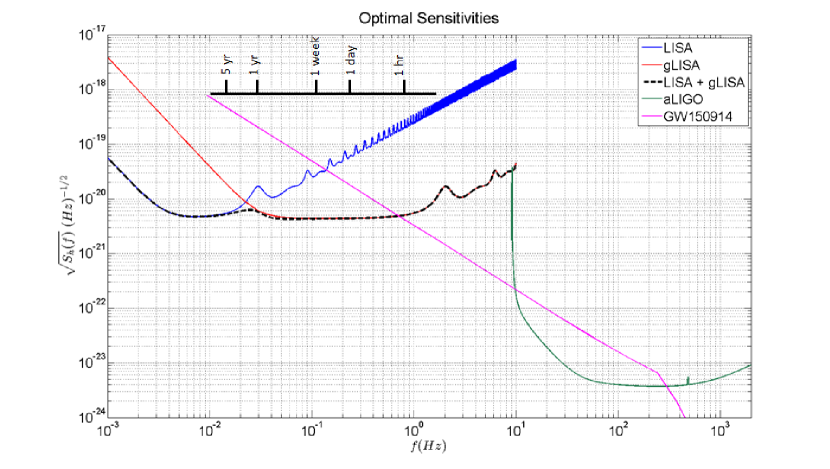
Figure 1: The optimal sensitivities of LISA (blue) and gLISA (red) averaged over sources randomly distributed over the sky and polarization states. Each of these curves is uniquely determined by the TDI $A$, $E$, and $T$ combinations associated with the data from each mission. (see PTLA for the derivation of the $A$, $E$, and $T$ modes and the resulting optimal sensitivity. Also refer to TD2014 for the revised expressions of their noise spectra). The dashed-line (black) is the result of optimally combining the sensitivities of LISA and gLISA. As expected, in the lower part of the mHz band, LISA defines the network sensitivity; in the overlapping region the two sensitivities smoothly blend, resulting in a maximum sensitivity gain of $\sqrt{2}$. In the higher part of the accessible band gLISA defines the joint LISA-gLISA sensitivity. For completeness we have included the projected aLIGO sensitivity (green) together with the amplitude of GW150914 (magenta) as a function of the Fourier frequency $f$. Also included is a black horizontal line showing the frequency evolution of GW150914 over a 5 years period before coalescence.

Shortly before the announcement made by aLIGO of the detection of a second signal emitted by another black-hole binary system, GW151226, with masses roughly half of those of GW150914 GW150914 ; GW151226 , Sesana estimated that a large number of such systems Sesana could be observed by LISA while they are still spiraling around each other over periods as long as the entire five years duration of the mission. Because of these compelling astrophysical reasons, to quantify the scientific advantages of flying gLISA jointly with LISA we will focus our attention on signals emitted by coalescing black-hole binaries with chirp masses in the range $(10-100)M_{\odot}$.

In our analysis we will use the following expressions (valid for circular orbits) of the Fourier transform of the amplitude of the gravitational wave signal emitted by such systems, $\widetilde{h}(f)$, and the time, $t_{c}$, it takes them to coalesce Maggiore

$$\widetilde{h}(f) = \sqrt{\frac{5}{24}}\ \pi^{-2/3}\ \left[\frac{(1+z)GM_{c}}{c^{3}}\right]^{5/6}\ \frac{c}{D_{L}}\ f^{-7/6}\ ,$$ (3)

$$t_{c} = \frac{5}{256}\ \left[\frac{(1+z)GM_{c}}{c^{3}}\right]^{-5/3}\ (\pi f_{gw})^{-8/3}\ .$$ (4)

In Eqs.(3, 4) $G$ is the gravitational constant, $c$ is the speed of light, $z$ is the cosmological red-shift, $D_{L}$ is the corresponding luminosity distance, $M_{c}\equiv(M_{1}M_{2})^{3/5}/(M_{1}+M_{2})^{1/5}$ is the chirp mass associated with the binary system whose components have masses $M_{1}$ and $M_{2}$, $f$ is the Fourier frequency and $f_{gw}$ the instantaneous frequency of the emitted GW.

By using the above signal amplitude and time to coalescence, and by further assuming an integration time of $5$ years (which, in the case of the GW150914 signal, defines the lower-limit of integration in the integral of the SNR to be equal to $0.0151$ Hz), we have estimated the SNRs achievable by the two interferometers when operating either as stand-alone or jointly. We find LISA can observe a GW150914-like signal with a SNR equal to $10.7$, while gLISA with an SNR of $14.4$ because of its better sensitivity over a larger part of its observable band (see Fig. 1). As expected, the joint LISA-gLISA network further improves upon the SNR of gLISA-alone by reaching a value of about $18.0$. From these results we can further infer that gLISA will achieve a sufficiently high SNR to warrant the detection of a GW150914-like signal by integrating for a shorter time. We find that, by integrating for a period of $135$ days prior to the moment of coalesce of a GW150914-like system, gLISA can achieve a SNR of $10.7$.

The level of SNR achievable by the LISA-gLISA network over a five-year integration is about $80$ percent higher than that of LISA alone. This implies, from the estimated parameter precisions derived by Sesana Sesana and their dependence on the value of the SNR CF1994 , that the LISA-gLISA network will estimate the parameters associated with the GW source of the observed signal with a precision that is $1.8$ better than that obtainable by LISA alone. It should be said, however, that this is a lower bound on the improved precision by which the parameters can be estimated since it is based only on SNR considerations. As pointed out by McWilliams in an unpublished document McWilliams , the Doppler frequency shift together with the larger diurnal amplitude modulations experienced by the GW signal in the gLISA TDI measurements will further improve the precision of the reconstructed parameters beyond that due to only the enhanced SNR. We will analyze and quantify this point in a follow-up article as this is beyond the scope of this letter.

From the expressions of the SNR and of the Fourier amplitude of the GW signal, $\tilde{h}(f)$ (Eqs. 1, 3), and by fixing the SNR to a specific value for each operational configuration (stand-alone vs. network), it is possible to infer the corresponding average luminosity distance to a BHB in terms of its chirp mass parameter footnote3 . In Fig. 2 we plot the results of this analysis by assuming a SNR of $10$. As expected, the three derived luminosity distances are monotonically increasing functions of the chirp-mass. For chirp-masses in the range $[10-36)\ M_{\odot}$ gLISA can see signals further away than LISA because of its better sensitivity at higher frequencies. Systems with a chirp-mass larger that $36\ M_{\odot}$ instead can be seen by LISA at a larger luminosity distance than that achievable by gLISA alone. Note that the LISA-gLISA network out-performs the stand-alone configurations by as much as $40$ percent for BHBs with chirp-masses in the interval $(30-40)\ M_{\odot}$. This results into a number of observable events that is about $3$ times larger than that detectable by each interferometer alone. Finally, a GW150914-like signal characterized by a chirp mass of $28.1\ M_{\odot}$ can be see by LISA at an average luminosity distance of about $400\ Mpc$, by gLISA out to $600\ Mpc$, and by the LISA-gLISA system out to about $800\ Mpc$.

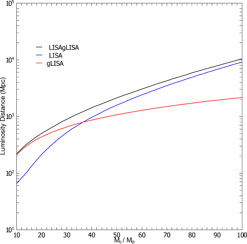
Figure 2: Average luminosity distance achievable by LISA, gLISA and the LISA-gLISA network as function of the chirp mass. The SNR of each configuration has been assumed to be equal to $10$ with an integration time of five years.

In addition to derive the luminosity distance as a function of the chirp-mass (with a chosen value of the SNR), we have also calculated the SNR as a function of the chirp-mass by assuming the SNR of the LISA mission to be constant and equal to $10$ (see Fig. 3). This of course implies that the luminosity distance of the system is uniquely determined by the chirp-mass through the assumed SNR value of $10$ for LISA. Since we are focusing on chirp-masses defined in the interval $[10-100]\ M_{\odot}$, from Fig. 2 we infer that the values assumed by the luminosity distance will be greater than or equal to about $65\$ Mpc. This minimum value of the luminosity distance defines an astrophysical interesting region as it is more than four times larger than the luminosity distance to the Virgo cluster of galaxies.

Fig. 3 shows the two SNRs of gLISA and LISA-gLISA to be decreasing functions of the chirp-mass, with their maximum values of $31$ and $32.5$ respectively at $M_{c}=10\ M_{\odot}$. At $M_{c}\simeq 36\ M_{\odot}$ instead the gLISA SNR also becomes equal to $10$ while, as expected, the LISA-gLISA SNR is $\sqrt{2}$ larger.

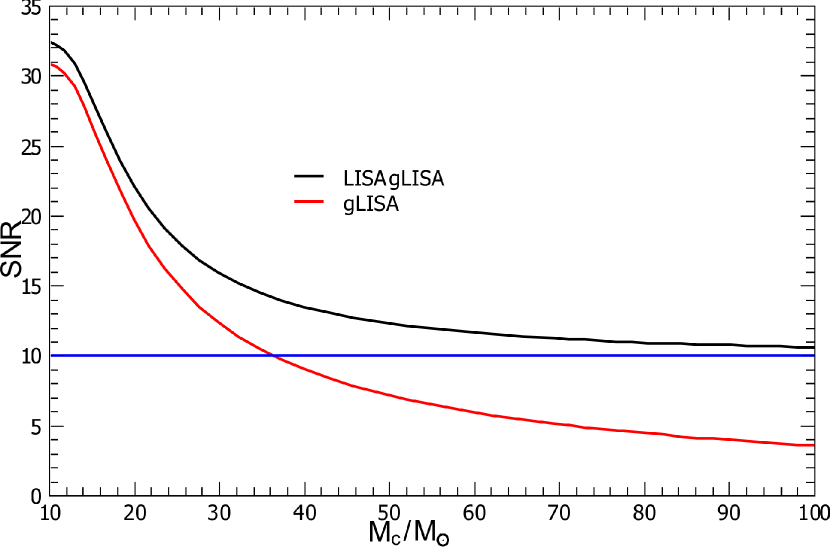
Figure 3: SNR for gLISA and the LISA-gLISA network as a function of the chirp-mass of BHBs that are seen by LISA with an SNR = 10. An integration time of five years is also assumed.

This letter has shown the scientific advantages of simultaneously flying with the LISA mission an additional, smaller size, space-based interferometer such as gLISA. Because of its smaller arm-length, gLISA will be able to survey the region of the GW frequency band that is in between those accessible by LISA and aLIGO. By covering the entire mHz and kHz GW frequency band, LISA, gLISA and aLIGO will detect all known sources emitting in this broad frequency region, and observe signals requiring multi-band detection for understanding the physical nature of their sources.

References

- (1) http://www.ligo.caltech.edu/ .
- (2) B.P. Abbott et al., Phys. Rev. Lett., 116, 061102 (2016).
- (3) K.S. Thorne. In: Three Hundred Years of Gravitation, 330-458, Eds. S.W. Hawking, and W. Israel (Cambridge University Press: New York), (1987).
- (4) http://www.virgo.infn.it/ .
- (5) B.F. Schutz and M. Tinto, M.N.R.A.S., 224, 131 (1987).
- (6) Y. Gürsel and M. Tinto, Phys. Rev. D, 40, 3884, (1989).
- (7) P. Bender, K. Danzmann, & the LISA Study Team, Laser Interferometer Space Antenna for the Detection of Gravitational Waves, Pre-Phase A Report, MPQ233 (Max-Planck- Institüt für Quantenoptik, Garching), July 1998.
- (8) M. Tinto, J.W. Armstrong, and F.B. Estabrook, Phys. Rev. D, 63, 021101(R) (2000).
- (9) M. Tinto and S.L. Larson, Phys. Rev. D, 70, 062002, (2004).
- (10) A.C. Searle, P.J. Sutton, and M. Tinto, Class. Quantum. Grav., 26, 15 (2009).
- (11) M. Tinto and S.V. Dhurandhar, Living Rev. Relativity, 17, 6, (2014).
- (12) M. Tinto, J.C.N. de Araujo, O.D. Aguiar, and M.E.S. Alves, Astroparticle Physics, 48, 50, (2013).
- (13) A. Sesana, Phys. Rev. Lett., 116, 231102 (2016).
- (14) C. Cutler, and E.E. Flanagan, Phys. Rev. D, 49, 2658, (1994).
- (15) M. Tinto, D. DeBra, S. Buchman, and S. Tilley, Review of Scientific Instruments, 86, 014501, (2015).
- (16) M. Tinto, J.C.N. de Araujo, H.K. Kuga, M.E.S. Alves, and O.D. Aguiar, Class. Quantum Grav., 32, 185017, (2015).
- (17) Sean T. McWilliams proposed, independently of us, a mission concept very similar to gLISA called GADFLI. Both concepts were first (independently and simultaneously) proposed to NASA as part of its 2011 Request For Information (RFI) exercise for a LISA-like GW mission RFI .
- (18) The derivation of the gLISA sensitivity and the related discussion on the magnitude of the noises that define it have been presented in the main body and appendix of Ref. TAAA . Although it was stated there that additional technology developments were needed to reduce the optical bench noise level below that of the photon-shot noise, the LISA Pathfinder experiment LPF has demonstrated this noise to be a factor of smaller than its anticipated value.
- (19) NASA solicitation # NNH11ZDA019L titled: “Concepts for the NASA gravitational-wave mission”. http://nspires.nasaprs.com/external/
- (20) M. Armano et al., Phys. Rev. Lett., 116, 231101, (2016).
- (21) T.A. Prince, M. Tinto, S.L. Larson, and J.W. Armstrong, Phys. Rev. D, 66, 122002, (2002).
- (22) E.E. Flanagan and S.A. Hughes, Phys. Rev. D, 57, 4535 (1998).
- (23) M. Tinto and J.W. Armstrong, Phys. Rev. D, 59, 102003 (1999).
- (24) B.P. Abbott, et al., Phys. Rev. Lett., 116, 241103, (2016).
- (25) M. Maggiore, “Gravitational Waves. Volume 1: Theory and Experiments.”(Oxford University Press, Oxford, 2008) First Edition, pag. 174.
- (26) To derive the redshift, , we have assumed a fiducial CDM flat cosmology with the matter density parameter , the cosmological constant density parameter , and the value of the Hubble parameter at the present time . To obtain the luminosity distance, , in terms of the chirp mass, , we have rewritten the SNR as a function of the redshift by expressing in terms of (see Eq. (13) in TAAA ). Then, for a given SNR, we have solved a transcendental equation to obtain z, and from it derived the luminosity distance.
- (27) S.T. McWilliams, http://arxiv.org/abs/1111.3708