HU-EP-16/27

On the logarithmic divergent part of entanglement entropy, smooth versus singular regions

Harald Dorn

Institut für Physik und IRIS Adlershof, Humboldt-Universität zu Berlin,
Zum Großen Windkanal 6, D-12489 Berlin, Germany

Abstract

The entanglement entropy for smooth regions $\cal A$ has a logarithmic divergent contribution with a shape dependent coefficient and that for regions with conical singularities an additional $\mbox{log}^{2}$ term. Comparing the coefficient of this extra term, obtained by direct holographic calculation for an infinite cone, with the corresponding limiting case for the shape dependent coefficient for a regularised cone, a mismatch by a factor two has been observed in the literature. We discuss several aspects of this issue. In particular a regularisation of $\cal A$, intrinsically delivered by the holographic picture, is proposed and applied to an example of a compact region with two conical singularities. Finally, the mismatch is removed in all studied regularisations of $\cal A$, if equal scale ratios are chosen for the limiting procedure.

1 Introduction

The entanglement entropy for compact three-dimensional regions $\cal A$ with a smooth boundary $\partial\cal A$ in $(3+1)$-dimensional conformal quantum field theories has UV-divergent contributions. The leading one is quadratic $\propto 1/\epsilon^{2}$ with a coefficient proportional to the area of $\partial\cal A$. The nextleading term is logarithmic $\propto\mbox{log}\epsilon$ with a shape dependent coefficient derived by Solodukhin in [1]. His formula for the holographic evaluation in the case of strong coupling ${\cal N}=4$ SYM and static regions $\cal A$ in $\mathbb{R}^{(3,1)}$ is [1]

$$S({\cal A})=\frac{1}{4G_{N}^{(5)}}\left(\frac{A(\partial{\cal A})}{2\epsilon^{2}}~{}+~{}K~{}\mbox{log}\epsilon~{}+~{}{\cal O}(1)~{}\right)$$ (1)

with

$$K~{}=~{}\frac{1}{8}~{}\int_{\partial{\cal A}}~{}k^{2}~{}\sqrt{\mbox{det}~{}g}~{}d^{2}z~{},$$ (2)

where $G_{N}^{(5)}$ is the 5-dim. Newton constant, $g$ the induced metric on $\partial{\cal A}\subset\mathbb{R}^{(3,1)}$ and $k$ the trace of its second fundamental form. Obviously, the coefficient $K$ becomes divergent if the surface $\partial{\cal A}$ develops singularities. This is in correspondence to the appearance of a $\mbox{log}^{2}\epsilon$ term in the direct holographic calculation for regions $\cal A$ with conical singularities via the Ryu-Takayanagi formula [2, 3]

$$S({\cal A})=\frac{V(\gamma_{\cal A})}{4G_{N}^{(5)}}~{}.$$ (3)

There $V(\gamma_{\cal A})$ denotes the volume of the minimal spatial $3$-dimensional submanifold $\gamma_{\cal A}\subset AdS_{5}$, approaching the boundary $\partial{\cal A}$ on the boundary of $AdS_{5}$.

The calculation of the regularised volume of $\gamma_{\cal A}$ with UV cutoff $r>\epsilon$ and IR cutoff $\rho<l$ for the case, where $\cal A$ is an infinite cone with opening angle $2\Omega$, yields [4, 5, 8]

$$S_{\epsilon,l}~{}=~{}=\frac{1}{4G_{N}^{(5)}}\left(\frac{\pi~{}\mbox{sin}\Omega}{2}\frac{l^{2}}{\epsilon^{2}}~{}-~{}\frac{\pi~{}\mbox{cos}\Omega~{}\mbox{cot}\Omega}{8}~{}\mbox{log}^{2}\frac{\epsilon}{l}~{}+~{}\cal O(\mbox{log}\epsilon)\right)~{}.$$ (4)

The authors of [4, 5] have raised the question of how the coefficient of the above $\mbox{log}^{2}$ term can be obtained out of Solodukhin’s formula and found agreement up to a mismatch by a numerical factor 2. An analog observation in (5+1) dimensions was made in [6]. Furthermore, the mismatch factor 2 was observed also for certain perturbed spheres in even dimensional CFT’s [7].

Let us sketch the line of reasoning in [4, 5] and parameterise $\partial{\cal A}$, the boundary of the cone, by the coordinates $\rho,\varphi$

$$x_{1}=\rho~{}\mbox{sin}\Omega~{}\mbox{cos}\varphi~{},~{}~{}x_{2}=\rho~{}\mbox{sin}\Omega~{}\mbox{sin}\varphi~{},x_{3}=\rho~{}\mbox{cos}\Omega~{}.$$ (5)

Then the trace of the second fundamental form is

$$k~{}=~{}\frac{\mbox{cot}\Omega}{\rho}~{},$$ (6)

and the square root of the induced metric

$$\sqrt{\mbox{det}~{}g}~{}=~{}\rho~{}\mbox{sin}\Omega~{}.$$ (7)

For a sphere of radius $R$ the corresponding quantities are (use spherical coordinates $\vartheta,\varphi$)

$$k_{\mbox{\scriptsize sphere}}~{}=~{}\frac{2}{R}~{},~{}~{}~{}\sqrt{\mbox{det}~{}g_{\mbox{\scriptsize sphere}}}~{}=~{}R^{2}~{}\mbox{sin}\vartheta~{}.$$ (8)

If one regularises the singular geometry at the tip of the cone by fitting a piece of a small sphere, this piece does not contribute to the divergence of $K$ since the dependence on its radius cancels in the integral (2). Therefore we have

$$K~{}=~{}\frac{2\pi}{8}~{}\int_{\rho_{\mbox{\scriptsize min}}}^{l}\mbox{cot}^{2}\Omega~{}\mbox{sin}\Omega~{}\frac{d\rho}{\rho}~{}+~{}{\cal O}(1)~{}=~{}-~{}\frac{\pi~{}\mbox{cos}\Omega~{}\mbox{cot}\Omega}{4}~{}\mbox{log}\frac{\rho_{\mbox{\scriptsize min}}}{l}~{}+~{}{\cal O}(1)~{}.$$ (9)

By the natural identification of $\rho_{\mbox{\scriptsize min}}$ with $\epsilon$ one gets $K\mbox{log}\epsilon=-~{}\frac{\pi~{}\mbox{cos}\Omega~{}\mbox{cot}\Omega}{4}~{}\mbox{log}^{2}\epsilon~{}+~{}\dots$ and the mismatch by a factor of 2 relative to the direct holographic calculation (4) as observed in [4, 5].

At this point it is tempting to suspect IR/UV mixing under conformal transformations for this mismatch. A corresponding argument could start as follows. By the natural choice $l=1/\rho_{\mbox{\scriptsize min}}$ we would arrive at

$$K~{}=~{}-~{}\frac{\pi~{}\mbox{cos}\Omega~{}\mbox{cot}\Omega}{2}~{}\mbox{log}\rho_{\mbox{\scriptsize min}}~{}+~{}{\cal O}(1)~{}.$$ (10)

After $\rho_{\mbox{\scriptsize min}}=\epsilon$ this agrees perfectly with what one gets from the direct calculation (4) after $l=1/\epsilon$ (note: $\mbox{log}^{2}\epsilon^{2}=4\mbox{log}^{2}\epsilon$). However, this is a doubtful reasoning, since it immediately breaks down if one uses the dimensionless quotient $\epsilon/l$ as the argument of the log in eq.(1), too. This again would bring back the factor 2.

What remains from this aside is, that for a clean discussion of the behaviour of Solodukhins formula in the limit of singular boundaries $\partial{\cal A}$, we have to rely on its use for compact regions ${\cal A}$.

2 Coefficient of logarithmic divergence for banana shaped regions with rounded tips

As an example for a compact region ${\cal A}$ with two conical singularities we take a banana shaped region as studied in our paper [8]. In a first attempt, for the regularisation we apply the technique used in the previous section: replacement of the conical tips by suitable fitted parts of small spheres. The boundary $\partial{\cal A}$ is given by

$$x_{1}(\rho,\varphi) = \frac{\rho~{}\mbox{cos}\alpha~{}\mbox{sin}\Omega~{}\mbox{cos}\varphi+\rho~{}\mbox{sin}\alpha~{}\mbox{cos}\Omega}{q^{2}+\rho^{2}+2q\rho~{}\hat{w}(\varphi)}~{},$$

$$x_{2}(\rho,\varphi) = \frac{\rho~{}\mbox{sin}\Omega~{}\mbox{sin}\varphi}{q^{2}+\rho^{2}+2q\rho~{}\hat{w}(\varphi)}~{},$$

$$x_{3}(\rho,\varphi) = \frac{q+\rho~{}\hat{w}(\varphi)}{q^{2}+\rho^{2}+2q\rho~{}\hat{w}(\varphi)}~{},$$ (11)

with $0\leq\rho<\infty,~{}0\leq\varphi<2\pi$ and

$$\hat{w}(\varphi)~{}=~{}\mbox{cos}\alpha~{}\mbox{cos}\Omega-\mbox{sin}\alpha~{}\mbox{sin}\Omega~{}\mbox{cos}\varphi~{}.$$ (12)

$2\Omega$ is the opening angle of the conical tips, $\alpha$ is the angle between its axis and the straight line connecting the tips, $1/q$ is the distance between the tips.

The induced metric on $\partial{\cal A}$ is

$$g_{\rho\rho} = \frac{1}{\big{(}q^{2}+\rho^{2}+2q\rho~{}\hat{w}(\varphi)\big{)}^{2}}~{},~{}~{}~{}g_{\rho\varphi}~{}=~{}0~{},$$

$$g_{\varphi\varphi} = \frac{\rho^{2}~{}\mbox{sin}^{2}\Omega}{\big{(}q^{2}+\rho^{2}+2q\rho~{}\hat{w}(\varphi)\big{)}^{2}}~{}.$$ (13)

The second fundamental form turns out as

$$k_{\rho\rho} = \frac{2q~{}(\mbox{sin}\alpha~{}\mbox{cos}\Omega~{}\mbox{cos}\varphi+\mbox{cos}\alpha~{}\mbox{sin}\Omega)}{\big{(}q^{2}+\rho^{2}+2q\rho~{}\hat{w}(\varphi)\big{)}^{2}}~{},~{}~{}~{}k_{\rho\varphi}~{}=~{}0~{},$$

$$k_{\varphi\varphi} = \frac{\rho~{}\mbox{sin}\Omega~{}\big{(}2q\rho~{}\mbox{cos}\alpha+(q^{2}+\rho^{2})\mbox{cos}\Omega\big{)}}{\big{(}q^{2}+\rho^{2}+2q\rho~{}\hat{w}(\varphi)\big{)}^{2}}~{},$$ (14)

and its trace is

$$k:=g^{mn}k_{mn}=~{}2q(\mbox{sin}\alpha~{}\mbox{cos}\Omega~{}\mbox{cos}\varphi+\mbox{cos}\alpha~{}\mbox{sin}\Omega)~{}+~{}\frac{2q\rho~{}\mbox{cos}\alpha+(q^{2}+\rho^{2})\mbox{cos}\Omega}{\rho~{}\mbox{sin}\Omega}~{}.$$ (15)

The integrand in Solodukhin’s formula (2) behaves for $\rho\rightarrow 0$ as

$$k^{2}~{}\sqrt{\mbox{det}~{}g}~{}=~{}\frac{\mbox{cos}\Omega~{}\mbox{cot}\Omega}{\rho}~{}+~{}{\cal O}(1)$$ (16)

and for $\rho\rightarrow\infty$ as

$$k^{2}~{}\sqrt{\mbox{det}~{}g}~{}=~{}\frac{\mbox{cos}\Omega~{}\mbox{cot}\Omega}{\rho}~{}+~{}{\cal O}(1/\rho^{2})~{}.$$ (17)

As discussed in the previous section, the regularising spherical pieces do not contribute to the divergence. Performing the $\varphi$-integration and cutting the logarithmic divergent $\rho$-integration at $\rho_{\mbox{\scriptsize min}}$ and $\rho_{\mbox{\scriptsize max}}$ we get

$$K~{}=~{}\frac{2\pi}{8}~{}\mbox{cos}\Omega~{}\mbox{cot}\Omega~{}(-\mbox{log}\rho_{\mbox{\scriptsize min}}~{}+~{}\mbox{log}\rho_{\mbox{\scriptsize max}})~{}+~{}\dots~{},$$ (18)

where the dots stands for terms staying finite if one removes the cutoffs. With $\rho_{\mbox{\scriptsize min}}=1/\rho_{\mbox{\scriptsize max}}=\epsilon$ this yields

$$K\mbox{log}\epsilon~{}=~{}-\frac{\pi}{2}~{}\mbox{cos}\Omega~{}\mbox{cot}\Omega~{}\mbox{log}^{2}\epsilon~{}+~{}{\cal O}(\mbox{log}\epsilon)~{}.$$ (19)

Comparing this with our result [8] for the direct holographic calculation in the case of unregularised conical tips, one again gets a mismatch by a factor 2.

From this example we can conclude that the origin of the mismatch is not related to the IR/UV issue. Instead it has to be located in the use of different limiting procedures. In the direct holographic calculation one uses only one cutoff (Poincaré coordinate $r>\epsilon$) for the volume of the minimal submanifold $\gamma_{\cal A}$ related to a region $\cal A$ with conical singularities. On the other side at first the same holographic recipe is applied for a smoothed $\cal A$ obtained by rounding the conical singularities. This rounding introduces further independent regularisation parameters ($\rho_{\mbox{\scriptsize min}},\rho_{\mbox{\scriptsize max}}$). Relating them to $\epsilon$ as above sounds natural but, taken seriously, is an ambiguous procedure. Note also that e.g. $\rho_{\mbox{\scriptsize min}}=1/\rho_{\mbox{\scriptsize max}}=\epsilon^{1/2}$ would remove the unwanted mismatch factor 2. We will come back to this point in the conclusion section.

But before we would like to explore another option, to replace the handmade regularisation of $\partial{\cal A}$ for the use in Solodukhin’s formula (2) by one which is delivered by the holographic recipe itself. Let us consider the minimal submanifold $\gamma_{\cal A}$ needed for the treatment of a singular region $\cal A$. Then for use in (2) we take its intersection with the hyperplane $r=\epsilon$ as our regularised version of $\partial\cal A$. This procedure we will demonstrate in the next section with its application to lemon shaped regions.

3 Coefficient of log$\epsilon$ for lemon shaped regions with a holographically induced regularisation

In [8] the minimal submanifold $\gamma_{\cal A}$ in Euclidean $AdS_{4}$ , whose volume up to the factor $\frac{1}{4G_{N}^{(5)}}$ determines the holographic entanglement entropy of a banana shaped region (11), has been obtained

$$x_{1} = \frac{\rho~{}(\mbox{cos}\alpha~{}\mbox{sin}\vartheta~{}\mbox{cos}\varphi~{}+~{}\mbox{sin}\alpha~{}\mbox{cos}\vartheta)}{q^{2}~{}+~{}\rho^{2}(1+h^{2}(\vartheta))~{}+2q\rho~{}w(\vartheta,\varphi)},$$

$$x_{2} = \frac{\rho~{}\mbox{sin}\vartheta~{}\mbox{sin}\varphi}{q^{2}~{}+~{}\rho^{2}(1+h^{2}(\vartheta))~{}+2q\rho~{}w(\vartheta,\varphi)},$$

$$x_{3} = \frac{q~{}+~{}\rho~{}w(\alpha,\vartheta,\varphi)}{q^{2}~{}+~{}\rho^{2}(1+h^{2}(\vartheta))~{}+2q\rho~{}w(\vartheta,\varphi)},$$

$$r = \frac{\rho~{}h(\vartheta)}{q^{2}~{}+~{}\rho^{2}(1+h^{2}(\vartheta))~{}+2q\rho~{}w(\vartheta,\varphi)}~{},$$ (20)

with $w(\vartheta,\varphi)~{}=~{}\mbox{cos}\alpha~{}\mbox{cos}\vartheta~{}-~{}\mbox{sin}\alpha~{}\mbox{sin}\vartheta~{}\mbox{cos}\varphi$ and $h(\vartheta)$ the solution of the differential equation

$$\big{(}~{}\ddot{h}(h+h^{3})+\dot{h}^{2}(3+h^{2})+3+5h^{2}+2h^{4}~{}\big{)} \mbox{sin}\vartheta$$

$$+~{}h\dot{h}(1+h^{2}+\dot{h}^{2}) \mbox{cos}\vartheta =~{}0~{}$$ (21)

and the boundary condition $h(\Omega)=0,~{}~{}h(0)=h_{0}(\Omega)>0$.

Here $\rho,\vartheta,\varphi$ are coordinates and $q,\Omega,\alpha$ parameters fixing the geometry of the banana shaped region as described in the previous section. The regularised volume of this $\gamma_{\cal A}$ has been calculated up to terms vanishing for $\epsilon\rightarrow 0$. We show here only the $\mbox{log}^{2}\epsilon$ term

$$V_{\epsilon}~{}=~{}\dots~{}-\frac{\pi~{}\mbox{cos}\Omega~{}\mbox{cot}\Omega}{4}~{}\mbox{log}^{2}(q\epsilon)~{}+~{}\dots~{}.$$ (22)

As announced above, for a regularised version of ${\cal A}$ we take the intersection of this submanifold with the hyperplane $r=\epsilon$, see fig.1. Then $\partial{\cal A}_{\mbox{\scriptsize reg}}$ is parameterised by the coordinates $\vartheta$ and $\varphi$ via

$$x_{1} = \frac{\rho_{\epsilon}^{\pm}(\vartheta)~{}\mbox{sin}\vartheta~{}\mbox{cos}\varphi}{q^{2}+(\rho_{\epsilon}^{\pm})^{2}(1+h^{2}(\vartheta))+2q\rho_{\epsilon}^{\pm}~{}\mbox{cos}\vartheta}~{},$$

$$x_{2} = \frac{\rho_{\epsilon}^{\pm}(\vartheta)~{}\mbox{sin}\vartheta~{}\mbox{sin}\varphi}{q^{2}+(\rho_{\epsilon}^{\pm})^{2}(1+h^{2}(\vartheta))+2q\rho_{\epsilon}^{\pm}~{}\mbox{cos}\vartheta}~{},$$

$$x_{3} = \frac{q+\rho_{\epsilon}^{\pm}(\vartheta)~{}\mbox{cos}\vartheta~{}}{q^{2}+(\rho_{\epsilon}^{\pm})^{2}(1+h^{2}(\vartheta))+2q\rho_{\epsilon}^{\pm}~{}\mbox{cos}\vartheta}~{},$$ (23)

where $\rho_{\epsilon}^{\pm}$ are the two roots of the equation $r=\epsilon$, i.e.

$$\rho^{\pm}_{\epsilon}(\vartheta)~{}=~{}\frac{h(\vartheta)-2q\epsilon~{}\mbox{cos}\vartheta\pm\sqrt{(h-2q\epsilon~{}\mbox{cos}\vartheta)^{2}-4\epsilon^{2}q^{2}(1+h^{2})}}{2\epsilon~{}(1+h^{2})}~{}.$$ (24)

Each of these two roots is responsible for the description of a half of the regularised boundary of our lemon shaped region.

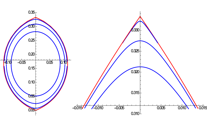
Figure 1: Axial cut of (regularised) lemons=symmetric bananas ($\alpha=0$) with $q=3$.
             In red the original lemons, in blue regularised versions.
On the left: the full picture for $\Omega\approx 1.2$ and $\epsilon=0.02,0.05,0.08~{}.$
On the right: zoom into the upper tip for $\Omega\approx 0.6$ and $\epsilon=0.001,0.005,0.01$.

The induced metric is ($\rho$ stands for $\rho_{\epsilon}^{\pm}(\vartheta)$, $h$ for $h(\vartheta)$ and the dot for $d/d\vartheta$ )

$$g_{\vartheta\vartheta} = \frac{1}{\big{(}q^{2}+2q\rho~{}\mbox{cos}\vartheta+(1+h^{2})\rho^{2}\big{)}^{4}}~{}\Big{\{}\Big{(}\rho\big{(}(-q^{2}+(1+h^{2})\rho^{2})\mbox{sin}\vartheta$$ (25)

$$+2h\dot{h}\rho(q+\rho~{}\mbox{cos}\vartheta)\big{)}+\dot{\rho}\big{(}q^{2}\mbox{cos}\vartheta+\rho(1+h^{2})(2q+\rho~{}\mbox{cos}\vartheta)\big{)}\Big{)}^{2}$$

$$+\Big{(}\rho\big{(}q^{2}\mbox{cos}\vartheta+2q\rho+\rho^{2}((1+h^{2})~{}\mbox{cos}\vartheta-2h\dot{h}~{}\mbox{sin}\vartheta)\big{)}$$

$$+\dot{\rho}\big{(}q^{2}-(1+h^{2})\rho^{2}\big{)}~{}\mbox{sin}\vartheta\Big{)}^{2}\Big{\}}~{},$$

$$g_{\varphi\varphi} = \frac{\rho^{2}~{}\mbox{sin}^{2}\vartheta}{(q^{2}+2q\rho~{}\mbox{cos}\vartheta+(1+h^{2})\rho^{2})^{2}}~{},~{}~{}~{}~{}~{}~{}~{}~{}g_{\vartheta\varphi}~{}=~{}0~{}.$$ (26)

Inserting (24) one gets for the determinant of the induced metric the same expression both for the plus and the minus variant

$$\mbox{det}g(\vartheta) = \frac{\epsilon^{4}\mbox{sin}^{2}\vartheta}{h^{4}\big{(}4\epsilon qh~{}\mbox{cos}\vartheta-(1-4\epsilon^{2}q^{2})h^{2}+4\epsilon^{2}q^{2}\mbox{sin}^{2}\vartheta\big{)}}$$ (27)

$$\cdot\Big{(}4\epsilon qh~{}\mbox{cos}\vartheta-4\epsilon q\dot{h}~{}\mbox{sin}\vartheta-4\epsilon^{2}q^{2}h\dot{h}~{}\mbox{sin}(2\vartheta)$$

$$~{}~{}+2\epsilon^{2}q^{2}(h^{2}-\dot{h}^{2})~{}\mbox{cos}(2\vartheta)-(1-2\epsilon^{2}q^{2})(h^{2}+\dot{h}^{2})\Big{)}~{},$$

which implies for the $\epsilon$-expansion of its square root

$$\sqrt{\mbox{det}g(\vartheta)}~{}=~{}\frac{\mbox{sin}\vartheta~{}\sqrt{h^{2}+\dot{h}^{2}}}{(h(\vartheta))^{3}}~{}\epsilon^{2}~{}+~{}\frac{2q~{}\mbox{sin}\vartheta~{}(h\dot{h}~{}\mbox{sin}\vartheta+\dot{h}^{2}\mbox{cos}\vartheta)}{h^{4}\sqrt{h^{2}+\dot{h}^{2}}}~{}\epsilon^{3}~{}+~{}{\cal O}(\epsilon^{4})~{}.$$ (28)

The trace of the second fundamental form

$$k(\vartheta)=g^{\vartheta\vartheta}~{}\vec{n}~{}\frac{\partial^{2}\vec{x}}{\partial\vartheta^{2}}~{}+~{}g^{\varphi\varphi}~{}\vec{n}~{}\frac{\partial^{2}\vec{x}}{\partial\varphi^{2}}$$ (29)

differs in its plus/minus variant after inserting $\rho_{\epsilon}^{\pm}$ from (24). Expanding the arising longer expressions in $\epsilon$ one gets

$$k^{\pm}(\vartheta)~{}=~{}\frac{h\big{(}2h^{3}+h\dot{h}^{2}\pm\dot{h}^{3}\mbox{cot}\vartheta\pm h^{2}(\dot{h}~{}\mbox{cot}\vartheta+\ddot{h})\big{)}}{(h^{2}+\dot{h}^{2})^{3/2}}~{}\frac{1}{\epsilon}~{}+~{}{\cal O}(1)~{}$$ (30)

and then with (28) for the integrand in Solodukhins formula (2)

$$\sqrt{\mbox{det}g(\vartheta)}~{}(k^{\pm}(\vartheta))^{2}~{}=~{}\frac{\big{(}2h^{3}+h\dot{h}^{2}\pm\dot{h}^{3}\mbox{cot}\vartheta\pm h^{2}(\dot{h}~{}\mbox{cot}\vartheta+\ddot{h})\big{)}^{2}~{}\mbox{sin}\vartheta}{h(h^{2}+\dot{h}^{2})^{5/2}}~{}+~{}{\cal O}(\epsilon)~{}.$$ (31)

From our paper [8] we know for $\vartheta=\Omega-\delta~{},~{}~{}~{}\delta\rightarrow 0$

$$h(\vartheta)~{}=~{}2~{}(\tan\Omega)^{1/2}\delta^{1/2}~{}+~{}{\cal O}(\delta^{3/2}\mbox{log}\delta)~{},$$ (32)

what implies

$$\sqrt{\mbox{det}g}~{}(k^{+})^{2} = \frac{\mbox{cos}\Omega~{}\mbox{cot}\Omega}{2\delta}~{}+~{}\mbox{cos}\Omega+\frac{1}{2}~{}\mbox{cos}\Omega~{}\mbox{cot}^{2}\Omega~{}+~{}{\cal O}(\delta)~{}+~{}{\cal O}(\epsilon)~{},$$ (33)

$$\sqrt{\mbox{det}g}~{}(k^{-})^{2} = \frac{\mbox{cos}\Omega~{}\mbox{cot}\Omega}{2\delta}~{}+~{}5~{}\mbox{cos}\Omega+\frac{1}{2}~{}\mbox{cos}\Omega~{}\mbox{cot}^{2}\Omega~{}+~{}{\cal O}(\delta)~{}+~{}{\cal O}(\epsilon)~{}.$$

The not explicitly shown ${\cal O}(\epsilon)$ terms behave as $\delta^{-3/2}$.

With this estimates we get from (2)

$$K = \frac{1}{8}\int_{0}^{2\pi}d\varphi\int_{0}^{\Omega-\delta_{{\mbox{\scriptsize min}}}}d\vartheta\sqrt{\mbox{det}g(\vartheta)}~{}\big{(}(k^{+}(\vartheta))^{2}+(k^{-}(\vartheta))^{2}\big{)}$$ (34)

$$= \frac{\pi}{4}~{}\frac{\mbox{cos}\Omega~{}\mbox{cot}\Omega}{2}~{}(-2~{}\mbox{log}\delta_{{\mbox{\scriptsize min}}})~{}+~{}{\cal O}(1)~{}+~{}\delta_{{\mbox{\scriptsize min}}}^{-1/2}\cdot{\cal O}(\epsilon)~{}.$$

In the regularisation chosen in this section the upper boundary of the $\vartheta$ integration (lower bd. for $\delta$) is fixed by the vanishing of the expression under the square root in (24). This corresponds to fitting together the two halves of the regularised $\partial{\cal A}$. In this condition $\epsilon\rightarrow 0$ implies $h\rightarrow 0,~{}\vartheta\rightarrow\Omega~{}$. Therefore, with (32) we get

$$\delta_{{\mbox{\scriptsize min}}}~{}=~{}q^{2}\mbox{cot}^{2}\Omega~{}(1+\mbox{cos}\Omega)^{2}~{}\epsilon^{2}~{}+~{}{\cal O}(\epsilon^{3})~{}.$$ (35)

Now we see two facts: At first, due to its singular $\delta^{-3/2}$-behaviour, the integration of the ${\cal O}(\epsilon)$ term of the integrand is not vanishing for $\epsilon\rightarrow 0$, but it does not diverge. At second, due to $\delta_{{\mbox{\scriptsize min}}}\propto\epsilon^{2}$

$$K~{}\mbox{log}\epsilon~{}=~{}-\frac{\pi}{2}~{}\mbox{cos}\Omega~{}\mbox{cot}\Omega~{}\mbox{log}^{2}\epsilon~{}+~{}{\cal O}(\mbox{log}\epsilon)~{}.$$ (36)

This is the same as in the previous section, i.e. the mismatch factor 2 is back.

4 Conclusions

We have found the mismatch factor 2, observed in [4, 5] for the infinite cone, also for prototypical compact regions with two conical singularities. It appeared in section 2 using for Solodukhin’s formula a handmade regularisation of $\partial{\cal A}$, independent of the holographic cut-off procedure. And it reappeared in section 3 using a regularisation of $\partial{\cal A}$, delivered in a natural way by the holographic cut-off procedure itself.

Due to this robustness it is time to answer the question of why this mismatch factor in the so far presented calculations is always just equal to 2.

The direct holographic calculation for $\partial{\cal A}$ depends on one cut-off parameter $\epsilon\rightarrow 0$. We compare it with $\epsilon\rightarrow 0$ for regularised $\partial{\cal A}$ and the subsequent limit of removal of the $\partial{\cal A}$-regularisation. As usual a priori it is open, whether the two different limits yield the same result.

Let us denote by $\epsilon^{\prime}$ the parameter controlling the regularisation of $\partial{\cal A}$. In section 2 we had $\epsilon^{\prime}=\rho_{\mbox{\scriptsize min}}$. In section 3 we used the intersection of the minimal submanifold $\gamma_{\cal A}$ with the $AdS$-hyperplane $r=\epsilon$, but we could have done it also with another hyperplane $r=\epsilon^{\prime}$. Then the universal result for both types of regularisation for $\partial{\cal A}$ is

$$K(\epsilon^{\prime})~{}\mbox{log}\epsilon~{}=~{}-\frac{\pi}{2}~{}\mbox{cos}\Omega~{}\mbox{cot}\Omega~{}\mbox{log}\epsilon^{\prime}~{}\mbox{log}\epsilon~{}+~{}\dots~{}.$$ (37)

Instead of putting $\epsilon^{\prime}=\epsilon$ we better should require that $\epsilon$ goes faster to zero than $\epsilon^{\prime}$. Only in this manner we can keep contact with the appropriate order of limits,

$$\mbox{first}~{}~{}~{}\epsilon\rightarrow 0~{},~{}~{}\mbox{subsequently}~{}~{}~{}\epsilon^{\prime}\rightarrow 0~{}.$$ (38)

Then with $\epsilon^{\prime}=\epsilon^{\beta}~{},~{}~{}0<\beta<1$ we get

$$K~{}\mbox{log}\epsilon~{}=~{}-\beta~{}\frac{\pi}{2}~{}\mbox{cos}\Omega~{}\mbox{cot}\Omega~{}\mbox{log}^{2}\epsilon~{}+~{}\dots~{}.$$ (39)

The choice $\beta=1/2$ yields complete agreement with the direct holographic calculation in [8].

Instead stopping at this point with an ambiguity parametrised by the factor $\beta$, one should stress that $\beta=1/2$ is distinguished not only by the a posteriori fit to the direct calculation. Remarkably, it also corresponds just to the choice of equal scale ratios to mimic the order of limits (38) in a one parameter set up :$~{}~{}\epsilon^{\prime}/1=\epsilon/\epsilon^{\prime}~{}$, i.e. the ratio of the scale for regularising the conical singularity to a constant equals the ratio of the scale for approaching the $AdS$ boundary to the scale for regularising the cone.

Altogether the outcome of our study can be summarised as follows. Based on a naive identification of the two regularisation scales ($\epsilon=\epsilon^{\prime}$), the comparison of the factor for the logarithmic divergence, given by Solodukhin’s formula, in the limit where $\partial{\cal A}$ develops a conical singularity with the direct holographic calculation for the singular $\partial{\cal A}$ yields agreement up to a numerical mismatch factor of 2 [4, 5, 6, 7]. In general the results of different limiting procedures can disagree. Therefore, the fact that in the case under discussion the geometrical structures on both sides are the same, and the only discrepancy is a numerical factor, is already a remarkable result. We have shown that this mismatch factor 2 is robust with respect to the choice of regularisations and, treating compact regions, has nothing to do with the infrared issue for infinite cones. Furthermore, we pinned down the value of the numerical mismatch factor to the implementation of the order of limits (38) in the relation of $\epsilon$ to $\epsilon^{\prime}$. This order is a constitutive ingredient of the path via Solodukhin’s formula (2). Given the universal formula (37), an absence of the mismatch factor for the naive choice would be even confusing, since $\epsilon=\epsilon^{\prime}$ in no respect makes contact with the order of limits (38). The most natural way to mimic this order is realised by the equal scale ratio, i.e. $\beta=1/2$. Then the absence of any mismatch is a consequence.

References

• [1] S.Ā N.Ā Solodukhin, Phys.Ā Lett.Ā B 665 (2008) 305 [arXiv:0802.3117 [hep-th]].
• [2] S.Ā Ryu and T.Ā Takayanagi, Phys.Ā Rev.Ā Lett.Ā  96 (2006) 181602 [hep-th/0603001].
• [3] S.Ā Ryu and T.Ā Takayanagi, JHEP 0608 (2006) 045 [hep-th/0605073].
• [4] I.Ā R.Ā Klebanov, T.Ā Nishioka, S.Ā S.Ā Pufu and B.Ā R.Ā Safdi, JHEP 1207 (2012) 001 [arXiv:1204.4160 [hep-th]].
• [5] R.Ā C.Ā Myers and A.Ā Singh, JHEP 1209 (2012) 013 [arXiv:1206.5225 [hep-th]].
• [6] B.Ā R.Ā Safdi, JHEP 1212 (2012) 005 [arXiv:1206.5025 [hep-th]].
• [7] P.Ā Bueno and R.Ā C.Ā Myers, JHEP 1512 (2015) 168 [arXiv:1508.00587 [hep-th]].
• [8] H.Ā Dorn, JHEP 1606 (2016) 052 [arXiv:1602.06756 [hep-th]].