Abstract

The real parts of the complex squared energies defined by the resonance poles of the transfer matrix of the Pöschl-Teller barrier, are shown to equal the squared energies of the levels bound within the trigonometric Scarf well potential. By transforming these potentials into parts of the Laplacians describing free quantum motions on the mutually orthogonal open time-like hyperbolic–, and closed space-like spherical geodesics on the conformally invariant de Sitter space time, $dS_{4}$, the conformal symmetries of these interactions are revealed. On $dS_{4}$ the potentials under consideration naturally relate to interactions within colorless two-body systems and to cusped Wilson loops. In effect, with the aid of the $dS_{4}$ space-time as unifying geometry, a conformal symmetry based bijective correspondence (duality) between bound and resonant meson spectra is established at the quantum mechanics level and related to confinement understood as color charge neutrality. The correspondence allows to link the interpretation of mesons as resonance poles of a scattering matrix with their complementary description as states bound by an instantaneous quark interaction and to introduce a conformal symmetry based classification scheme of mesons. As examples representative of such a duality we organize in good agreement with data 71 of the reported light flavor mesons with masses below $\sim$ 2350 MeV into four-conformal families of particles placed on linear $f_{0}$, $\pi$, $\eta$, and $a_{0}$ resonance trajectories, plotted on the $\ell/M$ plane. Upon extending the $\sec^{2}\chi$ by a properly constructed conformal color dipole potential, shaped after a tangent function, we predict the masses of 12 “missing” mesons. We furthermore notice that the $f_{0}$ and $\pi$ trajectories can be viewed as chiral partners, same as the $\eta$ and $a_{0}$ trajectories, an indication that chiral symmetry for mesons is likely to be realized in terms of parity doubled conformal multiplets rather than, as usually assumed, only in terms of parity doubled single $SO(3)$ states. We attribute the striking measured meson degeneracies to conformal symmetry dynamics within color neutral two-body systems, and conclude on the usefulness of the de Sitter space-time $dS_{4}$ as a tool for modelling strong interactions, on the one side, and on the relevance of hyperbolic and trigonometric potentials in constituent quark models of hadrons, on the other.

Pacs numbers: 12.39.Jh (Nonrelativistic quark models), 14.40.Be (Light mesons), 03.65.Fd (Algebraic methods), 02.30.Ik (Integrable systems)

1 Introduction

The physics of hadrons is nowadays one of the prolific topics in contemporary research, both experimental and theoretical. The hadronic particles, composed by quarks, the fundamental matter degrees of freedom in the gauge theory of strong interaction, the Quantum Chromodynamics (QCD), are subject to studies based both on first principles, among them solving the QCD equations on the lattice, and phenomenological approaches, such as the quark model. A large amount of data has been accumulated and is awaiting for more detailed and adequate descriptions, among them data on the light flavor mesons with masses ranging between $\sim 1400$ MeV and $\sim 2500$ MeV [1]. The fact is that while the first nine mesons of the lowest masses lie below 1020 MeV, the subsequent nine share the five times smaller mass slot between 1170 MeV and 1370 MeV. This tendency of dense population of the high lying mass regions by mesons of spins varying from zero to six and their striking degeneracies with respect to various combinations of the quantum numbers, continues up to $\sim 2500$ MeV, and presents a challenge concerning the possible classification schemes. As a simple but illuminating example of the difficulty of the problem, take the following seven nearby mass degenerate mesons, $\pi_{1}(1400)$,$\eta(1405)$, $f_{1}(1420)$, $\omega(1420)$, $f_{2}(1430)$, $a_{0}(1450)$, $\rho(1450)$, squeezed within the narrow mass region between $1400$ MeV and $1450$ MeV. Their quantum numbers, denoted by, $I^{G}(\ell^{PC})$, where $I$ is the isospin, $\ell$ is the total angular momentum (the integer spin), while $P$, $G$ and $C$ are in turn the spatial, the $G$- and the charge conjugation parities, correspond to, $1^{-}(1^{-+})$, $0^{+}(0^{-+})$, $0^{+}(1^{++})$, $0^{-}(1^{--})$, $0^{+}(2^{++})$, $1^{-}(0^{++})$, and $1^{+}(1^{--})$, respectively.

Degeneracies and symmetries. To the amount degeneracies are necessarily required by symmetries, various algebraic symmetry schemes can be hypothesized to explain the above minor mass splittings. In one of the possibilities one can fix $CP$ parity and isospin but allow $\ell$ and the $G$ parity to vary. Then the $\omega(1420)$ and $f_{2}(1430)$ mesons can be joint into an isoscalar doublet of spins $1^{--}$, and $2^{++}$ of natural spatial and opposite $C$ parities, according to $0^{-}(1^{--})$–$0^{+}(2^{++})$. Another similar couple can be formed by the isotriplet $a_{0}(1450)$ and $\rho(1450)$ mesons, corresponding to $1^{-}(0^{++})$ and $1^{+}(1^{--})$, respectively. For the remaining three mesons, $\pi_{1}(1400)$, $\eta(1405)$, and $f_{1}(1420)$, no match can be found within the group. Alternatively, one could see the septet as composed by the isotriplet $a_{0}(1450)$–$\pi_{1}(1400)$ mesons of natural $0^{++}$–$1^{-+}$ spatial and equal $C$ parities, and the isoscalar $\eta(1405)$–$f_{1}(1420)$ pair of unnatural $0^{-+}$ and $1^{++}$ spatial, and also equal $C$ parities, while the three unmatched mesons would be $\omega(1420)$, $f_{2}(1430)$, and $\rho(1450)$, a scheme in which one has joint mesons of equal isospins, $G$, and $C$ parities and allowed $\ell$ and the $P$ parity to vary. Finally, as a third option, the four aforementioned mesons could be combined to parity couples according to, $0^{+}(0^{-+})$–$1^{-}(0^{++})$, and $0^{+}(1^{++})$–$1^{-}(1^{-+})$ , corresponding to ($\eta(1405)$-$a_{0}(1450)$), and ($f_{1}(1420)$-$\pi_{1}(1400)$), respectively. These parity doublets are constituted each by an isoscalar-, and an isotriplet meson, much alike the $0^{+}(0^{++})$–$1^{-}(0^{-+})$ chiral ($f_{0}(500)$-$\pi(139)$ ) doublet.

This example shows that mass degeneracy alone is necessary but not sufficient for concluding on a particular symmetry, and that purely algebraic assignments are inevitably plagued by ambiguities, all problems which can be avoided to a large extent by introducing the symmetry through the dynamics. In the following we shall develop a strategy towards the introduction of such a dynamics. Before, we like to briefly attend to the meson classification scheme of the most frequent use in the literature.

Meson Regge trajectories revisited. Usually, mesons are classified according to Regge trajectories, straight lines on the plane of the total angular momentum ($\ell$) (the integer spin of the particle) versus the squared invariant mass $(M^{2})$ of the type[2],

$$\ell(M^{2},t)=\alpha(t)M^{2}+\alpha(0),\quad\left[\alpha(t)\right]=\mbox{MeV}^{-2},$$ (1)

where the argument of the slope, $\alpha(t)$, is the $t$ channel Mandelstam variable. Relationships of the type in (1) appear within string approaches to resonances and some relativistic versions of the quark model [3], and are valid only grosso modo [4]. Indeed, the linearity under discussion requires equidistance between the squared masses, a condition which finds itself notably violated [5], [6] by the data. For example, the measured $\left(M^{2}_{\ell}-M^{2}_{\ell-1}\right)-\left(M^{2}_{\ell-1}-M^{2}_{\ell-2}\right)$ difference for the $f_{0}(980)$ meson trajectory, and for $\ell=4$, corresponding to the $f_{4}(2300)$-$\omega_{3}(1945)$-$f_{2}(1640)$ triad, is $\sim 0.41555\times 10^{6}$ MeV², while same difference for the $f_{0}(1370)$ meson trajectory, and for $\ell=3$, corresponding to the $\omega_{3}(2285)$-$f_{2}(2010)$-$\omega(1420)$ triad, is $\sim(-0.1365)\times 10^{6}$ MeV². Thus, the deviation from the prescribed zero is notable. However, on plots where $\left[M^{2}\right]$ has been given in units of [GeV]², and where in addition the unit lengths on the $\ell$ and the $M^{2}$ axes have been set equal (Chew-Frautschi plots in the terminology of [7]), the deviations from the linearity is camouflaged by becoming less perceivable by mere inspection. The reason behind the deviations of the particle’s squared masses from the prescribed linear dependence on their spins has to be looked up in first instance in the complicated composite nature of the hadrons. Indeed, the masses of composite systems depend on the masses of their constituents, valence quarks and effective gluons in our case, on the one side, and on the shape of the effective strong potential that keeps the whole complex system together, on the other, all quantities difficult to be figured out with a sufficient accuracy. In view of the complexity of the problem, it may appear that searching to improve the Regge classification scheme of hadrons may not be a promising task. Yet, a lot of more realistic predictions for meson masses are delivered by constituent quark models, in which hadrons are viewed as bound states within well potentials.

Bound and resonant states duality. In effect, hadrons in general, and mesons in particular, are described in a twofold way. On the one side they are viewed as virtually exchanged resonances in scattering processes, where they are described as Regge trajectories [2], and on the other they are treated within the constituent quark model as states bound within well potentials [8],[9]. So far in the literature the two ways have been considered as a rule as complementary to each other and pursued separately with the hint on their relevance for different regimes of QCD, a reason for which the question on their possible common root has rarely be posed [10]. It is the goal of the present work to provide an answer to precisely this question. Our strategy is to describe mesons as resonances transmitted through a barrier whose spatial symmetry is consistent with the spatial symmetry of the well potential employed in the description of the bound states and motivate in this manner, by the aid of the dynamics, a symmetry and degeneracy based classification scheme of mesons.

For the sake of paying tribute to the conformal symmetry of QCD in the ultraviolet regime of QCD, where particles are associated with the scattering matrix poles, we approach our goal by designing a conformal symmetry respecting duality between levels bound within a well potential and resonances transmitted through a barrier. Notice that the relevance of conformal symmetry for hadrons has been addressed by various authors already in the early days of Regge’s theory, for example in Refs. [11], [12] [13], where Regge trajectories with $O(4)$ symmetric poles have been considered.Additional hints on the possible relevance of the conformal symmetry in the infrared regime of QCD come from the conjectured duality [14] between a weekly coupled string theory and a strongly coupled conformal theory (associated with QCD) at the boundary of the $AdS_{5}$ space. Experimental data on the possible walking of the strong coupling towards a fixed value at zero momentum transfer [15] seem to provide further support to the $AdS_{5}/CFT_{4}$ conjecture. Within this so called $AdS_{5}/CFT_{4}$ framework, conformal Regge trajectories have been built up recently in [16].

As a pair of potentials allowing for the construction of the aforementioned duality we encounter the trigonometric Scarf well,$V_{\mbox{Sc}}(\chi)$, earlier considered in [17], and the Pöschl-Teller barrier, ${\mathcal{V}}_{\mbox{PT}}(\rho)$ [18],

$$V_{\mbox{Sc}}(\chi) = \frac{\hbar^{2}c^{2}}{R^{2}}\ell(\ell+1)\sec^{2}\chi,\quad\chi\in\left[-\frac{\pi}{2},+\frac{\pi}{2}\right],$$ (2)

$${\mathcal{V}}_{\mbox{PT}}(\rho) = \frac{\hbar^{2}c^{2}}{R^{2}}\left[(K+1)^{2}+\frac{1}{4}\right]\textrm{ sech }^{2}\rho,$$

$$\rho \in (-\infty,+\infty),$$ (3)

where $\ell$ and $K$ stand in their turn for the three-, and four-dimensional angular momentum values, while $R$ is so far a generic length parameter to be specified below. In order to make the conformal symmetry of the $V_{\mbox{Sc}}(\chi)$ well manifest, we take advantage of the freedom of choice for the coordinates in the associated wave equation, which we transform in such a way, that in the new coordinates the well becomes part of the kinetic-energy operator describing inertial quantum motion on the unique closed space-like geodesic of a four dimensional de Sitter space time, $dS_{4}$. This geodesic is a three dimensional hypersphere, $S^{3}$, which could independently be seen on its own rights as the curved position space of a $(3+1)$ dimensional Minkowski space time, contained in $dS_{4}$, and related to the flat conformal space-time by a conformal compactification [19], a reason for which the spectrum bound within the well falls as a whole into an infinite unitary representation of the conformal group $SO(4,2)$ [20].

As a signature for the conformal symmetry of the bound spectrum of the trigonometric Scarf well it is commonly accepted to consider the $(K+1)^{2}$-fold degeneracies of the states in the levels [17],[21]. The de Sitter space time $dS_{4}$ has recently attracted attention through the hypothesized relevance of de Sitter special relativity in QCD as advocated in [22], on the one side, and through its close relationship to the $AdS_{5}$ space time (fundamental to QCD via the gauge-gravity duality) that allows for $dS_{4}$ slicing [23], on the other side.

The proof of the conformal symmetry of the barrier is a bit more involved. First one observes that it emerges from the hyperbolic well, $V_{\mbox{PT}}(\rho)=-\left[(K+1)^{2}-1/4\right]\textrm{ sech }^{2}\rho$, through the complexification (analytical continuation), of the potential magnitude according to, $(K+1)\longrightarrow i(K+1)$. Next, the $\left(-\textrm{ sech }^{2}\rho\right)$ by itself is correlated with the trigonometric $\sec^{2}\chi$ well by a complexification of $\chi$ to $\chi\longrightarrow i\chi$, implying that the $\rho$ argument has to change along a hyperbolic geodesic orthogonal to $S^{3}$. With this in mind we transform the wave equation with the hyperbolic well in such a way, that it gets absorbed by the Laplace operator describing free quantum motion on $dS_{4}$ along open time-like hyperbolic geodesics, orthogonal to $S^{3}$. To the amount the symmetry of the Laplacian (and therefore of the “swallowed” potential), is same as the isometry of the surface on which it describes the quantum motion, so is the symmetry of the potential in question. The isometry group of the $dS_{4}$ surface is $SO(4,1)$, the maximal non-compact subgroup of the conformal group $SO(4,2)$, thus revealing the conformal symmetry of the hyperbolic Pöschl-Teller potential. In due course, the $\chi$ and $\rho$ variables acquire in their turn meanings of second polar-, and first hyperbolic angle parametrizing the $dS_{4}$ space time, which is a four dimensional hyperboloid of one sheet. In effect, we find that the real parts of the complex squared energies corresponding to the resonance poles of the transfer matrix through the Pöschl-Teller barrier equal the squared energies of the levels bound within the trigonometric Scarf well and share same conformal degeneracies. In this way, the claimed correspondence is established, which links the interpretation of particles as resonance poles of a scattering matrix to their complementary description as states bound within an instantaneous potential. On the basis of this link we elaborate a classification scheme for mesons according to conformal resonance trajectories on the plane of the four-dimensional angular momentum, $(K)$, versus the invariant mass $(M)$, or, equivalently, on the plane of the angular momentum, $\ell$, conditioned by, $\ell=0,1,...,K$, with $K=0,1,2,...$, versus the mass $M$. To be specific, within our suggested scheme we find as the counterpart to eq. (1) the following linear dependence of the total angular momentum on the invariant mass,

$$\ell(M,R)=\alpha(R)M-n-1,\quad\alpha(R)=\frac{R}{\hbar c},\quad\left[\alpha(R)\right]=\mbox{MeV}^{-1},$$ (4)

where $R$ is a length parameter, taken as the $S^{3}$ radius, and $n$ stands for the number of nodes in the wave function. The linearity in the latter equation requires equidistance between the plane masses, which we find fairly well confirmed by data. Indeed, the $\left(M_{\ell}-M_{\ell-1}\right)-\left(M_{\ell-1}-M_{\ell-2}\right)$ difference for the $f_{0}(980)$ meson trajectory, and for $\ell=4$ is $\sim 50$ MeV, while same difference for the $f_{0}(1370)$ trajectory, and for $\ell=3$ is $\sim(-85)$ MeV. These numbers are by several orders of magnitude closer to zero than Regge’s squared mass differences discussed above, where for the mesons under discussion they were encountered as $0.4155\times 10^{6}$ MeV², and $\sim(-0.1365)\times 10^{6}$ MeV², respectively. Therefore, the linear dependence of the spin on the mass advocated in (4) meets reasonably well the linearity criterion for resonance trajectories. We apply this scheme to the light flavor mesons with masses below $\sim$ 2350 MeV. Specifically, we organize, in good agreement with data, 71 of those mesons into four-conformal families corresponding to $f_{0}$, $a_{0}$, $\pi$, and $\eta$ resonance trajectories on the $\ell=(0,1,...,K)/M$, with $K=1,2,..,5$ planes, predicting 12 missing states. Comparison with similar analyzes by other Authors are given in due places in the main body of the text. As long as the $dS_{4}$ space-time has been employed in establishing at the quantum mechanical level the conformal symmetry respecting correspondence (duality) between bound and resonant meson spectra, we conclude on its relevance for the modelling of strong interactions, in line with ref. [22].

Conformal symmetry and color confinement. In our study of the properties of the potentials we observe that the $dS_{4}$ geometric set up facilitates recognizing a non-trivial link between conformal symmetry on closed spherical spaces and confinement understood as color charge neutrality. The link is established in formulating effective chromo-statics on $S^{3}$ and realizing that the $\sec^{2}\chi$ function shapes there the ${\mathbf{E}}$-field of a color dipole (two-sources) potential defined by means of the Green function of the conformal Laplacian on this space. This finding is suggestive of introducing the notion of a “geometric confinement” as a conformal symmetry triggered color neutrality on closed spherical spaces, an option for the environmental expression of the color neutrality following from the color gauge $SU(3)_{c}/Z_{3}$ dynamics in QCD. Testing predictive power of the color dipole confining potential is among the goals of the present work. In due course, all the potentials under consideration are shown to take their origin from cusped Wilson loops.

Outline of the article. The article is organized as follows. The next section is entirely devoted to the quantum mechanical wave equation with the hyperbolic Pöschl-Teller well potential and its transformation to free quantum motion along open time like $dS_{4}$ geodesics for the sake of revealing its conformal symmetry. Section 3 is dedicated to (i) the complexification of the potential parameter with the aim to transform the well into a barrier, (ii) the consideration of the emerging complex resonant spectrum. In section 4 the data on the $f_{0}$, $\pi$, $a_{0}$, and $\eta$ meson resonances with masses reaching up to $\sim$2350 MeV are analyzed and classified according to four conformally symmetric resonance trajectories and in good agreement with the experimental observations. Also there, we upgrade the $\sec^{2}\chi$ interaction by a potential shaped after a tangent function, motivated in the Appendix B as a conformal symmetry respecting color dipole potential, and fit the parameters of the net potential to the meson masses lying on the $f_{0}$, $a_{0}$, $\pi$, and $\eta$ trajectories. In so doing, the masses of 12 “missing” resonances are predicted and a realistic description of the mass gaps between the lowest and the next higher lying mesons is achieved. The article closes with a summary and conclusions section, and has two appendices dedicated to the properties of the potentials under investigation. In the Appendix A detailed attention is paid to the trigonometric Scarf well, namely, there we show that the $\sec^{2}\chi$ function shapes on $S^{3}$, the closed space-like geodesic of $dS_{4}$, the ${\mathbf{E}}$ field of a conformal color dipole potential, a tangent function, obtained from the Green function of the conformal Laplacian on this surface. We conclude that conformal symmetry on closed spherical spaces, in favoring confinement understood as color neutrality of a system, is suggestive of a geometric (environmental) definition of confinement as conformal symmetry provoked color neutrality on such closed spaces, or vice versa, $SU(3)_{c}/Z_{3}$ color neutrality provoked conformal symmetry on closed spaces. This constructive definition, in predicting the form of the dipole potential generated by a color–anti-color pair, has been tested by data. In the Appendix B we link the trigonometric and hyperbolic potentials used through the text to Wilson loops with cusps, thus motivating them by fundamental field theoretical principles.

2 The Pöschl-Teller well and barrier potentials

We begin by first introducing the Pöschl-Teller (PT) well potential [18], defined as,

$$V_{\mbox{PT}}(\rho)=\frac{\hbar^{2}c^{2}}{R^{2}}\left[A^{2}-\frac{\lambda^{2}-\frac{1}{4}}{\cosh^{2}\rho}\right],\quad\rho\in(-\infty,+\infty).$$ (5)

It is a non-singular exactly solvable one-dimensional hyperbolic potential which has been extensively studied within the framework of the super symmetric quantum mechanics [24], [25]. For potential parameters of $\lambda>1/2$ values, $V_{\mbox{PT}}(\rho)$ can have a finite number of bound states whose energies, ${\mathcal{E}}^{2}$, obtained from solving the associated one-dimensional stationary wave equation,

$$\frac{\hbar^{2}c^{2}}{R^{2}}\left[-\frac{d^{2}}{d\rho^{2}}-\frac{\lambda^{2}-\frac{1}{4}}{\cosh^{2}\rho}+A^{2}\right]U(\rho) = {\mathcal{E}}^{2}U(\rho),$$ (6)

and are given by,

$${\mathcal{E}}^{2} = \frac{\hbar^{2}c^{2}}{R^{2}}\left[A^{2}-\left(\lambda+\frac{1}{2}-n_{r}\right)^{2}\right],$$ (7)

where $R$ is a matching length parameter, $n_{r}$ is the number of nodes of the wave function, and $A^{2}$ is a sufficiently large real arbitrary constant preventing the squared energy of becoming negative. The precise condition for having $n_{r}$ bound states within this potential is

$$\lambda+\frac{1}{2}>n_{r}.$$ (8)

Quantum mechanics wave equations with certain hyperbolic potentials, among them the Pöschl-Teller one, and most important, for some specific choices of the potential parameters, formally allow for presentations as eigenvalue problems of Laplacians on hyperbolic surfaces [26].

2.1 The Pöschl-Teller potential on the four-dimensional de Sitter space time, $dS_{4}$

It is not difficult to prove that upon setting

$$\lambda=K+1,\quad K=0,1,2,...,$$ (9)

changing the one-dimensional wave function $U(\rho)$ in (6) according to,

$$U(\rho) = \cosh^{\frac{3}{2}}\rho\,\phi_{\bar{K}}(\rho),$$ (10)

introducing the five dimensional pseudo-spherical harmonics,
$Y_{{\bar{K}}K\ell m}(\rho,\chi,\theta,\varphi)$, as

$$Y_{{\bar{K}}K\ell m}(\rho,\chi,\theta,\varphi) = \phi_{\bar{K}}(\rho)Y_{K\ell m}(\chi,\theta,\varphi),$$ (11)

$$Y_{K\ell m}(\chi,\theta,\varphi) = {\mathcal{S}}_{n\ell}(\chi)Y_{\ell}^{m}(\theta,\varphi),$$ (12)

$${\mathcal{S}}_{n\ell}(\chi) = \cos^{\ell}\chi{\mathcal{G}}^{\ell+1}_{n}(\sin\chi),$$

$$n = K-\ell.$$ (13)

with $Y_{K\ell m}(\chi,\theta,\varphi)$ and ${\mathcal{G}}^{\ell+1}_{n}(\sin\chi)$ in turn denoting the four-dimensional spherical harmonics, and the Gegenbauer polynomials, the equations (6)–(7) are transformed into,

$$-{\hbar^{2}c^{2}}\Delta_{dS_{4}}(\rho,\chi,\theta,\varphi)Y_{{\bar{K}}K\ell m}(\rho,\chi,\theta,\varphi) =$$

$${\mathcal{E}}^{2}_{dS_{4}}Y_{{\bar{K}}K\ell m}(\rho,\chi,\theta,\varphi),$$ (14)

$${\mathcal{E}}^{2}_{dS_{4}}={\mathcal{E}}^{2}-\frac{\hbar^{2}c^{2}}{R^{2}}\left(A^{2}-\frac{3^{2}}{4}\right).$$ (15)

In (14), $\Delta_{dS_{4}}(\rho,\chi,\theta,\varphi)$ denotes the Laplace operator on $dS_{4}$,

$$\Delta_{dS_{4}}(\rho,\chi,\theta,\varphi) = \frac{1}{R^{2}\cosh^{3}\rho}\frac{\partial}{\partial\rho}\cosh^{3}\rho\frac{\partial}{\partial\rho}+\frac{{\mathcal{K}}^{2}(\chi,\theta,\varphi)}{R^{2}\cosh^{2}\rho},$$

${\mathcal{K}}^{2}(\chi,\theta,\varphi)$ stands for the squared four dimensional angular momentum operator, given by

$${\mathcal{K}}^{2}(\chi,\theta,\varphi)=-R^{2}\Delta_{S^{3}}(\chi,\theta,\varphi) = -\frac{1}{\cos^{2}\chi}\frac{\partial}{\partial\chi}\cos^{2}\chi\frac{\partial}{\partial\chi}$$ (17)

$$+ \frac{{\mathbf{L}}^{2}(\theta,\varphi)}{\cos^{2}\chi},$$

and $\Delta_{S^{3}}(\chi,\theta,\varphi)$ is the Laplace operator on the three dimensional hyperspherical surface, $S^{3}$, of (hyper)radius $R$. Furthermore, ${\bar{K}}$ is the five-dimensional (5D) pseudo-angular momentum value, while $K$, $\ell$, and $m$ stand in their turns for the $4D$-, $3D$-, and $2D$ spherical angular momentum values. These quantum numbers refer to the following reduction chain of the $so(4,1)$ algebra,

$$so(4,1) \supset so(4)\supset so(3)\supset so(2)$$

$${\bar{K}} K\qquad\qquad\,\,\ell\quad\quad m.$$ (18)

The wave functions $U(\rho)$ in (10) are very well known for any arbitrary potential parameter and can be found among others in [24],[27]:

$$U(\rho)=\cosh^{-\frac{a}{2}}\rho P_{n_{r}}^{-a-\frac{1}{2},-a-\frac{1}{2}}(i\sinh\rho),$$ (19)

$$a=\frac{1}{2}+\left({K}+1\right),$$ (20)

$$P_{n}^{-a-\frac{1}{2},-a-\frac{1}{2}}(i\sinh\rho)=\frac{\left(-a+\frac{1}{2}\right)_{n}}{n!}$$

$$\times{{}_{2}}F_{1}\left(-n,n-2a;-a+\frac{1}{2};\frac{1-i\sinh\rho}{2}\right).$$ (21)

Here, ${}_{2}F_{1}$ is the hyper geometric function, $(...)_{n}$ is the Pochhammer symbol, and $\rho$ is the arc of an open time like hyperbolic geodesic on $dS_{4}$. In the following the notion of geodesics will be used in reference to the arguments of the quantum mechanical wave functions. Correspondingly, the energy in (7) emerges as,

$${\mathcal{E}}^{2} = -\frac{\hbar^{2}c^{2}}{R^{2}}\left[\left(K+1\right)+\frac{1}{2}-n_{r}\right]^{2}+\frac{\hbar^{2}c^{2}}{R^{2}}A^{2},$$ (22)

while for ${\mathcal{E}}^{2}_{dS_{4}}$ in (15) one finds,

$${\mathcal{E}}^{2}_{dS_{4}} = -\frac{\hbar^{2}c^{2}}{R^{2}}\left({K}-n_{r}\right)\left({K}-n_{r}+3\right).$$ (23)

The form of the Laplace operator in (2.1) corresponds to a four-dimensional hyperboloid of one shell, ${\mathbf{H}}_{1}^{(4)}$, displayed in Fig. 1, equivalent to $dS_{4}$,

$$dS_{4}:\quad x_{1}^{2}+x_{2}^{2}+x_{3}^{2}+x_{4}^{2}-x_{0}^{2}=R^{2},$$ (24)

and to the following parametrization of the ambient $M^{4,1}$ space time in global coordinates [28]:

$$x^{0} = R\sinh\rho,\quad\rho\in(-\infty,+\infty),$$

$$x^{4} = R\cosh\rho\sin\chi,\quad\chi\in\left[-\frac{\pi}{2},+\frac{\pi}{2}\right],$$

$$x^{1} = R\cosh\rho\cos\chi\sin\theta,\quad\theta\in\left[-\frac{\pi}{2},+\frac{\pi}{2}\right],$$

$$x^{2} = R\cosh\rho\cos\chi\cos\theta\sin\varphi,\quad\varphi\in\left[0,2\pi\right],$$

$$x^{3} = R\cosh\rho\cos\chi\cos\theta\cos\varphi.$$ (25)

The five-dimensional pseudo-angular momentum value, ${\bar{K}}$, fixes the eigenvalues of ${\mathcal{C}}^{2}$, one of the Casimir invariants of the $so(4,1)$ algebra, related to the Laplace operator as,

$$-\frac{\hbar^{2}c^{2}}{R^{2}}{\mathcal{C}}^{2}(\rho,\chi,\theta,\varphi) = -\hbar^{2}c^{2}\Delta_{dS_{4}}(\rho,\chi,\theta,\varphi),$$ (26)

according to

$$-\frac{\hbar^{2}c^{2}}{R^{2}}{\mathcal{C}}^{2}(\rho,\chi,\theta,\varphi)\phi_{\bar{K}}(\rho)Y_{K\ell m}(\chi,\theta,\varphi)=-\frac{\hbar^{2}c^{2}}{R^{2}}$$

$$\times{\bar{K}}({\bar{K}}+3)\phi_{\bar{K}}(\rho)Y_{K\ell m}(\chi,\theta,\varphi).$$ (27)

Comparison of the latter equation to refs. (14)–(15), and (23), reveals the following relation between ${\bar{K}}$ and $K$,

$$K-n_{r}\equiv{\bar{K}},\quad K=0,1,2,...,\quad n_{r}=0,1,2,...$$ (28)

Notice that according to (28), the ${\bar{K}}$ quantum number labels infinite series of states of increasing $K$’s and $n_{r}$’s but of a fixed difference. In effect, the Pöschl-Teller well for the $\lambda$ choice in (9) has become a part of the Laplace operator describing free quantum motion along open time-like geodesics on $dS_{4}$. In conclusion, in being transformed into a part of the Laplacian on the $dS_{4}$ space, whose isometry group is $SO(4,1)$, the sech${}^{2}\rho$ potential with $\lambda$ in (9) can be considered as $SO(4,1)\subset SO(4,2)$ symmetric.

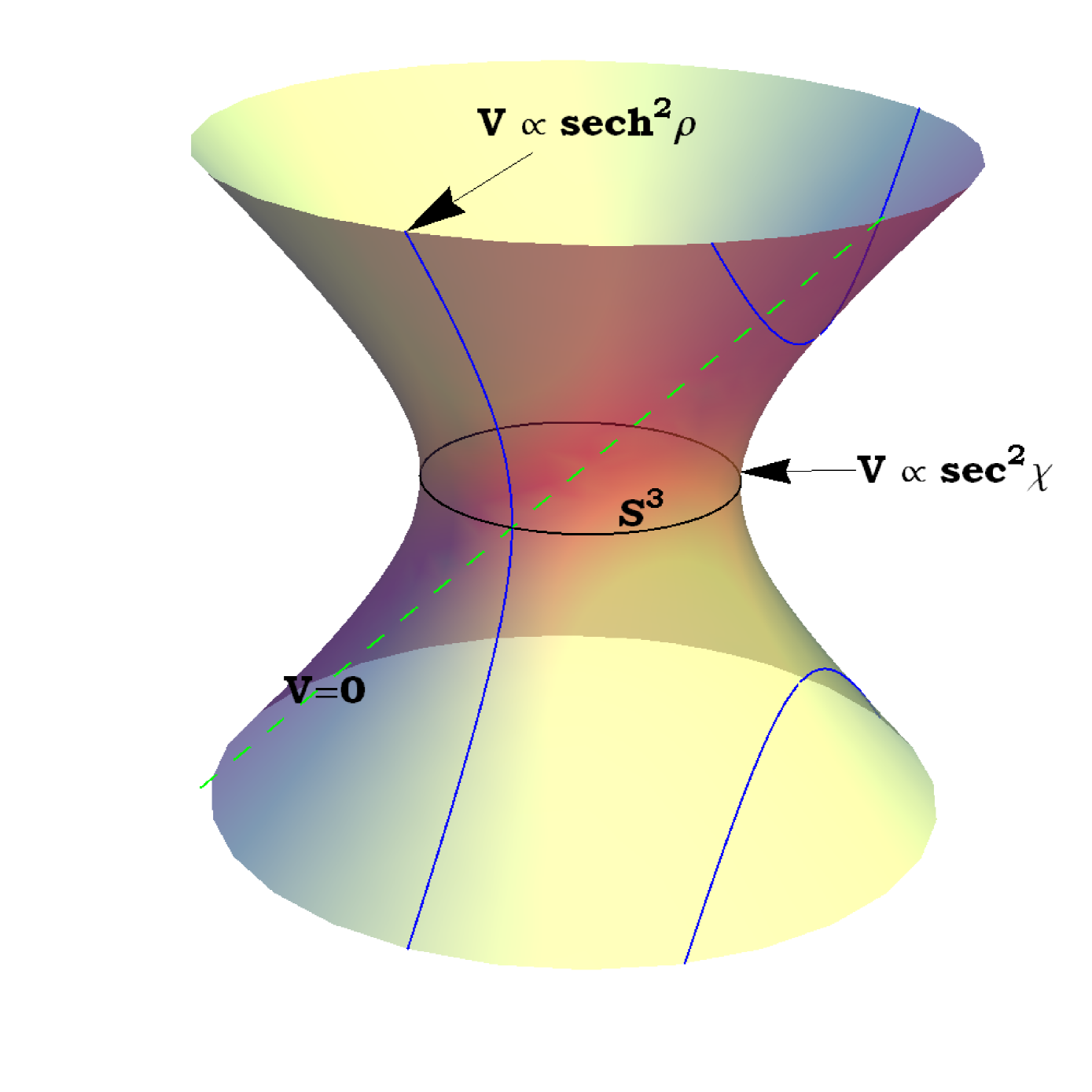
Figure 1: Schematic presentation of the four-dimensional hyperboloid of one shell, the de Sitter space time, $dS_{4}$, embedded in a five-dimensional Minkowski space-time, $M^{4,1}$, some of its geodesics, and their associations with one-dimensional potentials. The equator is a three-dimensional hypersphere, $S^{3}$, and a closed space like geodesic. In terms of a Schrödinger equation, quantum motion on this space is associated with the one-dimensional $V_{\mbox{Sc}}(\chi)$ potential in (2). The open hyperbolic geodesics are three-dimensional $dS_{3}$ hyperboloids. The corresponding one-dimensional potential, is $V_{\mbox{PT}}(\rho)$ in (5) for $\lambda=(K+1)$. The straight lines correspond to inertial motions on three planes. The symmetry of the sec${}^{2}\chi$ potential is given by the isometry group $SO(4)$ of $S^{3}$, while that of $\textrm{ sech }^{2}\rho$ is the $dS_{4}$ isometry $SO(4,1)$, the respective maximal compact and maximal non-compact subgroups of the conformal group $SO(4,2)$. The conics obtained through the slicing by planes parallel to the vertical time axis have the structure of three dimensional Lobachevsky space-times, ${\mathbf{H}}_{\pm}^{3}$, and describe causal patches on $dS_{4}$ [29].

3 Complexification of the Pöschl-Teller well to a barrier, scattering matrix and poles

In order to transform the well potential in (5) into a barrier it is sufficient to change its sign [27], which is achieved by the following complexification (analytical continuation) of the $\lambda$ parameter in (9):

$$\lambda \longrightarrow i\lambda=i\left(K+1\right).$$ (29)

In so doing, one arrives at the following barrier,

$$V_{\mbox{PT}}(\rho) \stackrel{{\scriptstyle(K+1)\to i(K+1)}}{{\longrightarrow}} \frac{\left(K+1\right)^{2}+\frac{1}{4}}{\cosh^{2}\rho}+A^{2}={\mathcal{V}}_{\mbox{PT}}(\rho).$$

At the level of the $a$ constant in (20), defining the solutions in (21), the complexification prescription translates as,

$$a=\frac{1}{2}+K+1\longrightarrow\frac{1}{2}+i\left(K+1\right).$$ (31)

This is a key relation in the following as it turns out to be of crucial importance of finding a geometry on which the complex poles of the transfer scattering matrix of the Pöschl-Teller barrier feature the property of carrying same degeneracies as the states in a level bound in the $\sec^{2}\chi$ potential in the equation (41) below. The effect of the complexification in (29) on the energy ${\mathcal{E}}^{2}$ in (22) is that it changes from real to a complex one, from now onwards denoted by $\left({\mathcal{E}}^{res}\right)^{2}$. Below we bring the real and imaginary parts of $\left({\mathcal{E}}^{res}\right)^{2}$ separately,

$${\mathcal{R}}e\,\left({\mathcal{E}}^{(res)}\right)^{2}=\frac{\hbar^{2}c^{2}}{R^{2}}\left[\left(K+1\right)^{2}-\left(n_{r}-\frac{1}{2}\right)^{2}\right]+\frac{\hbar^{2}c^{2}}{R^{2}}A^{2},$$

(32)

$${\mathcal{I}}m\,\left({\mathcal{E}}^{(res)}\right)^{2}=2\frac{\hbar^{2}c^{2}}{R^{2}}\left(K+1\right)\left(n_{r}-\frac{1}{2}\right).$$

(33)

From now onwards the $A^{2}$ constant can be set to zero, $A^{2}=0$. Moreover, for the needs of what follows it is convenient to introduce the following notation in terms of a wave vector, $k$, defining the complex energy as,

$$\left({\mathcal{E}}{}^{(res)}\right)^{2} = \frac{\hbar^{2}c^{2}}{R^{2}}k^{2},$$

$$k = -i\left[i\left(K+1\right)+\frac{1}{2}-n_{r}\right]$$ (34)

$$= \left[\left(K+1\right)+i\left(n_{r}-\frac{1}{2}\right)\right].$$

In order for the energies in (34) to be physically observable, one has to show that $k$ defines a pole of the analytically continued transmission scattering matrix.

3.1 Resonances and complex energies

In order to calculate the scattering matrix of the Pöschl-Teller barrier, one needs to know the asymptotic behavior of the wave functions $U(\rho)$ in (19) for $\rho\to\pm\infty$, as it follows from the asymptotic properties of the hyper geometric function in (21). This behavior is known [30], [27] to be given by the following linear superposition,

$$A_{\pm}(k)e^{ikx}+B_{\pm}(k)e^{-ikx},\quad x=i\sinh\rho,$$ (35)

with $k$ in (34). The scattering matrix connects the asymptotic incoming with the asymptotic outgoing wave functions, and can be expressed in terms of the transfer matrix, ${\mathcal{T}}(k)$, defined as,

$$\left(\begin{array}[]{c}A_{+}(k)\\ B_{+}(k)\end{array}\right)={\mathcal{T}}(k)\left(\begin{array}[]{c}A_{-}(k)\\ B_{-}(k)\end{array}\right),\quad{\mathcal{T}}(k)=\left(\begin{array}[]{cc}{\mathcal{T}}_{11}(k)&{\mathcal{T}}_{12}(k)\\ {\mathcal{T}}_{21}(k)&{\mathcal{T}}_{22}(k)\end{array}\right).$$ (36)

This matrix is expressed in terms of Gamma functions and its explicit general form can be found for example in Ref. [27]. For the barrier parametrization of our interest the resulting transmission coefficient, denoted by $T(k)$, can be cast into the following form, [27]

$$T(k) = \frac{\mbox{sinh}^{2}\pi k}{\mbox{cosh}^{2}\pi k+\mbox{sinh}^{2}\pi(K+1)}.$$ (37)

It is easy to cross-check that the $T(k)$ denominator nullifies for the precise $k$-value given in (34), as expected,

$$\mbox{cosh}^{2}\pi k+\mbox{sinh}^{2}\pi(K+1)=0,$$

$$\mbox{for}\quad k=\left[(K+1)+i\left(n_{r}-\frac{1}{2}\right)\right],$$ (38)

thus in confirmation of the anticipated observability of the complex energies in the equations (32)-(34). Therefore, setting $n_{r}=$const in (32), one finds out how the real part of the squared complex energy $\left({\mathcal{E}}{}^{(res)}\right)^{2}$ looks like at $\rho=0$, i.e. at the $dS_{4}$ equator, $S^{3}$. Subsequently, these poles will be at times referred to as Pöschl-Teller (PT) resonances.

3.2 Comparison between the PT resonances and the states bound within the trigonometric Scarf well

The important aspect of the expression for the real part in (32) of the squared resonance energy in (34) is that it equals, modulo an additive constant, the squared energies, here denoted by $\left({\mathcal{E}}{}^{(bound)}\right)^{2}$, of the bound states within the $V_{\mbox{Sc}}(\chi)$ potential in (2), earlier studied in detail in [17] as part of the complete trigonometric Scarf potential. Without repeating the details of [17], we notice that also this potential can be shown to emerge from the eigenvalue problem of, $\left[-\Delta_{S^{3}}(\chi,\theta,\varphi)\right]$, the Laplace operator describing free quantum motion on the hyper spherical $S^{3}$ closed-space like $dS_{4}$ geodesic, as visible from its definition in (17). The corresponding eigenvalue problem reads,

$$-\hbar^{2}c^{2}\Delta_{S^{3}}(\chi,\theta,\varphi)Y_{K\ell m}(\chi,\theta,\varphi)=\frac{\hbar^{2}c^{2}}{R^{2}}$$

$$\times K(K+2)Y_{K\ell m}(\chi,\theta,\varphi),$$ (39)

where $Y_{K\ell m}(\chi,\theta,\varphi)$ are the four dimensional hyper spherical harmonics defined in (11)-(13). Upon re-expressing these harmonics as,

$$Y_{Klm}(\chi,\theta,\varphi)\cos\chi=U_{\ell n}(\chi)Y_{\ell}^{m}(\theta,\varphi),$$ (40)

and back-substituting in (39), one finds the following one-dimensional stationary wave equation for $U_{\ell n}(\chi)$ solving the $\ell(\ell+1)\sec^{2}\chi$ potential,

$$\frac{\hbar^{2}c^{2}}{R^{2}}\left(-\frac{{\mathrm{d}}^{2}}{{\mathrm{d}}\chi^{2}}+\frac{\ell(\ell+1)}{\cos^{2}\chi}\right)U_{\ell n}(\chi) = \left({\mathcal{E}}^{(bound)}\right)^{2}U_{\ell n}(\chi),$$

$$\left({\mathcal{E}}{}^{(bound)}\right)^{2}=\frac{\hbar^{2}c^{2}}{R^{2}}(K+1)^{2}, \chi\in\left[-\frac{\pi}{2},+\frac{\pi}{2}\right].$$ (41)

To the amount, the energy at rest equals the invariant mass, the equation (41) can be also read as a mass spectrum,

$$\left(M^{(bound)}\right)^{2}\equiv\left({\mathcal{E}}^{(bound)}\right)^{2}=\frac{\hbar^{2}c^{2}}{R^{2}}(K+1)^{2}.$$ (42)

Furthermore, the $n_{r}$ dependent term in (32) can be absorbed by the real part of the (squared) energy of the resonance, leading to the following definition of the real part of the resonance mass square,

$$\left(M^{(res)}\right)^{2}={\mathcal{R}}{e}\,\left({\mathcal{E}}{}^{(res)}\right)^{2}+\frac{\hbar^{2}c^{2}}{R^{2}}\left(n_{r}-\frac{1}{2}\right)^{2}$$

$$=\frac{\hbar^{2}c^{2}}{R^{2}}(K+1)^{2}.$$ (43)

In so doing, the consistency of these masses with the masses of the states of equal quantum numbers when complementary and approximately treated as bound in (42) is achieved as,

$$\left(M^{(res)}\right)^{2}=\left(M^{(bound)}\right)^{2}\equiv M^{2}=\frac{\hbar^{2}c^{2}}{R^{2}}(K+1)^{2},$$ (44)

where $M$ is the invariant mass. Recall, the branching ratios,

$$K=n+\ell,\,\,\ell=0,1,2,...,K,\,\,m=-\ell,...0,...,+\ell,$$ (45)

following from (18), and complementing the equation (28). In consequence, the energies in each one of the two spectra in (42) and (43) are $\sum_{\ell=0}^{\ell=K}(2\ell+1)=(K+1)^{2}$-fold degenerate. Such degeneracy patterns, in combination with be it an infinite number of levels, for the case of the bound spectrum, or the infinite number of poles, for the case of the resonance trajectories, are a typical signature of a conformal symmetry [21].

Figure 2: Schematic presentation on the $\ell^{P}/M$ plane (with $P$ standing for spatial parity) of a linear conformal Pöschl-Teller (PT) resonance trajectory. Here, the mass is given in dimensionless units, $\left[\mbox{GeV}\right]\left[R\right]/\left[\hbar c\right]$, for simplicity, where $\left[R\right]$=fm. The horizontal straight lines mark finite dimensional representations of the four dimensional rotational group $SO(4)$ corresponding to the levels of the trigonometric Scarf well, their principal quantum number, the four-dimensional angular momentum $K$, being given to the very right. The ordinary angular momentum content of the $SO(4)$ levels, defined by the branching rule in eq. (45), and for natural parities $(P)$, can be read off from the horizontal axis. The diagonal lines correspond to constant $n$ values and join resonances defined by the PT barrier according to (48). The spectrum it is totality represents a linear conformal PT resonance trajectory, i.e. the trajectory with $SO(4)$ symmetric poles in (47).

The issue is that because the isometry of the $S^{3}$ hypersphere is $SO(4)$, the maximal compact subgroup of the conformal group $SO(4,2)$, the wave functions of the bound states are these very same ultra spherical harmonics, $Y_{K\ell m}(\chi,\theta,\varphi)$, previously defined in (12). For this reason, the $\sec^{2}\chi$ levels are labeled by the four dimensional angular momentum, $K$ as a principal quantum number, and so are the resonances after the $n_{r}$=const “slicing” in the higher dimension. Moreover, because on the other side $S^{3}$ also represents the curved position space of a Minkowski space time, ${\mathcal{M}}^{3,1}\in dS_{4}$, obtained by conformal compactification of the conformal $(4+2)$ dimensional space time [19], the spectrum as a whole, displayed in in Figure 2, falls into an infinite unitary representation of the conformal group, $SO(4,2)$ [20]. In this way, the spectra in (44) simultaneously implement the conformal symmetry of the $\ell(\ell+1)\sec^{2}\chi$-well potential problem on the one side, and of the real parts of the squared complex energies corresponding to the poles of the transfer matrix of the $[(K+1)^{2}+1/4]\textrm{ sech }^{2}\rho$ barrier, on the other. This scheme provides the scenario for the conformal symmetry based classification scheme of mesons, considered in the next section.

4 Pöschl-Teller (PT) resonance trajectories for high-lying light-flavor mesons and conformal symmetry based systematics

The bound and resonance states spectra in the above equations (42), (43), and (44) are in reality linear in the orbital angular momentum, $\ell$, according to,

$$M^{(bound)}=M^{(res)}\equiv M=\frac{\hbar c}{R}(K+1)=\frac{\hbar c}{R}(n+\ell+1),$$ (46)

where $M$ is the invariant mass. These equations can be viewed in a twofold way, as a linear dependence of the four-dimensional angular momentum on the invariant mass,

$$K(M,R)=\alpha(R)M-1,\quad K=0,1,2,..., \alpha(R)=\frac{R}{\hbar c},$$

$$\quad\left[\alpha(R)\right] = \mbox{MeV}^{-1},$$ (47)

or, as a linear dependence of the total angular momentum, $\ell$, on both the mass and $n$, the number of nodes in the wave function,

$$\ell(M,R)=\alpha(R)M-n-1, \ell=0,1,2,...,\quad\ell+n=K,$$

$$K = 0,1,2,...$$ (48)

For $n$ taking all the allowed values from $0$ to $K$, the $SO(4)$ levels of the Scarf well are recovered, while each $n$=const value defines a linear resonance trajectory corresponding to the Pöschl-Teller barrier. In unfolding the dependence in (47) on the $\ell/M$ plane according to (48), and assuming $CP$ conservation, resonance trajectories of the type given in Figure 2 are obtained. They fall into infinite dimensional unitary representations of the conformal group, a reason for which such trajectories will also be termed to as conformal Pöschl-Teller (PT) resonance trajectories.

As already discussed in the introduction, dependencies of the angular momentum on the invariant mass are generally known as Regge trajectories although the canonical Regge trajectories refer to a linear dependence of the angular momentum on the squared invariant mass of the type [2],

$$\ell(M^{2},t)=\alpha(t)M^{2}+\alpha(0),\quad\left[\alpha(t)\right]=\mbox{MeV}^{-2},$$ (49)

where the argument of the slope, $\alpha(t)$, is the $t$ channel Mandelstam variable. The dependence in (49) appears within string approaches to resonances. We here instead have taken the path of quantum mechanics with the aim to design a correspondence between bound and transmission resonant states. As it will become clear in due course, data on meson excitations support pretty well the resonance trajectories in (47)-(48) which we occasionally will also term to as “quantum mechanical” resonance trajectories. Moreover, our prediction in (47) on the $O(4)\subset SO(4,2)$ symmetry of the aforementioned trajectories is consistent with same symmetry shared by Regge trajectories of $O(4)$ symmetric poles, earlier considered by various authors especially in scattering of particles of equal masses and in the $u$ channel, where the four-dimensional angular momentum is conserved [11], [12], [13]. However, while in the latter works the symmetry has been of purely algebraic nature, we here back it up by the conformal potential dynamics. It is to be noticed that the Laplacian in (17) leads to spatial meson wave functions describing the excitation modes of a rigid rotor, i.e. of the rotational modes of two bodies at fixed time-independent (rigid) distances from their center of mass. At the present stage of development of our model (to be refined below) the nature of the two bodies can not be uniquely specified and can only be conjectured. Some indirect hints are provided through the shape of the potential in the equivalent one-dimensional wave equation in (41). At small angles, the $\sec^{2}\chi$ series expansion gives the Harmonic Oscillator,

$$\frac{\hbar^{2}c^{2}}{R^{2}}\ell(\ell+1)\sec^{2}\chi \approx \frac{\hbar^{2}c^{2}}{R^{2}}\ell(\ell+1)\left[1+\chi^{2}+{\mathcal{O}}\left(\chi^{2n}\right)\right],$$

$$n \geq 2,$$ (50)

a circumstance that makes it more suitable for simulating interactions between more complex meson constituents than the pure quark-anti-quark pairs (typically kept together by a stringy potential) thus in principle admitting for, say, unconventional mesons composed by $(q\bar{q})$- and/or $(q\bar{q})G$ ”molecules” in the spirit of [31]. We shall discuss this point in a due place below.

Linearities as those in (47)-(48) require equidistance between the masses, while the linearity in (49) requires equidistance between the squared masses. While the first condition finds itself confirmed by data to a good accuracy, the second one is notably violated especially on plots in which $M^{2}$ has been given in units of MeV² (see [5], [6]). In the next section we show that the conformal quantum mechanical PT resonance trajectories turn out to be pretty well suited for the description of the high-lying light flavor mesons with masses above $\sim$1400 MeV and below $\sim$2350 MeV.

4.1 Classifying reported light-flavor mesons according to linear PT trajectories

In the present section we analyze data [1] on light-flavor isoscalar–, and isotriplet mesons of both natural and unnatural parities. Besides the full meson listings, use of the “Other light mesons” list has been made. We classify on the $\ell/M$ plane 71 of those mesons with masses below $\sim$2350 MeV according to four conformal resonance trajectories of the type in (48), with ground states corresponding to the $f_{0}$, $\pi$, $a_{0}$, and $\eta$ mesons of lowest masses, displayed on the respective Figures 3, 4, 5, and 6. Each trajectory has been assumed to be characterized by a set of fixed internal quantum numbers corresponding to isospin and $CP$ parity. The overall impression one gets by inspection of the four figures is that with the increase of the mass, the mesons start adjusting better and better to straight lines. The mesons with the lowest masses are commonly organized into the $SU(3)$ (not shown here) flavor octet structures although the $K=1$ $SO(4)$ doublets, $(\ell=0^{\pm},\ell=1^{\mp})$, are already present also in this region for all four meson families. Such doublets are constituted by the $[f_{0}(980)$–$\omega(783)]$, $[a_{0}(980)$–$\rho(770)]$, $[\pi(1300)$–$b_{1}(1235)]$, and $[\eta(1295)$–$h_{1}(1170)]$ pairs, all of which carry the correct quantum numbers required by the conformal trajectories, although their splittings from the respective ground states, and the next excited states do not follow the theoretically predicted equidistance. In the next subsection we shall attend to this issue in greater detail. Namely, there we shall show that a data fit with a conformal extension of the $\sec^{2}\chi$ potential can account for this effect. On total, we accommodate 71 observed and predict 12 “missing” mesons. However, it needs to be said that the particle’s widths do not follow the pattern in (33) prescribed by the external conformal symmetry and a deeper insight needs to be gained into the internal hadron dynamics to understand their behavior in greater detail.

One more intriguing observation we have to report concerns the relevance of the (admittedly approximate) chiral symmetry of the QCD Lagrangian within the light flavor sector of the $u$ and $d$ quarks from the first generation, i.e. of its symmetry with respect to continuous transformations of the type $\left[\exp\left(i\frac{\vec{\alpha}\vec{\tau}}{2}\otimes{\mathbf{1}}_{4}\right)\exp\left(i\frac{\vec{\beta}\vec{\tau}}{2}\otimes\gamma_{5}\right)\right]\left[\chi\otimes\psi\right]$ where the components of $\vec{\tau}$ are the Pauli matrices in isospin space, $\vec{\alpha}$, and $\vec{\beta}$ are parameter triplets, $\psi$ is a Dirac field, while $\chi$ stands for the fundamental doublet of the $SU_{I}(2)$ group of isospin. The symmetry can be described by means of the well known linear $\sigma$ model. This (Lagrangian) model is $SO(4)$ symmetric, though in isospin space, and based on a four-dimensional massless $(1/2,1/2)$ iso-multiplet that contains next to an isoscalar $f_{0}$ meson, also an isovector $\pi$ meson. The latter quadruplet is placed within a double well potential allowing for a non-vanishing (anomalous) vacuum expectation value of the isoscalar field, in consequence of which it becomes possible for the scalar meson to acquire a finite mass, while the isovector meson remains massless. Within this “spontaneously broken” mode of chiral symmetry realization, a massive isoscalar $f_{0}$ and a massless isovector $\pi$ mesons are considered as “hidden” $0^{\pm}$ chiral partners. If the theory were to be free from anomalous expectation values, chiral symmetry had to be realized instead in the manifest Wigner-Weyl mode which would require the $f_{0}$ and $\pi$ mesons to be of equal masses. In general, chiral symmetry requires the duplication in parity of particles of equal spins, and allows their isospins to be distinct by up to one unit. With this in mind, it is now instructive to compare the $f_{0}$ and $\pi$ trajectories and to check as to what extent the mesons placed on them can be viewed as chiral partners. Such a partnership in the sense of a “hidden” chiral symmetry suggests complete duplication of the particles participating the $SO(4)$ poles of natural parities on the isoscalar $f_{0}$ trajectory by particles participating the $SO(4)$ poles of unnatural parities on the isovector $\pi$ trajectory, however without demanding coincidence of their masses, something which is fully satisfied for the lower lying $K=1$ and $K=3$ poles. However, for the highest $K=4$ and $K=5$ poles, where only the $b_{5}$ partner to the $\omega_{5}(2250)$ state is missing, the natural parity $SO(4)$ poles from the $f_{0}$ trajectory present themselves almost mass-degenerate with the unnatural parity $SO(4)$ poles from the pion trajectory, and more in accord with the Wigner-Weyl mode of chiral symmetry realization. Similarly, also the $a_{0}$ and $\eta$ trajectories could be viewed as chiral partners, and the above discussion would equally well apply to them too. In this way the classification scheme under discussion relates to chiral QCD dynamics. However, the chiral symmetry of the canonical QCD Lagrangian in the $(1+3)$ dimensional Minkowski space time does not require and can not explain the observed degeneracy correlations among the masses of parity couples characterized by different spins. This latter phenomenon requires for its explanation the involvement of a symmetry bigger than the traditional chiral one, which we here identify as the conformal symmetry. On the other side, chiral symmetry in conformal space-time would refer to parity duplicated irreducible unitary $so(2,4)$ representation spaces, to which the conformal families of trajectories displayed in the Figures 3-7 have been set in correspondence. In this way, the spectra in the Figures 3-7 could be indicative of chiral dynamics in conformal space time. Within this context, the masses of the mesons in the two poles of the highest $K$ values observed, located in the region between $\sim$2000 MeV to $\sim$2350 MeV, could indicate the scale at which the restoration of the chiral symmetry from the Goldstone to the Wigner-Weyl mode is likely to take place.

Figure 3: Classification of the isoscalar natural parity $f_{0}$-meson type excitations according to a conformal resonance trajectory of the kind displayed in Fig. 2. Isospin and $CP$ parity are same for all mesons on the trajectory. The masses are given in units of MeV for the sake of having better match with the notations of the mesons, where the number in the parenthesis is representative for the world average of the measured mass in MeV. The data are taken from [1]. All $\omega$ mesons from the $K=4$ and $K=5$ poles have been taken from the list of “Other light mesons”. Other notations as in Fig. 2. The leading trajectory reveals the most significant deviation from the straight line but this falls into the low-energy and low-$K$ values region, where unitary and conformal symmetries interfere. However, above $\sim$1300 MeV, and for $K\geq 2$ the trajectories notably straighten. This is the scale from which onward in our opinion the conformal symmetry starts holding valid to a good accuracy. The $\omega$ meson trajectories, usually displayed separately [3], are within this scheme a subset of the $f_{0}$ trajectories. The $f_{0}$ and $\pi$ trajectories can be viewed as chiral partners (see discussion in Fig. 4).

Figure 4: Classification of the isotriplet unnatural parity $\pi$-meson type excitations according to a conformal resonance trajectory of the kind displayed in Fig. 2. Data taken from [1]. Other notations same as in Figure 3. Two pions and three $b$ meson states, denoted by $\pi(...)$ and $b_{\ell}(...)$ with $\ell=1,3,5$, respectively, are missing for the completeness of the $SO(4)$ poles on the figure. Above $\sim$1800 MeV the trajectories start notably straightening. To the amount within the $\sigma$ model the $f_{0}(500)$ could be considered as the chiral partner to $\pi(139)$, the $f_{0}$ and $\pi$ trajectories could be viewed as chiral partners too. Notice that above $\sim$ 2000 MeV, the masses of the natural and unnatural parity $SO(4)$ poles with $K=4$ and $K=5$ from the respective $f_{0}$ and $\pi$ trajectories, become very close. Admittedly, with the exception of $\pi_{2}(2100)$, all the other resonances from the $K=4$ and $K=5$ poles have been taken from the list of “Other light mesons”. At lower masses, the pole splittings remain still significant. The scale of chiral symmetry restoration for the light flavor mesons in the stronger sense (see discussion in the text) is expected to happen above $\sim$2000 MeV.

Figure 5: Classification of the isotriplet natural parity $a_{0}$ meson type excitations according to a conformal resonance trajectory of the kind displayed in Fig. 2. Data taken from [1]. There are three $a_{0}$ states, denoted by $a_{0}(...)$, missing for the completeness of the spectrum. Other notations as in Figure 3. The higher lying trajectories are straight lines to a reasonable accuracy. In parallel to the $f_{0}$ case, we here consider the trajectories of the $\rho$ meson (the triplet partner to the isoscalar $\omega$ meson) as a subset of the $a_{0}$ trajectories and not as usually displayed [3], as independent trajectories. The figure shows that above $\sim$1400 MeV the trajectories on the $\ell/M$ plane are to a good accuracy straight parallel lines. Similarly to the $f_{0}$ and $\pi$ trajectories, also the $a_{0}$ and $\eta$ trajectories are likely to be chiral partners. Exactly in same regions as for the $f_{0}$ and $\pi$ trajectories, namely around $\sim$2000 MeV and $\sim$2300 MeV, the masses of the natural and unnatural parity $SO(4)$ poles with $K=4$ and $K=5$ get very close. However, all the $a_{\ell}$ mesons in this region have been taken from the list of “Other light mesons”. At lower masses, the pole splittings remain still significant. Also for the chiral pair of the $a_{0}$ and $\eta$ resonance trajectories, the chiral symmetry restoration in the stronger sense (discussed in the text) is likely to happen above $\sim$2000 MeV.

Figure 6: Classification of the isoscalar unnatural parity $\eta$ meson type excitations according to a conformal resonance trajectory of the kind displayed in Fig. 2. Data taken from [1]. The first $\eta_{2}$, $\eta_{4}$, and $h_{3}$ and $h_{5}$ states are “missing” for the completeness of the spectrum. Other notations as in Figure 3. The higher lying trajectories are straight lines to a reasonable accuracy. The figure shows that above $\sim$ 1500 MeV the trajectories on the $\ell/M$ plane are in addition to a good accuracy parallel lines. In the $K=4$ and $K=5$ levels, with the exception of the $\eta(2225)$ and $\eta_{2}(1870)$ mesons, all the other resonances have been taken from the list of “Other light mesons”. This trajectory can be viewed as the chiral partner to the $a_{0}$ one (see discussion in Figure  5).

The conformal symmetry of mesons has previously been noticed and discussed also in [4], [9], and [32]. Our analysis, modulo few different assignments, basically because of data upgrades, is pretty close to that performed by Afonin in [4], [33]. However, the physical background of our classification, and the conclusions drawn from our analysis, go beyond those in [4], where the conventional Regge trajectories in (49) on the $\ell/M^{2}$ plane have been employed. We here have instead first identified a quantum mechanical barrier potential as the culprit behind the conformal patterns of the resonances, whose energies are defined by the poles of the associated transmission scattering matrix. Then we could correlate those patterns with states bound within a conformally symmetric well potential.

Finally, a comment is in place on the mesons from [1] which so far have not been included here. In first place these are the $f$, $a$, and $\eta$, and $\pi$ mesons of odd spins, and the $\omega$, $\rho$, $h$, and $b$ mesons of even spins. These groups of mesons appear on the $f_{1}$, $a_{1}$, $\eta_{1}$, and $\pi_{1}$ trajectories. These trajectories are of a quality more or less comparable to the ones analyzed here and have been omitted for the only sake of not overloading the presentation. More seriously, in the energy range under investigation we found the following 11 mesons which dropped out of our suggested systematics: (i) the one $\rho$ meson, $\rho(1570)$, (ii) the ten $f$ mesons, $f_{0}(1500)$, $f_{0}(2100)$, $f_{0}(2200)$, $f_{2}(1270)$, $f_{2}(1565)$, $f_{2}(1810)$, $f_{2}(1910)$, $f_{2}(1950)$, $f_{2}(2150)$, $f_{2}(2340)$. In order to gain some insight into the abundant presence of $f$ mesons in [1] we notice that mesons like $f_{0}(500)$, $f_{0}(980)$, $f_{0}(1370)$, and $f_{0}(1710)$ debated in the literature to have same internal structure (be it quark-antiquark, $(q\bar{q})$ [34], or of a singlet-glueball $(q\bar{q})_{0}G$ [35]) appear placed also within our classification scheme on the same trajectory. In view of this observation, the abundant $f_{0}$ mesons could be of a structure different from that of the particles populating the trajectory. Which precisely, remains an open question which can not be answered within the model under discussion. Ours is an algebraic potential model, whose prime purpose is to draw attention and provide a scenario suitable for the description of the striking multiple degeneracies observed in the meson spectra in terms of a symmetry possibly relevant for the theory, and which does not allow one to distinguish between the above two pictures of microscopic structure. However, within the context of the discussion after the equation (50) above, one should not exclude the option that the $f_{0}$ particles on Figure 3 might throughout be close to a particular type of unconventional mesons. One more point that deserves attention concerns the dependence of the suggested classification scheme on the so far uncertain status of the resonances taken from the list of “Other light mesons” in [1]. First of all we like to emphasize that the scheme employed so far does not take into account important aspects of the internal dynamics. Specifically, threshold effects could frustrate the formation of some of the states predicted by the conformal symmetry, while many-body effects can cause co-existence of distinct symmetry patterns in the spectra, a phenomenon well documented in nuclear physics where one can observe coexistence of isolated single-particle and correlated collective rotational excitations in the spectra of collective nuclei. Without entering into the technical details of this phenomenon, which can be extended to apply to the case of our interest too, we here limit ourselves to notice that the notion of “partial symmetries” has been coined in [36], where examples of Hamiltonians adequately describing these properties have been constructed. Our case here is that a clear footprint of the conformal symmetry is seen in the meson spectra. At which scale, through which effects, and to what extent this symmetry could be broken, is a challenging and important issue worth of being investigated in more detailed models of internal meson structure than the one considered here. As to the allegedly breaking of the conformal symmetry by the dilaton mass, we like to remark that an external scale can but must not necessarily break an algebraic symmetry, and one has to attend to this question separately by modelling both alternatives and comparing to data. After the equation (52) we specifically discuss how the conformal symmetry can be realized in the presence of two external scales, and if the one of them were to be in some way related to the dilaton mass, the latter still could leave the symmetry intact.

In conclusion, the satisfactory data classification of the high lying mesons by means of the conformal symmetry respecting duality between hadronic bound states and transmitted resonances hints on the relevance of conformal symmetry for strong interaction processes.

4.2 Data fit by the (sec${}^{2}\chi$ +tan$\chi$) potential

As already observed above, and visualized by the Figures 3-6, the linear $\ell(M,R)$ dependence in (48) between the spins and the masses of the mesons begins applying from about $\sim 1400$ MeV onwards. Below, the deviations of the masses of the $SO(4)$ poles from the equidistance required by (48) are severe and hint on the insufficiency of the $\sec^{2}\chi$ potential to correctly capture the dynamics at low energies. However, a remedy to the problem is provided upon upgrading the $\sec^{2}\chi$ well by a potential shaped after a tangent function, shown in the Appendix A to represent a conformal symmetry respecting dipole interaction within a color-neutral two-body system. This confining color dipole potential is introduced in the equation (60), and its equivalent, calculated from a cusped Wilson loop, is given in the equation (101) in the Appendix B. The potential in (101) is shaped after a cotangent function and is related to (60) through a shift of $\chi$ towards $\chi\longrightarrow(\chi+\pi/2)$. The net $(\sec^{2}\chi+\tan\chi)$ potential, denoted by $V^{(b)}_{\mbox{tRM}}(\chi)$, and employed in the data fit in the current section, is given in (67), however in dimensionless units. Then the parameters of the $\left(\epsilon^{(b)}_{\ell n}\right)^{2}$ spectrum formula in (67), can be adjusted by least square fit to the masses of the low lying mesons for any one of the four trajectories. For this purpose, we return to the physical units of the energy, $\left[\hbar^{2}c^{2}/R^{2}\right]\left(\epsilon^{(b)}_{\ell n}\right)^{2}$, and set it equal to the squared mass, $M^{2}$, now expressed in units of GeV², arriving at the following mass formula,

$$\frac{\hbar^{2}c^{2}}{R^{2}}\left(\epsilon_{\ell n}^{(b)}\right)^{2}\equiv M^{2}=A(R)(K+1)^{2}-\frac{B(R)}{(K+1)^{2}}+C,$$

(51)

$$A(R)=\frac{\hbar^{2}c^{2}}{R^{2}},\,\,\left[R\right]=\mbox{fm},\quad B(R)=\left(\frac{b\hbar c}{R}\right)^{2},$$

$$\left[A(R)\right]=\mbox{GeV}^{2},\quad\left[B(R)\right]=\mbox{GeV}^{2},\,\,\left[C\right]=\mbox{GeV}^{2},$$

(52)

where $R$ stands for the $S^{3}$ (hyper)radius. Contrary to (48), the $\ell(M)$ dependence following from (51) is no longer linear. Notice that the spectrum in (52) continues respecting the conformal degeneracy patterns of (41) though it contains next to the first external scale given by the hyper-radius $R$, a second one, the magnitude $B(R)$ of the tangent term. If the $B(R)$ parameter were to be in some way related to the dilaton mass, then the latter could throughout leave the conformal symmetry intact. In more technical terms, it can be shown that the Hamiltonian in (65) is intertwined with the $\chi$ dependent part of the Lapalcian in (17). The parameter values fitting the data are listed in the Table 1. The slope parameter, $A(R)$, has been kept fixed for all four trajectories, while the remaining two parameters, $B(R)$ and $C$, were allowed to change from trajectory to trajectory with the aim to fit the gaps between the ground and the first excited states. The $\tan\chi$ term in (67), equivalently, the term proportional to $B(R)$ in (51), contributes significantly anyway only to the gaps between the poles characterized by the lowest $K$ values. For $K\geq 2$ values it becomes practically irrelevant and does not affect the linearity of the trajectory at this scale. The results of the data fits, compiled in Fig. 7 and the Tables 1-3, are in good agreement with the measurements.

In the Table 2 we list our predictions for the masses of the 12 “missing” mesons discussed above.

In Table 3 we present as an illustrative example of the findings of this work a comparison between the measured and the predicted masses of the mesons on the pion trajectory. The data fits to the mesons on the remaining trajectories are of the same quality and are not given here for the sake of not overloading the presentation.

As already mentioned to the end of the opening of this section, our model is exclusively focused on the importance of the external conformal symmetry in shaping the spatial parts of the meson wave functions with the aim to provide an explanation for the observed striking $SO(4)$ degeneracies. The nature of the two meson constituents can only be indirectly deduced from the properties of their interaction. To the amount the upgrading interaction used in our analysis is closely related to the Cornell potential, known to describe not only quark-antiquark but also gluon-gluon ($G-G$) interactions [37], we admit for the possibilities that the internal meson configuration can contain $(\bar{q}-q)$ next to $(G-G)$ pairs. Within a scheme of such limitations, no prediction on the internal quantum numbers of the mesons, i.e. on their isospins, the $G$ and $C$ parities, can be made. As a guidance in the assignment of the mesons to the trajectories and their $SO(4)$ poles, we used only the external quantum numbers corresponding to masses, spins, and spatial parities, which are well defined within the scheme. As additional assumptions, the constancy of the $CP$ parity and isospin over a trajectory has been made. A model capable of predicting the internal quantum numbers of the mesons has to be based upon a microscopic Hamiltonian expressed in terms of quark- and anti-quark creation and annihilation operators, of well defined properties under charge conjugation and reflection within the isospin space. Such a model has been developed in Ref. [38] for the particular case of isocalar mesons on the grounds of a second quantized Hamiltonian and with a schematic interaction, meaning that the interaction strength has been maintained as a free parameter depending on the quantum numbers characterizing the orbitals and the spins of the quark and anti-quark creation and annihilation operators. This model has a total of nine parameters, same as our model.

In order to cross check consistency of our conjectures on the internal meson quantum numbers with the corresponding definitions in [38], we pick up as a trial set five mesons whose quantum numbers are equal in both schemes, and compare the predictions on their masses by the two respective approaches (see Table 4). In finding congruency between these predictions, we conclude on the adequacy of our assumed $I$ , $G$, and $C$ assignments.

Finally, it needs to be noticed that the potential in (67) has been earlier employed by us in the description of baryons, considered as quark-diquark systems, and also there it was shown to provide a very satisfactory data description [9], [40] not only on the spectra but also of the proton electric charge form factor, though in this reference the very essential points on the color dipole character of this potential and on its link to Wilson loops have not yet been understood. We conclude on the relevance of conformally symmetric trigonometric and hyperbolic potentials in quark model physics.

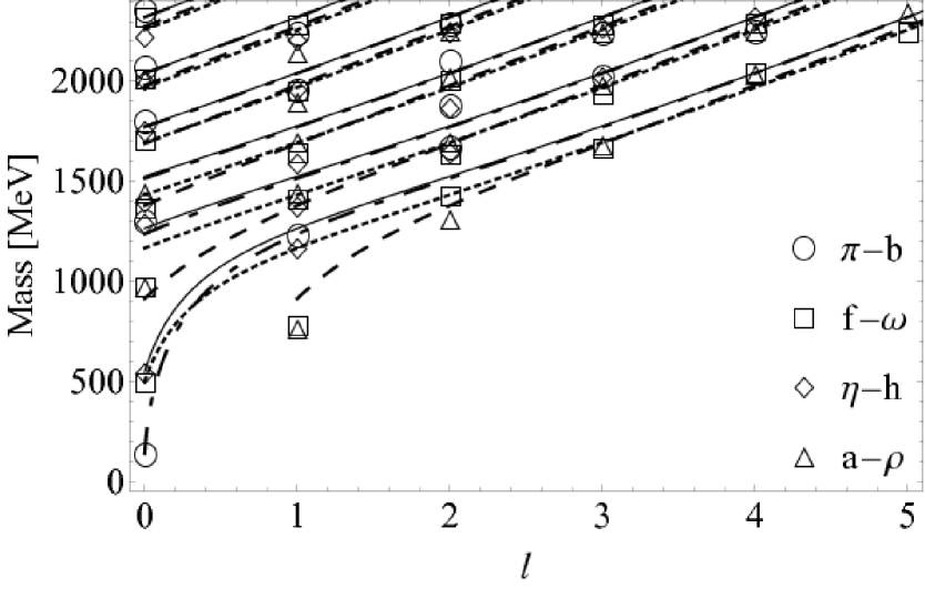
Figure 7: Nine parameter fit by the mass formula in (51) to the twenty four conformal trajectories, corresponding to $\pi(139)$, $f_{0}(500)$, $\eta(550)$, and $a_{0}$ resonances. The “missing” $a_{0}(...)$ ground state has not been taken into account. The six dashed-dotted lines represent our fit to the six pion sub trajectories on the $\ell/M$ plane, while the circles indicate the mass positions of the observed resonances, as a comparison. The six solid–, the six dotted-, and the six dashed lines, represent in their turn the fits to the $f_{0}$, $\eta$ and $a_{0}$ trajectories, respectively. The corresponding experimentally observed mesons located on the latter trajectories are denoted by squares, diamonds, and triangles, respectively. The slope parameter $A(R)$ has been kept fixed. The linearity of, and the parallelism among the trajectories above $\sim 1400$ MeV are well pronounced. The parity doubling on the ($f_{0}$-$\pi$) and ($\eta$-$a_{0}$) trajectories is also well pronounced.

5 Summary and conclusions

We developed a unified scheme for the description of mesons as bound states within a well potential, on the one side, and as resonances transmitted through a barrier, on the other. We employed the pair of potentials constituted by the trigonometric Scarf well, $\ell(\ell+1)\sec^{2}\chi$, and the Pöschl-Teller barrier, $\left[(K+1)^{2}+1/4\right]\textrm{ sech }^{2}\rho$, where $\ell$ and $K$ stand in turn for the ordinary and the four-dimensional angular momentum values. This particular choice of the potential parameters guarantees that (i) the real parts of the squared complex resonance energies equal the squared energies of the bound states, (ii) the energies are $(K+1)^{2}$-fold degenerate, thus revealing the conformal symmetry of the spectra. On these grounds we suggested a conformal symmetry based classification scheme of mesons according to linear resonance trajectories with $SO(4)$ poles (conformal trajectories), which we depicted on the plane of the total angular momenta ($\ell$) (the mesons integer spins) versus the invariant masses $(M)$ with $\ell$ obeying the $SO(4)$ pole branching rule of, $\ell=0,1,2,...,K$, and for $K=0,1,..,5$. As examples illustrative of our findings we applied the scheme to the classification of four families of trajectories corresponding to $f_{0}$, $a_{0}$, $\pi$, and $\eta$ meson resonances, on which we could organize into a total of 23 $SO(4)$ poles 71 reported mesons and predict 12 “missing”. Only 11 mesons, from them 10 $f$ mesons, dropped out of the systematics.

We observed that with the increase of the energy and especially above $\sim$1400 MeV, the experimental data start aligning better and better to the predicted linearity of the trajectories thus revealing the adequacy of the trigonometric Scarf well in this mass region. As to the mesons of the lowest masses, the $\sec^{2}\chi$ interaction failed to predict the correct gaps between the ground state and the first excited states. However, this failure has not been attributed to the violation of the conformal symmetry. The fact is that the extension of the trigonometric Scarf well by the conformally invariant color dipole potential in (60), equivalently, the Wilson loop potential in (101), was able to satisfactory describe the aforementioned gaps while continuing respecting the conformal symmetry. In effect, a quite satisfactory nine parameter fit to the 71 classified mesons, distributed over a total of 23 $SO(4)$ poles, could be performed. In addition, our analysis showed that above $\sim$1700 MeV the masses of the $SO(4)$ poles from the respective chiral-partner ($\pi$ - $f_{0}$), and $(\eta$-$a_{0}$) trajectories start notably approaching each other becoming practically mass degenerate, around $\sim 2000$ MeV and $\sim 2300$ MeV, respectively. We interpreted existence of these trajectories in general and the mass degenerate parity duplication of the $K=4$ and $K=5$ $SO(4)$ poles in particular, as a possible signature for chiral symmetry restoration at this mass scale. Though an element of uncertainty is invoked by the status of the resonances placed on the latter poles, predominantly taken from the list of “Other light mesons ” in [1], we nonetheless read this phenomenon as an indication that chiral symmetry for mesons might be realized in terms of parity doubled conformal multiplets rather than, as usually assumed, in terms of parity doubling of single $SO(3)$ states [39].

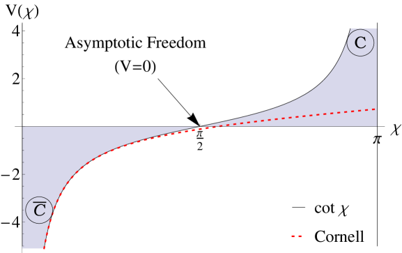
Figure 8: The color dipole potential in the equations (72)-(74) and its characteristics. Charge and anti-charge have been denoted by $C$ and ${\overline{C}}$, respectively.

The unified description of bound states and resonances has been achieved by virtue of the four-dimensional de Sitter space time, $dS_{4}$, on which the well potential shapes the free quantum motion on the closed hyper spherical $S^{3}$ geodesic, while the barrier does same on open hyperbolic geodesics. Further non-trivial insights into the properties of both potentials have been gained in formulating effective chromo-statics on $dS_{4}$. Namely, it has been found in the Appendix A that the nature of such a statics depends on the type of the $dS_{4}$ geodesics. Consistent chromo-statics on the unique closed space like geodesic of $dS_{4}$, the equatorial hypersphere $S^{3}$, imposes severe restrictions on the allowed number of color charges on this space by requiring it to be exactly balanced out by an equal number of anti-color charges. In addition, each single color-charge potential has to be a fundamental solution of the conformal $S^{3}$ Laplacian. Then the color–anti-color system creates a color dipole confining potential, shaped after a tangent ($\tan\chi$), or, a cotangent ($\cot\chi$) function in depending on the range of the argument, $\chi\in[-\pi/2,+\pi/2]$, versus $\chi\in[0,\pi]$, with $\chi$ standing for the second polar angle parametrizing the hypersphere $S^{3}$. The trigonometric $\sec^{2}\chi$ function now takes the part of a color-electric field to this potential. In effect, the $dS_{4}$ space time provides an intriguing geometric set up, suggestive of defining a “geometric confinement” as conformal symmetry motivated color neutrality of quark systems placed on $S^{3}$ closed spaces. This definition, in predicting conformal color–anti-color (two-sources) potentials of the type, $\sec^{2}\chi+\tan\chi$, equivalently, $\csc^{2}\chi+\cot\chi$, could be tested and convincingly confirmed through a fit to a representative part of the light flavor meson spectrum. It needs to be said that the latter interaction, very well known from the supersymmetric quantum mechanics [24] under the name of the trigonometric Rosen-Morse potential, has earlier been used by us also to study baryon spectroscopy in [9],[40]. One of the achievements of the present work relative to the previous ones is to have uncovered its color-dipole nature, visualized in Fig. 8, and its origin from cusped Wilson loops in the equation (101) from Appendix B.

In contrast, on open hyperbolic space times, such as the $dS_{4}$ causal patches, which are Lobachevsky space time conics of one less dimension, ${\mathbf{H}}_{\pm}^{3}$, the number of color charges can be arbitrary, and it is within space times of this kind, where free color could in principle be released and become observable. In this way, the de Sitter space time $dS_{4}$ allows for a geometric expression of confinement. Notice that on ${\mathbf{H}}_{\pm}^{3}$, which does not have any closed space-like geodesics, color neutrality would be possible only on $S^{2}$ spherical conics, the quantum motion on which has to be forced by the color gauge group. We conclude on the importance for quark models of hadrons of the color-dipole trigonometric–, and the free single color hyperbolic potentials, considered in the Appendix B. Finally, again by virtue of the $dS_{4}$ geometry, all the involved potentials could be motivated by fundamental principles in relating them to Wilson loops with cusps, and to radial quantization. All in all we conclude on the usefulness of the $dS_{4}$ space time as a tool for modelling the physics of hadrons in support of ref. [22], and on the relevance of trigonometric and hyperbolic potentials for constituent quark models. To the amount, the $dS_{4}$ space, in representing slices of the conformal $AdS_{5}$ space time, relates to the canonical conformal space time by a conformal map, physics in both sets of coordinates are equivalent, and the limitations on the color quantum numbers of hadrons imposed by the hyper-spherical geometry of the closed space-like $dS_{4}$ geodesic (by itself related to the Minkowski space time by a conformal map) remain valid also in flat space. Within this context, the $dS_{4}$ special relativity could be viewed as an aspect of conformal symmetry. In order to include fermionic hadrons, the color group has to be such that at least two color charges transform as an anti-color, a condition met by $SU(3)_{c}$. This consideration provides a “geometric” argument in favor of the relevance of $SU(3)_{C}/Z_{3}$ dynamics of QCD. As long as the only scales which break beyond doubt the conformal symmetry are the masses of the QCD quarks, the conformal symmetry is expected to loose power within the heavy flavor sector, an observation supported by the relevance of the conformal symmetry breaking Cornell potential in this sector. Instead, for the light flavors, we showed that the power Cornell potential needs an upgrade toward the trigonometric conformally symmetric color dipole potential in (72). For a conformally not symmetric strong dynamics the limitations on color neutrality will no longer be compelling and, in case the conformal symmetry were to be the only reason behind the color neutrality, one may entertain the possibility of observing heavy flavor free color charges. At any rate, in our opinion, conformal symmetry breaking, signaled by possibly significant deviations of the heavy flavor meson spectra from those of the light flavor mesons, could turn out to be a precondition for deconfinement.

Without entering into details, the $dS_{4}$ geometry, also reflects, at the quantum mechanical level, the fundamental relevance of $AdS_{5}/CFT_{4}$ for QCD at high excitations.

Acknowledgments
We express our gratitude to Dr. Abdulaziz Alhaidari for a detailed illuminating correspondence on the properties of the Manning-Rosen barrier.

Appendix A: Chromo-statics on $S^{3}\in dS_{4}$. The sec${}^{2}\chi$ function as an ${\mathbf{E}}$ field of a conformally symmetric color dipole confining potential shaped after a tangent function

The $dS_{4}$ space-time has a rich geometric structure, as visible from the Figure 1. The four dimensional hyperboloid of one shell, embedded in a five dimensional Minkowski space time, can be time-sliced on closed, open or flat subspaces. The closed slices are ${\mathcal{R}}^{1}\otimes S^{3}$ conformal compact space times, the open ones are three dimensional two-sheeted hyperbolic subspaces, here denoted by ${\mathcal{R}}^{1}\otimes{\mathbf{H}}_{\pm}^{3}$, and the flat slices are just $M^{2,1}$ planes. We here are especially interested in the $dS_{4}$ equator, which is the three sphere, $S^{3}$, at $\rho=0$. The hyperbolic angle encodes the size of the $S^{3}$ radius away from the equator, and therefore, as it will be shown in the next section, a time variable, meaning that we here are addressing the static case.

To be specific, we are interested in the possibility to formulate effective (one-color) chromo-statics on $S^{3}$. In parallel to electrostatics, one may start approaching this goal by considering the fundamental solutions to the $S^{3}$ Laplace operator in (17). It is not difficult to cross check that the $(-\frac{q}{4\pi}\tan\chi)$ function, where $q$ stands for a color charge, is such a solution,

$$\Delta_{S^{3}}(\chi,\theta,\varphi)\tan\chi=0.$$ (53)

The tangent function parallels on $S^{3}$ the $(-1/r)$ fundamental solution to the three dimensional flat space Laplacian, $\nabla^{2}$, and could be thought of as a version of a “curved Coulomb” potential [41]. The corresponding ${\mathbf{E}}(\chi)$ field is then obtained as,

$${\mathbf{E}}(\chi)=-\frac{q}{4\pi}\frac{\partial(-\tan\chi)}{\partial\chi}=\frac{q}{4\pi\cos^{2}\chi}=\frac{q}{4\pi}\sec^{2}\chi.$$ (54)

Therefore, the $\sec^{2}\chi$ function is found to shape on $S^{3}$ a static color-electric field, denoted by ${\mathbf{E}}(\chi)$. A similar result, though for electric charges, has been reported in [42], where it has been derived from the Gauß  theorem on $S^{3}$. However, along this line of reasoning one encounters a serious problem. Suppose, for concreteness, that the charge has been located at $\left[\chi=-\pi/2,\varphi=-\pi/2\right]$, referred to here as the “West” pole. Because the outgoing field lines are confined to remain on the hypersphere, they will follow the great circles, which necessarily intersect for a second time as ingoing lines at $\left[\chi=\pi/2,\varphi=\pi/2\right]$, i.e. at the precise anti-pod, the “East” pole, thus creating there a fictitious source whose charge is opposite to the physical one in (54). This is of course an unacceptable unphysical situation in several aspects, one of them, also noticed in [42], concerns the violation of the superposition principle on $S^{3}$. We here solve this dilemma by noticing that this inconsistency appears in consequence of first setting $\rho$ (equivalently, the time) to a constant, and then considering $S^{3}$, instead of first considering the full conformal ${\mathcal{R}}^{1}\otimes S^{3}$ space time and then setting $\rho$ to a constant. As it will be shown in section 5.1 below, in the latter case one encounters the conformal Laplacian, here denoted by, $-\Delta^{1}_{S^{3}}(\chi,\theta,\varphi)$, and presented (in dimensionless units) below in the equation (99) as,

$$-\Delta_{S^{3}}^{1}(\chi,\theta,\varphi) = {\mathcal{K}}^{2}(\chi,\theta,\varphi)+1.$$ (55)

The fundamental solutions (Green functions) ${\mathcal{G}}_{-\frac{\pi}{2}}(\chi)$, and ${\mathcal{G}}_{\frac{\pi}{2}}(\chi)$ to the conformal Laplacian on the hypersphere, corresponding to color-charges placed at $\chi=-\pi/2$, and $\chi=+\pi/2$ (“West” and “East” poles, respectively) are now distinct. They have been calculated for $R=1$ for example in [43], [44] as

$${\mathcal{G}}_{-\frac{\pi}{2}}(\chi) = \frac{1}{4\pi^{2}}\left(\frac{3\pi}{2}-\chi\right)\tan\chi+c_{0},$$ (56)

$${\mathcal{G}}_{+\frac{\pi}{2}}(\chi) = \frac{1}{4\pi^{2}}\left(\frac{\pi}{2}-\chi\right)\tan\chi+c_{1},$$ (57)

where $c_{0}$ and $c_{1}$ are constants. The single color potentials associated with these Green functions are,

$${\mathcal{V}}_{-\frac{\pi}{2}}(\chi) = q_{1}{\mathcal{G}}_{-\frac{\pi}{2}}(\chi)=\frac{q_{1}}{4\pi^{2}}\left(\frac{3\pi}{2}-\chi\right)\tan\chi+q_{1}c_{0},$$

$$q_{1} = -q,$$ (58)

$${\mathcal{V}}_{+\frac{\pi}{2}}(\chi) = q_{2}{\mathcal{G}}_{+\frac{\pi}{2}}(\chi)=\frac{q_{2}}{4\pi^{2}}\left(\frac{\pi}{2}-\chi\right)\tan\chi+q_{2}c_{1},$$

$$q_{2} = q,$$ (59)

respectively. The tangent function in (54) can be recovered but now as a dipole potential produced by two real physical pod-anti-pod charges and expresses in terms of the fundamental solution of the conformal Laplacian in (56)-(57) as,

$${\mathcal{V}}_{-\frac{\pi}{2}}(\chi)+{\mathcal{V}}_{+\frac{\pi}{2}}(\chi)=q_{1}{\mathcal{G}}_{-\frac{\pi}{2}}(\chi)+q_{2}{\mathcal{G}}_{+\frac{\pi}{2}}(\chi) = -\frac{q}{4\pi}\tan\chi,$$

$$c_{1} = c_{0}.$$ (60)

In effect, the ${\mathcal{V}}_{-\frac{\pi}{2}}(\chi)$ and ${\mathcal{V}}_{+\frac{\pi}{2}}(\chi)$ functions describe two different potentials, the first generated by a physical single color charge-, and the second–by a physical anti-color charge, while the tangent function appears as the associated color dipole potential. In this way, the inevitable $S^{3}$ charge neutrality is respected but it stops being unphysical. Now the fields of the physical “negative” ($q_{1}=-q$), and “positive” ($q_{2}=q$) color charges related to the potentials in the equations (58) and (59) are easily calculated and read,

$${\mathbf{E}}_{-\frac{\pi}{2}}(\chi) = -\frac{\partial}{\partial\chi}\frac{q_{1}}{4\pi^{2}}\left(\frac{3\pi}{2}-\chi\right)\tan\chi=\frac{q}{4\pi^{2}}\left(\frac{3\pi}{2}-\chi\right)$$

$$\times \frac{1}{\cos^{2}\chi}-\frac{q}{4\pi^{2}}\tan\chi,$$

$${\mathbf{E}}_{+\frac{\pi}{2}}(\chi) = -\frac{\partial}{\partial\chi}\frac{q_{2}}{4\pi^{2}}\left(\frac{\pi}{2}-\chi\right)\tan\chi=-\frac{q}{4\pi^{2}}\left(\frac{\pi}{2}-\chi\right)$$ (61)

$$\times \frac{1}{\cos^{2}\chi}+\frac{q}{4\pi^{2}}\tan\chi.$$

Their superposition is now well defined and amounts to,

$${\mathbf{E}}_{+\frac{\pi}{2}}(\chi)+{\mathbf{E}}_{-\frac{\pi}{2}}(\chi)=\frac{q}{4\pi\cos^{2}\chi}={\mathbf{E}}(\chi),$$ (62)

which formally coincides with the chromo-static field in (54). However, now the $\sec^{2}\chi$ function has been found as the shape of an ${\mathbf{E}}$ field due to a charge dipole-, and not to a single charge potential, as supposed in (54) and [42]. Therefore, the color-electric field on $S^{3}$ takes the shape of the $\sec^{2}\chi$ function, while the dipole potential is generated by a colorless two-body system, like mesons, and in agreement with the inevitable $S^{3}$ charge neutrality.

Stated differently, on $S^{3}$, which we introduced as the closed space-like geodesic on $dS_{4}$, there can be only color-anti-color charge pairs generating conformal color dipole-potentials, shaped after a tangent function, and an associated conformal ${\mathbf{E}}$ field, shaped after the $\sec^{2}\chi$ function. In this manner, this manifold

• provides a geometric set up suited for modelling confinement within the environmental space as color neutrality of strong interacting systems,

• links this confinement to conformal symmetry of closed space times.

In contrast, on the $dS_{4}$ open hyperbolic geodesics (they are $dS_{3}$ spaces), and/or on the open conic sections, any arbitrary number of color-neutral and single-color systems are allowed to propagate independently from each other. Single color (single source) potentials on $dS_{3}$ are associated with the Green function of the $dS_{3}$ conformal Laplacian (in dimensionless units),

$$-\Delta_{dS_{3}}^{1}(\rho,\theta,\varphi) = -\Delta_{dS_{3}}(\rho,\theta,\varphi)+1,$$ (63)

in which case one encounters in the hyperbolic variable the free color-charge potential as $\left(-\frac{q}{4\pi^{2}}\rho\tanh\rho\right)$. Stated differently, open space times do not require the number of color charges to equal the number of anti-color charges.

As a final remark, we wish to recall that the phenomena considered so far, are all described by space-like physics. Indeed, the well-potential represents an instantaneous interaction, and the barrier potential describes, via tunneling, virtual resonance transmission in scattering. The space-like $dS_{4}$ surface provided the appropriate set-up for their description and interrelation. We conclude on the relevance of $dS_{4}$ symmetry and therefore on $dS_{4}$ special relativity for QCD processes in the space-like region, in support of ref. [22]. Off-shell strong-interactions seem to be sensitive to higher dimensions.

All these clues could be gained thanks to appropriate variable changes and coordinate transformations in the quantum mechanical wave equations, and in combination with convenient choices for the magnitudes of the potentials under investigation.

We also like to remark that exploring a comment by Lovelace [10], we first tried to depart from the spectrum of the $\ell(\ell+1)\csc^{2}\chi$ potential and to transform it into the Manning-Rosen barrier, $\left[(K+1)^{2}+1/4\right]\textrm{ csch }^{2}\rho$, in which case we approached instead of $dS_{4}$, the causal four-dimensional hyperboloid of two sheets, ${\mathbf{H}}_{\pm}^{4}$, also referred to as Lobachevsky’s four plane. However, physics with the Manning-Rosen barrier is quite distinct from that of the Pöschl-Teller barrier. The Manning-Rosen barrier, singular at origin, does not allow for transmission [45],[46],[47] and no duality can be constructed between the bound states within the $\csc^{2}\chi$ well (identical to those of the $\sec^{2}\chi$ well) and states residing in Lobachevsky’s hyperbolic space time. On the latter, no confinement can be defined in terms of quantum motion along geodesics, at most, it could be defined as motion on closed space like conics. Free color charges on ${\mathbf{H}}_{\pm}^{4}$ will give rise to $\left(-\frac{q}{4\pi^{2}}\eta\coth\eta\right)$ potentials, where $\eta$ is now the hyperbolic angle on the respective Lobachevsky space-time.

The above considerations reveal the unifying róle played by large geometric set ups with respect to seemingly disconnected processes in flat space. On curved surfaces, the distinct processes can acquire meaning of different aspects of a more general process.

In this fashion, multidimensional hyperbolic set ups could be employed as useful tools in modelling at the quantum mechanical level of complex physical phenomena.

5.1 Conformal extension of the trigonometric Scarf well by the confining color dipole potential

The dipole potential introduced in (60) in terms of the Green function of the conformal Laplacian, $\left({\mathcal{K}}^{2}(\chi,\theta,\varphi)+1\right)$, has interesting properties with respect to ${\mathcal{K}}^{2}(\chi,\theta,\varphi)$. It commutes with the latter, and acts as an isometry,

$${\mathcal{K}}^{2}(\chi,\theta,\varphi)\tan\chi\,f(\chi,\theta,\varphi)=\tan\chi{\mathcal{K}}^{2}(\chi,\theta,\varphi)\,f(\chi,\theta,\varphi),$$ (64)

where $f(\chi,\theta,\varphi)$ is any arbitrary differentiable function. In other words, the color dipole potential is necessarily $SO(4)$ symmetric. One can now use it as a perturbation of the kinetic quantum motion on $S^{3}$ and write down the following wave equation:

$${\mathcal{H}}(\chi)\widetilde{\psi}^{(b)}_{\ell n}(\chi)=\left(\epsilon^{(b)}_{\ell n}\right)^{2}\widetilde{\psi}^{(b)}_{\ell n}(\chi),$$

$${\mathcal{H}}(\chi)=-\frac{1}{\cos^{2}\chi}\frac{\partial}{\partial\chi}\cos^{2}\chi\frac{\partial}{\partial\chi}+\frac{\ell(\ell+1)}{\cos^{2}\chi}-2b\tan\chi+1.$$

(65)

Upon the variable change,

$$\widetilde{\psi}^{(b)}_{\ell n}(\chi)\cos\chi=U_{\ell n}^{(b)}(\chi),$$ (66)

the equation (65) takes the shape of an one-dimensional wave equation with the so called trigonometric Rosen-Morse potential:

$$\left(-\frac{{\mathrm{d}}^{2}}{{\mathrm{d}}\chi^{2}}+V^{(b)}_{\mbox{tRM}}(\chi)\right)U_{\ell n}^{(b)}(\chi)=\left({\epsilon}_{\ell n}^{(b)}\right)^{2}U_{\ell n}^{(b)}(\chi),$$

$$V^{(b)}_{\mbox{tRM}}(\chi)=\frac{\ell(\ell+1)}{\cos^{2}\chi}-2b\tan\chi,$$

$$\left({\epsilon}_{\ell n}^{(b)}\right)^{2}=-\frac{b^{2}}{\left(K+1\right)^{2}}+(K+1)^{2},$$

$$K=\ell+n,\quad\chi\in\left[-\frac{\pi}{2},+\frac{\pi}{2}\right],$$

(67)

where we set $\hbar=1$, $c=1$, and $R=1$, thus writing down the wave equation in the widely used dimensionless units [24]. In this units, and for $b=0$, the energy $\left({\epsilon}_{\ell n}^{(b)}\right)^{2}$ recovers $\left({\mathcal{E}}^{(bound)}_{2}\right)^{2}R^{2}/(\hbar^{2}c^{2})$ in the equation (41). For $b\not=0$ the $(K+1)^{2}$-fold conformal degeneracy is still respected meaning that the extended potential continues describing a conformally invariant confined colorless system. Therefore, the conformal symmetry on the closed space is fully respected by the color dipole interaction.

Thanks to the negative sign of the $b$ term, the $V^{(b)}_{\mbox{tRM}}(\chi)$ potential provides an efficient tool for increasing the splitting between the ground and lowest excited states in the $\sec^{2}\chi$ well and thus for improving description of meson data, an option of which we make use in the subsequent section. On $dS_{4}$ this potential is converted into the hyperbolic Rosen-Morse potential [24],

$$\left(-\frac{{\mathrm{d}}^{2}}{{\mathrm{d}}\rho^{2}}+V^{(b)}_{\mbox{hRM}}(\rho)\right)U_{\ell n}^{(b)}(\rho)=\left({\epsilon}_{\ell n}^{(b)}\right)^{2}U_{\ell n}^{(b)}(\rho),$$

$$\left({\epsilon}_{\ell n}^{(b)}\right)^{2}=-\frac{b^{2}}{\left(K+1\right)^{2}}-(K+1)^{2},$$

$$K=\ell-n,\quad\rho\in\left[-\infty,+\infty\right],$$

$$V^{(b)}_{\mbox{hRM}}(\rho)=-\frac{\ell(\ell+1)}{\cosh^{2}\rho}-2b\tanh\rho.$$ (68)

To the amount, the $\textrm{ sech }^{2}\rho$ and $\tanh\rho$ potentials emerge from the analytical continuation of the $\sec^{2}\chi$ and $\tan\chi$ potential towards complex values of the argument (in combination with $b\to-ib$), we here take the position that also the hyperbolic Rosen-Morse potential describes quantum motion of colorless systems though such propagating off-shell along open hyperbolic geodesics on $dS_{4}$. In contrast, the free color-charge potential is expected to be shaped after, $\left(-\chi\tanh\chi\right)$.

However, the more familiar notations for the trigonometric Rosen-Morse potentials are those in which the second polar angle, $\chi$, on $S^{3}$ varies as $\chi\in\left[0,\pi\right]$. In this parametrization of $S^{3}$ one finds,

$$\left(-\frac{{\mathrm{d}}^{2}}{{\mathrm{d}}\chi^{2}}+\frac{\ell(\ell+1)}{\sin^{2}\chi}-2b\cot\chi\right)R_{\ell n}^{(b)}(\chi) = \left({\epsilon}_{\ell n}^{(b)}\right)^{2}R_{\ell n}^{(b)}(\chi),$$

$$\chi \in \left[0,\pi\right].$$ (69)

In this coordinate choice the Green functions in (56) and (57) change correspondingly to,

$$G_{-\frac{\pi}{2}}(\chi)\to G_{0}(\chi)=\frac{1}{4\pi^{2}}(\pi-\chi)\cot\chi+c_{0},$$ (70)

$$G_{\frac{\pi}{2}}(\chi)\to G_{\pi}(\chi)=-\frac{1}{4\pi^{2}}\chi\cot\chi+c_{1},$$ (71)

while the dipole potential in (60) becomes,

$$q_{1}{\mathcal{G}}_{o}(\chi)+q_{2}{\mathcal{G}}_{\pi}(\chi)=-\frac{q}{4\pi}\cot\chi,\quad c_{1}=c_{0},\quad q_{1}=-q_{2}=-q.$$ (72)

The associated ${\mathbf{E}}$ field is then given by a $\csc^{2}\chi$ instead of a $\sec^{2}\chi$ function,

$${\mathbf{E}}(\chi) = \frac{q}{4\pi}\frac{1}{\sin^{2}\chi}.$$ (73)

In the light of the results presented at the beginning of the current section, the reading which we give to the color dipole potential, be it in the parametrization of (60) or (72), is that conformal symmetry on closed surfaces is closely related to confinement. In the following we shall switch to the notation in (72) for the purpose of staying closer to the nomenclature used in the current literature [24]. The reason for which so far we have been working with the alternative $\chi\in[-\pi/2,+\pi/2]$ parametrization of $S^{3}$ was to circumvent that the analytical continuation of the well potential amounted to the singular csch${}^{2}\rho$ Manning-Rosen barrier, discussed to the end of the previous subsection. We hope that this new nomenclature has been made clear and that no confusion will arise in the following.

The parametrization of the color dipole potential in (69) has the advantage that it visualizes better the four important properties of the effective quark potential, namely, the

• color-neutrality of quark systems,

• asymptotic freedom,

• anti-screening,

• relevance of the also two-sources Cornell potential predicted by lattice QCD [48].

All these properties are visualized in Figure 3.

The dipole character of the potential, becomes apparent on the graphical display through the $-\infty$, and $+\infty$-divergences brought about by the two sources located at $\chi\to 0$, and $\chi\to\pi$, respectively. As to the asymptotic freedom, it is evident through the fact that as $\chi\to\pi/2$, where the potential becomes vanishing, the quarks trapped by the cotangent potential will behave as asymptotically free. In contrast, at larger distances, $\chi\to\pi$, the potential grows infinitely thus evolving to anti-screening. Finally, the first terms in the Taylor series expansion of $\cot\chi$ feature the inverse distance plus linear potential predicted by lattice QCD according to [40],

$$-2b\cot\chi=-\frac{2b}{\chi}+\frac{4b}{3}\chi+{\mathcal{O}}(\chi^{2}),\quad\chi=\frac{\stackrel{{\scriptstyle\frown}}{{r}}}{R},$$ (74)

where $\stackrel{{\scriptstyle\frown}}{{r}}$ is the arc distance of the anti-quark from the quark located at the North pole (or, vice versa). The ${\mathcal{O}}(\chi^{2})$ terms in (74) can be viewed as a phenomenological corrections to the Cornell potential which serves as an interaction between massless gluons besides between a quark and an anti-quark [37]. In the next section we show how the potentials discussed so far relate to Wilson loops with cusps.

Appendix B: Origin of the conformally symmetric color dipole potential from cusped Wilson loops and conformal symmetry motivated definition of a geometric confinement as color neutrality on closed spaces

Wilson loops with cusps are directly related to quark phenomenology [49]. Indeed, at the discontinuity in the velocity function, referred to as a “cusp”, the quark of mass $m$ promptly changes its direction of propagation from velocity $v_{\mu}$ to $v_{\mu}^{\prime}$ with $<\!\!\!)v.v^{\prime}=\chi$, where the angle $\chi$ has been chosen in such a way that $\chi=\pi$ lies on the straight line from which the deviation is measured (for example, the direction of $v_{\mu}$). Due to the sudden acceleration the quark starts emitting soft (virtual and real) gluons with momenta $k<\mu$ where $\mu$ is a cut-off of the order of the quark mass. It is commonly accepted to treat the soft gluon emission from fast quarks for both the incoming and outgoing quarks in the eikonal approximation, in which the color-charged particles are supposed to behave classically. Then, their interactions with the soft gluons can be described by path ordered Wilson lines along their classical trajectories [50]. In due course, a static potential is generated, whose source is, say, a quark $(q)$ and which can be perceived by a nearby located anti-quark $(\bar{q})$. Such potentials are worth being explored in spectroscopic studies. In particular, the expectation value of a Wilson loop over a rectangular path of height $T$ and width $L$ relates to a potential, $V(L)$ according to [51]

$$<W(v\cdot v^{\prime})>=<P\exp i\oint{\mathrm{x}}_{\mu}A^{\mu}(x)>=\exp\left(-TV(L)\right).$$ (75)

For $L<<T$ the Wilson loop vacuum expectation value encodes the interaction between two “trajectories”, one of which is quarkish, and the other- anti-quarkish,

$$<W(v\cdot{v^{\prime}})> = \exp\left(-TV(L)\right),\quad L<<T.$$ (76)

For one-cusp integration contours, one finds [50]

$$<W(v\cdot v^{\prime})> = 1-\frac{\alpha_{s}N_{c}}{\pi}\left(w(v\cdot v^{\prime})-w(1)\right)+{\mathcal{O}}(\alpha_{s}^{2}),$$

where $\alpha_{s}$ is the strong coupling, $N_{c}$ stands for the number of colors, and $w(v\cdot v)=w(v^{\prime}\cdot v^{\prime})=w(1)$. The $w(v\cdot v^{\prime})$ function depends on the angle $\chi$ between the two velocities $v_{\mu}$ and $v_{\mu}^{\prime}$, at the cusp, and will be from now onward re-denoted as

$$w(v\cdot v^{\prime})\longrightarrow w(\chi).$$ (78)

Along the line of Ref. [50] one calculates,

$$w(\chi)=\int_{-\infty}^{0}{\mathrm{d}}s\int_{0}^{\infty}{\mathrm{d}}t\frac{v\cdot v^{\prime}}{(vs-v^{\prime}t)^{2}} = \Gamma_{\mbox{cusp}}(\chi)\ln\frac{L_{IR}}{\epsilon_{UV}},$$

$$\cos\chi = \frac{v\cdot v^{\prime}}{\sqrt{v^{2}}\sqrt{v^{\prime}{}^{2}}},$$ (79)

where $s$ and $t$ have the meaning of proper times. The cusp function, $\Gamma_{\mbox{cusp}}(\chi)$, obtained in this way reads,

$$\Gamma_{\mbox{cusp}}(\chi) = \chi\cot\chi+{\bar{c}}_{1},$$ (80)

where ${\bar{c}}_{1}$ is a constant. Furthermore, $L_{IR}$ and $\epsilon_{UV}$ are the cut offs in the Infrared and Ultraviolet regimes of QCD, respectively. Therefore, a cusped Wilson loop is logarithmically divergent according to [50],

$$<W>_{\mbox{cusp}}\sim e^{-\frac{\alpha_{s}N_{c}}{\pi}\Gamma_{\mbox{cusp}}(\chi)\ln\frac{L_{IR}}{\epsilon_{UV}}}.$$ (81)

On the way of finding an interpretation for the potential in (76) associated with the cusp function in (80), one starts with a four-dimensional Euclidean space, $E_{4}$, (also referred to as 4 plane, ${\mathcal{R}}^{4}$, or, quaternion plane) parametrized in Cartesian coordinates, $x_{4}$ and $\vec{x}$. This space represents a comfortable testing ground for theoretical considerations in so far as it relates to the physical relativistic Minkowski space by a Wick rotation, $x_{4}\to ix_{4}$. The ${\mathcal{R}}^{4}$ plane is parametrized by real quaternions as [52],[53],

$${\mathcal{R}}^{4}:\quad Z = x_{4}+i{\vec{\sigma}}\cdot{\vec{r}},\quad{\vec{r}}=(x_{1},x_{2},x_{3}),$$

$${\vec{\sigma}} = (\sigma_{1},\sigma_{2},\sigma_{3}),$$ (82)

where $\sigma_{i}$ are the Pauli matrices, while $i\sigma_{i}=e_{i}$ are Hamilton’s three imaginary units. In polar representation, the quaternion is given by,

$$Z=Re^{i\chi A}=R\cos\chi\,{\mathbf{1}_{2\times 2}}+iAR\sin\chi,$$

$$\chi\in\left[0,\pi\right],$$

$${\bar{Z}}=Re^{-i\chi A}=R\cos\chi\,{\mathbf{1}_{2\times 2}}-iAR\sin\chi,$$

$$R^{2}=x_{4}^{2}+x_{1}^{2}+x_{2}^{2}+x_{3}^{2}=e^{2\tau},$$

$$A=\left(\begin{array}[]{cc}\cos\theta&\sin\theta e^{-i\varphi}\\ \sin\theta e^{i\varphi}&-\cos\theta\end{array}\right),\quad\theta\in\left[0,\pi\right],$$ (85)

and $\quad A^{2}={\mathbf{1}_{2\times 2}}$. Here $\theta$ and $\chi$ are in turn the first and second polar angles in ${\mathcal{R}}^{4}$, $\varphi$ is the azimuthal angle there, while $\tau=\ln R$ is the so called conformal time. Alternatively, for $\chi\to\left(\chi-\pi/2\right)$, the conformal map in (85) changes shape to

$$Z=Re^{i\chi A}=R\sin\chi\,{\mathbf{1}_{2\times 2}}+iAR\cos\chi,$$

$$\chi\in\left[-\frac{\pi}{2},+\frac{\pi}{2}\right],$$ (86)

$${\bar{Z}}=Re^{-i\chi A}=R\sin\chi\,{\mathbf{1}_{2\times 2}}-iAR\cos\chi,$$ (87)

$$R^{2}=x_{4}^{2}+x_{1}^{2}+x_{2}^{2}+x_{3}^{2}=e^{2\tau},$$

$$A=\left(\begin{array}[]{cc}\sin\theta&\cos\theta e^{i\varphi}\\ \cos\theta e^{-i\varphi}&-\sin\theta\end{array}\right),\quad\theta\in\left[-\frac{\pi}{2},+\frac{\pi}{2}\right].$$ (90)

In continuation, the parametrization in (85) will be predominately used for the sake of respecting preferences in the literature on the subject. Then the map,

$$w=\tau+iA\chi=\ln Z=\ln(x_{4}+i{\vec{\sigma}}\cdot{\vec{r}}),$$ (91)

establishes a correspondence between the four plane and the ${\mathcal{R}}^{1}\otimes S^{3}$ cylinder,

$${\mathcal{R}}^{4}\leftrightarrow{\mathcal{R}}^{1}\otimes S^{3}.$$ (92)

Stated differently, the three spatial dimensions , $x_{i}$, for $i=1,2,3$, have been compactified, $x_{i}=x_{i}+2\pi$ ( for the purpose of avoiding infrared divergences [53]) thus ending up with ${\mathcal{R}}^{1}\otimes S^{3}$, also known under the name of a compactified Minkowski space time [19]. The conformal map takes the flat-space Laplace operator,

$$\Delta_{M^{3,1}}(x_{4},x_{1},x_{2},x_{3}) = \frac{\partial^{2}}{\partial x_{4}^{2}}+\frac{\partial^{2}}{\partial x_{1}^{2}}+\frac{\partial^{2}}{\partial x_{2}^{2}}+\frac{\partial^{2}}{\partial x_{3}^{2}},$$ (93)

to

$$\Delta_{M^{3,1}}(R,\chi,\theta,\varphi) = \frac{1}{R^{3}}\frac{\partial}{\partial R}R^{3}\frac{\partial}{\partial R}-\frac{1}{R^{2}}{\mathcal{K}}^{2}(\chi,\theta,\varphi),$$

with ${\mathcal{K}}^{2}(\chi,\theta,\varphi)$ being already defined in (17). Its eigenvalue problem reads,

$${\mathcal{K}}^{2}(\chi,\theta,\varphi)\Psi(R,\chi,\theta,\varphi) = K(K+2)\Psi(R,\chi,\theta,\varphi),$$

where $K$ is the value of the angular momentum in four Euclidean dimensions, also previously defined in (18), (28). Introducing the new variable, $\tau$, as

$$R(\tau)=e^{\tau},\quad\mbox{with}\quad{\mathrm{d}}R(\tau)=R(\tau){\mathrm{d}}\tau,$$ (96)

renaming $\Psi(R,\chi,\theta,\varphi)$ by,

$$\Psi(R(\tau),\chi,\theta,\varphi)=U(\tau,\chi,\theta,\varphi),$$ (97)

and substituting in (LABEL:E4_LB_polar) gives,

$$e^{2\tau}\Delta_{M^{3,1}}^{1}(\tau,\chi,\theta,\varphi)U(\tau,\chi,\theta,\varphi) = \left[\frac{\partial^{2}}{\partial\tau^{2}}-\left({\mathcal{K}}^{2}(\chi,\theta,\varphi)+1\right)\right]$$ (98)

$$\times U(\tau,\chi,\theta,\varphi).$$

The latter equation shows that $\tau$ plays the róle of a time variable, termed to as “conformal time”, and that one has switched from the four dimensional Euclidean plane in (82) to the cylindrical space-time, ${\mathcal{R}}^{1}\otimes S^{3}$ in (92) with the hyper spherical spatial geometry. In effect, equal times on the cylinder become $S^{3}$ spheres of equal radii. In consequence, time orderings are replaced by “radial orderings”, and the above framework has become known as “radial quantization”[52]. The infinite past and infinite future map correspond in their turn to a vanishing, and an infinite radius. For constant times, the conformal Laplacian on the hypersphere, denoted by, $\Delta^{1}_{S^{3}}(\chi,\theta,\varphi)$, is just,

$$-\Delta^{1}_{S^{3}}(\chi,\theta,\varphi)={\mathcal{K}}^{2}(\chi,\theta,\varphi)+1,\quad\tau=\mbox{const}.$$ (99)

This is precisely the correct Laplacian which we employed in (55) in the construction of chromo-statics on $S^{3}$. To the amount this statics turned out to refer to colorless systems, the conformal symmetry has been linked to confinement in the way discussed after the equation (73).

Furthermore, the generator of dilatation on the plane, $Z=\lambda Z$, has become translation by $(\ln\lambda)$ in the radial direction of the cylinder as it sums up with $\tau$ in the conformal map, a reason for which the dilatation operator on the plane corresponds to the kinetic energy on the sphere, and thereby to the $\Delta_{M^{3,1}}^{1}(\tau,\chi,\theta,\varphi)$ operator in (98). If the theory is conformally invariant, the two descriptions a completely equivalent [53], [10]. The circumstance that the dilation operator on the plane becomes the Hamiltonian on the hypersphere provides an alternative view on the cusp function. The issue is that at constant times (constant radius, equivalently, constant $\rho$) the eigenvalues of the conformal Laplacian operator $\Delta^{1}_{S^{3}}(\chi,\theta,\varphi)$ in (55), i.e. its discrete eigenvalues, $(K+1)^{2}$, acquire meaning of scale dimensions (canonical plus anomalous), and the Green function for $\chi=\pi$ becomes proportional to $\Gamma_{\mbox{cusp}}(\chi)$. Same expressions have been calculated in [49] from the equivalent approach of considering the propagator of a particle on $S^{3}$, i.e. the transition amplitude for such a particle to go from a point $r$ to a point $r^{\prime}$ on $S^{3}$.

In effect, in showing proportionality between the cusp function in the equation (80) and the Green function ${\mathcal{G}}_{\pi}(\chi)$ in the above equation (71) allows to interpret the cusp function as a potential generated by a single color charge located at the South pole of the sphere, i.e.

$$-\frac{q_{2}}{4\pi^{2}}\Gamma_{\mbox{cusp}}(\chi)=q_{2}G_{\pi}(\chi)=-\frac{q_{2}}{4\pi^{2}}\chi\cot\chi,\quad{\bar{c}}_{1}=c_{1}=0.$$ (100)

A $\Gamma_{\mbox{cusp}}(\chi)$ function calculated at $\chi\to(\chi-\pi)$, becomes $(\chi-\pi)\cot\chi$ [10], and thereby proportional to $G_{0}(\chi)$. In result, the color dipole potential in (72) can be equivalently re-expressed as,

$$-\frac{q_{1}}{4\pi^{2}}\Gamma_{\mbox{cusp}}(\chi-\pi) - \frac{q_{2}}{4\pi^{2}}\Gamma_{\mbox{cusp}}(\chi)=q_{1}G_{0}(\chi)+q_{2}G_{\pi}(\chi)$$ (101)

$$= -\frac{q}{4\pi}\cot\chi,\quad q_{1}=-q_{2}=-q.$$

Therefore, the conformally symmetric color dipole potential in (72) and its associated ${\mathbf{E}}$ field in (73) have been motivated by cusped Wilson loops. In this manner, the notion of a “geometric confinement” could be introduced as a conformal symmetry motivated color neutrality on a closed $S^{3}$ space, an option in which the color neutrality in QCD appearing as a consequence of the color gauge $SU(3)_{c}/Z_{3}$ dynamics may express itself in the external space.

Ours is a constructive definition as it predicted the potential generated by a color-anti-color pair. Testing this prediction by data has been the goal of the section 4. There, we showed that the experimental data on the meson spectra with excitations above $\sim$ 1400 MeV and below $\sim$2350 MeV, closely followed the patterns of the spectra in (42), (43), generalized by (67), motivated by (101).

trajectory	A(R)	-B(R)	C	$\sigma_{M}^{2}$
$\pi$	0.10964992 GeV2	-1.57653471 GeV2	1.48636457 GeV2	0.0714330 GeV2
$f_{0}$	0.10964992 GeV2	-1.0434231 GeV2	1.18377318 GeV2	0.1035338 GeV2
$\eta$	0.10964992 GeV2	-1.2949872 GeV2	1.48548786 GeV2	0.1010973 GeV2
$a_{0}$	0.10964992 GeV2	-3.7453673 GeV2	-2.41226501 GeV2	0.0666480 GeV2

Table 1: Parameters of the least square fit to the meson resonance masses on the trajectories indicated to the very left by the mass formula in (51). The last column contains the standard deviation, denoted by $\sigma^{2}_{M}$.

meson	$\pi$	$b_{1}$	$b_{1}$	$b_{3}$	$\pi_{4}$	$b_{5}$	$\eta_{2}$	$h_{3}$	$\eta_{4}$	$h_{5}$	$a_{0}$	$a_{0}$
prediction	1516	1516	1773	1773	2041	2322	1526	1777	2043	2330	1689	2275

Table 2: Predictions by the fit of the masses, in MeV, of the 12 missing mesons. Mesons belonging to same pole are supposed to have equal masses. It has to be remarked that the formation of some of these mesons may be suppressed by some internal dynamics such as proximity to thresholds etc. Mesons of equal masses correspond to same $SO(4)$ pole.

number of nodes	meson	predicted mass $M^{\mbox{th}}$	$\left[M^{\mbox{exp}}-M^{\mbox{th}}\right]/M^{\mbox{exp}}$
0	$\pi(139.57)$	139.57	0.00%
0	$b_{1}(1235)$	1237.26738	0.18%
0	$\pi_{2}(1670)$	1515.92985	-9.23%
1	$\pi(1300)$	1237.26738	-4.83 %
1	$\pi_{2}(1880)$	1772.63359	-5.71%
1	$b_{3}(2030)$	2040.72319	0.53%
1	$\pi_{4}(2250)$	2321.63067	3.18%
2	$\pi_{2}(2100)$	2040.72319	-2.82%
2	$b_{3}(2245)$	2321.63067	3.41%
3	$\pi(1800)$	1772.63359	-1.52%
3	$b_{1}(1960)$	2040.72319	4.12%
3	$\pi_{2}(2285)$	2321.63067	1.60%
4	$\pi(2070)$	2040.72319	-1.41%
4	$b_{1}(2240)$	2321.63067	3.64%
5	$\pi(2360)$	2321.63067	-1.63%

Table 3: Illustrative example for the precision of the data fit by the theoretically predicted $SO(4)$ poles for the particular case of the $\pi$ trajectory. The measured masses, $M^{\mbox{exp}}$, (the number inside the parenthesis of the meson notation) are compared to the predictions of this work, $M^{\mbox{th}}$. The relative deviation,$\left[M^{\mbox{exp}}-M^{\mbox{th}}\right]/M^{\mbox{exp}}$ , in percentages, is also given. The fist column contains the number of nodes of the wave functions defining a sub trajectory of the conformal trajectory.

$I^{G}\left(\ell^{PC}\right)$	meson	ref. [38]	this work
$0^{+}(0^{-+})$	$\eta(1440)$	1 379 MeV	1372 MeV
$0^{+}(0^{-+})$	$\eta(1295)$	1428 MeV	1115 MeV
$0^{+}(0^{-+})$	$\eta(1760)$	1671 MeV	1674 MeV
$0^{-}(1^{--})$	$\omega(1420)$	1389 MeV	1398 MeV
$0^{-}(1^{--})$	$\omega(1650)$	1639 MeV	1679 MeV

Table 4: Comparison between meson masses predicted by Ref. [38] and the present work. The mesons of the lowest masses have been omitted from the comparison because we fix their masses to the empirical values and do not consider them as predictions.

Addendum to “Modelling duality between bound and resonance meson spectra by means of free quantum motions on the de Sitter space time $dS_{4}$”, Eur. Phys.J. A (2016) 52:210

M. Kirchbach¹, C. B. Compean²

Abstract:In the article under discussion the analysis of the spectra of the unflavored mesons lead us to some intriguing insights into the possible geometry of space-time outside the causal Minkowski light cone and into the nature of strong interactions. In applying the potential theory concept of geometrization of interactions, we showed that the meson masses are best described by a confining potential composed by the centrifugal barrier on the three dimensional spherical space, $S^{3}$, and of a charge-dipole potential constructed from the Green function to the $S^{3}$ Laplacian. The dipole potential emerged in view of the fact that $S^{3}$ does not support single-charges without violation of the Gauss theorem and the superposition principle, thus providing a natural stage for the description of the general phenomenon of confined charge-neutral systems. However, in the original article we did not relate the charge-dipoles on $S^{3}$ to the color neutral mesons, and did not express the magnitude of the confining dipole potential in terms of the strong coupling $\alpha_{S}$ and the number of colors, $N_{c}$, the subject of the addendum. To the amount $S^{3}$ can be thought of as the unique closed space-like geodesic of a four-dimensional de Sitter space-time, $dS_{4}$, we hypothesized the space-like region outside the causal Einsteinian light cone (it describes virtual processes, among them interactions) as the $(1+4)$ dimensional subspace of the conformal $(2+4)$ space-time, foliated with $dS_{4}$ hyperboloids, and in this way assumed relevance of $dS_{4}$ special relativity for strong interaction processes. The potential designed in this way predicted meson spectra of conformal degeneracy patterns, and in accord with the experimental observations. We now extract the $\alpha_{s}$ values in the infrared from data on meson masses. The results obtained are compatible with the $\alpha_{s}$ estimates provided by other approaches.

PACS: 12.39.Jh (Non relativistic quark models), 14.40.Be (Light mesons), 03.65.Fd (Algebraic methods), 02.30.Ik (Integrable systems)

For the purpose of explaining the spectra of the unflavored mesons with masses below $\sim 2300$ MeV, we modelled in [1] the QCD dynamics by means of differential equations of second order of the Sturm-Liouville type with potentials. Towards this goal we were guided by the concepts of potential theory [2] according to which instantaneous interactions are composed by the centrifugal barriers on surfaces complemented by terms calculated from the Green functions of the corresponding Laplacians. For example, the famous Coulomb potential is obtained from combining the centrifugal barrier, $\ell(\ell+1)/r^{2}$ of the flat three dimensional space, with the (properly parametrized) solution, $\sim 1/r$, of the Laplace equation, $\nabla^{2}f(r)=0$. The main result of [1] is that the spectra of the unflavored mesons with masses below $\sim 2300$ MeV require for their adequate quantum mechanical description the centrifugal potentials to be those on the open time-like hyperbolic, or closed space-like hyper-spherical $dS_{4}$ geodesic, in depending whether the mesons have been treated as resonances transmitted through the Pöschl-Teller barrier, or, as states bound within the trigonometric Scarf potential. In [1] we focused on the case of the unique closed space-like geodesic, the three dimensional hyper spherical space $S^{3}$, located at the equator of the four-dimensional hyperboloid of one-sheet representing $dS_{4}$. We drew attention to the textbook fact known from [3] that no consistent single-charge definition can be formulated on $S^{3}$ , and that due to the innate charge neutrality of the hypersphere, only charge-neutral systems, such as dipole sources, can generate potentials consistent with the Gauss theorem and the superposition principle on $S^{3}$. In employing the concepts of potential theory [2], we derived in the equation (A.20) in [1] such a potential from the Green function of the conformal Laplacian on $S^{3}$, obtaining it as $-q/(4\pi)\cot\chi$, with $q$ standing for a generic charge, and $\chi\in[0,\pi]$ denoting the second polar angle parameterizing $S^{3}$. In the present addendum we explore consequence of identifying the generic charge with the color charge, $g$, in QCD. This is justified for the following two reasons. Firstly, the $S^{3}$ hypersphere provides a stage suited for the description of the general phenomenon of charge-neutral systems confined to a conformally symmetric space, a phenomenon so far known only for the color charges in QCD, and secondly, our Sturmian modelling of the QCD dynamics requires the potentials to be constructed from that very same $S^{3}$ kinematic, and the Green function to the corresponding Laplacian. Finally we notice that instantaneous interactions, in not allowing for time orderings, represent virtual processes ruled by the space-like region outside the causal Minkowski light cone, an observation suggestive of considering $dS_{4}$ as the possible geometry of the space-like region relevant for strong interactions. In order to conserve conventional special relativity in the time-like region and the dimensionality of the Minkowski light cone, the latter has to be attached to a local observer on $dS_{4}$ and described as a $dS_{4}$ causal patch, i.e. as a $dS_{4}$ intersection by planes parallel to the time axis, a view that takes one to the $dS_{4}$ special relativity hypothesis. The $dS_{4}$ hyperboloids can be viewed as foliation of the $(1+4)$ subspace of a conformal space-time, $(2+4)$. As a comparison, the usual Minkowski space-like region is foliated by $dS_{3}$ hyperboloids, quantum motions on which give raise to potentials completely unsuited as strong interactions. In this sense, hadrons description seems to favor de Sitter, (see [4] for a historical overview and an extensive bibliography on de Sitter special relativity) over Einsteinian special relativity. Because of the conformal symmetry of $dS_{4}$, the charge confining potential, $-q/(4\pi)\cot\chi$, discussed above, is conformal too. Upon identifying the generic charge $q$ with the color charge, $g$, by setting $q=g$, the potential energy of a charge $g$ within this potential becomes, $-g^{2}/(4\pi)\cot\chi$. In now taking into account the multiplicity of the color charge, $N_{c}$, i.e. the number of possible charges in the source, and denoting $g^{2}/(4\pi)$ by the QCD strong coupling $\alpha_{s}$, the following color-dipole interaction is obtained,

$$V(\chi)=-\alpha_{s}N_{c}\cot\chi,\quad\chi\in[0,\pi].$$ (102)

The latter expression can be independently verified from calculating Wilson cusped loops on $S^{3}$. Indeed, it follows from the eqs. (B.2) and (B.7) in [1] that a potential generated by a single charge source located at the South pole in accord with (B.22) ($N_{c}$ times replicated) is perceived by a local color charge as

$$V_{South}(\chi)=-\frac{\alpha_{s}}{\pi}N_{c}\chi\cot\chi.$$ (103)

For a source located at the North pole, one has instead,

$$V_{North}(\chi)=\frac{\alpha_{s}}{\pi}N_{c}(\pi-\chi)\cot\chi.$$ (104)

The innate charge neutrality on the hypersphere requires, as explained at lengths in the article, a color interaction in the dipole form according to,

$$V_{South}(\chi)-V_{North}(\chi)=V(\chi)=-\alpha_{s}N_{c}\cot\chi,$$ (105)

an expression identical to our equation (102) from above. In this fashion, mesons can be visualized (if needed) as quantum light quarkish color-anti-color “dumbbells” in free 4D rotations around their mass centers, with the ends “tracing” great circles of a 3D hypersphere, a motion perturbed by the color dipole potential in (105), generated by another 4D color–anti-color quantum “dumbbell”, a glueball, sufficiently heavy to remain static to leading order. In this way, the data fit performed by us, and including the parameter $b$ in the equations (51)-(52) relates to $\alpha_{s}N_{c}$ as,

$$2b=\alpha_{s}N_{c},\quad b=\sqrt{B(R)/A(R)},$$ (106)

with $B(R)$ from Table 1 in [1]. Notice however that due to a regrettable typo in the printed journal version, the negative signs of $B(R)$ in the third column of this Table there have all to be read as positive (here corrected). All the other entries in the table remain same. As a reminder, the net conformal color-dipole confining potential, here denoted by ${\mathcal{V}}_{CCD}(\chi)$, derived in the equation (A.17) in [1]reads,

$$V_{\mbox{CCD}}(\chi) = \frac{\ell(\ell+1)}{\sin^{2}\chi}-2b\cot\chi,\quad\chi\in[0,\pi],$$ (107)

with $2b$ from (106). In the present parametrization, the mass formula in the equations (51)-(52) in [1] becomes,

$$M^{2} = A(R)(K+1)^{2}-\frac{B(R)}{(K+1)^{2}}+C,$$

$$A(R)=\frac{\hbar^{2}c^{2}}{R^{2}}, B(R)=\frac{\alpha^{2}_{s}N^{2}_{c}\hbar^{2}c^{2}}{4R^{2}},\,\,R=0.58\,\mbox{fm}.$$ (108)

The equation (108) allows one to extract the value of the strong coupling from the meson spectra. In so doing we find for the pion excitations $\alpha_{s}/\pi=0.8$, for the $f_{0}$ excitations we obtain $\alpha_{s}/\pi=0.65$, while for the $\eta$, and $a_{0}$ meson spectra we find $\alpha_{s}/\pi=0.73$, and $\alpha_{s}/\pi=1.08$, respectively. However, the $a_{0}$ spectrum has been fitted in [1] without inclusion of the “missing” state around $500$ MeV, whose formation might have been suppressed by some dynamical reasons, a circumstance that amounted to a $B(R)$ value much larges in comparison to the rest. Had we instead included this state into the fit, and assumed $500$ MeV for its mass, the $\alpha_{s}/\pi$ value would have come out same as for the $f_{0}$ meson. We consider this value less reliable than the other three. Notice that the lightest particle, the pion, predicts the notably largest $\alpha_{s}$ value, as it should be, given that the strong coupling constant grows at low energies. The $\alpha_{s}/\pi$ values extracted from the meson spectra, in remaining notably below 1, are in accord with data extracted from the spin structure function and presented in ref. [15] in [1], and of the order calculated in [5],[6]. Finally we like to point out that from the twelve “missing” excited mesons, predicted in [1],three are located on the leading $\pi(139)$ trajectory, another one is from the $\pi(1300)$ trajectory, and two more are absent from the second accompanying trajectory. As regarding the four missing states from the $\eta$ family, they all are located on the leading trajectory. In this way, ten out of twelve missing mesons are needed for completing the excitations in the anomaly affected sector of the pseudo-scalar mesons. As a comparison, in the anomaly-free scalar meson sector, only two $a_{0}$ meson resonances are missing, not counting the absent ground state. It is important to know whether the absence of the above mentioned ten pseudo-scalar mesons is circumstantial, or due to interference effects between the anomaly and the conformal symmetry, a subject requiring more profound studies.

[1]. M. Kirchbach and C. B. Compean, Eur. Phys. J. A (2016) 52:210.

[2]. O. D. Kellogg, Foundations of Potential Theory (Dover, New York, 1953).

[3]. L. D.  Landau and E. M. Lifschitz, The Classical Theory of Fields, Vol. 2 of A Course of Theoretical Physics, 3d edition (Pergamon Press 1971) p.335.

[4]. https://en.wikipedia.org/wiki/De_Sitter_invariant_special_relativity

[5]. T. Gehrman, M. Jaquier, and G. Luisoni, Eur. Phys. J. C 67, 57 (2010).

[6]. A. C. Aguilar, D. Binosi, J. Papavassiliou, and J. Rodriguez-Quintero, Phys. Rev. D 80, 085018 (2009).

References

- [1] K. A. Olive et al. ( Particle Data Group), Review of Particle Physics, Chinese Physics C 38 090001 (2014) and 2015 update.
- [2] V. N. Gribov, The theory of complex angular momentum (Cambridge Univ.Press, N.Y. 2003).
- [3] D. Ebert, R. N. Faustov, O. Galkin, Phys. Rev. D 79, 114029 (2009).
- [4] S. S. Afonin, Int. J. Mod. Phys. A 23, 4205 (2008).
- [5] A. Tang, J. W. Norbury, Phys. Rev. D 62, 016006 (2000).
- [6] M. A. K. Lodhi, N. Redington, APS, Joint Fall Meeting at Texas Section of the APS, AAPT, an d SPS Postdeadline, abstract G4.008; http://web.mit.edu/redingtn/www/twolines.pdf
- [7] P. D. B. Collins,An Introduction to Regge Theory and High Energy Physics, (Cambridge University Press, Cambridge, 1977).
- [8] J. Vijande, F. Fernandez, A. Valcarce, J. Phys. G:Nuclear and Particle Physics 31, 481 (2005).
- [9] M. Kirchbach, C. Compean, Phys. Rev. D 82, 034008 (2010).
- [10] Claud Lovelace, Phys. Lett. B 271, 213 (1991).
- [11] D. Z. Freedman, Jiunn-Ming Wang, Phys. Rev. Lett. 18, 863 (1967).
- [12] G. Domokos, Phys. Rev. 159, 1387 (1967).
- [13] W. R. Frazer, H. M. Lipinski, D. R. Snider, Phys. Rev. 174, 1932 (1968).
- [14] J. Maldacena, Phys. Rev. Lett. 80, 4859 (1998).
- [15] A. Deur, V. Burkert, J. P. Chen, and W. Korsch, Phys. Lett. 665, 349 (2008).
- [16] M. S. Costa, V. Goncalves, J. Penedones, JHEP 12, 091 (2012).
- [17] A. Pallares-Rivera, F. de J. Rosales-Aldape, M. Kirchbach, J. Phys. A:Math.Theor. 47, 085303 (2014).
- [18] G. Pöschl, E. Teller, Z.Phys. 83, 143 (1933).
- [19] J. C. Baez, in Contemporary Mathematics, Vol. 132, 106 (1992).
- [20] E. Schrödinger, Proc. Roy. Irish Acad. (Sect. A) 46, 9 (1940).
- [21] Y. S. Kim, M. Noz, Theory and applications of the Poincaré group (D. Reidel Publishing Company, Dordrecht, 1986)
- [22] R. Aldrovandi, J. P. Beltrán Almeida, J. G. Pereira, Class. Quant. Grav. 24, 1385 (2007).
- [23] M. Alishahiha, A. Karch, E. Silverstein, D. Tong, AIP Conf.Proc. 743, 392 (2004).
- [24] F. Cooper, A. Khare, U. P. Sukhatme, Supersymmetry in Quantum Mechanics (World Scientific, Singapore, 2001).
- [25] F. Cooper, J. N. Ginnochio, A. Wipf, Supersymmetry, hidden shape-invariance and exactly solvable potentials, Los Alamos NL preprint, LU-UR-87-410.
- [26] H. S. Cohl, E. G. Kalnins, J. Phys. A:Math.Theor. 45, 145206 (2012).
- [27] D. Cevik, M. Gadella, S. Kuru, J. Negro, Phys. Lett. A 380, 1600 (2016).
- [28] Yoonbai Kim, Chae Young Oh, Namil Park, J. Korean Phys. Soc. 42, 573 (2003).
- [29] Andrew Pressley, Elementary Differential Geometry (Springer, London Dordrecht Heidelberg New York, 2012).
- [30] M. Abramoviz, I. Stegun, Handbook of Mathematical Functions (Dover, New York, 1965).
- [31] R. L. Jaffe, K. Johnson, Phys. Lett. B 60, 201 (1976).
- [32] M.Kirchbach, AIP Conf. Proc. 1488, 236 (2012).
- [33] S. S. Afonin, Eur.Phys.J. A 29, 327 (2006).
- [34] D. Black, A. H. Fariborz, S. Moussa, S. Nasri, J. Schechter, Phys. Rev. D 64, 014031 (2001).
- [35] H. Y. Cheng, H. N. Li, K. F. Liu, Phys. Rev. D 79, 014024 (2009).
- [36] J. E. Garcia-Ramos, A. Leviatan, P. Van Isacker, Phys. Rev. Lett. 102, 112502 (2009).
- [37] F. Buisseret, G. Semay, Eur. Phys. J. A 33, 87 (2007).
- [38] S. Lerma, H., S. Jesgarz, P. O. Hess, O. Civitarese, M. Reboiro, Phys. Rev. C 67, 055209 (2003).
- [39] S. S. Afonin, Int. J. Mod. Phys. A 22, 4537 (2007).
- [40] C. B. Compean, M. Kirchbach, Eur. Phys. J. A 33, 1 (2007).
- [41] A. O. Barut, Raj Wilson, Phys. Lett. A 10, 351 (1985).
- [42] Pouria Pedram, Am. J. Phys. 78, 403 (2010).
- [43] H. Stephani, Act. Phys. Pol. B 3, 427 (1972).
- [44] Birgitta Alertz, Ann. Inst. Henri Poincaré, 53, 319 (1990).
- [45] M. Gadella, J. Negro, G. P. Pronko, M. Santander, J. Math. Phys.54, 023510 (2013).
- [46] A. D. Alhaidari, Found. Phys. 4, 685 (2014).
- [47] P. Boonserm, M. Visser, JHEP 1103 (2011) 073.
- [48] T. T. Takahashi, R. Suganuma, Y. Nemoto, and H. Matsafuru, Phys. Rev. D 65, 114509 (2002).
- [49] A. V. Belitsky, A. S. Gorsky, G. P. Korchemsky, Nucl. Phys. B 67, 3 (2003).
- [50] A. Gorsky, Theor. Math. Phys. 142, 153 (2005).
-
[51]
Michael Zlotnikov,
Generalized quark-antiquark potential in AdS/CFT:Strong coupling analysis via semiclassical strings,
M.Sc. thesis, Humboldt Universität zu Berlin, July 2013;
http://qft.physik.hu-berlin.de/wp-content/uploads/2012/10/Masterthesis_Zlotnikov.pdf - [52] S. Fubini, A. J. Hanson, and R. Jackiw, Phys. Rev. D 7, 1732 (1972).
- [53] E. Kiritsis, String theory in a Nutshell (Princeton University Press, 2007)