On the reconstruction problem for Pascal lines

Abdelmalek Abdesselam and Jaydeep Chipalkatti


Abstract: Given a sextuple of distinct points $A,B,C,D,E,F$ on a conic, arranged into an array $\left[\begin{array}[]{ccc}A&B&C\\ F&E&D\end{array}\right]$, Pascal’s theorem says that the points $AE\cap BF,BD\cap CE,AD\cap CF$ are collinear. The line containing them is called the Pascal of the array, and one gets altogether sixty such lines by permuting the points. In this paper we prove that the initial sextuple can be explicitly reconstructed from four specifically chosen Pascals. The reconstruction formulae are encoded by some transvectant identities which are proved using the graphical calculus for binary forms.


AMS subject classification (2010): 14N05, 22E70, 51N35.

Keywords: Pascal lines, transvectants, invariant theory of binary forms.


1. Introduction

This paper solves a reconstruction problem which arises in the context of Pascal’s hexagram in classical projective geometry. The main result will be explained below once the required notation is available.

1.1.

Let $\mathbf{P}^{2}$ denote the complex projective plane, and fix a nonsingular conic $\mathcal{K}$ in $\mathbf{P}^{2}$. Suppose that we are given six distinct points $A,B,C,D,E,F$ on $\mathcal{K}$, arranged as an array $\left[\begin{array}[]{ccc}A&B&C\\ F&E&D\end{array}\right]$. Then Pascal’s theorem111One can find a proof in virtually any book on elementary projective geometry, e.g., Pedoe [13, Ch. IX] or Seidenberg [16, Ch. 6]. It is doubtful whether Pascal himself had a proof. says that the three cross-hair intersection points

$$AE\cap BF,\quad BD\cap CE,\quad AD\cap CF$$

(corresponding to the three minors of the array) are collinear.

Refer to caption
Diagram 1. Pascal’s theorem

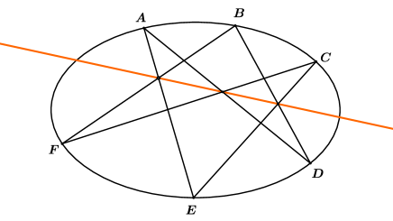
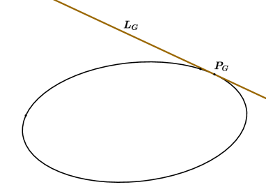
The line containing them is called the Pascal line, or just the Pascal, of the array; we will denote it by $\left\{\begin{array}[]{ccc}A&B&C\\ F&E&D\end{array}\right\}$. It is easy to see that the Pascal remains unchanged if we permute the rows or the columns of the array; thus

$$\left\{\begin{array}[]{ccc}A&B&C\\ F&E&D\end{array}\right\},\quad\left\{\begin{array}[]{ccc}F&E&D\\ A&B&C\end{array}\right\},\quad\left\{\begin{array}[]{ccc}E&D&F\\ B&C&A\end{array}\right\}$$ (1.1)

all denote the same line.

Any essentially different arrangement of the same points, say $\left\{\begin{array}[]{ccc}E&A&C\\ B&F&D\end{array}\right\}$, corresponds a priori to a different line. Hence we have a total of $\frac{6!}{2!3!}=60$ notionally distinct Pascals. It is a theorem due to Pedoe [12], that these $60$ lines are distinct if the initial six points are chosen generally.222If one tries to draw a diagram of the sextuple together with all sixty of its Pascals, a dense and incomprehensible profusion of ink is the usual outcome. The curious reader is referred to http://mathworld.wolfram.com/PascalLines.html The configuration of six points with all of its associated lines is sometimes called Pascal’s hexagram.

The best classical references for the geometry of Pascal lines are by Salmon [14, Notes] and Baker [2, Note II, pp. 219–236]. An engaging recent account is given in the article by Conway and Ryba [5]. The reader is referred to [9] and [16] for standard facts about projective planes.

1.2.

It is natural to wonder to what extent the construction sequence

$$\text{six points on $\mathcal{K}$}\leadsto\text{sixty lines in the plane}$$

can be reversed; that is to say, whether one can reconstruct the initial sextuple if the positions of some of the Pascals are known.333The conic itself is fixed throughout, and as such assumed to be known. In this paper we establish the following result:

The Main Theorem (Preliminary Form).

The sextuple $A,\dots,F$ can be reconstructed from the following four Pascals:

$$\ell_{1}=\left\{\begin{array}[]{ccc}A&D&B\\ E&C&F\end{array}\right\},\quad\ell_{2}=\left\{\begin{array}[]{ccc}A&C&F\\ E&D&B\end{array}\right\},\quad\ell_{3}=\left\{\begin{array}[]{ccc}A&D&F\\ E&C&B\end{array}\right\},\quad\ell_{\star}=\left\{\begin{array}[]{ccc}A&B&C\\ F&D&E\end{array}\right\}.$$ (1.2)

The arrays follow a pattern and the last one is on a different footing from the first three; this will be explained in section 1.4.

1.3.

In order to state the theorem more precisely, let $[z_{0},z_{1},z_{2}]$ be the homogeneous coordinates on $\mathbf{P}^{2}$, and let the conic $\mathcal{K}$ be defined by the equation $z_{1}^{2}=z_{0}\,z_{2}$. Lines in $\mathbf{P}^{2}$ are also given by homogeneous coordinates; for instance, the line $2\,z_{0}+3\,z_{1}+5\,z_{2}=0$ has line coordinates $\langle 2,3,5\rangle$.

Choose independent variables $a,\dots,f$, and fix the points

$$A=[1,a,a^{2}],\quad B=[1,b,b^{2}],\quad\dots,F=[1,f,f^{2}]$$ (1.3)

on $\mathcal{K}$.

Let $\langle 1,s_{i},t_{i}\rangle$ denote the line coordinates of $\ell_{i}$ for $i=1,2,3$, and $\langle 1,s_{*},t_{*}\rangle$ those of $\ell_{*}$. Each of these Pascals is obtained by starting from the points in (1.3) and taking joins and intersections, hence it is intuitively clear that $s_{i}$ and $t_{i}$ are rational functions in $a,\dots,f$. The actual expressions are rather cumbersome; for instance,

$$s_{1}=\frac{abf-abe-acd+\text{$9$ similar terms}}{abce-abcf+\text{$4$ similar terms}},\quad t_{1}=\frac{ac-af-bc+\text{$3$ similar terms}}{abce-abcf+\text{$4$ similar terms}},$$ (1.4)

and likewise for the other $s_{i},t_{i}$. The reconstruction problem is to go backwards from the collection of Pascals $\{\ell_{1},\ell_{2},\ell_{3},\ell_{*}\}$ to the collection of points $\{A,\dots,F\}$. Our result says that this can be done in algebraically the simplest possible way.

The Main Theorem (Refined Form).

Each of the variables $a,\dots,f$ can be expressed as a rational function of $s_{i}$ and $t_{i}$ for $i=1,2,3,*$.

A naive attempt to prove the theorem would start from the formulae for $s_{1},\dots,t_{*}$, and try to ‘solve’ for the variables $a,\dots,f$. However, the expressions in (1.4) are too complicated for this to succeed. We will instead use binary quadratic forms to represent points and lines in $\mathbf{P}^{2}$, and express their joins and intersections in the language of transvectants (see section 2). One can then make these rational functions completely explicit by exploiting the geometry of the Pascals in conjunction with the graphical calculus for binary forms. It is an immediate corollary of the main theorem that the Galois group of Pascal lines is isomorphic to the symmetric group $\mathfrak{S}_{6}$.

Our main theorem is thematically similar to, and partly inspired by, Wernick’s problems in Euclidean triangle geometry - more on this in section 1.5 below.

1.4. An overview of the proof

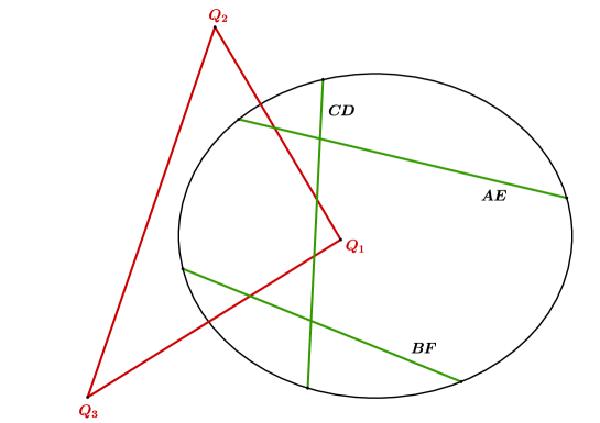
The relevant geometric elements are shown in Diagram 2 on page 2. Since each Pascal corresponds to a $2\times 3$ array (determined up to a shuffling of rows and columns), its columns give a partition of the points $A,\dots,F$ into three sets of two elements each. For instance, any of the arrays in (1.1) gives the partition

$$\{A,F\}\cup\{B,E\}\cup\{C,D\}.$$

Now observe that the first three Pascals in (1.2) have been so chosen that they all lead to the same partition, namely

$$\{A,E\}\cup\{C,D\}\cup\{B,F\}.$$ (1.5)

This corresponds to the three green chords in Diagram 2. Let $Q_{1}$ denote the point $AB\cap EF$, which is common to $\ell_{2}$ and $\ell_{3}$. Similarly, let

$$Q_{2}=\ell_{3}\cap\ell_{1}=AC\cap DE,\qquad Q_{3}=\ell_{1}\cap\ell_{2}=BC\cap DF.$$ (1.6)

Hence the line $Q_{1}Q_{2}$ is the same as $\ell_{3}$, and so on. Now, if we switch the endpoints of all the three chords simultaneously; that is to say, if we apply the transposition

$$(A\,E)\,(C\,D)\,(B\,F),$$

then all the $Q_{i}$ remain unchanged and hence so do the first three Pascals. In other words, each of the expressions $s_{1},t_{1},\dots,s_{3},t_{3}$ remains invariant if we make a simultaneous substitution of variables $a\leftrightarrow e,c\leftrightarrow d,b\leftrightarrow f$. It follows that no rational function of $s_{1},\dots,t_{3}$ can equal any of the variables $a,\dots,f$.

The first stage in the proof is to show that the next best outcome is achievable; that is to say, the symmetric expressions

$$a+e,\quad a\,e,\quad b+f,\quad b\,f,\quad c+d,\quad c\,d$$

are rational functions of $s_{1},\dots,t_{3}$. In geometric terms (see the top part of Diagram 2), the red triangle $Q_{1}Q_{2}Q_{3}$ allows us to locate the three green chords, but we do not yet have sufficient information to label their endpoints. The algebraic formulae which connect the red triangle to the green chords are encoded in a transvectant identity.

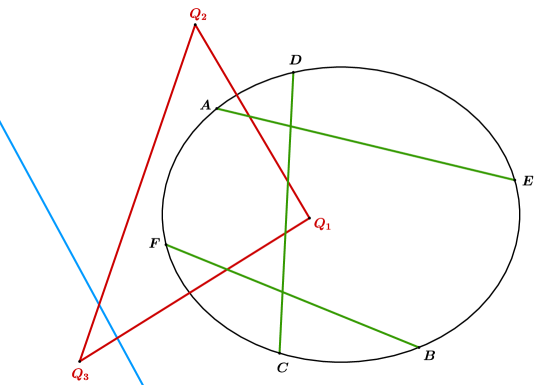
In the second stage, we bring in the fourth Pascal $\ell_{*}$ (shown in blue) to break the symmetry. It is so chosen that each of the three green chords passes through one of the cross-hair intersections in $\ell_{*}$; for instance, $BF$ passes through the point $AD\cap BF$ on $\ell_{*}$. And now, another transvectant identity allows us to get a linear equation for $a$ whose coefficients are rational functions in $s_{1},\dots,t_{*}$. This implies that $a$ itself is such a function, and a similar argument applies to $b,\dots,f$. This gives the required result.

Refer to caption
Refer to caption
Diagram 2. Dramatis Personae in the reconstruction

1.5. Wernick’s Problems

As an aside, we will point out the analogy between the reconstruction problem for Pascals and Wernick’s problems [15, 17]. Given a triangle $ABC$ in the Euclidean plane, one gets a large number of derived points such as the centroid, the orthocentre or the three foots of perpendiculars. A typical Wernick’s problem asks whether the original triangle can be reconstructed from a specific choice of three of the derived points. Here are two sample results (see [15, p. 71]):

  • Given the centroid, orthocentre and the midpoint of any one side, the original triangle is constructible.

  • The original triangle is not constructible from the circumcentre, orthocentre and the incentre.

It is clear that our main theorem is in this spirit, although the specific geometric situation is different. The coordinates of any of the derived points are often given by simple formulae in terms of the coordinates of $A,B,C$. The analogous formulae (1.4) in our case are more involved, and hence the reconstruction is less straightforward.

2. Binary forms

2.1.

Let $\mathcal{E}$ denote the field $\mathbf{Q}(a,b,c,d,e,f)$ of rational functions in the variables $a,\dots,f$. We will use $\mathcal{E}$ as our base field, so that any ‘scalar’ will be assumed to belong to $\mathcal{E}$. Henceforth, the projective plane $\mathbf{P}^{2}$ will be over $\mathcal{E}$.

We will consider homogeneous forms in the variables $\mathbf{x}=\{x_{1},x_{2}\}$. In a classical notation introduced by Cayley, $(z_{0},z_{1},\dots,z_{n})(x_{1},x_{2})^{n}$ stands for the degree $n$ form $\sum\limits_{i=0}^{n}\,z_{i}\,\binom{n}{i}\,x_{1}^{n-i}\,x_{2}^{i}$.

2.2. Transvectants

Although the definition of a transvectant is prima facie technical, the concept arises naturally in invariant theory and representation theory (see [11, Ch. 5]).

Suppose that we are given two binary forms $G,H$ of degrees $m,n$ respectively. For an integer $r\geqslant 0$, their $r$-th transvectant is defined to be

$$(G,H)_{r}=\frac{(m-r)!\,(n-r)!}{m!\,n!}\,\sum\limits_{i=0}^{r}\,(-1)^{i}\binom{r}{i}\,\frac{\partial^{r}G}{\partial x_{1}^{r-i}\,\partial x_{2}^{i}}\,\frac{\partial^{r}H}{\partial x_{1}^{i}\,\partial x_{2}^{r-i}}$$ (2.1)

This is a form of degree $m+n-2r$, unless it is identically zero. If

$$G=(g_{0},g_{1},g_{2})(x_{1},x_{2})^{2},\quad H=(h_{0},h_{1},h_{2})(x_{1},x_{2})^{2},$$

then it is easy to check that

$\displaystyle(G,H)_{1}$ $\displaystyle=(g_{0}h_{1}-g_{1}h_{0},\frac{1}{2}\,(g_{0}\,h_{2}-g_{2}\,h_{0}),g_{1}\,h_{2}-g_{2}\,h_{1})(x_{1},x_{2})^{2},\;\text{and}$
$\displaystyle(G,H)_{2}$ $\displaystyle=g_{0}h_{2}-2\,g_{1}h_{1}+g_{2}h_{0}.$

In general, the coefficients of $(G,H)_{r}$ are linear functions in the coefficients of $G$ and $H$. The numerical factors in Cayley’s notation and (2.1) may seem unnecessary, but experience has shown that they simplify the computations.

2.3.

Now the crucial step is to represent points and lines in $\mathbf{P}^{2}$ by quadratic binary forms. (The reader may also refer to [3, §3] where an identical set-up is used.) Let the nonzero quadratic form $G=(g_{0},g_{1},g_{2})(x_{1},x_{2})^{2}$ represent the point $P_{G}=[g_{0},g_{1},g_{2}]$, as well as the line $L_{G}=\langle g_{2},-2\,g_{1},g_{0}\rangle$. It is understood that any nonzero scalar multiple of $G$ will represent the same point or line. Now the following properties show that incidences and joins are exactly mirrored by transvectants.

Lemma 2.1.

With notation as above,

  1. (1)

    The point $P_{G}$ belongs to the line $L_{H}$, if and only if $(G,H)_{2}=0$.

  2. (2)

    The line joining the points $P_{G}$ and $P_{H}$ is $L_{(G,H)_{1}}$.

  3. (3)

    The point of intersection of the lines $L_{G}$ and $L_{H}$ is $P_{(G,H)_{1}}$.

All the proofs follow immediately from the definitions. The point $P_{G}=[g_{0},g_{1},g_{2}]$ lies on $L_{H}=\langle h_{2},-2\,h_{1},h_{0}\rangle$ exactly when the dot product of the two vectors is zero, which proves (1). The equation of the line joining $P_{G}$ and $P_{H}$ is $\left|\begin{array}[]{ccc}z_{0}&z_{1}&z_{2}\\ g_{0}&g_{1}&g_{2}\\ h_{0}&h_{1}&h_{2}\end{array}\right|=0$, hence it is represented by $(G,H)_{1}$. The proof of (3) is similar. ∎

The following result will be needed later.

Lemma 2.2.

Two nonzero quadratic forms $G$ and $H$ are equal up to a scalar, if and only if $(G,H)_{1}=0$.

Proof.

The forms are equal up to a scalar exactly when the matrix $\left[\begin{array}[]{ccc}g_{0}&g_{1}&g_{2}\\ h_{0}&h_{1}&h_{2}\end{array}\right]$ has rank one, i.e., exactly when all of its minors are zero. This is equivalent to the vanishing of all the coefficients of $(G,H)_{1}$. ∎

The advantage of using transvectants is that there are well-developed tools for manipulating them, namely, a symbolic calculus (see [6, 11]) as well as a graphical calculus (see [1, §2]). This is especially useful when one encounters transvectants whose components are themselves transvectants.

2.4.

The conic $\mathcal{K}$ consists of those points $P_{G}$ such that

$$(G,G)_{2}=2\,(g_{1}^{2}-g_{0}\,g_{2})=0.$$

These are the nonzero forms $G$ which can be written as squares of linear forms up to a scalar. Define six linear forms

$$a_{\mathbf{x}}=x_{1}+a\,x_{2},\quad b_{\mathbf{x}}=x_{1}+b\,x_{2},\quad\dots\quad f_{\mathbf{x}}=x_{1}+f\,x_{2},$$

and fix the points $A=P_{a_{\mathbf{x}}^{2}},\dots,F=P_{f_{\mathbf{x}}^{2}}$ on $\mathcal{K}$. Let

$$\lambda_{i}=(t_{i},-\frac{s_{i}}{2},1)(x_{1},x_{2})^{2},\qquad i=1,2,3,*$$ (2.2)

denote the quadratic forms which represent the Pascals $\ell_{i}$. All of this agrees with the notational conventions in section 1.3.

The following lemma is helpful in completing the geometric picture, but it will not be needed elsewhere (see Diagram 3).
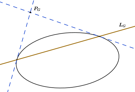
Refer to caption
Refer to caption
Diagram 3. The pole-polar relation
Lemma 2.3.

Let $G$ denote a nonzero quadratic form. Then $L_{G}$ is the polar line of $P_{G}$ with respect to $\mathcal{K}$. In particular,

$$\text{$P_{G}$ lies on $L_{G}$}\iff\text{$P_{G}$ lies on $\mathcal{K}$}\iff\text{$L_{G}$ is tangent to $\mathcal{K}$}.$$

The proof is left to the reader. ∎

2.5.

For instance, the line $AB$ is represented by the form $(a_{\mathbf{x}}^{2},b_{\mathbf{x}}^{2})_{1}=(b-a)\,a_{\mathbf{x}}\,b_{\mathbf{x}}$, or after ignoring the scalar, just by $a_{\mathbf{x}}\,b_{\mathbf{x}}$. It follows that the points $Q_{1},Q_{2},Q_{3}$ in section 1.4 are respectively represented by the quadratic forms

$$\pi_{1}=(a_{\mathbf{x}}b_{\mathbf{x}},e_{\mathbf{x}}f_{\mathbf{x}})_{1},\quad\pi_{2}=(a_{\mathbf{x}}c_{\mathbf{x}},d_{\mathbf{x}}e_{\mathbf{x}})_{1},\quad\pi_{3}=(b_{\mathbf{x}}c_{\mathbf{x}},d_{\mathbf{x}}f_{\mathbf{x}})_{1}.$$ (2.3)

Since $Q_{1}=\ell_{2}\cap\ell_{3}$ etc, they are also respectively represented by

$$\mu_{1}=(\lambda_{2},\lambda_{3})_{1},\quad\mu_{2}=(\lambda_{3},\lambda_{1})_{1},\quad\mu_{3}=(\lambda_{1},\lambda_{2})_{1}.$$ (2.4)

This implies that $\mu_{i}$ and $\pi_{i}$ are equal up to a multiplicative scalar in $\mathcal{E}$. It is clear that the coefficients of $\mu_{i}$ are rational functions in $s_{1},\dots,t_{3}$.

3. The proof of the main theorem

3.1. The first stage

For any quadratic forms $U,V,W$, define

$$\psi(U,V,W)=6\,(U,VW)_{2}-U(V,W)_{2},$$

which is also a quadratic form.

Proposition 3.1.

We have an identity

$$\psi(\pi_{3},\pi_{1},\pi_{2})=\Phi\times a_{\mathbf{x}}\,e_{\mathbf{x}},$$ (3.1)

where $\Phi$ is a polynomial in $a,\dots,f$.

The proof will be given in section 4 using the graphical calculus, but the rationale behind the proposition can be explained without it. The right-hand side of (3.1) represents the line $AE$. Since $\mu_{i}$ is proportional to $\pi_{i}$, the left-hand side is proportional to $\psi(\mu_{3},\mu_{1},\mu_{2})$. Hence the identity implies that $AE$ can be represented by a form

$$\lambda_{AE}=(\alpha_{AE},\beta_{AE},1)(x_{1},x_{2})^{2},$$

where $\alpha_{AE},\beta_{AE}$ are rational functions of $s_{1},\dots,t_{3}$. We can similarly write down $\lambda_{CD}$ and $\lambda_{BF}$ representing the other two green chords in Diagram 2. The exact expression for $\Phi$ will be found in the course of proving the identity, but it is immaterial to the main theorem.

Formula (3.1) was initially obtained by some calculated guesswork guided by intuition. Since the construction of Pascals is synthetic, if it is at all possible to pass from the red triangle to the green chords, then the connecting formula can be plausibly written in terms of transvectants. Since the letters $a,e$ enter symmetrically into the expressions for $\pi_{1},\pi_{2}$, the formula should respect this structure as well. Now the correct definition of $\psi$ is determined by a graphical calculation, in which the initial intuition is buttressed by a formal proof.

A direct calculation shows that

$$\alpha_{AE}=\frac{s_{1}^{2}\,s_{3}\,t_{2}\,t_{3}-s_{1}^{2}\,s_{2}\,t_{3}^{2}+\text{$16$ similar terms}}{s_{1}^{2}\,s_{2}\,t_{2}+s_{1}\,s_{2}\,s_{3}\,t_{1}+\text{$16$ similar terms}},$$

with a similar expression for $\beta_{AE}$. Thus (3.1) serves as a compact shorthand for a lengthy and complicated formula.

3.2. The second stage

We now use the fourth Pascal $\ell_{*}$. Recall that a point on $\mathcal{K}$ is represented by the square of a linear form which is well-defined up to a scalar. Thus $A$ comes from $a_{\mathbf{x}}$, where we are hoping to solve for $a$ in terms of $s_{1},t_{1},\dots,s_{*},t_{*}$. There are two ways of expressing $D$ in terms of $A$, and their comparison will lead to a set of equations for $a$.

Refer to caption
Diagram 4. The double dependence of $D$ on $A$

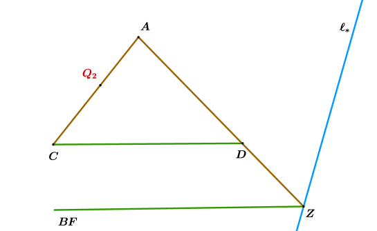
Diagram 4 shows the geometric elements needed in the second step.

  1. (1)

    Since the point $Q_{2}$ is on $AC$, the line $AQ_{2}$ is the same as $AC$. Now $AQ_{2}$ is represented by

    $$(\mu_{2},a_{\mathbf{x}}^{2})_{1}=a_{\mathbf{x}}\,(\mu_{2},a_{\mathbf{x}})_{1}.$$

    Hence $C$ comes from the linear form $(\mu_{2},a_{\mathbf{x}})_{1}$, and thus $D$ comes from

    $$\frac{\lambda_{CD}}{(\mu_{2},a_{\mathbf{x}})_{1}}.$$ (3.2)
  2. (2)

    The Pascal $\ell_{*}$ passes through $Z=AD\cap BF$, which implies that $Z$ is represented by $(\ell_{\star},\lambda_{BF})_{1}$. Hence $AZ$, which is the same as $AD$, is represented by

    $$((\ell_{*},\lambda_{BF})_{1},a_{\mathbf{x}}^{2})_{1}=a_{\mathbf{x}}\,((\ell_{*},\lambda_{BF})_{1},a_{\mathbf{x}})_{1}.$$

    Thus $D$ also comes from

    $$((\ell_{*},\lambda_{BF})_{1},a_{\mathbf{x}})_{1}.$$ (3.3)

The two linear forms in (3.2) and (3.3) must coincide up to a scalar. This gives the identity

$$\lambda_{CD}=\text{scalar}\times(\mu_{2},a_{\mathbf{x}})_{1}\,\times((\ell_{*},\lambda_{BF})_{1},a_{\mathbf{x}})_{1}.$$

If we write

$$U=\lambda_{CD},\quad V=\mu_{2},\quad W=(\ell_{*},\lambda_{BF})_{1},$$

then, by Lemma 2.2, this is equivalent to

$$(U,(V,a_{\mathbf{x}})_{1}\,(W,a_{\mathbf{x}})_{1})_{1}=0.$$

The following transvectant identity allows us to rewrite this in such a way that we can extract a set of equations for $a$.

Proposition 3.2.

For arbitrary quadratic forms $U,V,W$ and linear form $a_{\mathbf{x}}$, we have an identity

$$(U,(V,a_{\mathbf{x}})_{1}\,(W,a_{\mathbf{x}})_{1})_{1}=(M,a_{\mathbf{x}}^{2})_{2}+(N,a_{\mathbf{x}}^{2})_{1},$$ (3.4)

where

$$M=\frac{1}{2}\,(U,W)_{1}\,V+\frac{1}{2}\,(U,V)_{1}\,W,\qquad N=-\frac{1}{2}\,(U,VW)_{2}-\frac{1}{6}\,U(V,W)_{2}.$$

The proof will be given in section 4. The purpose of the identity is to ‘package’ the known quantities $U,V,W$ into $M$ and $N$, so as to separate them from the unknown quantity $a$.

3.3.

Now write

$$M=(m_{0},m_{1},m_{2},m_{3},m_{4})(x_{1},x_{2})^{4},\quad\text{and}\quad N=(n_{0},n_{1},n_{2})((x_{1},x_{2})^{2}.$$

The coefficients of $U,V,W$ are rational functions of $s_{1},\dots,t_{*}$, hence so are all the $m_{i}$ and $n_{i}$. The right-hand side of (3.4) can be expanded as $(r_{0},r_{1},r_{2})(x_{1},x_{2})^{2}$, where each $r_{i}$ is quadratic in $a$. Since this must vanish identically, we get three quadratic equations $r_{0}=r_{1}=r_{2}=0$ for $a$. A straightforward expansion shows that they can be written as

$$\left[\begin{array}[]{ccc}m_{2}-n_{1}&n_{0}-2\,m_{1}&m_{0}\\ 2\,m_{3}-n_{2}&-4\,m_{2}&2\,m_{1}+n_{0}\\ m_{4}&-2\,m_{3}-n_{2}&m_{2}+n_{1}\end{array}\right]\left[\begin{array}[]{c}1\\ a\\ a^{2}\end{array}\right]=0.$$

Let $Z=(z_{ij})$ denote the $3\times 3$ matrix on the left; e.g., $z_{12}=n_{0}-2m_{1}$. Now, for instance, we can use its first two rows to solve for $a$, which gives

$$a=-\frac{\left|\begin{array}[]{cc}z_{11}&z_{13}\\ z_{21}&z_{23}\end{array}\right|}{\left|\begin{array}[]{cc}z_{12}&z_{13}\\ z_{22}&z_{23}\end{array}\right|}.$$

This proves that $a$ is a rational function of $s_{1},\dots,t_{*}$. Since $e_{\mathbf{x}}$ is a constant multiple of $\frac{\lambda_{AE}}{a_{\mathbf{x}}}$, the same follows for $e$. The Pascal $\ell_{*}$ passes through the points $CD\cap BE,AE\cap CF$ which respectively lie on the green chords $CD,AE$. Hence the same argument as in the second stage gives the result for $b,c,d,f$. This proves the main theorem, assuming Propositions 3.1 and 3.2. ∎

The passage

$$\{s_{1},t_{1},\dots,s_{*},t_{*}\}\Rightarrow\{a,\dots,f\}$$

goes through two complicated algebraic identities neither of which has any obvious geometric content. Thus our reconstruction is not ‘synthetic’ in the classical sense of the word. We do not know of any natural ruler-and-compass type construction which begins with the Pascals and ends with the sextuple. It would be interesting to find one.

3.4.

The main theorem is valid over any field of characteristic zero, since the choice of $\mathbf{Q}$ plays no essential role in the proof. Moreover, the only numerical coefficients which appear in the proof are $2,4,6$ and $\frac{3}{4}$. All of these are defined and nonzero as long as the base field has characteristic $\neq 2,3$, and hence the theorem remains valid over such a field. It would be interesting to have a similar theorem when the characteristic is either $2$ or $3$.

3.5.

We have programmed the entire procedure in Maple in order to ensure against the possibility of error. For instance, suppose that

$$a=7,\quad b=-3,\quad c=2,\quad d=5,\quad e=-4,\quad f=1.$$

Then the Pascals are

$$\begin{array}[]{lll}\lambda_{1}=(\frac{5}{36},\frac{37}{72},1)(x_{1},x_{2})^{2},&&\lambda_{2}=(-\frac{49}{349},\frac{42}{349},1)(x_{1},x_{2})^{2},\\ \lambda_{3}=(-\frac{1}{16},-\frac{33}{544},1)(x_{1},x_{2})^{2},&&\lambda_{*}=(\frac{7}{74},\frac{21}{148},1)(x_{1},x_{2})^{2}.\end{array}$$

Now if we follow the recipe given above, the result is

$$a=\frac{5^{7}.7^{2}.11^{12}.13^{4}.29^{14}}{5^{7}.7.11^{12}.13^{4}.29^{14}}=7$$

as expected, and similarly for the remaining variables. We have done a similar verification on several such examples.

3.6.

The theme of this paper is related to the Galois (or monodromy) group of Pascal lines in the sense of [7]. We explain this in brief.

Assume the base field to be $\mathbf{C}$. Write

$$(T-a)\,(T-b)\,\dots(T-f)=T^{6}-s_{1}\,T^{5}+s_{2}\,T^{4}-s_{3}\,T^{3}+s_{4}\,T^{2}-s_{5}\,T+s_{6},$$

where $s_{1},\dots,s_{6}$ are the elementary symmetric functions in $a,\dots,f$. Let $\mathcal{Z}$ denote the space of unordered six points on a conic. In fact $\mathcal{Z}$ is birational to $\text{Sym}^{6}\mathcal{K}\simeq\mathbf{P}^{6}$, and its field of rational functions may be identified with

$$\mathcal{F}=\mathbf{C}(s_{1},\dots,s_{6}).$$

We have a $60$-$1$ cover $\mathcal{Y}\longrightarrow\mathcal{Z}$, where the fibre over an unordered sextuple corresponds to its collection of $60$ Pascals. If $\langle 1,s_{i},t_{i}\rangle,1\leqslant i\leqslant 60$ are the line coordinates of the Pascals, then the field of rational functions of $\mathcal{Y}$ is $\mathcal{F}(s_{1},t_{1},\dots,s_{60},t_{60})$. However, the inclusion

$$\mathcal{F}(s_{1},t_{1},\dots,s_{60},t_{60})\subseteq\mathbf{C}(a,\dots,f)$$ (3.5)

is actually an equality by our main theorem. Hence we have the following:

Proposition 3.3.

The Galois group

$$\text{Gal}(\mathcal{Y}/\mathcal{Z})\simeq\text{Gal}(\mathbf{C}(a,\dots,f)/\mathbf{C}(s_{1},\dots,s_{6}))$$

is isomorphic to the symmetric group on six letters.

It should be clarified that this result cannot be considered original to this paper. The fact that (3.5) is an equality is already implicit in Pedoe’s proof in [12], although it is not so stated there.

3.7. Optimal subsets

Let $X$ be an arbitrary $n$-element subset of the sixty Pascals, with line coordinates

$$\langle 1,s^{(i)},t^{(i)}\rangle,\quad 1\leqslant i\leqslant n.$$

This gives an inclusion of fields

$$\underbrace{\mathbf{Q}(s^{(1)},t^{(1)},\dots,s^{(n)},t^{(n)})}_{\mathcal{E}_{X}}\subseteq\mathcal{E}.$$ (3.6)

Let us say that the set $X$ is adequate if equality holds; this is equivalent to saying that each variable is a rational function in $s^{(1)},\dots,t^{(n)}$. Furthermore, let us say that $X$ is optimal if it is adequate and no proper subset of $X$ is adequate.

Proposition 3.4.

The set of Pascals given in the main theorem is optimal.

Proof.

It is clear that $\{\ell_{1},\ell_{2},\ell_{3}\}$ is not adequate, in fact (3.6) is a quadratic extension in this case. If we take $X=\{\ell_{1},\ell_{2},\ell_{*}\}$, then a Maple computation shows that (3.6) is a degree $12$ extension, and hence $X$ is not adequate. (It would be better to have a more conceptual and less computational proof, but we cannot find one.)

Now observe that the permutation $(A\,F)\,(B\,E)\,(C\,D)$ leaves $\ell_{1},\ell_{*}$ unchanged, and interchanges $\ell_{2}$ and $\ell_{3}$. Hence the same result follows for $\{\ell_{1},\ell_{3},\ell_{*}\}$. Finally, the permutation $(A\,D)\,(B\,F)\,(C\,E)$ interchanges $\ell_{1},\ell_{3}$ and leaves $\ell_{2},\ell_{*}$ unchanged, which proves that $\{\ell_{2},\ell_{3},\ell_{*}\}$ is not adequate. This completes the proof. ∎

Since $\mathcal{E}$ has transcendence degree $6$ over $\mathbf{Q}$, any adequate subset must have at least $3$ elements. It would be of interest to know whether there exists an adequate $3$-element subset, which must then be necessarily optimal. We have not succeeded in finding any.

On the other hand, given an arbitrary subset of (three or more) Pascals, it is not at all obvious how to decide whether it is adequate. Thus there is a large number of Wernick-Pascal type reconstruction problems which remain open. It is a matter of speculation whether transvectant identities of some sort will play a role in their solution.

3.8.

There are geometric obstructions which prevent certain sets from being adequate. Consider the set $X$ consisting of Pascals

$$\left\{\begin{array}[]{ccc}A&B&C\\ F&E&D\end{array}\right\},\quad\left\{\begin{array}[]{ccc}A&B&C\\ D&F&E\end{array}\right\},\quad\left\{\begin{array}[]{ccc}A&B&C\\ E&D&F\end{array}\right\},$$

where the top row is held constant and the bottom row undergoes a cyclic shift. Steiner’s theorem says that these three Pascals are concurrent. If $\langle 1,s^{(i)},t^{(i)}\rangle,i=1,2,3$ denote their line coordinates, then the determinant $\left|\begin{array}[]{ccc}1&s^{(1)}&t^{(1)}\\ 1&s^{(2)}&t^{(2)}\\ 1&s^{(3)}&t^{(3)}\end{array}\right|=0$. Hence $\mathcal{E}_{X}$ has transcendence degree at most $5$ over444It can be shown to be exactly $5$, but this is not needed for the conclusion. $\mathbf{Q}$, and $X$ cannot be adequate. Rather similarly, Kirkman’s theorem says that the Pascals

$$\left\{\begin{array}[]{ccc}A&B&C\\ F&E&D\end{array}\right\},\quad\left\{\begin{array}[]{ccc}A&D&F\\ C&E&B\end{array}\right\},\quad\left\{\begin{array}[]{ccc}A&C&F\\ E&B&D\end{array}\right\},$$

are concurrent, and then the same conclusion follows. The reader will find a proof of either theorem in Salmon’s notes referred to above.

4. Transvectant identities

In this section we will prove Propositions 3.1 and 3.2. The proofs rely upon the graphical formalism555It has a close affinity to the classical symbolic calculus as practiced by the German school of invariant theorists in the nineteenth century (cf. [4, 6, 10]). The bibliography of [1] contains several more references to this circle of ideas. developed in [1, §2].

4.1.

We will first rewrite Proposition 3.1 in more general and precise form. Consider six general linear forms $a_{\mathbf{x}}=a_{1}x_{1}+a_{2}x_{2}$, $b_{\mathbf{x}}=b_{1}x_{1}+b_{2}x_{2}$, …, $f_{\mathbf{x}}=f_{1}x_{1}+f_{2}x_{2}$, where a letter such as ‘$a$’ stands for a pair of variables $(a_{1},a_{2})$ instead of a single one. We will also use the classical bracket notation $(ab)=a_{1}b_{2}-a_{2}b_{1}$ for $2\times 2$ determinants, and similarly for $(cd)$, $(bf)$, etc.

Write

$$U=(b_{\mathbf{x}}c_{\mathbf{x}},d_{\mathbf{x}}f_{\mathbf{x}})_{1},\quad V=(a_{\mathbf{x}}c_{\mathbf{x}},d_{\mathbf{x}}e_{\mathbf{x}})_{1},\quad W=(a_{\mathbf{x}}b_{\mathbf{x}},e_{\mathbf{x}}f_{\mathbf{x}})_{1},$$

and $\psi(U,V,W)=6(U,VW)_{2}-U(V,W)_{2}$. Define

$$\mathcal{S}=(da)(fc)(eb)-(ce)(bd)(af).$$ (4.1)
Proposition 4.1.

With notation as above, we have

$$\psi(U,V,W)=\Phi\ a_{\mathbf{x}}e_{\mathbf{x}},$$

where $\Phi=\frac{3}{4}(cd)(bf)\ \mathcal{S}$.

Remark 4.2.

The expression $\mathcal{S}$ has the following invariance property. Let $J$ denote the operation of making a simultaneous exchange of letters $a\leftrightarrow b,e\leftrightarrow f$. Now $\mathcal{S}$ remains invariant under the action of $J$, since the bracket factors $(da),(fc),(eb)$ are respectively taken to $(db),(ec),(fa)$ and conversely. Similarly, let $K$ and $L$ respectively denote the operations

$$b\leftrightarrow c,f\leftrightarrow d,\quad\text{and}\quad a\leftrightarrow e,b\leftrightarrow f,c\leftrightarrow d.$$

Then $K$ also leaves $\mathcal{S}$ invariant, whereas $L$ changes it to $-\mathcal{S}$. The subgroup generated by $J,K$ and $L$ inside the permutation group on letters $a,\dots,f$, is isomorphic to $\mathfrak{S}_{3}\times\mathbf{Z}_{2}$.

Lemma 4.3.

We have the more symmetric rewriting

$$\psi(U,V,W)=3\left[(U,V)_{2}W+(U,W)_{2}V-(V,W)_{2}U\right]\ .$$
Proof.

Using the graphical formalism of [1, §2], we can write

(U,VW)2=\psfrag{U}{$\scriptstyle{U}$}\psfrag{V}{$\scriptstyle{V}$}\psfrag{W}{$\scriptstyle{W}$}\psfrag{x}{$\scriptstyle{x}$}\includegraphics[width=62.59596pt]{pic1.eps}=14![4(U,V)2W+4(U,W)2V+16\psfrag{U}{$\scriptstyle{U}$}\psfrag{V}{$\scriptstyle{V}$}\psfrag{W}{$\scriptstyle{W}$}\psfrag{x}{$\scriptstyle{x}$}\includegraphics[width=71.13188pt]{pic2.eps}](U,VW)_{2}=\ \ \parbox{62.59596pt}{ \includegraphics[width=62.59596pt]{pic1.eps}}\ \ =\frac{1}{4!}\left[4(U,V)_{2}W+4(U,W)_{2}V+16\ \ \parbox{71.13188pt}{ \includegraphics[width=71.13188pt]{pic2.eps}}\ \ \right] (4.2)

by expanding the normalized $\mathfrak{S}_{4}$ symmetrizer (represented by the grey rectangle). We will use the notation

{VUW}=\psfrag{U}{$\scriptstyle{U}$}\psfrag{V}{$\scriptstyle{V}$}\psfrag{W}{$\scriptstyle{W}$}\psfrag{x}{$\scriptstyle{x}$}\includegraphics[width=71.13188pt]{pic2.eps}.𝑉𝑈𝑊\psfrag{U}{$\scriptstyle{U}$}\psfrag{V}{$\scriptstyle{V}$}\psfrag{W}{$\scriptstyle{W}$}\psfrag{x}{$\scriptstyle{x}$}\includegraphics[width=71.13188pt]{pic2.eps}\{V\rightarrow U\leftarrow W\}=\ \parbox{71.13188pt}{ \includegraphics[width=71.13188pt]{pic2.eps}}\ \ .

Inserting the matrix identity $\epsilon\epsilon^{\rm T}=I$ (where $\epsilon$ is the $2\times 2$ antisymmetric matrix with $\epsilon_{12}=1$ represented by the arrows), and using the Grassmann-Plücker (GP) relation where indicated by the dotted line, we have

{VUW}=\psfrag{U}{$\scriptstyle{U}$}\psfrag{V}{$\scriptstyle{V}$}\psfrag{W}{$\scriptstyle{W}$}\psfrag{x}{$\scriptstyle{x}$}\psfrag{G}{$\scriptstyle{GP}$}\includegraphics[width=71.13188pt]{pic3.eps}=\psfrag{U}{$\scriptstyle{U}$}\psfrag{V}{$\scriptstyle{V}$}\psfrag{W}{$\scriptstyle{W}$}\psfrag{x}{$\scriptstyle{x}$}\includegraphics[width=71.13188pt]{pic4.eps}\psfrag{U}{$\scriptstyle{U}$}\psfrag{V}{$\scriptstyle{V}$}\psfrag{W}{$\scriptstyle{W}$}\psfrag{x}{$\scriptstyle{x}$}\includegraphics[width=71.13188pt]{pic5.eps},𝑉𝑈𝑊\psfrag{U}{$\scriptstyle{U}$}\psfrag{V}{$\scriptstyle{V}$}\psfrag{W}{$\scriptstyle{W}$}\psfrag{x}{$\scriptstyle{x}$}\psfrag{G}{$\scriptstyle{GP}$}\includegraphics[width=71.13188pt]{pic3.eps}\psfrag{U}{$\scriptstyle{U}$}\psfrag{V}{$\scriptstyle{V}$}\psfrag{W}{$\scriptstyle{W}$}\psfrag{x}{$\scriptstyle{x}$}\includegraphics[width=71.13188pt]{pic4.eps}\psfrag{U}{$\scriptstyle{U}$}\psfrag{V}{$\scriptstyle{V}$}\psfrag{W}{$\scriptstyle{W}$}\psfrag{x}{$\scriptstyle{x}$}\includegraphics[width=71.13188pt]{pic5.eps}\{V\rightarrow U\leftarrow W\}=\ \parbox{71.13188pt}{ \includegraphics[width=71.13188pt]{pic3.eps}}\ =\ \parbox{71.13188pt}{ \includegraphics[width=71.13188pt]{pic4.eps}}\ -\ \parbox{71.13188pt}{ \includegraphics[width=71.13188pt]{pic5.eps}}\ \ ,

i.e.,

$$\{V\rightarrow U\leftarrow W\}+\{U\rightarrow W\leftarrow V\}=(U,W)_{2}V\ .$$ (4.3)

Permuting $U$, $V$ and $W$ in the last identity gives three equations. They can be written in matrix form as

$$\left(\begin{array}[]{c}(V,W)_{2}U\\ (U,W)_{2}V\\ (U,V)_{2}W\end{array}\right)=\left(\begin{array}[]{ccc}0&1&1\\ 1&0&1\\ 1&1&0\end{array}\right)\ \left(\begin{array}[]{c}\{V\rightarrow U\leftarrow W]\}\\ \{U\rightarrow V\leftarrow W\}\\ \{U\rightarrow W\leftarrow V\}\end{array}\right)\ .$$

By inverting this matrix, we get

$$\{V\rightarrow U\leftarrow W\}=\frac{1}{2}\left[-(V,W)_{2}U+(U,W)_{2}V+(U,V)_{2}W\right]\ .$$ (4.4)

After substituting back in (4.2) and simplifying, we get the required expression. ∎

The next lemma will be useful in the calculation of $\psi$.

Lemma 4.4.

We have the transvectant identity

$$(\alpha_{\mathbf{x}}\beta_{\mathbf{x}},\gamma_{\mathbf{x}}\delta_{\mathbf{x}})_{1}=\frac{1}{2}(\alpha\gamma)\beta_{\mathbf{x}}\delta_{\mathbf{x}}+\frac{1}{2}(\beta\delta)\alpha_{\mathbf{x}}\gamma_{\mathbf{x}}\ .$$ (4.5)
Proof.

Write

(α𝐱β𝐱,γ𝐱δ𝐱)1=\psfrag{a}{$\scriptstyle{\alpha}$}\psfrag{b}{$\scriptstyle{\beta}$}\psfrag{c}{$\scriptstyle{\gamma}$}\psfrag{d}{$\scriptstyle{\delta}$}\psfrag{x}{$\scriptstyle{x}$}\psfrag{C}{$\scriptstyle{CG}$}\includegraphics[width=99.58464pt]{pic6.eps}subscriptsubscript𝛼𝐱subscript𝛽𝐱subscript𝛾𝐱subscript𝛿𝐱1\psfrag{a}{$\scriptstyle{\alpha}$}\psfrag{b}{$\scriptstyle{\beta}$}\psfrag{c}{$\scriptstyle{\gamma}$}\psfrag{d}{$\scriptstyle{\delta}$}\psfrag{x}{$\scriptstyle{x}$}\psfrag{C}{$\scriptstyle{CG}$}\includegraphics[width=99.58464pt]{pic6.eps}(\alpha_{\mathbf{x}}\beta_{\mathbf{x}},\gamma_{\mathbf{x}}\delta_{\mathbf{x}})_{1}=\ \parbox{99.58464pt}{ \includegraphics[width=99.58464pt]{pic6.eps}}

and apply the Clebsch-Gordan (CG) identity in [1, Eq. 2.9] at the place indicated by the dashed line. This gives

(α𝐱β𝐱,γ𝐱δ𝐱)1=\psfrag{a}{$\scriptstyle{\alpha}$}\psfrag{b}{$\scriptstyle{\beta}$}\psfrag{c}{$\scriptstyle{\gamma}$}\psfrag{d}{$\scriptstyle{\delta}$}\psfrag{x}{$\scriptstyle{x}$}\includegraphics[width=99.58464pt]{pic7.eps}+12\psfrag{a}{$\scriptstyle{\alpha}$}\psfrag{b}{$\scriptstyle{\beta}$}\psfrag{c}{$\scriptstyle{\gamma}$}\psfrag{d}{$\scriptstyle{\delta}$}\psfrag{x}{$\scriptstyle{x}$}\includegraphics[width=99.58464pt]{pic8.eps}.subscriptsubscript𝛼𝐱subscript𝛽𝐱subscript𝛾𝐱subscript𝛿𝐱1\psfrag{a}{$\scriptstyle{\alpha}$}\psfrag{b}{$\scriptstyle{\beta}$}\psfrag{c}{$\scriptstyle{\gamma}$}\psfrag{d}{$\scriptstyle{\delta}$}\psfrag{x}{$\scriptstyle{x}$}\includegraphics[width=99.58464pt]{pic7.eps}12\psfrag{a}{$\scriptstyle{\alpha}$}\psfrag{b}{$\scriptstyle{\beta}$}\psfrag{c}{$\scriptstyle{\gamma}$}\psfrag{d}{$\scriptstyle{\delta}$}\psfrag{x}{$\scriptstyle{x}$}\includegraphics[width=99.58464pt]{pic8.eps}(\alpha_{\mathbf{x}}\beta_{\mathbf{x}},\gamma_{\mathbf{x}}\delta_{\mathbf{x}})_{1}=\ \parbox{99.58464pt}{ \includegraphics[width=99.58464pt]{pic7.eps}}\ +\frac{1}{2}\ \parbox{99.58464pt}{ \includegraphics[width=99.58464pt]{pic8.eps}}\ \ .

The weights $1$ and $\frac{1}{2}$ come from the ratios of binomial coefficients in [1, Eq. 2.9]. After expanding the symmetrizers, we get

\psfrag{b}{$\scriptstyle{\beta}$}\psfrag{d}{$\scriptstyle{\delta}$}\psfrag{x}{$\scriptstyle{x}$}\includegraphics[width=62.59596pt]{pic9.eps}=14[\psfrag{b}{$\scriptstyle{\beta}$}\psfrag{d}{$\scriptstyle{\delta}$}\psfrag{x}{$\scriptstyle{x}$}\includegraphics[width=62.59596pt]{pic10.eps}+\psfrag{b}{$\scriptstyle{\beta}$}\psfrag{d}{$\scriptstyle{\delta}$}\psfrag{x}{$\scriptstyle{x}$}\includegraphics[width=62.59596pt]{pic11.eps}+\psfrag{b}{$\scriptstyle{\beta}$}\psfrag{d}{$\scriptstyle{\delta}$}\psfrag{x}{$\scriptstyle{x}$}\includegraphics[width=62.59596pt]{pic12.eps}]=β𝐱δ𝐱.\psfrag{b}{$\scriptstyle{\beta}$}\psfrag{d}{$\scriptstyle{\delta}$}\psfrag{x}{$\scriptstyle{x}$}\includegraphics[width=62.59596pt]{pic9.eps}14delimited-[]\psfrag{b}{$\scriptstyle{\beta}$}\psfrag{d}{$\scriptstyle{\delta}$}\psfrag{x}{$\scriptstyle{x}$}\includegraphics[width=62.59596pt]{pic10.eps}\psfrag{b}{$\scriptstyle{\beta}$}\psfrag{d}{$\scriptstyle{\delta}$}\psfrag{x}{$\scriptstyle{x}$}\includegraphics[width=62.59596pt]{pic11.eps}\psfrag{b}{$\scriptstyle{\beta}$}\psfrag{d}{$\scriptstyle{\delta}$}\psfrag{x}{$\scriptstyle{x}$}\includegraphics[width=62.59596pt]{pic12.eps}subscript𝛽𝐱subscript𝛿𝐱\parbox{62.59596pt}{ \includegraphics[width=62.59596pt]{pic9.eps}}\ =\frac{1}{4}\left[\ \parbox{62.59596pt}{ \includegraphics[width=62.59596pt]{pic10.eps}}\ +\ \parbox{62.59596pt}{ \includegraphics[width=62.59596pt]{pic11.eps}}\ +\ \parbox{62.59596pt}{ \includegraphics[width=62.59596pt]{pic12.eps}}\ \right]=\beta_{\mathbf{x}}\delta_{\mathbf{x}}\ .

Note that we haven’t written the the fourth diagram with two crossings, since it contains the bracket factor $(\mathbf{x}\mathbf{x})=0$. By applying the CG identity to the $\beta$ and $\delta$ strands, we get

\psfrag{a}{$\scriptstyle{\alpha}$}\psfrag{b}{$\scriptstyle{\beta}$}\psfrag{c}{$\scriptstyle{\gamma}$}\psfrag{d}{$\scriptstyle{\delta}$}\psfrag{x}{$\scriptstyle{x}$}\includegraphics[width=99.58464pt]{pic7.eps}=\psfrag{a}{$\scriptstyle{\alpha}$}\psfrag{b}{$\scriptstyle{\beta}$}\psfrag{c}{$\scriptstyle{\gamma}$}\psfrag{d}{$\scriptstyle{\delta}$}\psfrag{x}{$\scriptstyle{x}$}\includegraphics[width=99.58464pt]{pic13.eps}+12\psfrag{a}{$\scriptstyle{\alpha}$}\psfrag{b}{$\scriptstyle{\beta}$}\psfrag{c}{$\scriptstyle{\gamma}$}\psfrag{d}{$\scriptstyle{\delta}$}\psfrag{x}{$\scriptstyle{x}$}\includegraphics[width=99.58464pt]{pic14.eps}.\psfrag{a}{$\scriptstyle{\alpha}$}\psfrag{b}{$\scriptstyle{\beta}$}\psfrag{c}{$\scriptstyle{\gamma}$}\psfrag{d}{$\scriptstyle{\delta}$}\psfrag{x}{$\scriptstyle{x}$}\includegraphics[width=99.58464pt]{pic7.eps}\psfrag{a}{$\scriptstyle{\alpha}$}\psfrag{b}{$\scriptstyle{\beta}$}\psfrag{c}{$\scriptstyle{\gamma}$}\psfrag{d}{$\scriptstyle{\delta}$}\psfrag{x}{$\scriptstyle{x}$}\includegraphics[width=99.58464pt]{pic13.eps}12\psfrag{a}{$\scriptstyle{\alpha}$}\psfrag{b}{$\scriptstyle{\beta}$}\psfrag{c}{$\scriptstyle{\gamma}$}\psfrag{d}{$\scriptstyle{\delta}$}\psfrag{x}{$\scriptstyle{x}$}\includegraphics[width=99.58464pt]{pic14.eps}\parbox{99.58464pt}{ \includegraphics[width=99.58464pt]{pic7.eps}}\ =\ \parbox{99.58464pt}{ \includegraphics[width=99.58464pt]{pic13.eps}}\ +\frac{1}{2}\ \parbox{99.58464pt}{ \includegraphics[width=99.58464pt]{pic14.eps}}\ \ .

The second diagram can be computed by expanding the bottom two symmetrizers as above, which gives the expression $(\beta\delta)\alpha_{\mathbf{x}}\gamma_{\mathbf{x}}$. We claim that the first diagram vanishes. Indeed, due to the presence of the top two symmetrizers, if we move the bottom two symmetrizers so that they exchange places, then the diagram becomes its own negative since this move reverses the orientation of the bottom arrow. Now we get the required identity by substituting back in the last equation for $(\alpha_{\mathbf{x}}\beta_{\mathbf{x}},\gamma_{\mathbf{x}}\delta_{\mathbf{x}})_{1}$. ∎

Remark 4.5.

The left-hand side of (4.5) corresponds to a pair partition $\{\{\alpha,\beta\},\{\gamma,\delta\}\}$. We implicitly chose the ‘transverse’ partition $\{\{\alpha,\gamma\},\{\beta,\delta\}\}$ for the right-hand side. However, we could have instead chosen $\{\{\alpha,\delta\},\{\beta,\gamma\}\}$, which would give the equally valid identity

$$(\alpha_{\mathbf{x}}\beta_{\mathbf{x}},\gamma_{\mathbf{x}}\delta_{\mathbf{x}})_{1}=\frac{1}{2}(\alpha\delta)\beta_{\mathbf{x}}\gamma_{\mathbf{x}}+\frac{1}{2}(\beta\gamma)\alpha_{\mathbf{x}}\delta_{\mathbf{x}}.$$

If we average the last equality with (4.5), the net result is the ‘naive’ four-term expansion of the transvectant as in [6, §44 and §49 (vii)]. If one were to use the latter for a brute-force bracket monomial computation of $\psi$, this would generate $4^{3}\times 2\times 3=384$ terms. (The factors of $4$ come from the calculation of $U$, $V$ and $W$. The factor of $2$ comes from the computation of second transvectants, and finally there are $3$ terms such as $(U,V)_{2}W$.) Hence the previous lemma is essential in organizing the calculation of $\psi$ and reducing its complexity.

4.2.

By Lemma 4.4,

$$U=\frac{1}{2}(cd)b_{\mathbf{x}}f_{\mathbf{x}}+\frac{1}{2}(bf)c_{\mathbf{x}}d_{\mathbf{x}},\quad V=\frac{1}{2}(cd)a_{\mathbf{x}}e_{\mathbf{x}}+\frac{1}{2}(ae)c_{\mathbf{x}}d_{\mathbf{x}}.$$

Using the bilinearity of the second transvectant, we have

$\displaystyle 4(U,V)_{2}=$ $\displaystyle(cd)^{2}(b_{\mathbf{x}}f_{\mathbf{x}},a_{\mathbf{x}}e_{\mathbf{x}})_{2}+(cd)(ae)(b_{\mathbf{x}}f_{\mathbf{x}},c_{\mathbf{x}}d_{\mathbf{x}})_{2}+$
$\displaystyle(bf)(cd)(c_{\mathbf{x}}d_{\mathbf{x}},a_{\mathbf{x}}e_{\mathbf{x}})_{2}+(bf)(ae)(c_{\mathbf{x}}d_{\mathbf{x}},c_{\mathbf{x}}d_{\mathbf{x}})_{2}.$

Now

(c𝐱d𝐱,c𝐱d𝐱)2=\psfrag{c}{$\scriptstyle{c}$}\psfrag{d}{$\scriptstyle{d}$}\includegraphics[width=71.13188pt]{pic15.eps}=12(cd)2subscriptsubscript𝑐𝐱subscript𝑑𝐱subscript𝑐𝐱subscript𝑑𝐱2\psfrag{c}{$\scriptstyle{c}$}\psfrag{d}{$\scriptstyle{d}$}\includegraphics[width=71.13188pt]{pic15.eps}12superscript𝑐𝑑2(c_{\mathbf{x}}d_{\mathbf{x}},c_{\mathbf{x}}d_{\mathbf{x}})_{2}=\ \parbox{71.13188pt}{ \includegraphics[width=71.13188pt]{pic15.eps}}\ =-\frac{1}{2}(cd)^{2}

and thus $(U,V)_{2}=\frac{1}{4}(cd)\ \mathcal{S}^{\prime}$, where

$$\mathcal{S}^{\prime}=(cd)(b_{x}f_{x},a_{x}e_{x})_{2}+(ae)(b_{x}f_{x},c_{x}d_{x})_{2}+(bf)(c_{x}d_{x},a_{x}e_{x})_{2}-\frac{1}{2}(ae)(bf)(cd)\ .$$

We will show later that $\mathcal{S}^{\prime}$ is in fact equal to the $\mathcal{S}$ of (4.1). Since second transvectants are symmetric bilinear forms, the previously mentioned symmetries of $\mathcal{S}$ are particularly evident in the last equation.

By Lemma 4.4, we have

$$W=\frac{1}{2}(ae)b_{\mathbf{x}}f_{\mathbf{x}}+\frac{1}{2}(bf)a_{\mathbf{x}}e_{\mathbf{x}}\ .$$

This results in

$$(U,V)_{2}W=\frac{1}{8}\mathcal{S}^{\prime}\times\{(cd)(ae)b_{\mathbf{x}}f_{\mathbf{x}}+(cd)(bf)a_{\mathbf{x}}e_{\mathbf{x}}\}\ .$$ (4.6)

The exchange of letters $b\leftrightarrow c,d\leftrightarrow f$ brings about an exchange of $V$ and $W$. Applying this to (4.6) gives

$$(U,W)_{2}V=\frac{1}{8}\,\mathcal{S}^{\prime}\times\{(bf)(ae)c_{\mathbf{x}}d_{\mathbf{x}}+(bf)(cd)a_{\mathbf{x}}e_{\mathbf{x}}\}\ .$$ (4.7)

Likewise, the exchange $a\leftrightarrow c,d\leftrightarrow e$ exchanges $U$ and $W$. Applying this to (4.6) gives

$$(W,V)_{2}U=\frac{1}{8}\,\mathcal{S}^{\prime}\times\{(ae)(cd)b_{\mathbf{x}}f_{\mathbf{x}}+(ae)(bf)c_{\mathbf{x}}d_{\mathbf{x}}\}\ .$$ (4.8)

Now substitute (4.6), (4.7), and (4.8) in the result of Lemma 4.3 and simplify. This gives the required formula for $\psi$.

4.3.

We now proceed with the simplification of $\mathcal{S}^{\prime}$. By expanding the symmetrizers implicit in the three second transvectants, we get

$\displaystyle 2\mathcal{S}^{\prime}=$ $\displaystyle(cd)(ba)(fe)+(cd)(be)(fa)+(ae)(bc)(fd)+$
$\displaystyle(ae)(bd)(fc)+(bf)(ca)(de)+(bf)(ce)(da)-(ae)(bf)(cd).$

Now insert the GP relation $(ba)(fe)=(bf)(ae)-(be)(af)$ in the first term, and similarly the relations

$$(bc)(fd)=(bf)(cd)-(bd)(cf),(ca)(de)=(cd)(ae)-(ce)(ad),$$

respectively in the third and the fifth term. After an expansion, cancellation and a division by $2$, we get

$$\mathcal{S}^{\prime}=(cd)(be)(fa)+(ae)(bd)(fc)+(bf)(ce)(da)+(ae)(bf)(cd).$$

Now insert the GP relations

$$(cd)(be)=(cb)(de)-(ce)(db),\quad(bf)(ce)=(bc)(fe)-(be)(fc)$$

respectively in the first and the third term, to get

$$\mathcal{S}^{\prime}=\underbrace{-(ce)(db)(fa)-(be)(fc)(da)}_{\mathcal{S}}+\mathcal{T},$$

where

$$\mathcal{T}=(cb)(de)(fa)+(ae)(bd)(fc)+(bc)(fe)(da)+(ae)(bf)(cd).$$

We only need to verify that $\mathcal{T}$ is identically zero, which would imply $\mathcal{S}^{\prime}=\mathcal{S}$. To this end, insert the GP relations

$$(de)(fa)=(df)(ea)-(da)(ef),\quad(bd)(fc)=(bf)(dc)-(bc)(df)$$

respectively in the first and second term of $\mathcal{T}$. The six resulting terms cancel in pairs, and thus $\mathcal{T}=0$. This completes the proof of Proposition 3.1. ∎

4.4.

The invariant $\mathcal{S}$ has played an important role in the proof. The following proposition gives another notable property of this invariant.

Proposition 4.6.

The polynomial $\mathcal{S}$ and the simpler expression $(ae)(bf)(cd)$ form a basis of the vector space of multilinear $SL_{2}$-invariants of $a,b,\ldots,f$ which satisfy the $\mathfrak{S}_{3}\times\mathbf{Z}_{2}$ symmetry mentioned in Remark 4.2.

Proof.

We first show that the two invariants are not proportional. Indeed, $\mathcal{S}$ is not expressible as a bracket monomial and thus its expression in (4.1) is as simple as possible. This can be seen by making the usual specialization of sending three points to 0, 1, and $\infty$, i.e., letting say $a=(0,1)$, $b=(1,1)$, $c=(1,0)$, $d=(x,1)$, $e=(y,1)$ and $f=(z,1)$. One then gets $\mathcal{S}=-xy+x+z-xz$.

A bracket monomial would have a bracket containing $c$ which gives $\pm 1$. The remaining two brackets would give affine linear expressions in $x,y,z$. If $\mathcal{S}$ were proportional to a bracket monomial, then the polynomial $-xy+x+z-xz$ would be reducible. If one homogenizes by adding a variable $t$, then

$$-xy+xt+zt-xz=\frac{1}{2}XMX^{\rm T}$$

where $X=(x,y,z,t)$ and $M=\left(\begin{array}[]{cccc}0&-1&-1&1\\ -1&0&0&0\\ -1&0&0&1\\ 1&0&1&0\end{array}\right)$. Since $\det(M)=1\neq 0$, the polynomial above is irreducible, which proves our claim.

We now show that the vector space under consideration has dimension two. Introduce the invariants

$$\begin{array}[]{lll}B_{1}=(ae)(bf)(cd),&B_{2}=(ab)(ec)(fd),&B_{3}=(ad)(bc)(ef),\\ B_{4}=(ab)(cd)(fe),&B_{5}=(ea)(bc)(df).\end{array}$$

It is a consequence of Kempe’s Circular Straightening Theorem (see, e.g, [8, Prop. 2.6] or [10, Lemma 6.2]) that $B_{1},\ldots,B_{5}$ form a basis of the space of multilinear $SL_{2}$-invariants of the six points $a,b,\ldots,f$. Indeed, if we order these points cyclically as $a,b,c,d,f,e$, then $B_{1},\ldots,B_{5}$ correspond to the five non-crossing chord configurations.

Let $J,K,L$ be as in Remark 4.2. A straightforward calculation shows that the action of these generators in the $B$-basis is given by the following matrices:

$$J=\left(\begin{array}[]{rrrrr}1&0&0&0&0\\ 0&-1&0&0&-1\\ 0&0&-1&0&1\\ 0&-1&1&1&-1\\ 0&0&0&0&1\end{array}\right)\ ,\ K=\left(\begin{array}[]{rrrrr}1&0&0&0&0\\ 0&-1&0&1&0\\ 0&0&-1&-1&0\\ 0&0&0&1&0\\ 0&1&-1&-1&1\end{array}\right)\ ,L=\left(\begin{array}[]{rrrrr}-1&0&0&0&0\\ 0&0&1&0&0\\ 0&1&0&0&0\\ 0&0&0&-1&0\\ 0&0&0&0&-1\end{array}\right)\ .$$

The permutations typically create crossings (at most two), and the latter can be undone using a GP relation to express the result in the $B$-basis. This procedure gives the matrices above. There are a priori fifteen equations defining the intersection of ${\rm Ker}(J-I)$, ${\rm Ker}(K-I)$ and ${\rm Ker}(L+I)$, but they reduce to a homogeneous system of three independent equations given by the matrix

$$\left(\begin{array}[]{rrrrr}0&-2&0&0&-1\\ 0&0&-2&0&1\\ 0&0&0&1&1\end{array}\right)\ .$$

Therefore the dimension of the solution space is two. The invariant $\mathcal{S}$ corresponds to the coordinate vector $(-2,-1,1,-2,2)^{\rm T}$, which of course satisfies this homogeneous system. ∎

Remark 4.7.

There is a simple combinatorial recipe for finding the two bracket monomials appearing in $\mathcal{S}$. Draw the oriented graph on six vertices given by the edges $a\leftarrow e$, $b\leftarrow f$, $c\leftarrow d$, which correspond to the three quadratics used to build $U$, $V$ and $W$. Now ask: how can one add three more directed edges in order to form a properly oriented 6-cycle? The two possible answers give the two required bracket monomials.

4.5. Proof of Proposition 3.2

Recall that $U,V,W$ are now arbitrary quadratics, and $a_{\mathbf{x}}$ is a linear form. By expanding the symmetrizer, we have

(U,(V,a𝐱)1(W,a𝐱)1)1=\psfrag{U}{$\scriptstyle{U}$}\psfrag{V}{$\scriptstyle{V}$}\psfrag{W}{$\scriptstyle{W}$}\psfrag{x}{$\scriptstyle{x}$}\psfrag{a}{$\scriptstyle{a}$}\includegraphics[width=85.35826pt]{pic16.eps}=12Gv+12Gwsubscript𝑈subscript𝑉subscript𝑎𝐱1subscript𝑊subscript𝑎𝐱11\psfrag{U}{$\scriptstyle{U}$}\psfrag{V}{$\scriptstyle{V}$}\psfrag{W}{$\scriptstyle{W}$}\psfrag{x}{$\scriptstyle{x}$}\psfrag{a}{$\scriptstyle{a}$}\includegraphics[width=85.35826pt]{pic16.eps}12subscript𝐺v12subscript𝐺w\left(U,(V,a_{\mathbf{x}})_{1}(W,a_{\mathbf{x}})_{1}\right)_{1}=\ \parbox{85.35826pt}{ \includegraphics[width=85.35826pt]{pic16.eps}}\ =\frac{1}{2}G_{\rm v}+\frac{1}{2}G_{\rm w}

with

Gv=\psfrag{U}{$\scriptstyle{U}$}\psfrag{V}{$\scriptstyle{V}$}\psfrag{W}{$\scriptstyle{W}$}\psfrag{x}{$\scriptstyle{x}$}\psfrag{a}{$\scriptstyle{a}$}\includegraphics[width=85.35826pt]{pic17.eps}subscript𝐺v\psfrag{U}{$\scriptstyle{U}$}\psfrag{V}{$\scriptstyle{V}$}\psfrag{W}{$\scriptstyle{W}$}\psfrag{x}{$\scriptstyle{x}$}\psfrag{a}{$\scriptstyle{a}$}\includegraphics[width=85.35826pt]{pic17.eps}G_{\rm v}=\ \parbox{85.35826pt}{ \includegraphics[width=85.35826pt]{pic17.eps}}

and

Gw=\psfrag{U}{$\scriptstyle{U}$}\psfrag{V}{$\scriptstyle{V}$}\psfrag{W}{$\scriptstyle{W}$}\psfrag{x}{$\scriptstyle{x}$}\psfrag{a}{$\scriptstyle{a}$}\includegraphics[width=85.35826pt]{pic18.eps}.subscript𝐺w\psfrag{U}{$\scriptstyle{U}$}\psfrag{V}{$\scriptstyle{V}$}\psfrag{W}{$\scriptstyle{W}$}\psfrag{x}{$\scriptstyle{x}$}\psfrag{a}{$\scriptstyle{a}$}\includegraphics[width=85.35826pt]{pic18.eps}G_{\rm w}=\ \parbox{85.35826pt}{ \includegraphics[width=85.35826pt]{pic18.eps}}\ \ .

We will compute $G_{\rm v}$ and deduce the analogous formula for $G_{\rm w}$ by exchanging $V$ and $W$. One can rewrite

Gv=\psfrag{U}{$\scriptstyle{U}$}\psfrag{V}{$\scriptstyle{V}$}\psfrag{W}{$\scriptstyle{W}$}\psfrag{x}{$\scriptstyle{x}$}\psfrag{a}{$\scriptstyle{a}$}\includegraphics[width=85.35826pt]{pic19.eps}subscript𝐺v\psfrag{U}{$\scriptstyle{U}$}\psfrag{V}{$\scriptstyle{V}$}\psfrag{W}{$\scriptstyle{W}$}\psfrag{x}{$\scriptstyle{x}$}\psfrag{a}{$\scriptstyle{a}$}\includegraphics[width=85.35826pt]{pic19.eps}G_{\rm v}=\ \parbox{85.35826pt}{ \includegraphics[width=85.35826pt]{pic19.eps}}

and apply the CG identity [1, Eq. 2.9] between the bottom two symmetrizers. This results in $G_{\rm v}=G_{{\rm v}0}+G_{{\rm v}1}+\frac{1}{3}G_{{\rm v}2}$ with

Gv0=\psfrag{U}{$\scriptstyle{U}$}\psfrag{V}{$\scriptstyle{V}$}\psfrag{W}{$\scriptstyle{W}$}\psfrag{x}{$\scriptstyle{x}$}\psfrag{a}{$\scriptstyle{a}$}\includegraphics[width=85.35826pt]{pic20.eps},Gv1=\psfrag{U}{$\scriptstyle{U}$}\psfrag{V}{$\scriptstyle{V}$}\psfrag{W}{$\scriptstyle{W}$}\psfrag{x}{$\scriptstyle{x}$}\psfrag{a}{$\scriptstyle{a}$}\includegraphics[width=85.35826pt]{pic21.eps},andGv2=\psfrag{U}{$\scriptstyle{U}$}\psfrag{V}{$\scriptstyle{V}$}\psfrag{W}{$\scriptstyle{W}$}\psfrag{x}{$\scriptstyle{x}$}\psfrag{a}{$\scriptstyle{a}$}\includegraphics[width=85.35826pt]{pic22.eps}.formulae-sequencesubscript𝐺v0\psfrag{U}{$\scriptstyle{U}$}\psfrag{V}{$\scriptstyle{V}$}\psfrag{W}{$\scriptstyle{W}$}\psfrag{x}{$\scriptstyle{x}$}\psfrag{a}{$\scriptstyle{a}$}\includegraphics[width=85.35826pt]{pic20.eps}formulae-sequencesubscript𝐺v1\psfrag{U}{$\scriptstyle{U}$}\psfrag{V}{$\scriptstyle{V}$}\psfrag{W}{$\scriptstyle{W}$}\psfrag{x}{$\scriptstyle{x}$}\psfrag{a}{$\scriptstyle{a}$}\includegraphics[width=85.35826pt]{pic21.eps}andsubscript𝐺v2\psfrag{U}{$\scriptstyle{U}$}\psfrag{V}{$\scriptstyle{V}$}\psfrag{W}{$\scriptstyle{W}$}\psfrag{x}{$\scriptstyle{x}$}\psfrag{a}{$\scriptstyle{a}$}\includegraphics[width=85.35826pt]{pic22.eps}G_{{\rm v}0}=\ \parbox{85.35826pt}{ \includegraphics[width=85.35826pt]{pic20.eps}}\ ,\ \ G_{{\rm v}1}=\ \parbox{85.35826pt}{ \includegraphics[width=85.35826pt]{pic21.eps}}\ ,\ \ {\rm and}\ \ G_{{\rm v}2}=\ \parbox{85.35826pt}{ \includegraphics[width=85.35826pt]{pic22.eps}}\ .

Having the big symmetrizer eat up the smaller ones, we can write

Gv0=\psfrag{U}{$\scriptstyle{U}$}\psfrag{V}{$\scriptstyle{V}$}\psfrag{W}{$\scriptstyle{W}$}\psfrag{x}{$\scriptstyle{x}$}\psfrag{a}{$\scriptstyle{a}$}\includegraphics[width=85.35826pt]{pic23.eps}=((U,V)1W,a𝐱2)2.subscript𝐺v0\psfrag{U}{$\scriptstyle{U}$}\psfrag{V}{$\scriptstyle{V}$}\psfrag{W}{$\scriptstyle{W}$}\psfrag{x}{$\scriptstyle{x}$}\psfrag{a}{$\scriptstyle{a}$}\includegraphics[width=85.35826pt]{pic23.eps}subscriptsubscript𝑈𝑉1𝑊superscriptsubscript𝑎𝐱22G_{{\rm v}0}=\ \parbox{85.35826pt}{ \includegraphics[width=85.35826pt]{pic23.eps}}\ =\left((U,V)_{1}W,a_{\mathbf{x}}^{2}\right)_{2}\ .

Passing the bottom arrows through the right symmetrizer and using idempotence, we get

\psfrag{U}{$\scriptstyle{U}$}\psfrag{V}{$\scriptstyle{V}$}\psfrag{W}{$\scriptstyle{W}$}\includegraphics[width=71.13188pt]{pic24.eps}=\psfrag{U}{$\scriptstyle{U}$}\psfrag{V}{$\scriptstyle{V}$}\psfrag{W}{$\scriptstyle{W}$}\includegraphics[width=71.13188pt]{pic25.eps}.\psfrag{U}{$\scriptstyle{U}$}\psfrag{V}{$\scriptstyle{V}$}\psfrag{W}{$\scriptstyle{W}$}\includegraphics[width=71.13188pt]{pic24.eps}\psfrag{U}{$\scriptstyle{U}$}\psfrag{V}{$\scriptstyle{V}$}\psfrag{W}{$\scriptstyle{W}$}\includegraphics[width=71.13188pt]{pic25.eps}\parbox{71.13188pt}{ \includegraphics[width=71.13188pt]{pic24.eps}}\ =\ \parbox{71.13188pt}{ \includegraphics[width=71.13188pt]{pic25.eps}}\ .

Now expand the symmetrizer and ignore the vanishing term with the $W$ self-loop. This gives

12=\psfrag{U}{$\scriptstyle{U}$}\psfrag{V}{$\scriptstyle{V}$}\psfrag{W}{$\scriptstyle{W}$}\includegraphics[width=71.13188pt]{pic26.eps}=12\psfrag{U}{$\scriptstyle{U}$}\psfrag{V}{$\scriptstyle{V}$}\psfrag{W}{$\scriptstyle{W}$}\includegraphics[width=71.13188pt]{pic27.eps}=0.12\psfrag{U}{$\scriptstyle{U}$}\psfrag{V}{$\scriptstyle{V}$}\psfrag{W}{$\scriptstyle{W}$}\includegraphics[width=71.13188pt]{pic26.eps}12\psfrag{U}{$\scriptstyle{U}$}\psfrag{V}{$\scriptstyle{V}$}\psfrag{W}{$\scriptstyle{W}$}\includegraphics[width=71.13188pt]{pic27.eps}0\frac{1}{2}=\ \parbox{71.13188pt}{ \includegraphics[width=71.13188pt]{pic26.eps}}\ =\frac{1}{2}\ \parbox{71.13188pt}{ \includegraphics[width=71.13188pt]{pic27.eps}}\ =0\ .

Indeed, exchanging the positions of the $V$ and $W$ blobs shows that the diagram is equal to its negative. Thus $G_{{\rm v}2}=0$.

Now remove the redundant $\mathbf{x}$-symmetrizer and pass the arrows through the symmetrizer on the bottom right of the previous diagram for $G_{{\rm v}1}$. Then we have

Gv1=\psfrag{U}{$\scriptstyle{U}$}\psfrag{V}{$\scriptstyle{V}$}\psfrag{W}{$\scriptstyle{W}$}\psfrag{x}{$\scriptstyle{x}$}\psfrag{a}{$\scriptstyle{a}$}\includegraphics[width=85.35826pt]{pic28.eps}=(Hv,a𝐱2)1withHv=\psfrag{U}{$\scriptstyle{U}$}\psfrag{V}{$\scriptstyle{V}$}\psfrag{W}{$\scriptstyle{W}$}\psfrag{x}{$\scriptstyle{x}$}\includegraphics[width=85.35826pt]{pic29.eps}.formulae-sequencesubscript𝐺v1\psfrag{U}{$\scriptstyle{U}$}\psfrag{V}{$\scriptstyle{V}$}\psfrag{W}{$\scriptstyle{W}$}\psfrag{x}{$\scriptstyle{x}$}\psfrag{a}{$\scriptstyle{a}$}\includegraphics[width=85.35826pt]{pic28.eps}subscriptsubscript𝐻vsuperscriptsubscript𝑎𝐱21withsubscript𝐻v\psfrag{U}{$\scriptstyle{U}$}\psfrag{V}{$\scriptstyle{V}$}\psfrag{W}{$\scriptstyle{W}$}\psfrag{x}{$\scriptstyle{x}$}\includegraphics[width=85.35826pt]{pic29.eps}G_{{\rm v}1}=\ \parbox{85.35826pt}{ \includegraphics[width=85.35826pt]{pic28.eps}}\ =-(H_{\rm v},a_{\mathbf{x}}^{2})_{1}\ \ {\rm with}\ \ H_{\rm v}=\ \parbox{85.35826pt}{ \includegraphics[width=85.35826pt]{pic29.eps}}\ \ .

If we go through the same manipulations for $G_{\rm w}$ and add its contribution to that of $G_{\rm v}$, then we get the required expression for $M$ together with

$$N=-\frac{1}{2}H_{\rm v}-\frac{1}{2}H_{\rm w}.$$

Here $H_{\rm w}$ is the expression similar to $H_{\rm v}$, with $V$ and $W$ interchanged. Expanding the two symmetrizers and dropping the zero term with the $W$ self-loop, we get

Hv=14\psfrag{U}{$\scriptstyle{U}$}\psfrag{V}{$\scriptstyle{V}$}\psfrag{W}{$\scriptstyle{W}$}\psfrag{x}{$\scriptstyle{x}$}\includegraphics[width=85.35826pt]{pic2.eps}+14\psfrag{U}{$\scriptstyle{U}$}\psfrag{V}{$\scriptstyle{V}$}\psfrag{W}{$\scriptstyle{W}$}\psfrag{x}{$\scriptstyle{x}$}\includegraphics[width=85.35826pt]{pic30.eps}+14\psfrag{U}{$\scriptstyle{U}$}\psfrag{V}{$\scriptstyle{V}$}\psfrag{W}{$\scriptstyle{W}$}\psfrag{x}{$\scriptstyle{x}$}\includegraphics[width=85.35826pt]{pic31.eps}.subscript𝐻v14\psfrag{U}{$\scriptstyle{U}$}\psfrag{V}{$\scriptstyle{V}$}\psfrag{W}{$\scriptstyle{W}$}\psfrag{x}{$\scriptstyle{x}$}\includegraphics[width=85.35826pt]{pic2.eps}14\psfrag{U}{$\scriptstyle{U}$}\psfrag{V}{$\scriptstyle{V}$}\psfrag{W}{$\scriptstyle{W}$}\psfrag{x}{$\scriptstyle{x}$}\includegraphics[width=85.35826pt]{pic30.eps}14\psfrag{U}{$\scriptstyle{U}$}\psfrag{V}{$\scriptstyle{V}$}\psfrag{W}{$\scriptstyle{W}$}\psfrag{x}{$\scriptstyle{x}$}\includegraphics[width=85.35826pt]{pic31.eps}H_{\rm v}=\frac{1}{4}\ \parbox{85.35826pt}{ \includegraphics[width=85.35826pt]{pic2.eps}}\ +\frac{1}{4}\ \parbox{85.35826pt}{ \includegraphics[width=85.35826pt]{pic30.eps}}\ +\frac{1}{4}\ \parbox{85.35826pt}{ \includegraphics[width=85.35826pt]{pic31.eps}}\ \ .

By identity (4.3), the sum of the first two terms is equal to the last, and thus

$$H_{\rm v}=\frac{1}{2}(U,V)_{2}W\ .$$ (4.9)

We have seen in (4.2) that

$$(U,VW)_{2}=\frac{1}{6}(U,V)_{2}W+\frac{1}{6}(U,W)_{2}V+\frac{2}{3}\{V\rightarrow U\leftarrow W\}\ .$$

Inserting (4.4) in the last equation, we get

$$(U,VW)_{2}=\frac{1}{2}(U,V)_{2}W+\frac{1}{2}(U,W)_{2}V-\frac{1}{3}(V,W)_{2}U\ .$$

By (4.9) and the analogous expression for $H_{\rm w}$, we obtain

$$(U,VW)_{2}=-2N-\frac{1}{3}(V,W)_{2}U,$$

which gives the required expression for $N$. This completes the proof of Proposition 3.2. ∎


References

  • [1] A. Abdesselam. On the volume conjecture for classical spin networks. J. Knot Theory Ramifications, vol. 21, no. 3, 1250022, 62 pp., 2012.
  • [2] H. F. Baker. Principles of Geometry, vol. II. Cambridge University Press, 1923.
  • [3] J. Chipalkatti. On the coincidences of Pascal lines. Forum Geometricorum, vol. 16, pp. 1–21, 2016.
  • [4] A. Clebsch. Theorie der Binären Algebraischen Formen. B. G. Teubner, Leipzig, 1872.
  • [5] J. Conway and A. Ryba. The Pascal mysticum demystified. Math. Intelligencer, vol. 34, no. 3, pp. 4–8, 2012.
  • [6] J. H. Grace and A. Young. The Algebra of Invariants. Reprinted by Chelsea Publishing Co., New York, 1962.
  • [7] J. Harris. Galois groups of enumerative problems. Duke Math. J., vol. 46, no. 4, pp. 685–724, 1979.
  • [8] B. Howard, J. Millson, A. Snowden and R. Vakil. The equations for the moduli space of $n$ points on the line. Duke Math. J., vol. 146, no. 2, pp. 175–226, 2009.
  • [9] L. Kadison and M. T. Kromann. Projective Geometry and Modern Algebra. Birkhäuser, Boston, 1996.
  • [10] J. P. S. Kung and G.-C. Rota. The invariant theory of binary forms. Bull. American Math. Soc. (N.S.), vol. 10, no. 1, pp. 27–85, 1984.
  • [11] P. Olver. Classical Invariant Theory. London Mathematical Society Student Texts. Cambridge University Press, 1999.
  • [12] D. Pedoe. How many Pascal lines has a sixpoint? The Mathematical Gazette, vol. 25, no. 264, pp. 110–111, 1941.
  • [13] D. Pedoe. Geometry, A Comprehensive Course. Reprinted by Dover Publications, New York, 1988.
  • [14] G. Salmon. A Treatise on Conic Sections. Reprint of the 6th ed. by Chelsea Publishing Co., New York, 2005.
  • [15] P. Schreck, P. Mathis, V. Marinković and P. Janičić. Wernick’s list: a final update. Forum Geometricorum, vol. 16, pp. 69–80, 2016.
  • [16] A. Seidenberg. Lectures in Projective Geometry. D. Van Nostrand Company, New York, 1962.
  • [17] W. Wernick. Triangle constructions with three located points. Math. Mag., vol. 55, no. 4, pp. 227–230, 1982.

Abdelmalek Abdesselam

Department of Mathematics,

University of Virginia,

P. O. Box 400137,

Charlottesville, VA 22904-4137,

USA.

malek@virginia.edu

Jaydeep Chipalkatti

Department of Mathematics,

Machray Hall,

University of Manitoba,

Winnipeg, MB R3T 2N2,

Canada.

jaydeep.chipalkatti@umanitoba.ca