The multi-level Monte Carlo method for simulations of turbulent flows

Abstract

In this paper the application of the multi-level Monte Carlo (MLMC) method on numerical simulations of turbulent flows with uncertain parameters is investigated. Several strategies for setting up the MLMC method are presented, and the advantages and disadvantages of each strategy are also discussed. A numerical experiment is carried out using the Antarctic Circumpolar Current (ACC) with uncertain, small-scale bottom topographic features. It is demonstrated that, unlike the pointwise solutions, the averaged volume transports are correlated across grid resolutions, and the MLMC method could increase simulation efficiency without losing accuracy in uncertainty assessment.

1 Introduction

Monter Carlo (MC) method has long been known to mathematicians and physicians as one of the most versatile and widely used computational algorithms. With the advantage of a dimension-independent convergence rate, it is regarded as the most efficient method to overcome the the curse of dimensionality ([28]). However, the slow convergent rate, $\mathcal{O}({N}^{-1/2})$(where $N$ denotes the sample size), often results in unaffordable computational cost to generate high-resolution samples with a large sample size. Specifically, when MC is applied to the complex system models described by differential equations with uncertainties, which usually arise from e.g., data inaccuracies and information loss, the computational cost will dramatically (polynomially) grow due to the larger sample size required as one moves onto high-resolution meshes. To mitigate such growth, many efforts such as quasi-Monte Carlo method ([17, 21, 33]), variance reduction method ([13]), importance sampling and stratified sampling method ([25, 24]), etc, have been made to speed up the convergence of MC.

Besides these ameliorated methods, the mulit-level Monte Carlo (MLMC) method has attracted much attention for its promising potential in the reduction of computational complexity of uncertainty quantification (UQ) problems (e.g., [14, 18, 11] and references therein). Similar to multi-grid method for iteratively solving large linear deterministic systems ([39]), the MLMC algorithm utilizes a hierarchy of resolutions instead of one. The basic idea, roughly speaking, is to obtain independent numerical samples on the coarse grids (higher level), then improve the results on the fine grids (lower level) iteratively. The variance decays with level at a faster rate than the computational expense increases. It can be shown that MLMC could strike a balance between the efficiency and accuracy in solving the UQ problems and obtaining the quantity of interests (QoI).

There is a large body of literature on MLMC, and some relevant references are listed as follows: Barth et al ([1]) couples the MLMC method with the finite element method (FEM) to solve stochastic elliptic equations, and presents rigorous error analysis. Mishra et al ([30, 31, 29, 32]) couple the MLMC method with the finite volume method for hyperbolic systems. Kornhuber et al ([20]) applies the MLMC with FEM to study stochastic elliptic variational inequalities. Li et al ([23]) couples the MLMC with the weak Galerkin method to study the elliptic equations. For a survey of the MLMC and the literature on its applications, see [12].

In this paper we are concerned with the applicability of the MLMC method for long-term simulations of turbulent geophysical flows with uncertain parameters. For turbulent flows, pointwise behaviors of the solutions are no longer relevant. In fact, after the initial spinup period, the difference between solutions on two different meshes is spatially uncorrelated, even if all the other settings are the same. Thus, the usual notion of error convergence, e.g., the pointwise error estimates under certain norms, no longer applies. Due to this unreliable nature of the pointwise solutions, the research objective of turbulence simulations is often focused on computing certain aggregated QoI’s, such as the global mean of sea surface temperature, instead of the pointwise solutions. Our main motivation for this work is to adapt the analysis of MLMC to QoI under some verifiable assumptions. Both the assumptions and the conclusions will be examined using the Antarctic Circumpolar Current (ACC) model.

Turbulence models often include closures to account for unresolved eddy activities. These closures in general need to be adjusted according to the level of mesh resolutions. This is a dramatic departure from the situation involving steady-state or laminar flows, where the discrete model is kept the same, and only grid resolutions vary. But this departure does not automatically invalidate the MLMC for turbulent flows. Eddy closures are implemented to prevent instability and to improve qualitative large-scale behaviors of the solution. However, the accuracy of the estimate of the QoI is aligned with the grid resolutions, i.e., the estimate will improve or worsen as the mesh refines or coarsens. Based on this premise, the effectiveness and applicability of MLMC could be expected for simulations of turbulent flows.

The numerical scheme used in this paper is a staggered C-grid finite difference finite volume scheme ([34]) based on a Voronoi tessellation (VT, [6, 7]). The VT primarily consists of pentagons and hexagons, and thus nesting between different levels of meshes is impossible, which implies a direct comparison between the solutions on two different meshes is also impossible. This would result in a major hurdle in applying MLMC to steady-state or laminar flows, but for turbulent flows, the pointwise behaviors of the solution are uncorrelated, and the focus is instead on QoI. Thus, the issue with mesh matching is irrelevant here.

The objective of the present paper is two-fold: (i). to explore the effectiveness of the MLMC method in the presence of the challenges associated with turbulent flows. (ii). to explore an optimal way to set up the MLMC simulations. The rest of the paper is organized as follows. In Section 2, we briefly review the MC and the MLMC methods, and detail the possible strategies for setting up the MLMC simulations. In Section 3, we apply the MLMC method to a turbulent channel flow mimicking the ACC, and examine the effectiveness of the method under various strategies. The paper ends with some concluding remarks in Section 4.

2 The Monte Carlo and the multi-level Monte Carlo methods

We designate the QoI to be calculated by $U$, which can be e.g., volume transport, mean sea-surface temperature (SST), etc.

We denote the number of levels of grid resolution by $L$, and the resolution at each level by $r_{l}$, $1\leq l\leq L$, and the highest resolution by $r\equiv r_{1}$. We assume that

$$r_{l}=2r_{l-1}=2^{l-1}r_{1}\equiv 2^{l-1}r.$$ (1)

Assumption 2.1.

We assume that, at each level, the computational cost is proportional to the total number of spatial-temporal degrees of freedom $N_{l}$. For simplicity, in the sequel, we identify the computational cost with $N_{l}$. We further assume that the total number of degrees of freedom is proportional to $r_{l}^{-3}$, that is,

$$N_{l}=C_{1}r_{l}^{-3}.$$ (2)

We designate the total number of degrees of freedom at the highest resolution $r_{1}\equiv r$ by

$$N\equiv N_{1}=C_{1}r^{-3},$$ (3)

where $C_{1}$ is a constant. The cubic relation between $N$ and $r$ is tailored towards models of large-scale geophysical flows, where the vertical resolution is often held fixed and the time step size varies linearly according to the horizontal resolution. From (1) and (2) it is derived that

$$\dfrac{N_{l}}{N}=8^{-(l-1)}.$$ (4)

2.1 The Monte Carlo method

We recall the classical MC method as it is applied to the ensemble simulations at a fixed resolution $r$. The numerical approximation of the QoI $U$ at this resolution is denoted by $U_{r}$, and the computational cost of each individual simulation by $N$, which is related to the grid resolution through (3). We denote each realization by a superscript $m$, as in $U^{m}$ and $U_{r}^{m}$, $1\leq m\leq M$. The MC mean is defined as

$$\mbox{\rm E}_{M}\left[U_{r}\right]:=\dfrac{1}{M}\sum_{m=1}^{M}U_{r}^{m}.$$ (5)

We now examine the difference between the sample mean and the expectation $\mbox{\rm E}[U]$ of the true solution $U$. We use the standard notations for the $\sigma$-finite probability space $(\Omega,\mathcal{F},P)$, where sample space $\Omega$ is a set of all possible outcomes, $\mathcal{F}$ is a $\sigma$-algebra of events, and $P:\mathcal{F}\rightarrow[0,1]$ is a probability measure.

$$\left\|\mbox{\rm E}[U]-\mbox{\rm E}_{M}[U_{r}]\right\|_{\small{\mathcal{L}^{2}(\Omega;P)}}\leq\|\mbox{\rm E}[U]-\mbox{\rm E}_{M}[U]\|_{\small{\mathcal{L}^{2}(\Omega;P)}}+\|\mbox{\rm E}_{M}[U]-\mbox{\rm E}_{M}[U_{r}]\|_{\small{\mathcal{L}^{2}(\Omega;P)}}.$$ (6)

We note that, by the Central Limit Theorem,

$$\|\mbox{\rm E}[U]-\mbox{\rm E}_{M}[U]\|_{\small{\mathcal{L}^{2}(\Omega;P)}}=\dfrac{\delta}{\sqrt{M}},$$ (7)

where $\delta$ is the standard deviation in the true solution. For the second term on the right-hand side of (6),

$$\|\mbox{\rm E}_{M}[U]-\mbox{\rm E}_{M}[U_{r}]\|_{\small{\mathcal{L}^{2}(\Omega;P)}}=\|\mbox{\rm E}_{M}[U-U_{r}]\|_{\small{\mathcal{L}^{2}(\Omega;P)}}=\|\dfrac{1}{M}\sum_{m=1}^{M}(U^{m}-U_{r}^{m})\|_{\small{\mathcal{L}^{2}(\Omega;P)}}$$

$$\leq \dfrac{1}{M}\sum_{m=1}^{M}\left\|U^{m}-U^{m}_{r}\right\|_{\small{\mathcal{L}^{2}(\Omega;P)}}=\mbox{\rm E}_{M}\left[\|U-U_{r}\|_{\small{\mathcal{L}^{2}(\Omega;P)}}\right]=\left\|U-U_{r}\right\|_{\small{\mathcal{L}^{2}(\Omega;P)}}.$$

Assumption 2.2.

We assume that the $L^{2}$-norm of the error in the quantity of interest is proportional to $r^{\alpha}$, where $\alpha$ designates the rate of convergence regarding the quantity.

That is, designating the $L^{2}$-norm of the error at the resolution $r$ by $e$, we may write that

$$e\equiv\|U-U_{r}\|_{\small{\mathcal{L}^{2}(\Omega;P)}}=C_{2}r^{\alpha},$$ (8)

where $C_{2}$ is a constant independent of the grid resolution. Hence, concerning the MC mean of the true solution and the MC mean of the approximate solution, we have

$$\|\mbox{\rm E}_{M}[U]-\mbox{\rm E}_{M}[U_{r}]\|_{\small{\mathcal{L}^{2}(\Omega;P)}}\leq e=C_{2}r^{\alpha}.$$ (9)

Combining (7) and (9) yields

$$\|\mbox{\rm E}[U]-\mbox{\rm E}_{M}[U_{r}]\|_{\small{\mathcal{L}^{2}(\Omega;P)}}\leq\dfrac{\delta}{\sqrt{M}}+e.$$ (10)

The first term on the right-hand side represents the discretization error of the probability space, and the second term represents the discretization error of the temporal-spatial space.

For a given resolution $r$, the the spatial-temporal discretization error is fixed. The sample size $M$ should be chosen so that the probability space discretization error is on the same order as the temporal-spatial discretization error. Thus, we set

$$\dfrac{\delta}{\sqrt{M}} =e,\ M=\dfrac{\delta^{2}}{e^{2}}.$$ (11)

Given this choice of $M$, now the combined errors in the MC mean can be given,

$$\|\mbox{\rm E}[U]-\mbox{\rm E}_{M}[U_{r}]\|_{\small{\mathcal{L}^{2}(\Omega;P)}}\leq 2e.$$ (12)

The total computational cost for the Monte Carlo method, $\mathcal{C}_{\mathrm{\tiny MC}}$, can also be calculated, using (3), (8), and (11),

$$\mathcal{C}_{\mathrm{\tiny MC}}=N\cdot M=\dfrac{\delta^{2}}{C_{1}^{\frac{2}{3}\alpha}C^{2}_{2}}N^{1+\frac{2}{3}\alpha}.$$ (13)

The total computational cost for the ensemble simulation using the conventional MC method grows polynomially in terms of the computational cost for each individual simulation, and the degree of the polynomial is $1+\frac{2}{3}\alpha$. Also as expected, larger deviation $\delta$ in the true solution would demand more computational resource.

2.2 The multi-level Monte Carlo method

We denote the numerical approximation of $U$ at each level by $U_{l}$, $1\leq l\leq L$, and each realization of $U_{l}$ by $U^{m}_{l}$, $1\leq m\leq M_{l}$.

We note that the numerical approximation $U_{1}$ at the lowest level (highest resolution) can be decomposed as

$$U_{1}=\sum_{l=1}^{L-1}(U_{l}-U_{l+1})+U_{L}.$$ (14)

Then clearly,

$$\mbox{\rm E}[U_{1}]=\sum_{l=1}^{L-1}\mbox{\rm E}[U_{l}-U_{l+1}]+\mbox{\rm E}[U_{L}].$$ (15)

In practice, the mean is approximated by MC mean, and as it has been shown above, the accuracy of such approximation is determined by two competing factors, the variance in the random variable $\delta$ and the sample size $M$. A larger variance requires a larger sample size. The success of the MLMC method is built on the hypothesis that the variance of the difference between two solutions at successive levels is much smaller than the variance of each individual solution, and thus requires a much smaller sample size. We now define the $L$-level sample mean of $U$, $\mbox{\rm E}^{L}[U]$, as

$$\mbox{\rm E}^{L}[U]=\sum_{l=1}^{L-1}\mbox{\rm E}_{M_{l}}[U_{l}-U_{l+1}]+\mbox{\rm E}_{M_{L}}[U_{L}],$$ (16)

where $M_{l}$ represents the sample size, and the sample mean $\mbox{\rm E}_{M_{l}}$ at each level is defined in the same way as (5). The relation between $M_{l}$ and the total sample size $\widetilde{M}_{l}$ at each level is as follows,

$$\left\{\begin{aligned} &\widetilde{M}_{1}=M_{1},\\ &\widetilde{M}_{l}=M_{l-1}+M_{l},\qquad 2\leq l\leq L.\end{aligned}\right.$$ (17)

We now examine the theoretical mean $\mbox{\rm E}[U]$ and the $L$-level sample mean $\mbox{\rm E}^{L}[U]$.

$$\|\mbox{\rm E}[U]-\mbox{\rm E}^{L}[U]\|_{\small{\mathcal{L}^{2}(\Omega;P)}}\leq\|\mbox{\rm E}[U]-\mbox{\rm E}[U_{1}]\|_{\small{\mathcal{L}^{2}(\Omega;P)}}+\|\mbox{\rm E}[U_{1}]-\mbox{\rm E}^{L}[U]\|_{\small{\mathcal{L}^{2}(\Omega;P)}}.$$ (18)

We note that,

$$\|\mbox{\rm E}[U]-\mbox{\rm E}[U_{1}]\|_{\small{\mathcal{L}^{2}(\Omega;P)}}=\|\mbox{\rm E}[U-U_{1}]\|_{\small{\mathcal{L}^{2}(\Omega;P)}}\leq \mbox{\rm E}[\|U-U_{1}\|_{\small{\mathcal{L}^{2}(\Omega;P)}}]$$

$$= \|U-U_{1}\|_{\small{\mathcal{L}^{2}(\Omega;P)}}.$$

By the standing assumption (8), we obtain an estimate of the first term on the right-hand side of (18),

$$\|\mbox{\rm E}[U]-\mbox{\rm E}[U_{1}]\|_{\small{\mathcal{L}^{2}(\Omega;P)}}\leq e\equiv C_{2}\cdot r_{1}^{\alpha}.$$ (19)

For the second term on the right-hand side of (18), using the relation (15) and the definition (16), we find that

$$\|\mbox{\rm E}[U_{1}]-\mbox{\rm E}^{L}[U]\|_{\small{\mathcal{L}^{2}(\Omega;P)}}$$

$$= \left\|\sum_{l=1}^{L-1}\left(\mbox{\rm E}[U_{l}-U_{l+1}]-\mbox{\rm E}_{M_{l}}[U_{l}-U_{l+1}]\right)+\mbox{\rm E}[U_{L}]-\mbox{\rm E}_{M_{L}}[U_{L}]\right\|_{\small{\mathcal{L}^{2}(\Omega;P)}}$$

$$\leq \sum_{l=1}^{L-1}\left\|\mbox{\rm E}[U_{l}-U_{l+1}]-\mbox{\rm E}_{M_{l}}[U_{l}-U_{l+1}]\right\|_{\small{\mathcal{L}^{2}(\Omega;P)}}+\|\mbox{\rm E}[U_{L}]-\mbox{\rm E}_{M_{L}}[U_{L}]\|_{\small{\mathcal{L}^{2}(\Omega;P)}}$$

$$\leq \sum_{l=1}^{L-1}\dfrac{\delta[U_{l}-U_{l+1}]}{\sqrt{M_{l}}}+\dfrac{\delta[U_{L}]}{\sqrt{M_{L}}}.$$

For $1\leq l\leq L-1$, by the standard definition of variance, we deduce that

$$\delta[U_{l}-U_{l+1}]=\mbox{\rm E}[|U_{l}-U_{l+1}|^{2}]-\mbox{\rm E}[U_{l}-U_{l+1}]^{2}$$

$$\leq \mbox{\rm E}[|U_{l}-U_{l+1}|^{2}]\leq 2\left(\mbox{\rm E}[|U_{l}-U|^{2}]+\mbox{\rm E}[|U_{l+1}-U|^{2}]\right),$$

and, again, by the standing assumption (8),

$$\delta[U_{l}-U_{l+1}]\leq 2C_{2}^{2}(1+4^{\alpha})\cdot r_{l}^{2\alpha}.$$ (20)

For the variance at the lowest resolution, $\delta[U_{L}]$, we again start from the definition,

$$\delta[U_{L}] =\|U_{L}-\mbox{\rm E}[U_{L}]\|_{\small{\mathcal{L}^{2}(\Omega;P)}}=\|U_{L}-U+U-\mbox{\rm E}[U]+\mbox{\rm E}[U]-\mbox{\rm E}[U_{L}]\|_{\small{\mathcal{L}^{2}(\Omega;P)}}$$

$$\leq\|U_{L}-U\|_{\small{\mathcal{L}^{2}(\Omega;P)}}+\|U-\mbox{\rm E}[U]\|_{\small{\mathcal{L}^{2}(\Omega;P)}}+\|\mbox{\rm E}[U-U_{L}]\|_{\small{\mathcal{L}^{2}(\Omega;P)}}$$

$$\leq 2\|U-U_{L}\|_{\small{\mathcal{L}^{2}(\Omega;P)}}+\|U-\mbox{\rm E}[U]\|_{\small{\mathcal{L}^{2}(\Omega;P)}}\leq 2C_{2}r_{L}^{\alpha}+\delta[U].$$

Combining the last three estimates, we obtain

$$\|\mbox{\rm E}[U_{1}]-\mbox{\rm E}^{L}[U]\|_{\small{\mathcal{L}^{2}(\Omega;P)}} \leq C_{2}\sqrt{2(1+4^{\alpha})}\sum_{l=1}^{L-1}\dfrac{r_{l}^{\alpha}}{\sqrt{M_{l}}}+\dfrac{2C_{2}r_{L}^{\alpha}}{\sqrt{M_{L}}}+\dfrac{\delta[U]}{\sqrt{M_{L}}}.$$

Assuming that $\alpha\geq 0$, which should be true for all practically useful numerical schemes, we may bring the second term on the right-hand side into the summation, and we thus obtain

$$\|\mbox{\rm E}[U_{1}]-\mbox{\rm E}^{L}[U]\|_{\small{\mathcal{L}^{2}(\Omega;P)}}\leq C_{2}\sqrt{2(1+4^{\alpha})}\sum_{l=1}^{L}\dfrac{r_{L}^{\alpha}}{\sqrt{M_{l}}}+\dfrac{\delta[U]}{\sqrt{M_{L}}}.$$ (21)

Combining (18), (19) and (21) leads us to

$$\|\mbox{\rm E}[U]-\mbox{\rm E}^{L}[U]\|_{\small{\mathcal{L}^{2}(\Omega;P)}}\leq e+C_{2}\sqrt{2(1+4^{\alpha})}\sum_{l=1}^{L}\dfrac{r_{l}^{\alpha}}{\sqrt{M_{l}}}+\dfrac{\delta[U]}{\sqrt{M_{L}}}.$$ (22)

This estimate shows that the error in the $L$-level sample mean of the quantity $U$ can be attributed to three components: the temporal-spatial discretization error (first term), the probability space discretization error (third term), and the error for using a multi-level structure (the second term). So far, the sample size at each level, $M_{l}$ has been left to be determined. Determining the sample size will be a delicate balancing act between controlling the computational cost and controlling the error. The potential of the MLMC method lies in the fact that, within the probability space discretization error (the third term), the standard deviation of the analytical solution is divided by the sample size at the highest level (lowest resolution), where the computational cost for an individual simulation is the lowest. We should also note that the first term, the temporal-spatial discretization error, is not affected by the sample size at any level. Hence, a general principle for determining the sample size is to make sure the probability space discretization error (the third term) and each term in the summation (the second term) is roughly on the order of the temporal-spatial discretization error (the first term), or smaller. By the this principle, we know exactly what the sample size at the lowest resolution should be (see (11)). But to reach this sample size starting from the highest resolution can take many different paths. Here, we explore several different strategies for determining the sample size at each level.

Strategy #1
Our first strategy is to choose the sample size for each level so that each term in the summation of (22) is equal or smaller than the temporal-spatial discretization error. Hence we set

$$e\equiv C_{2}r_{1}^{\alpha}=C_{2}\sqrt{2(1+4^{\alpha})}\dfrac{r_{l}^{\alpha}}{\sqrt{M_{l}}},$$

which leads to

$$M_{l}=2(1+4^{\alpha})\cdot 2^{2\alpha(l-1)},\qquad 1\leq l\leq L.$$ (23)

The number of $L$ is determined by requiring that the sample size at the lowest resolution, $M_{L}$ be sufficiently large to make the probability discretization error be on the same order as the temporal-spatial discretization error, that is,

$$\dfrac{\delta[U]}{\sqrt{M_{L}}}=e,$$ (24)

from which, and (23), we deduce that

$$L=1+\dfrac{2\log\delta[U]-2\log e-\log 2(1+4^{\alpha})}{2\alpha\log 2},$$ (25)

or, using (19),

$$L=\dfrac{\log\delta[U]}{\alpha\log 2}-\dfrac{\log r_{1}}{\log 2}+1-\dfrac{2\log C_{2}+\log 2(1+4^{\alpha})}{2\alpha\log 2}.$$ (26)

We note from (3) that

$$\log r_{1}=\dfrac{\log C_{1}-\log N}{3}.$$

Substituting this expression into (26) yields

$$L=\dfrac{\log\delta[U]}{\alpha\log 2}+\dfrac{\log N}{3\log 2}+1-\dfrac{\log C_{1}}{3\log 2}-\dfrac{2\log C_{2}+\log 2(1+4^{\alpha})}{2\alpha\log 2}.$$ (27)

The expression on the right-hand size indicates that, generally, a larger variance in the analytical solution requires more levels. Under the same order of convergence ($\alpha$), and the same constant coefficients $C_{1}$ and $C_{2}$, a higer number of degrees of freedom ($N$, or, in other words, a finer mesh) also requires more levels.

Based on this strategy, the total error in the $L$-level sample mean is

$$\|\mbox{\rm E}[U]-\mbox{\rm E}^{L}[U]\|_{\small{\mathcal{L}^{2}(\Omega;P)}}\leq(L+2)e.$$ (28)

We denote the computational cost under this strategy as $\mathcal{C}_{MLMC1}$, which can be calculated as

$$\mathcal{C}_{MLMC1} =\sum_{l=1}^{L}\widetilde{M}_{l}N_{l}=\sum_{l=1}^{L-1}M_{l}(N_{l}+N_{l+1})+M_{L}N_{L}$$

$$=\sum_{l=1}^{L-1}2(1+4^{\alpha})2^{2\alpha(l-1)}\left(8^{-(l-1)}+8^{-l}\right)N+2(1+4^{\alpha})2^{2\alpha(L-1)}8^{-(L-1)}N$$

$$=2(1+4^{\alpha})N\left(\sum_{l=1}^{L-1}\dfrac{9}{8}2^{2\alpha(l-1)}8^{-(l-1)}+2^{2\alpha(L-1)}8^{-(L-1)}\right)$$

$$\leq\dfrac{9(1+4^{\alpha})}{4}N\sum_{l=1}^{L}2^{(2\alpha-3)(l-1)}.$$

If $\alpha<3/2$, then the summation on the right-hand side increases monotonically as $L$ increases, and converges to a finite number as $L$ tends to infinity, with the limit depending on the convergence rate $\alpha$ only. Thus, in this case, the computational cost grows linearly as $N$ increases.

$$\mathcal{C}_{MLMC1}=O(N).$$ (29)

If $\alpha=3/2$, then

$$\mathcal{C}_{MLMC1}\leq\dfrac{9(1+4^{\alpha})}{4}NL.$$

With $L$ as given in (27), we conclude that

$$\mathcal{C}_{MLMC1}=O(N(\log\delta[U]+\log N)).$$ (30)

We note that the case where $\alpha=3/2$ exactly is rare in practice. But the result obtained here, together with the result for the $\alpha<3/2$, indicates that, with larger $\alpha$, the computational cost will increase faster as $N$ increases.

Finally, if $\alpha>3/2$, then

$$\mathcal{C}_{MLMC1}=\dfrac{9(1+4^{\alpha})}{4}N\cdot\dfrac{2^{(2\alpha-3)L}-1}{2^{2\alpha-3}-1}.$$

Upon substituting the expression (27) for $L$ in the above, we obtain that

$$\mathcal{C}_{MLMC1}=O\left(\delta[U]^{\frac{2\alpha-3}{\alpha}}\cdot N^{1+\frac{2\alpha-3}{3}}\right).$$ (31)

In this case, the computational cost grows polynomially in $N$ and $\delta[U]$, similar to the situation with the classical Monte Carlo method (see (13)), but the exponents on both $\delta[U]$ and $N$ are lower in the case here, indicating that, even if the convergence rate $\alpha$ is greater than $3/2$, there still are potential savings in computational time by choosing the MLMC method.

The problem with this strategy is that the error depends on the number of levels, which may be large. In the following strategies, we amply $M_{l}$ by certain factors so that the summation in (22) actually converges even as the number of levels goes to infinity, so that the final error is actually independent of the number of levels taken.

Strategy #2
Under this strategy, we make the error term in the summation on the right-hand side of (22) decrease exponentially as the level number $l$ goes up, that is, we set

$$\dfrac{\sqrt{2(1+4^{\alpha})}\cdot r_{l}^{\alpha}}{\sqrt{M_{l}}}=\left(\dfrac{1}{2}\right)^{l-1}r_{1}^{\alpha},$$

which leads to

$$M_{l}=2(1+4^{\alpha})\cdot 4^{(l-1)(\alpha+1)}.$$ (32)

To ensure that the error term due to the inherent variance of the system be on the same level as the discretization error, we require that

$$\dfrac{\delta[U]}{\sqrt{M_{L}}}=e,$$

from which we infer that

$$M_{L}=\left(\dfrac{\delta[U]}{e}\right)^{2}.$$

Using the formula (32) for $M_{L}$, we obtain a lower bound for the number of levels required,

$$L=\dfrac{2\log\delta[U]-2\log e-\log 2(1+4^{\alpha})}{(\alpha+1)\log 4}+1,$$ (33)

or, using (19),

$$L=\dfrac{2\log\delta[U]-2\alpha\log r_{1}-2\log C_{2}-\log 2(1+4^{\alpha})}{(\alpha+1)\log 4}+1.$$ (34)

We note that, from (3),

$$\log r_{1}=\dfrac{\log C_{1}-\log N}{3}.$$ (35)

Hence, we have

$$L=\dfrac{2}{(\alpha+1)\log 4}\log\delta[U]+\dfrac{2\alpha}{3(\alpha+1)\log 4}\log N+1-\dfrac{\frac{2\alpha}{3}\log C_{1}+2\log C_{2}+\log 2(1+4^{\alpha})}{(\alpha+1)\log 4}.$$ (36)

This expression indicates that, generally, large variance in the analytic solution requires more levels. It is also clear from the expression that, under the same convergence rate $\alpha$, and the same constants $C_{1}$ for computational cost and $C_{2}$ for the error, finer mesh (larger $N$) will also requires more levels.

Under this strategy, the error in the $L$-level mean is independent of the number of levels, for

$$\|\mbox{\rm E}[U]-\mbox{\rm E}^{L}[U]\|_{\small{\mathcal{L}^{2}(\Omega;P)}}\leq e\left\{1+\sum_{l=1}^{L}\left(\dfrac{1}{2}\right)^{l-1}+1\right\}\leq 4e.$$ (37)

We denote the computational cost under this strategy by $\mathcal{C}_{MLMC2}$. It is calculated as follows,

$$\mathcal{C}_{MLMC2} =\sum_{l=1}^{L}\widetilde{M}_{l}N_{l}=M_{1}N_{1}+\sum_{l=2}^{L}(M_{l-1}+M_{l})N_{l}$$

$$=2(1+4^{\alpha})N+\sum_{l=2}^{L}2(1+4^{\alpha})\left(4^{(l-2)(\alpha+1)}+4^{(l-1)(\alpha+1)}\right)\cdot 8^{-(l-1)}N$$

$$=2(1+4^{\alpha})(1+4^{-(\alpha+1)})N\sum_{l=1}^{L}2^{(l-1)(2\alpha-1)}.$$

If $\alpha<1/2$, then the summation on the right-hand side increases monotonically as $L$ increases, and converges to a limit as $L$ tends to infinity. The limit depends on the convergence rate $\alpha$ only. Thus, in this case, the computational cost $\mathcal{C}_{MLMC2}$ grows linearly in $N$. Specifically,

$$\mathcal{C}_{MLMC2}\leq\dfrac{2(1+4^{\alpha})(1+4^{-(\alpha+1)})}{1-2^{2\alpha-1}}N.$$ (38)

$$\mathcal{C}_{MLMC2}=O(N).$$ (39)

If $\alpha=1/2$, then

$$\mathcal{C}_{MLMC2}=2(1+4^{\alpha})(1+4^{-(\alpha+1)})NL.$$

With $L$ as given in (36), we conclude that

$$\mathcal{C}_{MLMC2}=O(N(\log\delta[U]+\log N)).$$ (40)

We now consider the more common scenario where $\alpha>1/2$.

$$\mathcal{C}_{MLMC2}=2(1+4^{\alpha})(1-4^{-(\alpha+1)})N\cdot\dfrac{2^{(2\alpha-1)L}-1}{2^{2\alpha-1}-1}.$$ (41)

Substitute the expression (36) for $L$ into the above, we obtain that

$$\mathcal{C}_{MLMC2}=C_{3}\cdot\dfrac{2(1+4^{\alpha})\cdot(1-4^{-(\alpha+1)})}{2^{(2\alpha-1)}-1}\delta[U]^{\frac{2\alpha-1}{\alpha+1}}\cdot N^{1+\frac{\alpha(2\alpha-1)}{3(\alpha+1)}}.$$ (42)

$$\mathcal{C}_{MLMC2}=O\left(\delta[U]^{\frac{2\alpha-1}{\alpha+1}}\cdot N^{1+\frac{\alpha(2\alpha-1)}{3(\alpha+1)}}\right).$$ (43)

Comparing with the conventional MC method, the computational cost for the MLMC method under the current strategy still grows polynomially as $N$ increases, but at a lower degree, for it is trivial to verify that

$$\dfrac{\alpha(2\alpha-1)}{3(\alpha+1)}\leq\dfrac{2}{3}.$$

The impact of the variance in the analytical solution on the computational cost is also lower, for it is obvious that

$$\dfrac{2\alpha-1}{\alpha+1} \leq 2.$$

Strategy #3
This strategy chooses a sample size so that each term on the right-hand side of (22), including the individual terms in the summation, contributes equally to the total error, and then amplify the sample size by a level dependent factor to ensure convergence. With $\sigma>0$ being a positive parameter, we let

$$M_{l}=2(1+4^{\alpha})(L-l+1)^{2(1+\sigma)}\cdot 2^{2\alpha(l-1)}.$$ (44)

As before, the number of levels is determined by requiring that the sample size at the highest level satisfies the relation (24), which leads to

$$L=\dfrac{2\log\delta[U]-2\log e-\log 2(1+4^{\alpha})}{2\alpha\log 2}+1,$$ (45)

or, using (19),

$$L=\dfrac{\log\delta[U]}{\alpha\log 2}-\dfrac{\log r_{1}}{\log 2}+1-\dfrac{2\log C_{2}+\log 2(1+4^{\alpha})}{2\alpha\log 2}.$$ (46)

We note from (3) that

$$\log r_{1}=\dfrac{\log C_{1}-\log N}{3}.$$

Substituting this expression into (46) yields

$$L=\dfrac{\log\delta[U]}{\alpha\log 2}+\dfrac{\log N}{3\log 2}+1-\dfrac{\log C_{1}}{3\log 2}-\dfrac{2\log C_{2}+\log 2(1+4^{\alpha})}{2\alpha\log 2}.$$ (47)

The expression on the right-hand size indicates that, generally, a larger variance in the analytical solution requires more levels. Under the same order of convergence ($\alpha$), and the same constant coefficients $C_{1}$ and $C_{2}$, a higher number of degrees of freedom ($N$, or, in other words, a finer mesh) also requires more levels.

Under this strategy, the total error (22) in the sample mean can be estimated,

$$\|\mbox{\rm E}[U]-\mbox{\rm E}^{L}[U]\|_{\small{\mathcal{L}^{2}(\Omega;P)}}\leq e\left\{1+\sum_{l=1}^{L}(L-l+1)^{-(1+\sigma)}+1\right\}=e\left\{2+\sum_{l=1}^{L}l^{-(1+\sigma)}\right\}.$$

We note that, thanks to the positiveness of the parameter $\sigma$, the summation converges even as $L$ tends to infinity. We can bound the summation by an integral, and we have

$$\|\mbox{\rm E}[U]-\mbox{\rm E}^{L}[U]\|_{\small{\mathcal{L}^{2}(\Omega;P)}}\leq e\left(3+\int_{1}^{\infty}l^{-(1+\sigma)}dl\right)\leq\left(3+\dfrac{1}{\sigma}\right)e.$$ (48)

The computational cost $\mathcal{C}_{MLMC3}$ can also be estimated,

$$\mathcal{C}_{MLMC3}= \sum_{l=1}^{L}\widetilde{M}_{l}N_{l}=\sum_{l=1}^{L}(M_{l-1}+M_{l})N_{l}=\sum_{l=1}^{L-1}M_{l}(N_{l}+N_{l+1})+M_{L}N_{L}$$

$$= 2(1+4^{\alpha})N\left\{\sum_{l=1}^{L-1}(L-l+1)^{2(1+\sigma)}\cdot 2^{(2\alpha-3)(l-1)}\cdot(1+2^{-3})+2^{2\alpha-3)(L-1)}\right\}.$$

We note that the last term in the curly bracket can be rolled over into the summation, and an inequality follows,

$$\mathcal{C}_{MLMC3}\leq\dfrac{9(1+4^{\alpha})}{4}N\sum_{l=1}^{L}(L-l+1)^{2(1+\sigma)}\cdot 2^{(2\alpha-3)(l-1)}.$$ (49)

If $\alpha<3/2$, then

$$\mathcal{C}_{MLMC3}\leq \dfrac{9(1+4^{\alpha})}{4}NL^{2(1+\sigma)}\sum_{l=1}^{L}2^{2(\alpha-3)(l-1)}\leq \dfrac{9(1+4^{\alpha})}{4}NL^{2(1+\sigma)}\cdot\dfrac{1}{1-2^{2\alpha-3}}$$

$$= \dfrac{9(1+4^{\alpha})}{4(1-2^{2\alpha-3})}NL^{2(1+\sigma)}.$$

Substituting (47) into the expression above, we find that

$$\mathcal{C}_{MLMC3}\leq\dfrac{9(1+4^{\alpha})}{4(1-2^{(2\alpha-3)})}\cdot N\cdot\left(\dfrac{\log\delta[U]}{\alpha\log 2}+\dfrac{\log N}{3\log 2}+C\right)^{2(1+\sigma)}.$$ (50)

From the above, we conclude that

$$\mathcal{C}_{MLMC3}\sim N\cdot(\log\delta[U]+\log N)^{2(1+\sigma)}.$$ (51)

If $\alpha=3/2$, then

$$\mathcal{C}_{MLMC3}= \dfrac{9(1+4^{\alpha})}{4}\cdot N\cdot\sum_{l=1}^{L}l^{2(1+\sigma)}\leq\dfrac{9(1+4^{\alpha})}{4}\cdot N\cdot\int_{1}^{L+1}l^{2(1+\sigma)}dl$$

$$\leq \dfrac{9(1+4^{\alpha})}{4(2\sigma+3)}\cdot N\cdot\left\{(L+1)^{2\sigma+3}\right\}=\dfrac{9(1+4^{\alpha})}{4(2\sigma+3)}\cdot N\cdot\left(\dfrac{\log\delta[U]}{\alpha\log 2}+\dfrac{\log N}{3\log 2}+C\right)^{2\sigma+3},$$

where

$$C=2-\dfrac{\log C_{1}}{3\log 2}-\dfrac{2\log C_{2}+\log 2(1+4^{\alpha})}{2\alpha\log 2}.$$

Therefore, for this case,

$$\mathcal{C}_{MLMC3}\sim N\cdot(\log\delta[U]+\log N)^{2\sigma+3}.$$ (52)

If $\alpha>3/2$, then the situation is more complicated.

$$\mathcal{C}_{MLMC3} \leq\dfrac{9(1+4^{\alpha})}{4}N\sum_{l=1}^{L}(L-l+1)^{2(1+\sigma)}\cdot 2^{(2\alpha-3)(l-1)}$$

$$\leq\dfrac{9(1+4^{\alpha})}{4}NL^{2(1+\sigma)}\sum_{l=1}^{L}2^{(2\alpha-3)(l-1)}.$$

Using the expression (47), we determine that

$$\mathcal{C}_{MLMC3}=O\left((\log\delta[U]+\log N)^{2(1+\sigma)}\cdot\delta[U]^{\frac{2\alpha-3}{\alpha}}\cdot N^{1+\frac{2\alpha-3}{3}}\right).$$ (53)

This resembles the situation under Strategy #2, and the cost grows polynomially as $N$ increases.

Strategy #4
It is similar to Strategy #3, but the sample size are amplified at higher levels (lower resolutions). We set

$$M_{l}=2(1+4^{\alpha})\cdot l^{2(1+\sigma)}\cdot 2^{2\alpha(l-1)}.$$ (54)

To determine the number of levels $L$, we require $M_{L}$ to satisfy the relation (24),

$$2(1+4^{\alpha})\cdot L^{2(1+\sigma)}\cdot 2^{2\alpha(L-1)}= \dfrac{\delta[U]^{2}}{e^{2}},$$

$$L^{2(1+\sigma)}\cdot 2^{2\alpha(L-1)}= \dfrac{\delta[U]^{2}}{e^{2}\cdot 2(1+4^{\alpha})}.$$ (55)

The number of levels cannot be solved for explicitly from (55). But it is clear that it is smaller than that of Strategy #3. This strategy leads to the same total error in the $L$-level sample mean,

$$\|\mbox{\rm E}[U]-\mbox{\rm E}^{L}[U]\|_{\small{\mathcal{L}^{2}(\Omega;P)}}\leq\left(3+\dfrac{1}{\sigma}\right)e.$$ (56)

We denote the computational cost under this strategy by $\mathcal{C}_{MLMC4}$,

$$\mathcal{C}_{MLMC4}= \sum_{l=1}^{L}\widetilde{M}_{l}\cdot N_{l}=\sum_{l=1}^{L-1}M_{l}\cdot(N_{l}+N_{l+1})+M_{L}\cdot N_{L}$$

$$\leq \dfrac{9(1+4^{\alpha})}{4}\cdot N\cdot\sum_{l=1}^{L}l^{2(1+\sigma)}\cdot 2^{(2\alpha-3)(l-1)}.$$

If $\alpha<3/2$, then the summation on the right-hand side converges. The limit, denoted by $C_{\alpha,\sigma}$, depends on the parameters $\alpha$ and $\sigma$ only. Thus we have the estimate

$$\mathcal{C}_{MLMC4}\leq\dfrac{9(1+4^{\alpha})}{4}C_{\alpha,\sigma}N.$$ (57)

$$\mathcal{C}_{MLMC4}=\mathcal{O}(N).$$ (58)

If $\alpha=3/2$, then

$$\mathcal{C}_{MLMC4} =\dfrac{9(1+4^{\alpha})}{4}\cdot N\sum_{l=1}^{L}l^{2(1+\sigma)}\leq\dfrac{9(1+4^{\alpha})}{4(2\sigma+3)}\cdot N\cdot(L+1)^{2\sigma+3}.$$

The cost is the same as $\mathcal{C}_{MLMC3}$ for the same value of $\alpha$.

$$\mathcal{C}_{MLMC4}=\mathcal{O}\left(N\cdot(\log\delta[U]+\log N)^{2\sigma+3}\right).$$ (59)

If $\alpha>3/2$, then

$$\mathcal{C}_{MLMC4}=\dfrac{9(1+4^{\alpha})}{4}\cdot N\cdot\sum_{l=1}^{L}l^{2(1+\sigma)}\cdot 2^{(2\alpha-3)(l-1)}.$$ (60)

In this case, $\mathcal{C}_{MLMC4}$ is greater than $\mathcal{C}_{MLMC3}$, but shares the same estimate, that is,

$$\mathcal{C}_{MLMC4}=\mathcal{O}\left(N\cdot(\log\delta[U]+\log N)^{2(1+\sigma)}\cdot\delta[U]^{\frac{2\alpha-3}{\alpha}}\cdot N^{\frac{2\alpha-3}{3}}\right).$$ (61)

	Linear	Quasilinear	Polynomial
Classical MC			$\mathcal{O}(\delta[U]^{2}N^{1+\frac{2}{3}\alpha})$
Strategy #1	$\mathcal{O}(N)$	$\mathcal{O}\left(N(\log\delta[U]+\log N)\right)$	$\mathcal{O}\left(\delta[U]^{\frac{2\alpha-3}{\alpha}}\cdot N^{1+\frac{2\alpha-3}{3}}\right)$
	$(\alpha<3/2)$	$(\alpha=3/2)$	$(\alpha>3/2)$
Strategy #2	$\mathcal{O}(N)$	$\mathcal{O}\left(N(\log\delta[U]+\log N)\right)$	$\mathcal{O}\left(\delta[U]^{\frac{2\alpha-1}{\alpha+1}}\cdot N^{1+\frac{\alpha(2\alpha-1)}{3(\alpha+1)}}\right)$
	$(\alpha<1/2)$	$(\alpha=1/2)$	$(\alpha>1/2)$
Strategy #3	$\mathcal{O}\left(N\cdot(\log\delta[U]+\log N)^{2(1+\sigma)}\right)$	$\mathcal{O}\left(N\cdot(\log\delta[U]+\log N)^{2\sigma+3}\right)$	$\mathcal{O}\left((\log\delta[U]+\log N)^{2(1+\sigma)}\cdot\delta[U]^{\frac{2\alpha-3}{\alpha}}\cdot N^{1+\frac{2\alpha-3}{3}}\right)$
	$(\alpha<3/2)$	$(\alpha=3/2)$	$(\alpha>3/2)$
Strategy #4	$\mathcal{O}(N)$	$\mathcal{O}\left(N(\log\delta[U]+\log N)^{2\sigma+3}\right)$	$\mathcal{O}\left((\log\delta[U]+\log N)^{2(1+\sigma)}\cdot\delta[U]^{\frac{2\alpha-3}{\alpha}}\cdot N^{1+\frac{2\alpha-3}{3}}\right)$
	$(\alpha<3/2)$	$(\alpha=3/2)$	$(\alpha>3/2)$

Table 1: Comparison of growth rates for the classical MC method and the MLMC method under different strategies. $\delta[U]$ represents the standard deviation in the true solution, $N$ the computational cost of an individual simulation at the highest resolution, $\alpha$ the convergence rate, and $\sigma$ an arbitrary positive parameter chosen by the user.

The computational cost for each strategy, as well as the cost for the classical MC method, are summarized in Table 1. All strategies, except Strategy #3, experience three stages of cost growth, depending on the convergence rate $\alpha$: linear, quasi-linear, and polynomial. When the convergence rate is high, the computational cost for all strategies grow polynomially, similar to the situation of the classical MC method. But the degrees of the polynomials are lower, offering potential savings in computing times. Strategy #3 appears disadvantage in that it lacks linear growth for the computational cost, apparently due to the fact that the sample size at the lowest level (highest resolution) is amplified.

2.3 Estimates

Under each one of the strategies discussed above, the calculation of the number of levels, the sample size at each level, the error in the $L$-level sample mean, and the computational cost depend on a few key parameters, namely $\delta[U]$, the standard deviation in the true solution, $\alpha$, the convergence rate of the numerical scheme regarding the QoI, and $e$, the $L^{2}$-norm of the error in the first approximation $U_{1}$. Determining the true values of these parameters touches upon several fundamental mathematical and numerical issues that, in many cases involving real-world applications, are completely open. For example, for many nonlinear systems, e.g., the three-dimensional Navier-Stokes equations governing fluids, the existence and uniqueness of a global solution is still an open question. Similarly, the numerical analysis to determine the convergence rate of numerical schemes for nonlinear systems is very challenging, even not possible. We leave these theoretical issues to future endeavors. In the current work, we explore approaches to estimate these parameters from the discrete simulation data.

The standard deviation $\delta[U]$ in the true solution can be approximated by the unbiased sample variance ([19]),

$$\delta[U]\approx\dfrac{1}{M_{l}-1}\sum_{m=1}^{M_{l}}\left(U^{m}_{l}-\mbox{\rm E}_{M_{l}}[U_{l}]\right)^{2}.$$ (62)

The convergence rate $\alpha$ cannot be calculated directly using the $L^{2}$-norm of the error in $U_{l}$ and the relation (8), since the true solution $U$ is not available. Instead, we use the standard deviation of the difference between solutions at two consecutive levels, i.e. $\delta[U_{l}-U_{l+1}]$. Instead of the coefficient $\sqrt{2(1+4^{\alpha})}C_{2}$ on the right-hand side of (20), we assume that there exists another constant $C_{3}$ such that

$$\delta[U_{l}-U_{l+1}]=C_{3}r_{l}^{\alpha}.$$ (63)

The computation of $\alpha$ will not be affected by the value of $C_{3}$, since

$$\dfrac{\delta[U_{1}-U_{2}]}{\delta[U_{2}-U_{3}]}=\left(\dfrac{r_{1}}{r_{2}}\right)^{\alpha}=\left(\dfrac{1}{2}\right)^{\alpha}.$$ (64)

Of course, in actual calculations, the standard deviation on the left-hand side of (63) will be replaced by the square root of the unbiased sample variance (formula (62)).

The $L^{2}$-norm of the error in the first approximation $U_{1}$, $e$, cannot be calculated directly from (8) either, due to the lack of the true solution $U$. Instead, using (20), and the convergence rate just computed, we can obtain an estimate on $e$,

$$e=\dfrac{\delta[U_{1}-U_{2}]}{\sqrt{2(1+4^{\alpha})}}.$$ (65)

3 Numerical experiments using ACC

The Antarctic Circumpolar Current (ACC) is a circular current surrounding the Antarctic continent. It is the primary channel through which the world’s oceans (Atlantic, Indian, and Pacific) communicate. Thanks to the predominant westerly wind in that region, the current flows from west to east. The ACC is the strongest current in the world, volume-wise. It is estimated that the volume transport is about 135 Sv (1 Sv = $10^{6}$ $\mathrm{m}^{3}\,\mathrm{s}^{-1}$) through the Drake passage ([8, 16, 38]), which is about 135 times the total volume transport of all the rivers in the world. The above estimate is a time average; the actual volume transport oscillate on seasonal and intradecadal scales.

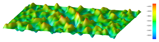
Figure 1: The random bottom topography sample # 1.

Here, we demonstrate how the MLMC method can be combined with an ocean circulation model to quantify the volume transport of the ACC. In order to stay focused on the methodology that is being explored here, we sharply reduce the physics of this problem while still retain its essential features. The fluid domain is a re-entrant rectangle that is $2,000$ km long and $1,733$ km wide; the same size as [3], and also see [27]. The flow is governed by a three-layer isopycnal model, which reads

$$\left\{\begin{aligned} &\dfrac{\partial h_{i}}{\partial t}+\nabla\cdot\left(h_{i}\mathbf{u}_{i}\right)=0,\\ &\dfrac{\partial\mathbf{u}_{i}}{\partial t}+h_{i}q_{i}\boldsymbol{\mathrm{k}}\times\mathbf{u}_{i}=-\nabla\left(\dfrac{\phi_{i}}{\rho_{0}}+K_{i}\right)+\mathbf{D}_{i}+\mathbf{F}_{i},\\ &\dfrac{\partial}{\partial t}(h_{i}\sigma_{i})+\nabla\cdot\left(h_{i}\sigma_{i}\mathbf{u}_{i}\right)=0,\\ \end{aligned}\right.$$ (66)

where $i=1,2,3$ is the layer index starting at the ocean surface. The prognostic variables $h_{i}$, $\mathbf{u}_{i}$ and $\sigma_{i}$ denote the layer thickness, horizontal velocity, and some tracer respectively, and the diagnostic variables $q_{i}$, $\phi_{i}$ and $K_{i}$ denote the potential vorticity, Montgomery potential and kinetic energy, respectively, and they are defined as

$$q_{i}=\dfrac{\nabla\times\mathbf{u}_{i}+f}{h_{i}},\qquad i=1,2,3,$$

$$K_{i}=\frac{1}{2}|\mathbf{u}_{i}|^{2},\qquad i=1,2,3,$$

$$\phi_{1}=p_{0}+\rho_{1}g(h_{1}+h_{2}+h_{3}+b),$$

$$\phi_{2}=\phi_{1}+(\rho_{2}-\rho_{1})g(h_{2}+h_{3}+b),$$

$$\phi_{3}=\phi_{2}+(\rho_{3}-\rho_{2})g(h_{3}+b),$$

with $p_{0}$ denoting the surface pressure and $b$ the bathymetry; $\mathbf{D}_{i}$ denotes the horizontal viscous diffusion, which usually takes the form of harmonic or biharmonic diffusion. The external forcing term $\mathbf{F}_{i}$ for each layer is specified as follows,

$$\mathbf{F}_{i}=\left\{\begin{aligned} &\dfrac{\boldsymbol{\tau}}{\rho_{1}h_{1}}\textrm{ (wind stress) },&&i=1,\\ &0,&&i=2,\\ &-\mathbf{d}\textrm{ (bottom drag) },&&i=3.\end{aligned}\right.$$ (67)

The model is made up of three isopycnal layers with mean layer thickness of 500 m, 1250 m and 3250 m and with densities of $1010\,\textrm{kg}\,\textrm{m}^{-3}$, $1013\,\textrm{kg}\,\textrm{m}^{-3}$ and $1016\,\textrm{kg}\,\textrm{m}^{-3}$. The system is forced by a zonal wind stress on the top layer with the form

$$\tau=\tau_{0}\sin^{2}\left(\dfrac{\pi y}{L_{y}}\right),$$

where $\tau_{0}=0.1\textrm{N}\,\textrm{m}^{-2}$. The uncertainty in the model is presented by the bottom topography. We assume that the bottom topography of the domain is largely flat with small but random features,

$$b=\sum_{k,l=4}^{20}\dfrac{H}{k^{2}+l^{2}}\left(a_{kl}(\omega)\cos\left(\dfrac{2\pi kx}{L_{x}}\right)+b_{kl}(\omega)\sin\left(\dfrac{2\pi kx}{L_{x}}\right)\right)\sin\left(\dfrac{l\pi y}{Ly}\right),$$

where $a_{kl}(\omega)$ and $b_{kl}(\omega)$ are random variables. Thus the bottom is controlled by 578 random parameters. One sample of the topography is shown in Figure 1. Similar types of bottom topography profiles have been used by [37]. The numerical simulations are conducted using the MPAS isopycnal ocean model ([35]). MPAS, which stands for Model Prediction Across Scales, implements a C-grid finite difference / finite volume scheme that is detailed in [36, 34]. MPAS utilizes arbitrarily unstructured Delaunay-Voronoi tessellations ([6, 7]). For this experiment, we have four levels of resolutions available: 10 km, 20 km, 40 km, and 80 km. To account for the effect of the unresolved eddies, the biharmonic hyperviscosity is used. The viscosity parameters are chosen to minimize the diffusive effect while still ensure a stable simulation. For the aforementioned resolutions, the viscosity parameters are $10^{9}\,\mathrm{m}^{4}\mathrm{s}^{-1}$, $10^{10}\,\mathrm{m}^{4}\mathrm{s}^{-1}$, $10^{11}\,\mathrm{m}^{4}\mathrm{s}^{-1}$, and $10^{12}\,\mathrm{m}^{4}\mathrm{s}^{-1}$, respectively. At the coarsest resolution (80 km), the Gent-McWilliams closure ([9, 10]) is turned on, with a constant parameter $400\,\mathrm{m}^{2}\mathrm{s}^{-1}$, to account for the cross-channel transport and to prevent the top fluid layer thickness from thinning to zero. GM is not used in any other higher resolution simulations. The configurations for each mesh resolution are summarized in Table 2. Each simulation is run for 40 years to spin up the current. The output data are saved every 10 days for the next 10 years.

	Eddy closures	Spatial DOFs	Time step (s)	Processes
10 km	Hyperviscosity	480,000	45	64
20 km	Hyperviscosity	120,000	90	16
40 km	Hyperviscosity	30,000	180	4
80 km	Hyper. + GM	7,500	360	1

Table 2: The configurations for each resolution. The spatial degrees of freedom (DOFs) is calculated as (number of cells + number of edges) $\times$ number of layers.

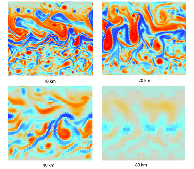
Figure 2: The snapshots of the vorticity field at year 40, computed with the random bottom topography sample #1.

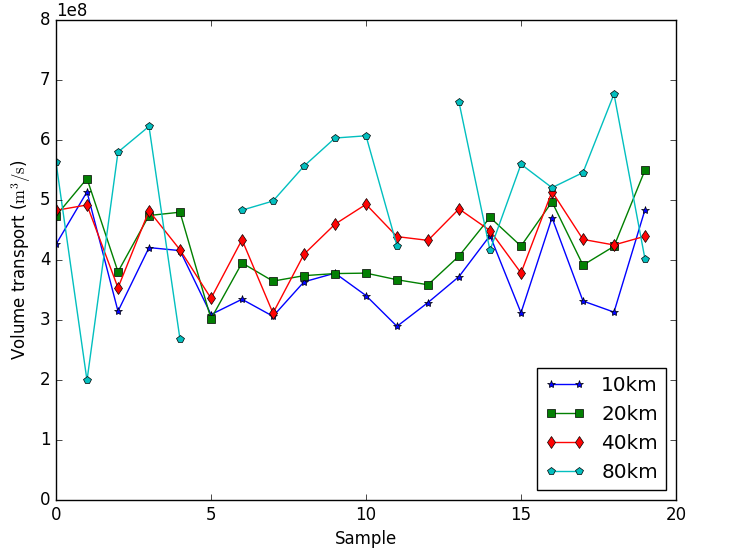
Figure 3: The changes of volume transport across a subset of the sample space.

The interior of large-scale geophysical flows has Reynolds numbers on the order of $10^{20}$. Thus the large-scale geophysical flows are turbulent in nature, and mesoscale and submesoscale eddy activities are important part of the ocean dynamics ([26, 5, 22, 15, 2]). For turbulent flows, the pointwise instantaneous behavior of the flow is not reliable anymore. But one can hope that observing the flow long enough can reveal reliable and useful statistics about the flow. Figure 2 shows the snapshots of the relative vorticity field on Year 40 for mesh resolutions with the same bottom topography profile. The highest resolution, 10km (Panel (a)), depicts a scene of rapid mixing by a wide range of mesoscale and submesoscale eddies. As the mesh gets coarser, the level of eddy activities decrease. The comparison also makes it clear that these flows are largely independent of each other, for there appears to be no correlation between the basic flow patterns of these simulations, other than the fact that they are all west-to-east flows driven by a common windstress. However, a comparison of the volume transport by these simulations over a common set of topographic profiles tells a different and reassuring story. In Figure (3), each curve represents results on one mesh resolution. While on any particular topography profile, the results from different resolutions do not agree, the curves across all the 20 samples, especially those for the 10 km, 20 km, and 40 km, largely follow the same pattern. The agreement of the patterns of the curves indicates that a great deal of information in the curve for the highest resolutions is actually available in the curves of the lower resolutions, and this is a vindication for the multi-level method that we are pursuing here.

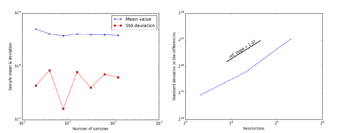
Figure 4: Sample mean and variance and the convergence rate. The mean and variance are estimated using samples from the 20km simulations.

In order to set up the MLMC simulations under the various strategies proposed before, three key parameters are needed: the standard deviation $\delta[U]$ in the true solution, the error $e$ in the finest solutions, and the convergence rate $\alpha$. To fully determine these key parameters requires the true solution itself $U$, which is not available in any practical applications. But they can easily estimated (see Section 2.3). Using data from the 20 km simulations, we compute the MC mean and the standard deviation according to the formulae (5) and (62). To probe the sensitivity of these estimates to the sample sizes, we compute the quantities with several independent sample sets with varying sizes, and the results are shown in Figure 4 (left panel). Based on this figure, we take

$$\delta[U]\approx 7.36\times 10^{7}\textrm{ m}^{3}/\textrm{s}.$$

Using the formula (64) and data from 10 km, 20 km, 40 km, and 80 km simulations (Figure 4 (right panel)), the convergence rate $\alpha$ is estimated to be

$$\alpha\approx 1.07.$$

This convergence appears slow but expected for long term simulations of turbulent flows. The underlying numerical scheme, namely a C-grid finite volume scheme, has been found to be accurate of orders $1\sim 2$ for laminar flows ([34], also see [4]). Finally the error $e$ in the finest solutions is calculated using the formula (65) and data from the 10km and 20km simulations,

$$e\approx 9.60\times 10^{6}\textrm{ m}^{3}/\textrm{s}.$$

	$L$	$m_{1}$	$m_{2}$	$m_{3}$	$m_{4}$	Comp. load
Classical MC	n/a	59				59
Strategy #1	3	11	48	210		22.4
Strategy #2	2	11	191			36.3
Strategy #3	3	876	763	210		1096.1
Strategy #4	2	11	763			107

Table 3: Multi-level setup under different strategies

Using these estimated parameters and the formulae set forth under various strategies propose in the previous section, we calculate the number of levels, the sample size at each level, and the computational load for each strategy for the multi-level method. The sample size and computational load for the classical Monte Carlo method are also calculated. The computational load are calculated in terms of the the computational load for one single simulation at the highest resolution (lowest level). The issue of efficiency, overhead, etc. are neglected. For example, the classical MC method requires 59 simulations at the highest resolution, and therefore its computational load is 59. The results are listed in Table 3. Several striking features are present in the results. First of all, under all strategies, the numbers of required levels are low (2 or 3). This can be attributed to the fact that the error in the finest solutions are high compare to the variance in the true solution. Second, the sample sizes at the lowest level (highest resolution) are identical for Strategy #1, 2 and 4 (11 for all three). This is no coincidence. A careful examination of the formulae (23), (32), (54) reveal that, at the lowest level $l=1$, the sample sizes for Strategies #1, 2, and 4 are identical, and depend on the convergence rate $\alpha$ only. Thus, irregardless of the actual highest resolution used, the sample sizes for this model at the lowest level will remain the same (=11) and identical for all three strategies. Finally, for Strategy #3, the sample size at the highest resolution is too high, and results in a computational load even higher than that of the classical Monte Carlo method. The reason is that this strategy requires a error distribution that is low at the highest resolution, and high at the lowest resolution. In terms of computational loads, Strategy #1 is the optimal choice, and it is followed by Strategy #2. Both strategies are better than the classical Monte Carlo method. Strategy #4 is actually more costly than the classical method, due to the bloated sample size at the next level.

	Est. volume	Est. error	CPU time	CPU efficiency
	transport ($\mathrm{m}^{3}/\mathrm{s}$)	($\mathrm{m}^{3}/\mathrm{s}$)	(hours)	(DOFs / CPU second)
Classical MC	$3.58\times 10^{8}$	$1.92\times 10^{7}$	158,446	343,172
Strategy #1	$3.55\times 10^{8}$	$4.80\times 10^{7}$	45,917	449,719
Strategy #2	$3.57\times 10^{8}$	$3.84\times 10^{7}$	68,457	488,013

Table 4: Comparison between the classical MC, and the MMC under strategies #1 and #2. The efficiency is calculated as Total DOFs / Total CPU time. Total DOFs is calculated as Spatial DOFs $\times$ Time steps $\times$ Number of samples.

We proceed to calculate the estimates and errors in the estimates using the classical MC method and the MLMC method under strategies #1 and 2. The results from the classical MC can serve as a reference, since by the analysis of 2.1, its error should be the smallest. Strategies #3 and 4 are not used due to the shear sizes of their computational loads. The classical MC and both Strategies #1 and 2 produce similar estimates, $\sim 3.58\times 10^{8}\textrm{ m}^{3}/\mathrm{s}$, for the volume transport (second column of Table 4). The error for each method is listed in the third column. The result of the classical MC method has an error of about 5.4%. The error for Strategy #1 is the largest, about 13.5%. This is expected, because the error for this strategy depends on the number of levels (see (28)), which is higher than that for Strategy #2.

The primary advantage of MLMC is efficiency. The first indicator for efficiency is of course the computational load that each method will incur, which has already be listed in Table 3. These numbers are the theoretical computational load, and takes no consideration of computational overhead, parallelization, etc. Here, we examine the actual efficiency for each method. First, we look at the total CPU hours used by each method (fourth column of Table 4). The MLMC with strategy #1 uses the least amount of CPU time, 45,917 CPU hours, a saving of $71\%$ compared with the MC method. Strategy #2 use 68,457 CPU hours, a saving of $67\%$.

The savings of MLMC strategies in the actual CPU times are largely in line with the savings in computational loads (Table 3), but appear more dramatic than what the latter would suggest. This is due to the increased CPU efficiency under the MLMC methods. It is well known that MC methods are easy to parallelize, and therefore highly scalable on supercomputers. The MLMC has the potential to increase the efficiency over the classical MC even further, by running more small-sized simulations and fewer large simulations. Due to the large sizes of the computations in this project, we are not able to perform a actual scalability analysis, which involves running the experiment with different numbers of total available processes. However, we can indirectly examine the issue of scalability by comparing the efficiency for each CPU core for the methods considered here (last column of Table 4). Compared with the classical MC, Strategy #1 increases the CPU efficiency by 31%, and Strategy #2 increases the CPU efficiency even more, by 42%.

4 Discussions

The success of the MLMC method relies on a crucial assumption, namely that, a lot of the information contained in high-resolution simulations is also available from low-resolution simulations, under the identical or similar model configurations. The higher the correlation, the better the MLMC method will work. For steady-state or laminar flows, especially when the simulations are backed up by rigorous error estimates, the correlation between high-resolution and low-resolution solutions is high and quantifiable, and the MLMC method works very well (see references cited in Introduction). For long-term simulations of turbulent flows, the situation is different. It is known that the pointwise behaviors of high- and low-resolution solutions of turbulent flows are uncorrelated (Figure 2). But pointwise behaviors of turbulent flows are of little interest. What are important are certain aggregated quantities such as mean SST. Then, naturally arise the questions as to whether these aggregated quantities are correlated across different resolutions, and whether the MLMC method can be used to save computation times. Through an experiment with the Antarctic Circumpolar Current, the present work gives affirmative answers to both of these questions. The conclusions drawn in this work cannot be generalized universally to all turbulent flows, because, after all, there is no universal theory for turbulent flows yet. But it is reasonable to expect that the same results should hold in similar situations. Specifically, the MLMC method can be effective in saving computation times when the QoI demonstrates a certain level of correlation across different resolutions.

Another objective of this paper is to explore how the MLMC simulation can be set up. Four different strategies are presented, based on the desired error distributions. One surprising finding is that the performance of each strategy, with regard to computational cost, depends on the convergence rate. For all strategies discussed, the higher the convergence rate is, the faster the computational cost will grow. This sounds counter-intuitive. Here, the focus is on how fast the total computational cost will grow in terms of the computational cost of a single high-resolution simulation (linearly, quadratically, etc.) Of course, for the same highest resolution, a higher convergence rate will eventually leads to more accurate results, and the associated higher computational cost is a price paid for this higher accuracy.

Among all the four strategies discussed in this work, Strategy #3, which amplify the sample sizes at high resolutions, seems to be of little use, because of the unreasonably high cost. Strategy #1 is the most natural choice, but it may lead to bigger margin of errors if the number of levels is high. In that situation, Strategy #2 & #4 can be used. In our experiment with the ACC, the highest resolution has 40,000 grid points, and Strategy #2 outperforms Strategy #4 with a lower computational cost. But it should be kept in mind that, even at a very modest convergence rate ($\alpha<1/2$), the computational cost for Strategy #2 grow polynomially with respect to the computational cost for a single high-resolution simulation. Therefore, it is conceivable that, as higher resolution are taken into use, Strategy #4 will eventually outperform Strategy #2.

References

- [1] Andrea Barth, Christoph Schwab, and Nathaniel Zollinger, Multi-level Monte Carlo Finite Element method for elliptic PDEs with stochastic coefficients, Numer. Math. 119 (2011), no. 1, 123–161.
- [2] Liam Brannigan, David P Marshall, Alberto Naveira-Garabato, and A J George Nurser, The seasonal cycle of submesoscale flows, Ocean Modelling 92 (2015), 69–84.
- [3] Qingshan Chen, T Ringler, and P R Gent, Extending a potential vorticity transport eddy closure to include a spatially-varying coefficient, Computers & Mathematics with Applications 71 (2016), no. 11, 2206–2217.
- [4] Qingshan Chen, Todd Ringler, and Max Gunzburger, A co-volume scheme for the rotating shallow water equations on conforming non-orthogonal grids, Journal of Computational Physics 240 (2013), 174–197.
- [5] G. Danabasoglu, JC MCWILLIAMS, and PR GENT, The Role of Mesoscale Tracer Transports in the Global Ocean Circulation, Science 264 (1994), no. 5162, 1123–1126.
- [6] Qiang Du, Vance Faber, and Max Gunzburger, Centroidal Voronoi tessellations: applications and algorithms, SIAM Review 41 (1999), no. 4, 637–676 (electronic).
- [7] Qiang Du, Max D. Gunzburger, and Lili Ju, Constrained centroidal Voronoi tessellations for surfaces, SIAM Journal on Scientific Computing 24 (2003), no. 5, 1488–1506 (electronic).
- [8] Peter R. Gent, William G Large, and Frank O Bryan, What sets the mean transport through Drake Passage?, Journal of Geophysical Research 106 (2001), no. C2, 2693.
- [9] Peter R. Gent and James C. McWilliams, Isopycnal Mixing in Ocean Circulation Models, Journal of Physical Oceanography 20 (1990), no. 1, 150–155.
- [10] Peter R. Gent, Jurgen Willebrand, Trevor J. McDougall, and James C. McWilliams, Parameterizing Eddy-Induced Tracer Transports in Ocean Circulation Models, Journal of Physical Oceanography 25 (1995), no. 4, 463–474.
- [11] Michael B Giles, Multilevel Monte Carlo Path Simulation, Operations Research 56 (2008), no. 3, 607–617.
- [12] , Multilevel Monte Carlo methods, Acta Numerica 24 (2015), 259–328.
- [13] J. M. Hammersley and D. C. Handscomb, Monte Carlo Methods, vol. 14, Applied Statistics, no. 2/3, Springer-Verlag, 1964.
- [14] Stefan Heinrich, Multilevel Monte Carlo Methods, Large-Scale Scientific Computing (Svetozar Margenov, Jerzy Waśniewski, and Plamen Yalamov, eds.), Springer Berlin Heidelberg, Berlin, Heidelberg, 2001, pp. 58–67.
- [15] William R Holland, The Role of Mesoscale Eddies in the General Circulation of the Ocean—Numerical Experiments Using a Wind-Driven Quasi-Geostrophic Model, http://dx.doi.org/10.1175/1520-0485(1978)008¡0363:TROMEI¿2.0.CO;2 8 (2010), no. 3, 363–392.
- [16] C W Hughes, M P Meredith, and K J Heywood, Wind-driven transport fluctuations through drake passage: A southern mode, J. Phys. Oceanogr 29 (1999), no. 8, 1971–1992.
- [17] F. Y. Kuo J. Dick and I. H. Sloan, High-dimensioanl integration: The quasi-Monte Carlo way, Acta Numerica 22 (2013), no. fasc. 2, 133–288.
- [18] Ahmed Kebaier, Statistical Romberg extrapolation: a new variance reduction method and applications to option pricing, Ann. Appl. Probab. 15 (2005), no. 4, 2681–2705.
- [19] F Kenney and E S Keeping, Mathematics Of Statistics-Part Two, D.Van Nostrand Company , Inc Princeton, ; New Jersey ; Toronto ; New York ; London, 1951.
- [20] Ralf Kornhuber, Christoph Schwab, and Maren-Wanda Wolf, Multilevel Monte Carlo finite element methods for stochastic elliptic variational inequalities, SIAM Journal on Numerical Analysis 52 (2014), no. 3, 1243–1268.
- [21] F. Y. Kuo and I. H. Sloan, Multi-level quasi-Monte Carlo finite element methods for a class of elliptic partial differential equations with random coefficients, Siam Journal on Numerical Analysis 50 (2012), no. 6, 3351–3374.
- [22] M Levy, P Klein, and A M Treguier, Impact of sub-mesoscale physics on production and subduction of phytoplankton in an oligotrophic regime, J Mar Res 59 (2001), no. 4, 535–565.
- [23] J Li, X Wang, and K Zhang, Multi-level Monte Carlo weak Galerkin method for elliptic equations with stochastic jump coefficients, Appl. Math. Comput. (2016).
- [24] J. S. Liu, Monte Carlo strategies in Scientific Computing, Springer-Verlag, 2001.
- [25] L. Martino M. F. Bugallo and J. Corander, Adaptive importance sampling in signal processing, Digital Signal Processing 47 (2015), 1–19.
- [26] James C McWilliams, Submesoscale, coherent vortices in the ocean, Rev. Geophys. 23 (1985), no. 2, 165–182.
- [27] James C. McWilliams and Julianna H S Chow, Equilibrium Geostrophic Turbulence .1. a Reference Solution in a Beta-Plane Channel, Journal of Physical Oceanography 11 (1981), no. 7, 921–949.
- [28] Nicholas Metropolis and S Ulam, The Monte Carlo Method, Journal of the American Statistical Association 44 (1949), no. 247, 335–341.
- [29] S Mishra and Ch Schwab, Sparse tensor multi-level Monte Carlo finite volume methods for hyperbolic conservation laws with random initial data, Math. Comp. 81 (2012), no. 280, 1979–2018.
- [30] S Mishra, Ch Schwab, and J Šukys, Multi-level Monte Carlo finite volume methods for nonlinear systems of conservation laws in multi-dimensions, Journal of Computational Physics 231 (2012), no. 8, 3365–3388.
- [31] , Multilevel Monte Carlo Finite Volume Methods for Shallow Water Equations with Uncertain Topography in Multi-dimensions, SIAM Journal on Scientific Computing 34 (2012), no. 6, B761–B784.
- [32] , Multi-level Monte Carlo finite volume methods for uncertainty quantification of acoustic wave propagation in random heterogeneous layered medium, Journal of Computational Physics 312 (2016), 192–217.
- [33] H. Niederreiter, Random number generation and quasi-monte carlo methods, vol. 88, Journal of the American Statistical Association, no. 89, Springer-Verlag, 1993.
- [34] T. D. Ringler, J Thuburn, J. B. Klemp, and W. C. Skamarock, A unified approach to energy conservation and potential vorticity dynamics for arbitrarily-structured C-grids, Journal of Computational Physics 229 (2010), no. 9, 3065–3090.
- [35] Todd Ringler, Mark Petersen, Robert L Higdon, Doug Jacobsen, Philip W. Jones, and Mathew Maltrud, A Multi-Resolution Approach to Global Ocean Modeling, Ocean Modelling 69 (2013), 211–232.
- [36] J Thuburn, TD Ringler, WC Skamarock, and JB Klemp, Numerical representation of geostrophic modes on arbitrarily structured C-grids, Journal of Computational Physics 228 (2009), no. 22, 8321–8335.
- [37] AM TREGUIER and JC MCWILLIAMS, Topographic Influences on Wind-Driven, Stratified Flow in a Beta-Plane Channel - an Idealized Model for the Antarctic Circumpolar Current, Journal of Physical Oceanography 20 (1990), no. 3, 321–343.
- [38] B A Warren, J H LaCasce, and P E Robbins, On the obscurantist physics of ”form drag” in theorizing about the circumpolar current, J. Phys. Oceanogr 26 (1996), no. 10, 2297–2301.
- [39] Pieter Wesseling, An introduction to multigrid methods, Pure and Applied Mathematics (New York), John Wiley & Sons, Ltd., Chichester, 1992.