A Semi-Analytic Approach To Valuing Auto-Callable Accrual Notes

Abstract

We develop a semi-analytic approach to the valuation of auto-callable structures with accrual features subject to barrier conditions. Our approach is based on recent studies of multi-assed binaries, present in the literature. We extend these studies to the case of time-dependent parameters. We compare numerically the semi-analytic approach and the day to day Monte Carlo approach and conclude that the semi-analytic approach is more advantageous for high precision valuation.

1 Introduction

Auto-callable structures are quite popular in the world of  structured products. On top of the auto-callable structure it is common to add features related to interest payments. Hence, combining range accrual instruments and auto-call options not only leads to interesting conditional dynamics, but gives an illustrative example of a typical structured product ref. [1]. In addition to the strong path dependence of the coupons the instrument’s final redemption becomes path dependent too. Intriguingly, within the Black–Scholes world one can obtain a closed form expression for the payoff of such a derivative. On the other side one can also rely on a straightforward Monte Carlo (MC) approach ref. [2]. Often the interest payment features embedded in the instrument accrue a fixed amount daily, related to some trigger levels of the underlyings. The standard approach for valuation of such instruments is a daily MC simulation. The goal of this paper is to propose an alternative semi-analytic approach (SA), which in some cases performs significantly better than the brute force day to day MC evaluation ref. [3]. As we are going to show, the complexity of the evaluation of the auto-call probabilities grows linearly with the number of observation times of the instrument and one may expect that at some point the MC approach would become more efficient. However, even in these higher dimensional cases the semi-analytic approach provides a better control of the sensitivities of the instrument, since contrary to the MC approach it does not rely on a numerical differentiation. A relevant question is what are the pros and cons of the above methods - i.e SA vs MC. We address this question performing a thorough numerical investigation.

Technically our work is heavily based on ref. [4], where a valuation formula for multi-asset, multi-period binaries is provided. In addition to applying theses studies to auto-callable and range accrual structures, we extend the main result of ref. [4] to the case of time-dependent parameters: volatilities, interest rates and dividend yields.

The paper is structured as follows: In section two we begin with a brief description of the type of derivative instrument that we are studying.

In section three we develop the quasi-analytic approach, extending the results of ref. [4] to the case of time dependent deterministic parameters obtaining an expression for the probability of an early redemption in terms of the multivariate cumulative normal distribution. Building on this approach we obtain similar expression for the payoff at maturity, subject to elaborate conditions. In addition we calculate the payoff of the coupons as a sum over multivariate barrier options ref. [5], using the developed SA approach to represent the pay-off of the latter in terms of multivariate cumulative normal distribution ref. [6].

Finally, in section four we apply our approach to concrete examples. We implement numerically both the SA and MC approaches and demonstrate the advantage of applying the SA approach to lower dimensional systems, especially when a high precision valuation is required.

2 The instrument

In this paper we analyse a type of instrument which combines the features of range accrual coupons with auto-call options.

–The instrument is linked to the performance of two correlated assets $S_{1}$ and $S_{2}$.

–The instrument has a finite number $M$ of observation times $T_{1},T_{2},\dots,T_{M}$. If at the observation time $T_{k}$ both assets $S_{i}$ are simultaneously above certain barriers $b_{i,\,k}$ the instrument redeems at 100%. This is the auto-call condition. To shift the valuation time at zero we define $\tau=T-t$ and discuss the observation times $\tau_{1}\,,\tau_{2}\,,\dots,\tau_{M}$.

–At the observation times the instrument pays coupons proportional to the number of days, in the period between the previous observation time and the present, in which both assets $S_{i}$ were above certain barriers $c_{i}$.

–If the instrument reaches maturity, it redeems at 100% if both assets $S_{i}$ are above certain percentage $\kappa$ of their spot prices at issue time $\bar{S}_{i}$. If at least one of the assets is bellow $\kappa\,\bar{S}_{i}$ the instrument pays only a part proportional to the minimum of the ratios $S_{i}/\bar{S}_{i}$.

3 Semi-analytic approach

In this section we outline our semi-analytic approach. We begin by providing a formula for the auto-call probability.

3.1 Indicator functions and common notations

Without loss of generality, it is assumed that the auto-callable structure has two underlyings. On the set of dates are imposed trigger conditions related to the auto-call feature. If the auto-call triggers have never been breached at the observation dates the auto-callable structure matures at its final maturity date. On the opposite case, if one of the auto-call triggers have been breached the instrument auto-calls at this particular date and has its maturity.

Let us denote with $P_{k}$ the probability to auto-call at observation time $\tau_{k}$. Note that this implies that at previous observation times the spot prices of the two assets where never simultaneously above the barriers $b_{i}$. We introduce the following notations: $X_{i,\,k}$ labels the spot value of the assets $S_{i}$ at observation time $\tau_{k}$.

Using the standard notations, if probability space $\left(\Omega,\digamma,\mathbf{P}\right)$ is given, and $A\in\digamma,$ than the indicator function is defined as $\mathbf{E}\left(\mathbf{1}_{A}\right)=P(A).$

Using the above definition, the auto-call probability at time $\tau_{k},$for the general case with $n$ underlying indices is then given by the expectation related to some probability measure $Q$ of the indicator function:

$$P_{k}=\mathbf{E}_{Q}\left(\mathbf{1}_{(X_{1,\,1}<\,b_{1,\,1})\cup(X_{2,\,1}<\,b_{2,\,1}),\,(X_{1,\,2}<\,b_{1,\,2})\cup(X_{2,\,2}<\,b_{2,\,2}),\,\dots,\,(X_{1,\,k}<\,b_{1,\,k})\cap(X_{2,\,k}<\,b_{2,\,k})}\right)\ .$$ (1)

In order to simplify the notation, hereafter we will omit the probability measure $Q.$ For the case of two underlyings, we can also define also the probability that the instrument will not auto-call after the first $k$ observation times:

$$\bar{P}_{k}=\mathbf{E}\left(\mathbf{1}_{(X_{1,\,1}<\,b_{1,\,1})\cup(X_{2,\,1}<\,b_{2,\,1}),\,(X_{1,\,2}<\,b_{1,\,2})\cup(X_{2,\,2}<\,b_{2,\,2}),\,\dots,\,(X_{1,\,k}<\,b_{1,\,k})\cup(X_{2,\,k}<\,b_{2,\,k})}\right)\ .$$ (2)

Note that at each observation time we have more than one possibilities reflected in the $\cup$ operation.

For example the event $(X_{1,\,1}<\,b_{1})\cup(X_{2,\,1}<\,b_{2})$ can be split into the three scenarios $(X_{1,\,1}<\,b_{1})\cap(X_{2,\,1}<\,b_{2})$, $(X_{1,\,1}<\,b_{1})\cap(X_{2,\,1}>\,b_{2})$, $(X_{1,\,1}>\,b_{1})\cap(X_{2,\,1}<\,b_{2})$.

We could do a bit better if we define $\tilde{X}_{1,\,s}=X_{1,\,s}/b_{1,\,s}$ and $\tilde{X}_{2,\,s}=X_{2,\,s}/b_{2,\,s}$. Then the condition $(X_{1,\,1}<\,b_{1,\,1})\cup(X_{2,\,1}<\,b_{2,\,1})$ can be split into the two conditions $(\tilde{X}_{1,\,1}<1)\cap(\tilde{X}_{1,\,1}\,{\tilde{X}_{2,\,1}}^{-1}<1)$, $(\tilde{X}_{2,\,1}\,{\tilde{X}_{1,\,1}}^{-1}<1)\cap(\tilde{X}_{2,\,1}<1)$. Therefore to evaluate $\bar{P}_{k}$ we need to sum over $2^{k}$ possible scenarios, each scenario containing $2k$ conditions. This requires summing over $2^{k}$ different $2k$-dimensional cumulative multivariate normal distributions [4], which is computationally overwhelming for large values of $k$. Fortunately, using de Morgan rules we can substantially reduce the computational cost.

Let us denote by ${\cal E}_{i}$ the event $(X_{1,\,i}<\,b_{1})\cup(X_{2,\,i}<\,b_{2})$, then the event $\bar{\cal E}_{i}$ is written as the single scenario $(X_{1,\,i}>\,b_{1})\cap(X_{2,\,i}>\,b_{2})$.

Using the well known probability relation

$$P\left(\bigcap\nolimits_{i=1}^{n}{\cal E}_{i}\right) = \sum\limits_{i}P\left({\cal E}_{i}\right)-\sum\limits_{i,j}P\left({\cal E}_{i}\cup{\cal E}_{j}\right)+\sum\limits_{i,j,k}P\left({\cal E}_{i}\cup{\cal E}_{j}\cup{\cal E}_{k}\right)+$$

$$...+\left(-1\right)^{n}P\left(\bigcup\nolimits_{i=1}^{n}{\cal E}_{i}\right)$$

and DeMorgan’s law

$$\overline{\left(\bigcup\nolimits_{i=1}^{n}{\cal E}_{i}\right)}=\bigcap\nolimits_{i=1}^{n}\overline{{\cal E}_{i}}$$

can be shown that

$$\bar{P}_{k}=P\left(\bigcap_{s=1}^{k}{\cal E}_{s}\right)=1+\sum_{s=1}^{k}\sum_{\sigma_{s}\in C_{s}^{k}}(-1)^{s}P\left(\bigcap_{j=1}^{s}\bar{{\cal E}}_{\sigma_{s}(j)}\right)\ .$$ (3)

where the second sum is over all (sorted in ascending order) combinations of $k$ elements $s-$th class, $C_{s}^{k}$. Note that there are again $2^{k}$ different terms, however only the last term is $2k$-dimensional.

In the same spirit we can obtain a formula for the auto-call probabilities $P_{k}$:

$$P_{k}=\sum_{s=0}^{k-1}\sum_{\sigma_{s}\in C_{s}^{k-1}}(-1)^{s}P\left(\bigcap_{j=1}^{s}\bar{{\cal E}}_{\sigma_{s}(j)}\cap\bar{{\cal E}}_{k}\right)\ ,$$ (4)

where we have used a convention: $\cap_{j=1}^{0}\bar{{\cal E}}_{\sigma_{0}(j)}\cap\bar{{\cal E}}_{k}=\bar{{\cal E}}_{k}$. Equations (3) and (4) can be rewritten in terms of indicator functions. For compactness it is convenient to adopt the notations of ref. [4]. We introduce a multi-index notation denoting by $X_{I}$ the element $X_{i,\,s}$, where $I=1\,,\dots\,,n$ and $n$ is the number of all observed assets’ prices. In the case considered in equation (1) we have $n=2\,k$. Using lexicographical order we can make the map explicit:

$$(i,s)\rightarrow I=I[i,\,s]=2\ast(s-1)+i\,$$ (5)

where we have used that $i=1,2$. Next we define the following notation:

$$(X^{A})_{j}={X}_{1}^{A_{j1}}\,\dots\,{X}_{n}^{A_{jn}}~{}~{}~{}~{}j=1\,,\dots\,,m\ ,$$ (6)

where $m$ is the number of barrier conditions and A is an $n\times m$ matrix. With these notations a general indicator function can be written as:

$$\mathbf{1}_{m}(S\,\mathbf{X}^{A}>S\,\mathbf{a})\,$$ (7)

where $\mathbf{a}$ is a vector of barriers and to allow for different types of inequalities we have introduced the $m\times m$ diagonal matrix $S$ whose diagonal elements take the values $\pm 1$ (’$+$’ for ’$>$’ and ’$-$’ for ’$<$’). Equations (3),(4) now become:

$$\bar{P}_{k}=\mathbf{E}\left(1+\sum_{s=1}^{k}\sum_{\sigma_{s}\in C_{s}^{k}}(-1)^{s}\mathbf{1}_{2s}(\mathbf{X}^{A(\sigma_{s})}>\mathbf{b}(\sigma_{s}))\right)\ ,$$ (8)

$$P_{k}=\mathbf{E}\left(\sum_{s=0}^{k-1}\sum_{\sigma_{s}\in C_{s}^{k-1}}(-1)^{s}\mathbf{1}_{2s+2}(\mathbf{X}^{\tilde{A}(\sigma_{s})}>\mathbf{\tilde{b}}(\sigma_{s}))\right)\ ,$$ (9)

where $\mathbf{A}(\sigma_{s})$, $\mathbf{b}(\sigma_{s})$, $\mathbf{\tilde{A}}(\sigma_{s})$, $\mathbf{\tilde{b}}(\sigma_{s})$, are $2k\times 2s$, $1\times 2s$, $2k\times 2(s+1)$, $1\times 2(s+1)$ matrices, respectively. Their non-zero entries are:

$$A(\sigma_{s})_{I[i,\,\sigma_{s}(j)],\,I[i,\,j]}=1,~{}~{}~{}(\mathbf{b}(\sigma_{s}))_{I[i,j]}=b_{i,\,\sigma_{s}(j)}\ ,$$ (10)

$$\tilde{A}(\sigma_{s})_{I[i,\,\sigma_{s}(j)],\,I[i,\,j]}=1,~{}~{}~{}(\mathbf{\tilde{b}}(\sigma_{s}))_{I[i,j]}=b_{i,\,\sigma_{s}(j)}\ ,$$ (11)

$$~{}~{}~{}\text{for}~{}~{}~{}i=1,2~{}\text{and}~{}j=1,\dots,s\ .$$

$$\tilde{A}(\sigma_{0})_{I[i,\,k],\,i}=1,~{}~{}~{}(\mathbf{\tilde{b}}(\sigma_{0}))_{i}=b_{i,\,k}\ ,~{}~{}~{}\text{for}~{}~{}i=1,2\ .$$ (12)

In equation (10) we have used the map (5). Note that it is crucial that the combinations $\sigma_{s}$ are sorted in ascending order.

3.2 A time-dependant valuation formula

If we restrict ourselves to time independent deterministic parameters (interest rate, dividend yield, volatility) we can directly apply the formula derived in ref. [4] to calculate the indicator functions in equations (8) and (9). However, this is a very crude approximation when dealing with long instruments this is why we extend the results of ref. [4] to the time dependent case. The starting point is to model the dynamics of the asset $S_{i}$ with a geometric Brownian motion:

$$\frac{dS_{i}}{S_{i}}=\left(r(s)-q_{i}(s)\right)ds+\sigma_{i}(s)\,dW_{i}(s)\ ,$$ (13)

where $W_{i}$ are correlated Brownian motions with correlation coefficient $\rho_{ij}$. Indeed the integrated form of equation (13) is:

$$S_{i}(\tau)=S_{i}^{(0)}\,\exp\left\{\int\limits_{0}^{\tau}\left(r(s)-q_{i}(s)-\frac{1}{2}\sigma_{i}(s)^{2}\right)ds+\int\limits_{0}^{\tau}\sigma_{i}\,dW_{i}(s)\right\}$$ (14)

For the asset $i$ at time $T_{k}$ we can write:

$$\log\tilde{X}_{i,k}=\log x_{i}+\left(\bar{r}_{i,k}-\bar{q}_{i,k}-\frac{1}{2}\,\bar{\sigma}_{i,k}^{2}\right)\tau_{k}+\bar{\sigma}_{i,k}\,\sqrt{\tau_{k}}\,Z_{i,k}\ ,$$ (15)

where $Z_{i,k}$ is given by:

$$Z_{i,k}=\frac{1}{\bar{\sigma}_{i,k}\sqrt{\tau_{k}}}\int\limits_{0}^{\tau_{k}}\,\sigma_{i}(s)\,dW_{i}(s)\$$ (16)

and

$$\bar{r}_{i,k} = \frac{1}{\tau_{k}}\int\limits_{0}^{\tau_{k}}ds\,r_{i}(s)\ ,$$

$$\bar{q}_{i,k} = \frac{1}{\tau_{k}}\int\limits_{0}^{\tau_{k}}ds\,q_{i}(s)\ ,$$ (17)

$${\bar{\sigma}}_{i,k}^{2} = \frac{1}{\tau_{k}}\int\limits_{0}^{\tau_{k}}ds\,\sigma_{i}(s)^{2}\ .$$

Following ref. [4] we define the quantities:

$$\mu = \left(\bar{r}_{i,k}-\bar{q}_{i,k}-\frac{1}{2}\,\bar{\sigma}_{i,k}^{2}\right)\tau_{k}\ ,$$

$$\Sigma = \text{diag\thinspace}(\bar{\sigma}_{i,k}\,\sqrt{\tau_{k}})\ .$$ (18)

which are straightforward generalisations of the corresponding definitions in the time independent case [4]. A bit more involved is the expression for the correlation matrix $R$ defined as:

$$R_{(i,k)(j,l)}\equiv\langle Z_{i,k}\,,Z_{j,l}\rangle\ .$$ (19)

Using equation (16) and the formula:

$$\left\langle\int\limits_{0}^{\tau_{1}}\sigma_{i}(s)\,dW_{i}(s)\,,\,\int\limits_{0}^{\tau_{2}}\sigma_{j}(r)\,dW_{j}(r)\right\rangle=\rho_{ij}\int\limits_{0}^{\min(\tau_{1},\tau_{2})}\sigma_{i}(\tau)\,\sigma_{j}(\tau)\,d\tau\ ,$$ (20)

we obtain:

$$R_{(i,k)(j,l)}=\frac{\rho_{ij}}{\sqrt{\tau_{k}\tau_{l}}\,\bar{\sigma}_{i,k}\bar{\sigma}_{j,l}}\int\limits_{0}^{\min(\tau_{k},\tau_{l})}\sigma_{i}(\tau)\,\sigma_{j}(\tau)\,d\tau\ .$$ (21)

Next following ref. [4] we define:

$$\Gamma = \Sigma\,R\,\Sigma^{\prime}\ ,$$ (22)

$$D = \sqrt{\text{diag}\left(A\,\Gamma\,A^{\prime}\right)}\ ,$$

$$C = D^{-1}\left(A\,\Gamma\,A^{\prime}\right)D^{-1}\ ,$$

$$\mathbf{d} = D^{-1}\left[\log(\mathbf{x}^{A}/\mathbf{a})+A\,\mu\right]\ .$$

Here it is used that $x_{i,k}=x_{i}$ for all $k=1,\dots,M$. In therms of these quantities the indicator function is given by the same expression as in ref. [4], but the underlying variables are given in eq. (22) and due to the time-dependence thay are different from those given in the work ref. [4],

$$\mathbf{1}_{m}(S\,\tilde{\mathbf{X}}^{A(\omega)}>S\,\mathbf{a})=\mathcal{N}_{m}(S\,\mathbf{d(\omega)},\,S\,C(\omega)\,S)\,\ ,$$ (23)

where $\mathcal{N}_{m}$ is the cumulative multivariate normal distribution (centred around zero).

Note that equations (3.2)–(23) are valid for any $n\times m$ matrix $A$ and any positive barrier vector $\mathbf{a}$.

3.3 Auto-call probability and final payoff

Applying equation (23) to calculate the auto-call probability $P_{k}$ we obtain:

$$P_{k}=\sum_{s=0}^{k-1}\sum_{\sigma_{s}\in C^{k-1}_{s}}(-1)^{s}\mathcal{N}_{2s+2}(\mathbf{d}(\sigma_{s})\,,C(\sigma_{s}))\ ,~{}~{}~{}k=1\,\dots M-1\ ,$$ (24)

where $\mathbf{d}(\sigma_{s})$ and $C(\sigma_{s})$ are obtained by substituting $\tilde{A}(\sigma_{s})$ and $\mathbf{b(\sigma_{s})}$ from equation (10) into equation (22). Note that the index $k$ in equation (24) runs from one to $M-1$. The reason is that the last observation time is the maturity.

Let us denote by $P_{\mathrm{mat}}$ the probability to reach maturity. Clearly we have:

$$P_{\mathrm{mat}}=1-\sum_{k=1}^{M-1}P_{k}\ ,$$ (25)

The probability $P_{\mathrm{mat}}$ can be split into two contributions:

$$P_{\mathrm{mat}}=P_{\mathrm{up}}+P_{\mathrm{down}}\,$$ (26)

Where $P_{\mathrm{up}}$ is the probability to reach maturity with both assets simultaneously above the barrier $\kappa\,\bar{S}_{i}$, and $P_{\mathrm{down}}$ is the probability at least one fo the assets to be bellow the barrier. In fact the probability $P_{\mathrm{up}}$ is exactly $P_{M}$, hence we can write:

$$P_{\mathrm{up}}=\sum_{s=0}^{M-1}\sum_{\sigma_{s}\in C^{k-1}_{s}}(-1)^{s}\mathcal{N}_{2s+2}(\mathbf{d}(\sigma_{s})\,,C(\sigma_{s}))\ .$$ (27)

Clearly this also determines $P_{\mathrm{down}}$ as $P_{\mathrm{down}}=P_{\mathrm{mat}}-P_{\mathrm{up}}$. To calculate the payoff at maturity we also need the average performance of the assets subject to the condition that the worst performing asset is bellow the barrier $\kappa\,\bar{S_{i}}$. The probability for this to happen is exactly $P_{\mathrm{down}}$, which is a function of the parameter $\kappa$.

Let us denote $\hat{X}_{i}=S_{i}/\bar{S}_{i}$ and define $\hat{X}=\mathrm{min}(\hat{X}_{1},\hat{X}_{2})$, the probability $P_{\mathrm{down}}$ can be written as:

$$P_{\mathrm{down}}=P(\hat{X}<\kappa)\ .$$ (28)

The average performance of the assets provided that at least one of the assets is bellow the barrier $\kappa$ is then proportional to the conditional expectation value $\langle\hat{X}\rangle|_{\hat{X}<\kappa}$:

$$\left\langle\mathrm{min}\left(\frac{S_{1}}{\bar{S}_{1}},\,\frac{S_{2}}{\bar{S}_{2}}\right)\right\rangle\Big{|}_{\hat{X}<\kappa}=-\frac{1}{P_{\mathrm{down}}}\int\limits_{0}^{\kappa}d\kappa\,\kappa\,\frac{dP_{\mathrm{up}}}{d\kappa}\ ,$$ (29)

where we have used that $dP_{\mathrm{mat}}/d\kappa=0$. Therefore, the payoff at maturity is given by:

$$V_{\mathrm{maturty}}=P_{\mathrm{up}}+P_{\mathrm{down}}\left\langle\mathrm{min}\left(\frac{S_{1}}{\bar{S}_{1}},\,\frac{S_{2}}{\bar{S}_{2}}\right)\right\rangle\Big{|}_{\hat{X}<\kappa}=P_{\mathrm{up}}-\int\limits_{0}^{\kappa}d\kappa\,\kappa\,\frac{dP_{\mathrm{up}}}{d\kappa}\ ,$$ (30)

In the next subsection we calculate the contribution of the coupons.

3.4 Coupon contribution

To obtain the total payoff we have to evaluate the contribution of the coupons. This can be done by summing over a type of two-asset binary (cash-or-nothing) options, conditional on the survival of the instrument to the appropriate accrual period. Indeed the probability at time $\tau$ both assets to be above the barrier is given by the probability for such an option to pay. In the case of the first accrual period this reduced to the standard two-asset binary option [7]. To write down a closed form expression for this probability we need to add one more observation time $\tau_{a}$, which will iterate over the accrual dates. Clearly the simplest case is when $0\leq t_{a}\leq\tau_{1}$, that is the first accrual period. In this case we apply formula (23), for just one observation time $\tau_{a}$, with $A=S=\mathbf{1}_{2}$ and $\mathbf{a}=\mathbf{c}$. In more details the probability the coupons to pay at time $\tau_{a}<T_{1}$, $P_{01}(\tau_{a})$ is given by:

$$P_{01}(\tau_{a}) = \mathcal{N}_{2}(\mathbf{d}_{2}(\tau_{a}),C_{2})\ ,$$

$$d_{i} = \frac{\log(\bar{S}_{i}/c_{i})+(\bar{r}-\bar{q}_{i}(\tau_{a})-\bar{\sigma}_{i}(\tau_{a})^{2}/2)\,\tau_{a}}{{\bar{\sigma}_{i}}(\tau_{a})\sqrt{\tau_{a}}}\ ,~{}~{}~{}i=1,2\ ,$$ (31)

$$C_{2} = \left(\begin{array}[]{cc}1&\rho_{12}\\ \rho_{21}&1\end{array}\right)$$ (34)

where $\bar{r},\bar{q}_{i}(\tau_{a})$ and $\bar{\sigma_{i}}(\tau_{a})$ are given by equations (3.2) with $\tau_{k}=\tau_{a}$. The total number of days in which coupons have been payed in the period $0$ to $\tau_{1}$, $N_{1}$ is then given by:

$$N_{1}=\sum_{\tau_{a}\,=\,1}^{\tau_{\,1}}P_{01}(\tau_{a})\ .$$ (35)

In the same way we can obtain a formula for the number of coupon days in the second accrual period. The only difference is that now in addition to the condition both assets to be above the accrual barrier we also have the condition that the instrument did not auto-call at time $\tau_{1}$. In general the probability the coupons to pay at time $\tau_{a}$ in the $k$-th accrual period is the joint probability that the instrument did not auto-call at the first $k-1$ observation times and both assets are above the accrual barrier at time $\tau_{a}$. Denoting by ${\cal E}^{C}_{\tau_{a}}$ the event that the assets are above the accrual barrier at time $\tau_{a}$ and using the notations from section 3.1, one can show that:

$$P_{k-1,k}(\tau_{a})=\sum_{s=0}^{k-1}\sum_{\sigma_{s}\in C_{s}^{k-1}}(-1)^{s}P\left(\bigcap_{j=1}^{s}\bar{{\cal E}}_{\sigma_{s}(j)}\cap{\cal E}^{C}_{\tau_{a}}\right)\ ,$$ (36)

where again we have used the convention: $\cap_{j=1}^{0}\bar{{\cal E}}_{\sigma_{0}(j)}\cap{\cal E}^{C}_{\tau_{a}}={\cal E}^{C}_{\tau_{a}}$. Equation (36) can be rewritten in analogy to equation (9) as:

$$P_{k-1,k}(\tau_{a})=\mathbf{E}\left(\sum_{s=0}^{k-1}\sum_{\sigma_{s}\in C_{s}^{k-1}}(-1)^{s}\mathbf{1}_{2s+2}(\mathbf{\tilde{X}_{\sigma_{s}}}>\mathbf{bc_{\sigma_{s}}})\ \right),$$ (37)

where $\mathbf{\tilde{X}_{\sigma_{s}}}$ is the vector: $[X_{1,\sigma_{s}(1)},\,X_{2,\sigma_{s}(1)},\,\dots\,,X_{1,\sigma_{s}(s)},\,X_{2,\sigma_{s}(s)},\,S_{1}(\tau_{a}),\,S_{2}(\tau_{a})]$ and $\mathbf{bc_{\sigma_{s}}}$ is the vector: $[b_{1,\sigma_{s}(1)},\,b_{2,\sigma_{s}(1)},\,\dots\,,b_{1,\sigma_{s}(s)},\,b_{2,\sigma_{s}(s)},\,c_{1},\,c_{2}]$. Denoting by $\tilde{C}_{\sigma_{s}}(\tau_{a})$ the covariant matrix constructed using equations (3.2)-(22) with times $\tau_{\sigma_{s}(1)},\,\dots,\,\tau_{\sigma_{s}(s)},\,\tau_{a}$ and denoting by $\mathbf{\tilde{d}_{\sigma_{s}}}$ the corresponding quantity in equation (22) constructed using the barrier vector $\mathbf{bc_{\sigma_{s}}}$, we can write:

$$P_{k-1,k}(\tau_{a})=\sum_{s=0}^{k-1}\sum_{\sigma_{s}\in C_{s}^{k-1}}(-1)^{s}\mathcal{N}_{2s+2}(\mathbf{\tilde{d}_{\sigma_{s}}}\,,\tilde{C}_{\sigma_{s}}(\tau_{a}))\ .$$ (38)

For the number of coupon paying days in the $k$-th accrual period we obtain:

$$N_{k}=\sum_{\tau_{a}\,=\,\tau_{k-1}\,+\,1}^{\tau_{k}}\,P_{k-1,k}(\tau_{a})\ .$$ (39)

To calculate the contribution of the coupons to the total payoff we need to take into account the discount factors, since we have assumed that the coupons are payed at the observation times. Note that the probability the coupons to pay already include the probability to reach that accrual period. Therefore, the total coupon contribution is given by:

$$VC_{M}=\gamma\,\sum_{s=1}^{M}\,e^{-\bar{r}_{s}\,\tau_{s}}\,N_{s}\ ,$$ (40)

where $\gamma$ is the daily rate of the coupon.

3.5 Total payoff

Assuming for simplicity that the instrument redeems at 100 % in the event of an auto-call (which in reality is quite common), for the total payoff we obtain:

$$V_{\mathrm{tot}} = V_{\mathrm{maturity}}+\sum_{k=1}^{M-1}e^{-\bar{r}_{k}\,\tau_{k}}\,P_{k}+VC_{M}$$ (41)

where we have substituted $P_{\mathrm{mat}}$ from equation (26).

4 Applications

In this section we outline some of the applications of the formalism developed above. We begin with the simplest case of a pure accrual instrument.

4.1 Pure accrual instrument

The pure accrual instrument that we consider in this subsection has the following characteristics:

–It pays a daily coupon at rate $\gamma$ if at closing time both assets $S_{i}$ are above the accrual barriers $c_{i}$

–At maturity (time $\tau_{m}$), it redeems at 100% if both assets $S_{i}$ are above certain percentage $\kappa$ of their spot prices at issue time $\bar{S}_{i}$. If at least one of the assets is bellow $\kappa\,\bar{S}_{i}$ the instrument pays only a part proportional to the minimum of the ratios $S_{i}/\bar{S}_{i}$.

Clearly this is the general instrument that we considered with the auto-call option removed. In this simple case the semi-analytic approach of section 3 is particularly efficient. The coupons are calculated by the first period formulas in equations (3.4), (35) with $\tau_{a}=\tau_{m}$, while the payoff at maturity is calculated using equation (30), with $P_{\mathrm{up}}$ given by:

$$P_{\mathrm{up}}=\mathcal{N}_{2}(\mathbf{\tilde{d}}_{2}(\tau_{m}),C_{2})\ ,$$ (42)

where $C_{2}$ is given in equation (3.4) and $\mathbf{\tilde{d}}_{2}(\tau_{m})$ is given by:

$$d_{i}=\frac{\log(\bar{S}_{i}/c_{i})+(\bar{r}-\bar{q}_{i}(\tau_{m})-\bar{\sigma}_{i}(\tau_{m})^{2}/2)\,\tau_{m}}{{\bar{\sigma}_{i}}(\tau_{m})\sqrt{\tau_{m}}}\ ,~{}~{}~{}i=1,2\ ,$$ (43)

where $\bar{r},\bar{q}_{i}(\tau_{m})$ and $\bar{\sigma_{i}}(\tau_{m})$ are given by equations (3.2) with $\tau_{k}=\tau_{m}$.

4.2 Dual index range accrual autocallable instrument

In this section we compare the efficiency of our semi-analytic (SA) approach and that of a standard Monte Carlo (MC) approach. Since the dimensionality of the SA problem increases linearly with the number of the auto-call dates, we consider the case of one auto-call date and two range accrual periods. Therefore, our problem is four dimensional and we would still need to rely on numerical methods to estimate the cumulative distributions.

To simplify the analysis even further and facilitate the comparison, we simplify the pay-off at maturity. The instrument pays 100% if both underlyings perform above the final barrier $\kappa$ (as before), but if this condition is not satisfied, instead of redeeming a worse performance: $\mathrm{min}\left({S_{1}}/{\bar{S}_{1}},\,{S_{2}}/{\bar{S}_{2}}\right)$ fraction, the instrument redeems at $\kappa\times 100\,\%$. Equation (30) then simplifies to:

$$V_{\mathrm{maturty}}=P_{\mathrm{up}}+\kappa\,P_{\mathrm{down}}\ .$$ (44)

The description of the coupon payments remains the same as in section 3.4. The volatilities $\sigma_{i}$, dividend yields $q_{i}$ , interest rate $r$ and correlation correlation coefficient $\rho$ used in the numerical example are presented in table 1. In addition the final barrier was set at 60% ($\kappa=0.60$) and the daily accrual rate used was (15/365)% ($\gamma=0.15/365$). The length of each accrual period was one year so that: $\tau_{1}=1$ and $\tau_{2}=2$.

$\sigma_{i}$	$q_{i}$	$r$	$\rho$
0.25	0.005	0.01	0.78
0.20	0.007	0.01	0.78

Table 1: Volatilities $\sigma_{i}$, dividend yields $q_{i}$, interest rate $r$ and correlation $\rho$ used in the numerical example.

To compare the efficiency of the algorithms we compared the running times $T_{\epsilon}$ as functions of the absolute error $\epsilon$. The resulting plot is presented in figure 1.

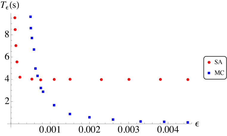
Figure 1: A plot of the running time $T_{\epsilon}$ in seconds as a function of the absolute error $\epsilon$. The round red dost represent the SA results, while the square blue dost correspond to the MC data.

The round dots correspond to the SA approach, while the square points represent the MC data. As one may expect, the running time $T_{\epsilon}$ for the MC algorithm increases as $\sim 1/\epsilon^{2}$ and while negligible for $\epsilon<0.01$, it increases rapidly to $\sim 10s$, for $\epsilon=5.0\times 10^{-4}$. On the other side the SA method has a steady computation time $T_{\epsilon}\sim 4s$, for $\epsilon<2.0\times 10^{-4}$. The SA and MC curves intersect at $\epsilon\approx 0.7\times 10^{-3}$. The advantage of using the SA method for higher precision $\epsilon<0.7\times 10^{-3}$ is evident. For example a calculation with $\epsilon=2.0\times 10^{-4}$ would require running the MC simulation for roughly $\sim 60\,s$, while the same accuracy can be achieved by the SA method for $\sim 5\,s$, which is a factor of twelve. Clearly the comparison depends on the implementation and the choice of parameters. To make the comparison fair we used MatLab for both methods. Using a vectorised MC algorithm for the Monte Carlo part and the built in MatLab cumulative distribution functions for the SA approach.

Another obvious advantage of the SA approach is the higher precision in the estimation of the sensitivities of the instrument. Semi-analytic expressions could be derided for most of the greeks, which enables their calculation with a limited numerical effort. This is clearly not the case in the MC approach, where one usually relies on a numerical differentiation.

Finally, as we pointed out at the beginning of this section the dimensionality of the problem increases linearly with the number of auto-call times. It is therefore expected that at some point the MC approach would become more efficient. Nevertheless, the SA approach could still be more efficient if the sensitivities are difficult to analyse in the MC approach.

5 Conclusion

This paper makes several contributions to the related literature.

Our main result is the development of a semi-analytical valuation method for auto-callable instruments embedded with range accrual structures. Our approach includes time-dependent parameters, and hence greatly facilitates practitioners. In the process we extend the valuation formula for multi-asset, multi-period binaries of ref. [4] to the case of time-dependent parameters, which the best of our knowledge is a novel result.

Another merit of this work is the comparison between the straightforward Monte Carlo and the semi-analytical approaches.Our comparison shows that the semi-analytical approach becomes more advantageous at higher precisions and is potentially order of magnitude faster than the brute force Monte Carlo method. The semi-analytical approach is also particularly useful when calculating the sensitivities of the instrument. It is widely accepted that the sensitivity calculations are often more important than the instrument price itself, due to their contribution for the correct instrument hedging.

Finally, our work can be used as a starting point for modelling more complex structures related to range accrual auto-callable instruments. Furthermore, although the numerical examples and the presented formulas are given for the two-dimension cases, multi-asset and multi-period generalisation of the formulas can be easily written using the key formulas presented here.

Acknowledgements:

We would like to thank Bojidar Ibrishimov for critically reading the manuscript.

Appendix A Proof of the valuation formula

For completeness we provide a proof of formula (23). Our proof follows the steps outlined in reference [4]. Using the definitions (6), (3.2) and equation (15) it is easy to obtain:

$$\log{\bf\tilde{X}}^{A}=\log{\bf x}^{A}+A\,{\bf\mu}+A\,\Sigma\,{\bf Z}\ .$$ (45)

Furthermore, the monotonicity of the logarithmic function implies:

$$\mathds{1}_{m}(S\,{\bf X}^{A}>S\,{\bf a})=\mathds{1}_{m}(S\,\log{\bf X}^{A}>S\,\log{\bf a})=\mathds{1}_{m}({\bf B\,Z}<{\bf b})\,\,$$ (46)

where:

$${\bf B} = -S\,A\,\Sigma\ ,$$ (47)

$${\bf b} = S\,(\log{\bf x}^{A}/{\bf a}+A\,{\bf\mu})\ .$$ (48)

Now we use a Lemma from ref. [4] (which we will prove for completeness):
Lemma 1. If B is an $\bf m\times n$ matrix of rank ${\bf m}\leq\bf n$ and ${\bf Z}$ is a random unit variate vector of length $\bf n$ with correlation matrix $\bf R$. Then:

$$E\left\{\mathds{1}_{m}(B{\bf\,Z}<{\bf b})\right\}={\cal N}_{m}(D^{-1}{\bf b},\,D^{-1}(B\,R\,B^{T})\,D^{-1})\,\ ,$$ (49)

where:

$$D=\sqrt{{\rm diag}(B\,R\,B^{T})}\ .$$ (50)

Applying Lemma 1 for ${\bf B}$ and $\bf b$ given in equation (47), we obtain:

$$D={\rm diag}(S\,A\,\Sigma\,R\,\Sigma^{T}\,A^{T}\,S)={\rm diag}(A\,\Sigma\,R\,\Sigma\,A^{T})={\rm diag}(A\,\Gamma\,A^{T})\ ,$$

$$D^{-1}\,(S\,A\,\Sigma\,)R\,(\Sigma\,A^{T}\,S)\,D^{-1}=S\,D^{-1}\,A\,\Sigma\,R\,\Sigma\,A^{T}\,D^{-1}\,S=S\,C\,S\ ,$$

$$D^{-1}\,{\bf b}=S\,D^{-1}\,(\log{\bf x}^{A}/{\bf a}+A.{\bf\mu})=S\,{\bf d}\ ,$$ (51)

where we have used that $S$ and $D$ are diagonal and commute and that $S_{i,i}^{2}=1$. Substituting relations (LABEL:relations) into equation (49) we arrive at equation (23). Now let us prove Lemma 1:
Proof: Let us complete the $m\times n$ matrix $B$ to an $n\times n$ non-singular matrix $\tilde{B}$. We write:

$$\tilde{B}=\begin{bmatrix}B\\ B_{\perp}\end{bmatrix}\ ,$$ (52)

where $B_{\perp}$ is an $(n-m)\times n$ matrix, which we are going to specify bellow. Consider the Cholesky decomposition of the correlation matrix $R$:

$$R=U\,U^{T}\ .$$ (53)

Next we transform the matrix $\tilde{B}$ with $U$ via $\tilde{B}^{\prime}=\tilde{B}\,U$, which implies:

$$B^{\prime} = B\,U\ ,$$ (54)

$$B_{\perp}^{\prime} = B_{\perp}\,U\ .$$ (55)

Since $B$ has rank $m$ and $U$ is invertible, $B^{\prime}$ also has a rank $m$. We can therefore think of $B^{\prime}$ as $m$ independent $n-column$ vectors. Spanning an $m$-dimensional subspace ${\cal L}^{m}$. We are always free to choose $B_{\perp}^{\prime}$ to be a matrix of $n-m$ independent $n-column$ vectors spanning the orthogonal completion of ${\cal L}^{m}$. Making this choice of $B_{\perp}^{\prime}$ implies:

$$B_{\perp}\,R\,B^{T}=B_{\perp}\,U\,(B\,U)^{T}=B_{\perp}^{\prime}{B^{\prime}}^{T}=0\ ,$$ (56)

Next we apply the transformation ${\bf Y}=\tilde{B}\,{\bf Z}$. The covariance matrix of the random vector $\bf Y$ is given by:

$$C=\tilde{B}\,R\,\tilde{B}^{T}=\begin{bmatrix}B\,R\,B^{T}&0\\ 0&B_{\perp}\,R\,B_{\perp}^{T}\end{bmatrix}\ ,$$ (57)

where we have used equation (56). Defining:

$${\bf Y_{||}}=B\,{\bf Z}\ ,~{}~{}~{}~{}{\bf Y_{\perp}}=B_{\perp}\,{\bf Z}\ ,$$ (58)

the condition $\mathds{1}_{m}(B{\bf\,Z}<{\bf b})$ becomes $\mathds{1}_{m}({\bf Y_{||}}<{\bf b})$. Furthermore, the probability density function of $\bf Y$ factorises:

$$\rho({\bf Y}) = \frac{1}{(2\pi)^{n/2}\sqrt{\det(\tilde{B}\,R\,\tilde{B}^{T})}}\exp\left(-\frac{1}{2}{\bf Y}^{T}\,(\tilde{B}\,R\tilde{B}^{T})^{-1}\,{\bf Y}\right)=$$ (59)

$$= \frac{1}{(2\pi)^{(n-m)/2}\sqrt{\det(B_{\perp}\,R\,B_{\perp}^{T})}}\exp\left(-\frac{1}{2}{\bf Y}_{\perp}^{T}\,(B_{\perp}\,R\,B_{\perp}^{T})^{-1}\,{\bf Y}_{\perp}\right)\times$$

$$\times \frac{1}{(2\pi)^{m/2}\sqrt{\det(B\,R\,B^{T})}}\exp\left(-\frac{1}{2}{\bf Y}_{||}^{T}\,(B\,R\,B^{T})^{-1}\,{\bf Y}_{||}\right)=$$

$$= \rho_{\perp}({\bf Y}_{\perp})\times\rho_{||}({\bf Y}_{||})$$

Since there are no conditions imposed on ${\bf Y}_{\perp}$ the integral over $\rho_{\perp}({\bf Y}_{\perp})$ is simply unity. What remains is the integral over $\rho_{||}({\bf Y}_{||})$, which upon the normalisation: ${\bf Y}_{\perp}\to D^{-1/2}{\bf Y}_{\perp}$ gives equation (49).

References

• [1] M. Bouzoubaa and A. Osseiran (2010). ”Exotic Options and Hybrids - A Guide to Structuring, Pricing and Trading”, 2010 John Wiley & Sons, Ltd,
• [2] P. Glasserman (2003). ”Monte Carlo Methods in Financial Engineering”, 2003 Springer ,
• [3] R. Korn, E. Korn and G. Kroisandt (2010). ”Monte Carlo Methods and Models in Finance and Insurance”, 2010 Taylor and Francis Group, LLC,
• [4] Max Skipper and Peter Buchen (2009). ”A valuation formula for multi-asset, multi-period binaries in a Black–Scholes economy”. The ANZIAM Journal, 50, pp 475-485. doi:10.1017/S1446181109000285,
• [5] J. Hull (2015). ”Options, Futures, and other Derivatives, 9ed.”, 2015, 2012, 2009 Pearson Education,
• [6] P. Zhang (1998). ”Exotic Options, 2ed.”, 1998 World Scientific,
• [7] R. C. Heynen and H. M. Kat (1996). ”Brick by Brick”, Risk Magazine, 9(6).