Nonequilibrium phase transitions in isotropic Ashkin-Teller Model

Ümit Akıncı

Department of Physics, Dokuz Eylül University, TR-35160 Izmir, Turkey

1 Abstract

Dynamic behavior of an isotropic Ashkin-Teller model in the presence of a periodically oscillating magnetic field has been analyzed by means of the mean field approximation. The dynamic equation of motion has been constructed with the help of a Glauber type stochastic process and solved for a square lattice.

After defining the possible dynamical phases of the system, phase diagrams have been given and the behavior of the hysteresis loops has been investigated in detail. The hysteresis loop for specific order parameter of isotropic Ashkin-Teller model has been defined and characteristics of this loop in different dynamical phases have been given.

Keywords: Dynamic isotropic Ashkin-Teller model; hysteresis loops; hysteresis loop area

2 Introduction

Ashkin-Teller Model (ATM) has been introduced for description of the cooperative phenomena of quaternary alloys [1]. It has four states per site and may be useful to describe magnetic systems with two easy axes. The ATM is a ‘staggered’ version of the eight-vertex model [2]. In two dimension, the ATM can be mapped onto a staggered eight-vertex model at the critical point. The non-universal critical behavior along a self-dual line, where the exponents vary continuously [3], is one of the interesting critical property of the model. On the other hand it has been shown that, three dimensional model has much richer phase diagrams than the ATM in two dimension [4]. There appear some first-order phase transitions and continuous phase transitions, even an XY -like transition and a Heisenberg-like multicritical point.

It has been shown that ATM could be described in Hamiltonian form appropriate for spin systems [5]. In this form, the model can be viewed as two coupled Ising models which is named as 2-color ATM. If two of these Ising models are identical then the model named as isotropic Ashkin-Teller model (IATM), otherwise the model is anisotropic Ashkin-Teller model (AATM). In a similar manner, ATM that formed by $N$ coupled Isig model entitled as N-color ATM as introduced in [6].

One of the well known physical realizations for this model is the compound of Selenium adsorbed on a Ni surface [7]. ATM can be used to describe chemical interactions in metallic alloys [8], thermodynamic properties in superconducting cuprates (ATM represents the interactions between orbital current loops in $CuO_{2}$ -plaquettes) [9] and elastic response of DNA molecule to external force and torque [10]. Besides, oxygen ordering in $YBa_{2}Cu_{3}O_{z}$ may also be understood in analogy with the two-dimensional IATM [11, 12, 13]. Also, ATM has many interesting applications in neural networks [14] and cosmology [15]. Besides, some mappings between the ATM and some other models are possible. This makes the ATM valuable in a theoretical manner. For instance, the random N-color quantum ATM can be described by an $O(N)$ Gross-Neveu model with random mass [16]. Similarly the relation between the two-dimensional N-component Landau-Ginzburg Hamiltonian with cubic anisotropy and N-color ATM has been discussed in [17, 18].

Critical properties of the ATM has been widely investigated in literature. IATM has been investigated by mean field renormalization group technique [19, 20], Monte Carlo Simulation (MC) [21, 22, 23, 24, 25, 26, 27], effective field theory (EFT) [28], transfer-matrix finite-size-scaling method [29], high and low temperature series expansion and MC [30], MC and renormalization group technique [31, 32] and damage spreading simulation [33, 34, 35].

On the other hand, the AATM has been investigated within several techniques such as, mean field approximation (MFA) [36], MC [37, 38], real-space renormalization-group approach [39] and Monte Carlo renormalization group technique [40].

Theoretical works devoted to ATM is not limited to regular (translationally invariant lattices) lattices. For instance, the model has been solved on Bethe Lattice [41], diamond-like hierarchical lattice [42, 43] and Cayley tree [44].

Also, some extensions and variants of the model have been studied. Extended ATM (ATM with reduced degeneracy) has been introduced [45] and solved within the MFA [46], mean field renormalization group technique [47] and MC [48]. Some other extensions like ATM with Dzyaloshinskii –Moriya interaction [49], ATM with spin-1 [50, 51], as well as mixed spin ATM [52] can be found in the literature.

Likewise, N-color ATM introduced in [6] has been investigated within the transfer matrix analysis [53], renormalization group technique [54], Monte Carlo renormalization group technique [55], MFA and MC [56]. This model has also been solved exactly for large N in 2D [57, 58].

Although, magnetic systems under a time dependent external magnetic field has been attracted much interest from both theoretical and experimental points of view; to the best of our knowledge, ATM under the time dependent magnetic field has not yet been studied. It will be interesting to investigate the dynamic character of ATM, which has rich critical properties in the static case, and obtain the corresponding dynamic phases of the system.

Dynamic phase transition (DPT) in magnetic systems comes from the competition between the relaxation time of the system and period of the driving periodic external magnetic field [59]. The time average of the magnetization over a full period of the oscillating magnetic field can be used as dynamic order parameter (DOP) of the system. On the other hand appeared hysteresis behavior from the delay of the response of the system to the driving cyclic force includes important clues of the dynamic character of the system.

From the experimental point of view, DPTs and hysteresis behaviors can be observed experimentally in different types of magnetic systems. Experiments on ultrathin Co films [60], Fe/Au(001) films [61], epitaxial Fe/GaAs(001) thin films [62], fcc Co(001), and fcc NiFe/Cu/Co(001) layers [63] Fe/InAs(001) ultrathin films [64] are among them.

On the theoretical side, there has been growing interest in the DPT which was first observed within the MFA [65] for the s-$1/2$ Ising model. Since that time, DPT and hysteresis behaviors of the s-$1/2$ Ising model have been widely studied within the several techniques such as MFA [66], Monte Carlo simulation (MC) [67], effective field theory (EFT) [68].

The aim of this work is to investigate the IATM under a magnetic field oscillating in time within the MFA formulation and Glauber type of stochastic process [69]. For this aim the paper is organized as follows: In Sec. 3 we briefly present the model and formulation. The results and discussions are presented in Sec. 4, and finally Sec. 5 contains our conclusions.

3 Model and Formulation

The Hamiltonian of the dynamical IATM is given by

$$\mathcal{H}=-J_{2}{{\underset{<i,j>}{\overset{}{\displaystyle\sum}}}\left(\sigma_{i}\sigma_{j}+s_{i}s_{j}\right)}-J_{4}{{\underset{<i,j>}{\overset{}{\displaystyle\sum}}}\sigma_{i}\sigma_{j}s_{i}s_{j}}-H(t){{\underset{i}{\overset{}{\displaystyle\sum}}}\left(\sigma_{i}+s_{i}\right)},$$ (1)

where the first two summations are over the nearest neighbors of the lattice, while the last one is over all the lattice sites. Here, $\sigma_{i}$ and $s_{i}$ are the $z$ components of the spin variables at a site $i$, $J_{2}$ is the bilinear exchange interactions of both of the Ising models. $J_{4}$ is the four spin interaction, which couples two Ising models to produce the IATM. Dynamical character of the model comes from the time dependent external longitudinal magnetic field $H(t)$ and it is given by

$$H(t)=H_{0}\sin{\left(\omega t\right)},$$ (2)

where $H_{0}$ is the amplitude and $\omega$ is the angular frequency of the periodic magnetic field and $t$ stands for the time.

In the static case (i.e. $H_{0}=0$) the model turns to the IATM, which is equivalent to the four component Potts model for $J_{2}=J_{4}$ [70]. When $J_{4}=0$ the model reduces to two independent Ising models.

We use a Glauber-type stochastic process [69] to investigate dynamic properties of the considered system. In general, in the Glauber type of stochastic process (as done in Ref. [65] for the Ising model) the thermal average (denoted with $\left\langle\right\rangle$) of a spin variable $\tau_{i}$, which can take values $\pm 1$ can be given as

$$\theta\frac{d\left\langle\tau_{i}\right\rangle}{dt}=-\left\langle\tau_{i}\right\rangle+\left\langle\frac{Tr_{i}\tau_{i}\exp{\left(-\beta\mathcal{H}_{i}\right)}}{Tr_{i}\exp{\left(-\beta\mathcal{H}_{i}\right)}}\right\rangle$$ (3)

in this type of process. Here, $\theta$ is the transition rate per unit time, $\beta=1/(k_{B}T)$, $k_{B}$ and $T$ denote the Boltzmann constant and temperature, respectively. $Tr_{i}$ stands for the trace operation over the site $i$. Also $\mathcal{H}_{i}$ denotes the part of the Hamiltonian of the system related to the site $i$, which is given by,

$$\mathcal{H}_{i}=-J_{2}\sigma_{i}{{\underset{j}{\overset{}{\displaystyle\sum}}}\sigma_{j}}-J_{2}s_{i}{{\underset{j}{\overset{}{\displaystyle\sum}}}s_{j}}-J_{4}\sigma_{i}s_{i}{{\underset{j}{\overset{}{\displaystyle\sum}}}\sigma_{j}s_{j}}-H(t)\left(\sigma_{i}+s_{i}\right),$$ (4)

where all summations are carried over the nearest neighbor sites of the site $i$.

In order to handle these spin-spin interactions, usual approximation can be adopted, that is; all spin-spin interactions of these variables are represented by local fields as

$$h_{1}=J_{2}{{\underset{j=1}{\overset{z}{\displaystyle\sum}}}\sigma_{j}},\quad h_{2}=J_{2}{{\underset{j=1}{\overset{z}{\displaystyle\sum}}}s_{j}},\quad h_{4}=J_{4}{{\underset{j=1}{\overset{z}{\displaystyle\sum}}}\sigma_{j}s_{j}},$$ (5)

where $z$ is the coordination number (i.e. number of nearest neighbor sites of any site $i$) of the lattice. Then one spin cluster Hamiltoian gets the form

$$\mathcal{H}_{i}=-\sigma_{i}h_{1}-s_{i}h_{2}-\sigma_{i}s_{i}h_{4}-\left(\sigma_{i}+s_{i}\right)H(t)$$ (6)

By writing Eq. (6) in Eq. (3) and performing the $Tr_{i}$ operations we can get equations for $\tau_{i}=\sigma_{i},s_{i}$ and $\sigma_{i}s_{i}$ as

$$\theta\frac{d\left\langle\sigma_{i}\right\rangle}{dt}=-\left\langle\sigma_{i}\right\rangle+\left\langle F\left(x,y,z\right)|_{x=h_{1}+H(t),y=h_{2}+H(t),z=h_{4}}\right\rangle$$

$$\theta\frac{d\left\langle s_{i}\right\rangle}{dt}=-\left\langle s_{i}\right\rangle+\left\langle F\left(x,y,z\right)|_{x=h_{2}+H(t),y=h_{1}+H(t),z=h_{4}}\right\rangle$$ (7)

$$\theta\frac{d\left\langle\sigma_{i}s_{i}\right\rangle}{dt}=-\left\langle\sigma_{i}s_{i}\right\rangle+\left\langle F\left(x,y,z\right)|_{x=h_{4},y=h_{1}+H(t),z=h_{2}+H(t)}\right\rangle$$

where

$$F\left(x,y,z\right)=\frac{\tanh{(\beta x)}+\tanh{(\beta y)}\tanh{(\beta z)}}{1+\tanh{(\beta x)}\tanh{(\beta y)}\tanh{(\beta z)}}$$ (8)

The simplest way to one calculate Eq. (7) is adopt MFA. Within this approximation, all local fields defined in Eq. (5) written in terms of the thermal averages of the spin variables,

$$h_{1}=zJ_{2}m_{\sigma},\quad h_{2}=zJ_{2}m_{s},\quad h_{4}=zJ_{4}m_{\sigma s},$$ (9)

where

$$m_{\sigma}=\left\langle\sigma_{j}\right\rangle,m_{s}=\left\langle s_{j}\right\rangle,m_{\sigma s}=\left\langle\sigma_{j}s_{j}\right\rangle.$$ (10)

Here, the translationally invariance property of the lattice is adopted, i.e. all lattice sites are equivalent. Then Eq. (7) gets the form

$$\theta\frac{dm_{\sigma}}{dt}=-m_{\sigma}+F\left(x,y,z\right)|_{x=h_{1}+H(t),y=h_{2}+H(t),z=h_{4}}$$

$$\theta\frac{dm_{s}}{dt}=-m_{s}+F\left(x,y,z\right)|_{x=h_{2}+H(t),y=h_{1}+H(t),z=h_{4}}$$ (11)

$$\theta\frac{dm_{\sigma s}}{dt}=-m_{\sigma s}+F\left(x,y,z\right)|_{x=h_{4},y=h_{1}+H(t),z=h_{2}+H(t)}$$

We can obtain explicit form of the dynamic equation of motion Eq. (11), by writing local fields defined in Eq. (9) into the function Eq. (8) given with order in Eq. (11). Eq. (11) is a coupled first order differential equation system and can be solved with standart methods such as Runge-Kutta method [71]. This iterative method starts by some initial values of the order parameters ($m_{\nu}(0)$, $\nu=\sigma,s,\sigma s$) and results in the desired solution after the convergency criteria $m_{\nu}\left(t\right)=m_{\nu}\left(t+2\pi/\omega\right)$ is satisfied. By this way we can obtain DOP as

$$Q_{\nu}=\frac{\omega}{2\pi}{{\underset{}{\overset{}{\displaystyle\oint}}}m_{\nu}\left(t\right)dt}$$ (12)

where $m_{\nu}\left(t\right)$ is a stable and periodic function. Dynamical critical points can be determined by obtaining the variation of the $Q_{\nu}$ with temperature for given set of Hamiltonian parameters.

We can construct the hysteresis loops which are nothing but the variation of the $m_{\nu}(t)$ with $H(t)$ in one period of the periodic magnetic field. Hereafter, once the hysteresis loop is determined, some quantities about it can be calculated. One of them is dynamical hysteresis loop area (HLA) and can be calculated via integration over a complete cycle of the magnetic field,

$$A_{\nu}={{\underset{}{\overset{}{\displaystyle\oint}}}}m_{\nu}\left(t\right)dH$$ (13)

and corresponds to the energy loss due to the hysteresis.

4 Results and Discussion

In order to determine DPT and hysteresis characteristics of the system, let us scale all Hamiltonian parameters with $J_{2}$, i.e. the unit of energy is $J_{2}$,

$$K_{4}=\frac{J_{4}}{J_{2}},\tau=\frac{k_{B}T}{J_{2}},h_{0}=\frac{H_{0}}{J_{2}},h(t)=\frac{H(t)}{J_{2}}.$$ (14)

Our investigation will be restricted to square ($z=4$) lattice. We set $\theta=1$ throughout our numerical calculations. We note that, under the transformation $\sigma_{i}\rightarrow s_{i}$, Hamiltonian and the formulation used here do not change, then it will be enough to investigate only one of the $m_{\sigma}$ or $m_{s}$, due to the fact that $m_{\sigma}=m_{s}$.

Different phases of the static model is well known:

• Ferromagnetic (Baxter) phase: All magnetizations are different from zero.

• Paramagnetic phase: All magnetizations are zero.

• $\left\langle\sigma s\right\rangle,\left\langle\sigma\right\rangle,\left\langle s\right\rangle$ phases : All magnetizations are zero except the magnetization that have index which is the name of the phase. For instance in $\left\langle\sigma\right\rangle$ phase only $m_{\sigma}$ is different from zero, while other two are equal to zero.

We investigate corresponding dynamical phases in this work. Three different dynamical phases (corresponding to the phases of the static IATM) will manifest themselves. Also, as discussed in Ref. [65] and successive works related to the DPT in Ising model, some regions may appear in the phase diagram, which is overlap region of the dynamically ordered and disordered phases. This overlap region mostly occur for relatively large values of $h_{0}$ for the Ising model. Let us enumerate these phases with prefix DP (which stands for dynamical phase).

• DP1: All DOPs are different from zero (corresponds to the Baxter phase in static the case )

• DP2: All DOPs are equal to zero (corresponds to the paramagnetic phase in static the case )

• DP3: Only $m_{\sigma s}$ is different from zero while $m_{\sigma}=m_{s}=0$ (corresponds to the $\left\langle\sigma s\right\rangle$ phase in static the case )

• DP4: Overlap of the DP1 and DP2 (or DP3) phases.

These phases and borders between them can be determined by calculating magnetizations defined in Eq. (10) by using formulation presented in this work. Typical time series corresponding to these four different phases can be seen in Fig. 1.

Figure 1: Time series of the order parameters of the IATM which corresponding to (a) DP1, (b) DP4, (c) DP3 and (d) DP2. All time series are calculated for the Hamiltonian parameters $K_{4}=0.5,\omega=1.0,h_{0}=0.5$. Initial values of the order parameters and temperature are shown in each figure. In each figure, the thicker lines correspond to $m_{\sigma}=m_{s}$ and the thinner lines correspond to $m_{\sigma s}$. $\nu$ stands for $\sigma,s,\sigma s$.

Although the values of the magnetizations in the DP1, DP2 and DP3 phases are not dependent on the initial values of the magnetizations, as one can see from to Fig. 1 (b) that, this does not hold for the DP4 phase. The value of the $m_{\sigma}=m_{s}$ converges zero or specific nonzero values depending on the initial value. In other words, formulation gives two different values (such that one of them is zero) for $m_{\sigma}=m_{s}$ depending on the choice of the initial values.

The phase diagram for static IATM in $(K_{4},\tau)$ plane can be seen in Fig. (2). This diagram can be obtained by numerical solutions of the Eq. (11) in the static limit. The same phase diagram obtained within the RG [19, 20] and MC [25] can be found in the literature. In the static IATM, for the higher values of the $K_{4}$, $\left\langle\sigma s\right\rangle$ phase may appear when the temperature rises, as seen in Fig. 2.

Figure 2: Phase diagram of the static IATM in the $(K_{4},\tau)$ plane.

4.1 Dynamic Phase Boundaries

Dynamic Phase Boundaries (DPB) of the model separate the different dynamic phases of the model. The relation of the dynamic behavior of the system with driving dynamical magnetic field is well known [59]. The relation between the exchange interaction, temperature, amplitude and the frequency of the magnetic field determines the dynamic phase of the system. Ferromagnetic exchange interaction of the model tends to to keep the nearest neighbors of the spins of the system parallel to each other. Rising temperature gives rise to the thermal thermal fluctuations and drive the system to the disordered phases. Besides, in the dynamical case, the amplitude and the frequency of the magnetic field are also decisive. Higher amplitude, dictates the spins to align parallel to the field. But when the frequency is high, spins cannot follow to magnetic field due to the difference between the period of the magnetic field and relaxation time of the spins.

In order to compare with the static case, let us depict the phase diagrams in $(K_{4},\tau)$ plane (as in Fig. 2) for some selected values of $\omega$ and $h_{0}$. This can be seen in Fig. 3 for low frequency ($\omega=0.1$) and in Fig. 4 for high frequency ($\omega=5.0$), with selected values of $h_{0}=0.1,0.2,0.5,1.0$ shown in figures labeled as (a),(b),(c) and (d) respectively.

Figure 3: Phase diagrams of the dynamical IATM in a $(K_{4},\tau)$ plane for selected values of $\omega=0.1$ and (a) $h_{0}=0.1$, (b) $h_{0}=0.2$, (c) $h_{0}=0.5$, (d) $h_{0}=1.0$.

Figure 4: Phase diagrams of the dynamical IATM in a $(K_{4},\tau)$ plane for selected values of $\omega=5.0$ and (a) $h_{0}=0.1$, (b) $h_{0}=0.2$, (c) $h_{0}=0.5$, (d) $h_{0}=1.0$.

As seen in Fig. 3, at low frequencies, rising amplitude shrinks the $DP_{1}$ region and shifts the $DP_{2}$ region towards the higher temperature region of the $(K_{4},\tau)$ plane. Also disappearing of the $DP_{4}$ phase with rising $h_{0}$ draws attention. The same reasoning holds for the high frequency regime, which can be seen in Fig. 4. For higher frequency the $DP_{4}$ phase survives in a larger interval of $h_{0}$, e.g. while for the value of $h_{0}=1.0$, high frequency has $DP_{4}$ phase in $(K_{4},\tau)$ plane (Fig. 4 (d)), the same phase don’t occur for lower frequency (Fig. 3 (d)). This behavior is similar to the behavior of the dynamical Ising model as shown in [65].

4.2 Hysteresis characteristics

The hysteric response of the system to the varying temperature, frequency and amplitude of the driven field is well known from the investigations on the Ising model [59]. Thus, in this section we especially want to discuss the effect of the coupling constant $K_{4}$ on these hysteresis characteristics.

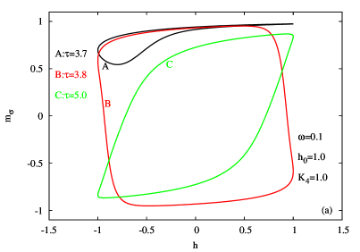
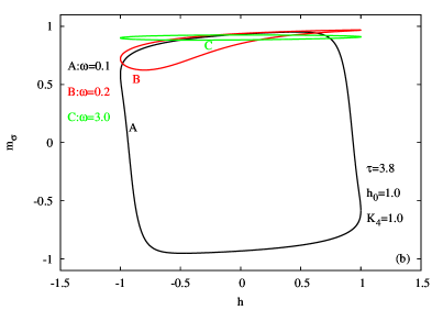
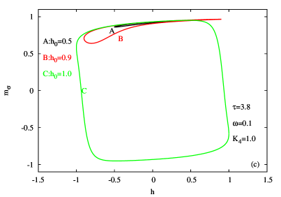
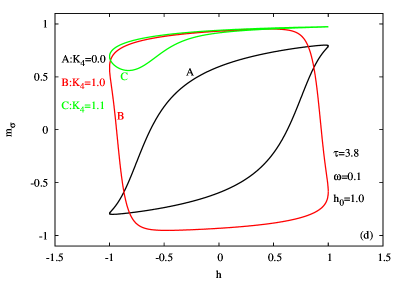
Figure 5: Hysteresis behavior of the IATM on a square lattice for changing (a) temperature, (b) frequency of the field, (c) amplitude of the field and (d) $K_{4}$, for selected values of Hamiltonian parameters.

Typical behaviors of the hysteresis loops with changing Hamiltonian parameters can be seen in Fig. 5. If we group hysteresis loops (as for the Ising model) as paramagnetic and ferromagnetic loops, we observe from Fig. 5 that, in the manner of transition between two kind of loops

• The effect of the rising temperature and amplitude of the field are similar, they give rise to transition from ferromagnetic loops to paramagnetic loops (see Fig. 5 (a) and (c))

• The effect of the rising frequency of the field and $K_{4}$ are similar, they give rise to transition from paramagnetic loops to ferromagnetic loops (see Fig. 5 (b) and (d)).

Rising temperature causes enhanced thermal fluctuations and the spins can follow the driving periodic magnetic field. The same reasoning holds for the rising amplitude of the field, since rising amplitude of the field means that more energy is supplied to the system from the magnetic field. These two mechanisms cause a transition from the ordered phase to the disordered phase. The reverse transition can be seen for the rising frequency of the field. After a specific frequency (which depends on all other Hamiltonian parameters), spins cannot follow the magnetic field, then ferromagnetic phase occurs. These facts have already been observed and explained for the dynamical Ising model [59]. For the IATM we observe from Fig. 5 (d) that rising $K_{4}$ can give rise to transition from the paramagnetic hysteresis loops to the ferromagnetic loops (compare loops labeled by A,B,C in Fig. 5 (d)). This behavior is consistent with the dynamic phase diagram which was depicted in Fig. 3 (d). As seen in Fig. 3 (d) while system is in the $DP_{3}$ phase for the temperature value of $\tau=3.8$, rising coupling constant $K_{4}$ gives rise to a transition to the $DP_{1}$ phase which has ferromagnetic hysteresis characteristics.

Note that there is not any significant difference between the observed hysteresis loops belonging to $DP_{2}$ and $DP_{3}$ phases. This is because both of the phases have $m_{\sigma}=0$. Thus the phases $DP_{2}$ and $DP_{3}$ could not be distinguished by hysteresis behaviors of order parameter $m_{\sigma}$. But the variation of the $m_{\sigma s}$ with magnetic field in one period may distinguish between these two phases. This loop may be called as hysteresis loop of $m_{\sigma s}$. In order to determine the response of this new order parameter (which is absent in the Ising model), we depict typical loops representing the phases $DP_{2},DP_{3}$ and $DP_{1}$ in Fig. 6. The other Hamiltonian parameter values are chosen as $\omega=0.1,h_{0}=0.1,K_{4}=0.2$. We can see from Fig. 3 (a) that, the curve labeled A in Fig. 6 represents the hysteresis loop of the phase $DP_{2}$, B represents the phase $DP_{3}$ and C and D correspond to the phase $DP_{1}$. First of all, the loop corresponds to the phase $DP_{2}$ (curve labeled by A) indeed a $m_{\sigma s}=0$ line, means that the order parameter $m_{\sigma s}=0$ does not respond to the varying magnetic field. As seen in Fig. 6, the order parameter $m_{\sigma s}$ starts to reply the changing magnetic field within the phase $DP_{3}$ (curve labeled B) and similar loop is valid for the phase $DP_{1}$ (curve labeled C). But one difference draws our attention: while the loop belonging to the phase $DP_{3}$ has one $m_{\sigma s}$ value for the zero field, the loop about the $DP_{1}$ phase has two very close but slightly different values of $m_{\sigma s}$ for the $h=0$ case. When the temperature is lowered, the loop like knot becomes dissolved and evolve into the loops like labeled D in Fig. 6. As a result, we can distinguish the phases $DP_{1},DP_{2}$ and $DP_{3}$ by looking at the hysteresis loops of the $m_{\sigma s}$ as explained above.

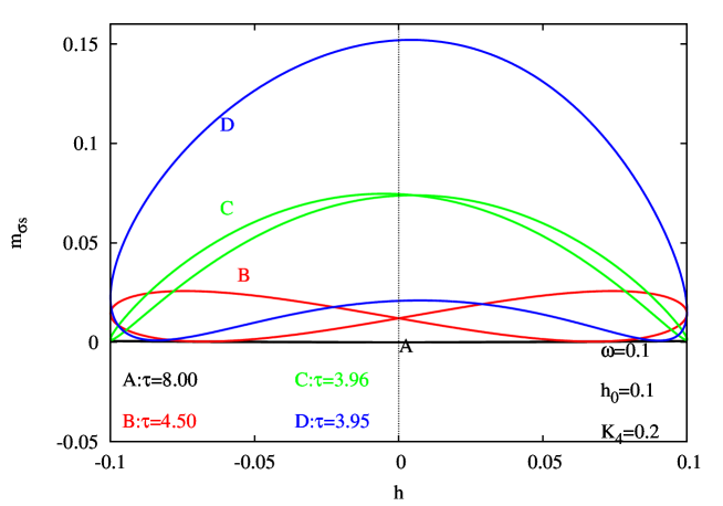
Figure 6: Variation of $m_{\sigma s}$ within the one period of the magnetic field for selected temperature values as $\tau=8.00,4.50,3.69,3.65$. Other values of the Hamiltonian parameters are fixed as $\omega=0.1,h_{0}=0.1,K_{4}=0.2$.

Lastly we want to elaborate the HLA properties of the system. For this aim we depict the contour plots of the HLA in ($\omega,K_{4}$) plane for selected values of $(h_{0},\tau)$ pair, which can be seen in Fig. 7. HLA of the dynamical Ising model has been widely inspected in the literature and the variation of the HLA with the frequency is well known. We want to determine the relation between $K_{4}$ and the HLA. This can be seen in contour plots for several cases. At first sight one difference is take our attention between the contour plots given in Fig. 7 (a)-(d). Rising $K_{4}$ with low frequencies result in lowering of the HLA in Fig. 7 (a) while the reverse relation holds in Figs. 7 (b)-(d). As seen in Fig. 3 (d), rising $K_{4}$ give rise to transition from the phase $DP_{3}$ to $DP_{1}$ and this transition causes depressed HLA. We cannot face this situation in Fig. 7 (b). For low frequencies, rising $K_{4}$ enhances the HLA. Again from Fig. 3 (d), we can see that, this variation cannot change the phase of the system, the system lies in the $DP_{3}$ phase and rising coupling $K_{4}$ between the two Ising models give rise to rising HLA. Same situation holds for Figs. 7 (c) and (d). The only difference is wider region of the $(K_{4},\omega)$ plane has big HLA due to the rising $h_{0}$ enlarges the region that have $DP_{2},DP_{3}$ regions.

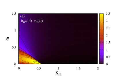
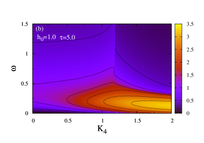
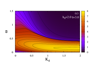
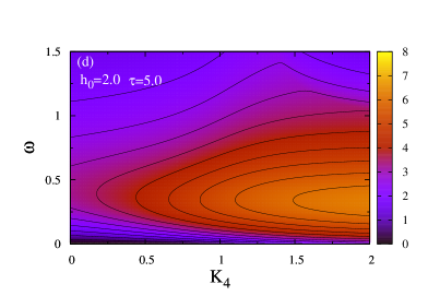
Figure 7: Contour plots of the HLA in ($\omega,K_{4}$) plane for selected values of $(h_{0},\tau)$ pair as (a) ($1.0,3.0$) (b) ($1.0,5.0$) (c) ($2.0,3.0$) (d) ($2.0,5.0$). Also contour lines added as starting with the value of $0.5$ and increment of $0.5$.

5 Conclusion

The phase diagrams and the hysteresis characteristics of the IATM has been investigated within the MFA with Glauber type of stochastic process. First, the phase diagrams of the model have been obtained in the $(\tau,K_{4})$ plane, by defining the possible dynamical phases of the system obtainable within the used approximation. The effect of the frequency and the amplitude of the periodic time dependent magnetic field on these diagrams has been investigated in detail.

To the hysteresis part of the work, since the effect of the Hamiltonian parameters on the hysteresis characteristics on the Isng model is well known and the effect of the Hamiltonian parameter $K_{4}$ on the hysteresis characteristics is mostly investigated. Dynamical phase transitions induced by changing $K_{4}$ shows itself on the hysteresis behaviors. These behaviors have been discussed in detail. Besides, the behavior of the order parameter of the IATM namely $m_{\sigma s}$ with the magnetic field has also been discussed. The relation between these hysteresis loops and possible phase transitions explored.

We hope that the results obtained in this work may be beneficial form both theoretical and experimental point of view.

References

- [1] J. Ashkin, E. Teller, Phys. Rev. 64 (1943) 178.
- [2] F. J. Wagner, J. Phys. C 5 (1972) L131 .
- [3] R. J. Baxter, 1982 Exactly Solved Models in Statistical Mechanics (London: Academic)
- [4] R.V. Ditzian, J.R. Banavar, G.S. Grest, and L.P. Kadanoff, Phys. Rev. B 22 (1980) 2542.
- [5] C. Fan, Phys. Lett. A 39 (1972) 136.
- [6] G.S. Grest and M. Widom, Phys. Rev. B 24 (1981) 6508.
- [7] P. Bak, P. Kleban, W.N. Unertel, J. Ochab, G. Akinci, N.C. Barlet, T.L. Einstein, Phys. Rev. Lett. 54 (1985) 1542.
- [8] M. Sluiter, Y. Kawazoe, Sci. Rep. Res. Inst. Tokohu Univ. A 40 (1995) 301.
- [9] M.S. Gronsleth, T.B. Nilssen, E.K. Dahl, E.B. Stiansen, C.M. Varma, A. Sudbo, 2009. arXiv:Cond-Mat/0806.2665v2.
- [10] C. Zhe, W. Ping, Z. Ying-Hong, Commun. Theor. Phys. 49 (2008) 525.
- [11] N.C. Bartelt, T.L. Einstein, L.T. Wille, Physica C 162–164 (1989) 871.
- [12] N.C. Bartelt, T.L. Einstein, L.T. Wille, Phys. Rev. B 40 (1989) 10759.
- [13] L.T. Wille, Phase Transitions 22 (1990) 225.
- [14] P. Arnold and Y. Zhang, Nucl. Phys. B 501 (1997) 803.
- [15] D. Bollé and P. Kozłowski, J. Phys. A 32 (1999) 8577.
- [16] V. S. Dotsenko, J. Phys. A 18 (1985) L241.
- [17] P. Calabrese, A. Celi, Pysical Review B 66 (2002) 184410.
- [18] P. Calabrese, E. V. Orlov, D. V. Pakhnin, A. I. Sokolov, Pysical Review B 70 (2004) 094425.
- [19] J. A. Plascak, F. C. Sá Barreto J. Phys. A: Math. Gen. 19 (1986) 2195.
- [20] N. Benayad, A. Benyoussef, N. Boccara, A. El Kenz, J . Phys. C: Solid State Phys. 21 (1988) 5747.
- [21] P. Arnold, Y. Zhang, Nuclear Physics B 501 (1997) 803
- [22] D. Jeziorek-Kniola , G. Musial, L. Debski , J. Rogiers, S. Dylak, Acta Physica Polonica A 121 (2012) 1105.
- [23] G. Musial, L. Debski, G. Kamieniarz, Phys. Rev. B 66 (2002) 012407.
- [24] G. Musial, Phys. Rev. B 69 (2004) 024407.
- [25] G. Kamieniarz, P. Kozlowski, Phys. Rev. E 55 (1997) 3724.
- [26] G. Musial, L. Debski, G. Kamieniarz, Phys. Stat. Sol. (b) 236 (2003) 441.
- [27] G. Musial, Phys. Stat. Sol. (b) 236 (2003) 486.
- [28] J. P. Santos, F.C. Sá Barreto, Physica A 421 (2015) 316.
- [29] M. Badehdah , S. Bekhechi , A. Benyoussef, M. Touzani Physica B 291 (2000) 394.
- [30] R. V. Ditzian, J. R. Banavar, G. S. Grest, L. P. Kadanoff, Phys. Rev. B 22 (1980) 2542.
- [31] J. R. Banavar, G. S. Grest, D. Jasnow, Phys. Rev. B 25 (1982) 4639.
- [32] A. M. Mariz, C.Tsallis, P. Fulco Phys. Rev. B 32 (1985) 6055.
- [33] A. S. Anjos, D. A. Moreira, A. M. Mariz, F. D. Nobre, F. A. da Costa, Phys. Rev. E 76 (2007) 041137.
- [34] A. M. Mariz, J. Phys. A: Math. Gen. 23 (1990) 979.
- [35] A. S. Anjos, I. S. Queiroz, A. M. Mariz, F. A. da Costa, Journal of Statistical Mechanics: Theory and Experiment (2009) P08002.
- [36] L. Bahmad, A. Benyoussef, H. Ez-Zahraouy, Phys. Stat. Sol. (b) 226 (2001) 403.
- [37] S. Bekhechi, A. Benyoussef, A. Elkenz, B. Ettaki, M. Loulidi, Physica A 264 (1999) 503.
- [38] S. Wiseman, E. Domany, Phys. Rev. E 48 (1993) 4080.
- [39] C.G. Bezerra, A.M. Mariz, J.M. de Araújo, F.A. da Costa, Physica A 292 (2001) 429.
- [40] J. Chahine, J. R. Drugowich de Felicio, N. Caticha, J. Phys. A: Math. Gen. 22 (1989) 1639.
- [41] J. X. Le, Z.R. Yang, Commun. Theor. Phys. 43 (2005) 841.
- [42] F.A.P. Piolho, F.A. da Costa, C.G. Bezerra, A.M. Mariz, Physica A 387 (2008) 1538.
- [43] J. X. Le, Z.R. Yang, Phys. Rev. E 68 (2003) 066105.
- [44] F. A. da Costa, M. J. de Oliveira, S. R. Salinas, Phys. Rev. B 36 (1987) 7163.
- [45] P. Pawlicki, J. Rogiers, Physica A 214 (1995) 277.
- [46] P. Pawlicki, J. Rogiers, G. Kamieniarz, J. Magn. Magn. Mater 140-144 (1995) 1479.
- [47] P. Pawlicki, G. Musial, G. Kamieniarz, J. Rogiers, Physica A 242 (1997) 281.
- [48] P. Pawlicki, G. Kamieniarz, L. Debski, Physica A 242 (1997) 290.
- [49] I. Dani, N. Tahiri, H. Ez-Zahraouy, A. Benyoussef, J. Magn. Magn. Mater 394 (2015) 27.
- [50] M. Loulidi, Phys. Rev. B 55 (1997) 11611.
- [51] M. Badehdah, S. Bekhechi, A. Benyoussef, B. Ettaki, Phys. Rev. B 59 (1999) 6250.
- [52] S. Bekhechi, A. Benyoussef , A. El kenz, B. Ettaki, M. Loulidi, Eur. Phys. J. B 18 (2000) 275.
- [53] M. J Martins, J R Drugowich de Felicio, J. Phys. A: Math. Gen. 21 (1988) 1117.
- [54] G. N. Murthy, Phys. Rev. B 36 (1987) 7166.
- [55] J.R. Drugowich de Felí cio , J. Chahine, N. Caticha, Physica A 321 (2003) 529.
- [56] G. S. Grest, M. Widom, Phys. Rev. B 24 (1981) 6508.
- [57] E. Fradkin, Phys. Rev. Lett. 53 (1984) 1967.
- [58] H. A. Ceccatto, J. Phys. A: Math. Gen. 24 (1991) 2829.
- [59] B.K. Chakrabarti, M. Acharyya, Rev. Modern Phys. 71 (1999) 847.
- [60] Q. Jiang, H.-N. Yang, G.-C. Wang, Physical Review B 52 (1995) 14911.
- [61] Y.-L. He, G.-C. Wang, Physical Review Letters 70 (1993) 2336.
- [62] W.Y. Lee, B.-Ch. Choi, J. Lee, C.C. Yao, Y.B. Xu, D.G. Hasko, J.A.C. Bland, Applied Physics Letters 74 (1999) 1609.
- [63] W.Y. Lee, B.-Ch. Choi, Y.B. Xu, J.A.C. Bland, Physical Review B 60 (1999) 10216.
- [64] T.A. Moore, J. Rothman, Y.B. Xu, J.A.C. Blanda, Journal of Applied Physics 89 (2001) 7018.
- [65] T. Tomé, M.J. de Oliveira, Phys. Rev. A 41 (1990) 4251.
- [66] M. Acharyya, Phys. Rev. E 58 (1998) 179.
- [67] M. Acharyya, Phys. Rev. E 59 (1999) 218.
- [68] B. Deviren, O. Canko, M. Keskin, Chinese Physics B 19 (2010) 050518.
- [69] R.J. Glauber, Journal of Mathematical Physics 4 (1963) 294.
- [70] R.B. Potts, Proc. Camb. Phil. Soc. 48 (1952) 106.
- [71] W. H. Press, S. A. Teukolsky, W. T. Vetterling, B. P. Flannery, Numerical Recipes in Fortran 90 (Third edition, Cambridge University Press, USA 2007)