The KdV, the Burgers, and the Whitham limit for
a spatially periodic Boussinesq model

Abstract.

We are interested in the Korteweg-de Vries (KdV), the Burgers, and the Whitham limit for a spatially periodic Boussinesq model with non-small contrast. We prove estimates between the KdV, the Burgers, and the Whitham approximation and true solutions of the original system which guarantee that these amplitude equations make correct predictions about the dynamics of the spatially periodic Boussinesq model over the natural time scales of the amplitude equations. The proof is based on Bloch wave analysis and energy estimates. The result is the first justification result of the KdV, the Burgers, and the Whitham approximation for a dispersive PDE posed in a spatially periodic medium of non-small contrast.

IADM, Universität Stuttgart, Pfaffenwaldring 57, 70569 Stuttgart Germany,
email: forename.lastname@mathematik.uni-stuttgart.de

1. Introduction

In the long wave limit there exists a zoo of amplitude equations which can be derived via multiple scaling analysis for various dispersive wave systems with conserved quantities. Generically, among these amplitude equations there are only three nonlinear ones which are independent of the small perturbation parameter, namely the Korteweg-de Vries (KdV) equation, the inviscid Burgers equation, and the Whitham system. It is the purpose of this paper to discuss the validity of these approximations for a spatially periodic Boussinesq model with non-small contrast.

1.1. The formal approximations in the spatially homogenous situation

The KdV equation occurs as an amplitude equation in the description of small spatially and temporally modulations of long waves in various dispersive wave systems. Examples are the water wave problem or equations from plasma physics, cf. [3]. For the Boussinesq equation

(1) $$\partial_{t}^{2}u(x,t)=\partial_{x}^{2}u(x,t)-\partial_{x}^{4}u(x,t)+\partial_{x}^{2}(u(x,t)^{2}),$$

with $x\in\mathbb{R}$, $t\in\mathbb{R}$, and $u(x,t)\in\mathbb{R}$, by the ansatz

(2) $$u(x,t)=\varepsilon^{2}A(X,T),$$

where $X=\varepsilon(x-t)$, $T=\varepsilon^{3}t$, $A(X,T)\in\mathbb{R}$, and $0<\varepsilon\ll 1$ a small perturbation parameter, the KdV equation

(3) $$\partial_{T}A=\frac{1}{2}\partial_{X}^{3}A-\frac{1}{2}\partial_{X}(A^{2})$$

can be derived by inserting (2) into (1) and by equating the coefficients in front of $\varepsilon^{6}$ to zero. This ansatz can be generalized to

(4) $$u(x,t)=\varepsilon^{\alpha}A(X,T),$$

where $X=\varepsilon(x-t)$, $T=\varepsilon^{1+\alpha}t$, and $A(X,T)\in\mathbb{R}$, with $\alpha>0$. For $\alpha>2$ the Airy equation $\partial_{T}A=\frac{1}{2}\partial_{X}^{3}A$ occurs. The KdV equation is recovered for $\alpha=2$, and for $\alpha\in(0,2)$ the inviscid Burgers equation

(5) $$\partial_{T}A=-\frac{1}{2}\partial_{X}(A^{2})$$

is obtained. There is another long wave limit which leads to an $\varepsilon$-independent non-trivial amplitude equation. With the ansatz

(6) $$u(x,t)=U(X,T),$$

where $X=\varepsilon x$, $T=\varepsilon t$, and $U(X,T)\in\mathbb{R}$, we obtain

(7) $$\partial_{T}^{2}U=\partial_{X}^{2}U+\partial_{X}^{2}(U^{2})$$

which can be written as a system of conservation laws

(8) $$\partial_{T}U=\partial_{X}V,\qquad\partial_{T}V=\partial_{X}U+\partial_{X}(U^{2}).$$

In the following both, (7) and (8), are called the Whitham system, cf. [26].

1.2. Justification by error estimates

Estimates that the formal KdV approximation and true solutions of the original system stay close together over the natural KdV time scale are a non-trivial task since solutions of order $\mathcal{O}(\varepsilon^{2})$ have to be shown to be existent on an $\mathcal{O}(1/\varepsilon^{3})$ time scale. For (1) an approximation result is formulated as follows.

Theorem 1.1.

Let $s\geq 0$ and let $A\in C([0,T_{0}],H^{5+s})$ be a solution of the KdV equation (3). Then there exist $\varepsilon_{0}>0$ and $C>0$ such that for all $\varepsilon\in(0,\varepsilon_{0})$ we have solutions $u$ of (1) with

$$\sup_{t\in[0,T_{0}/\varepsilon^{3}]}\|u(\cdot,t)-\varepsilon^{2}A(\varepsilon(\cdot-t),\varepsilon^{3}t)\|_{H^{1+s}}\leq C\varepsilon^{7/2}.$$

There are two fundamentally different approaches to prove such an approximation result. For analytic initial conditions of the KdV equation a Cauchy-Kowalevskaya based approach can be chosen, see [19] with the comments given in [22] for the water wave problem. Working in spaces of analytic functions gives some artificial smoothing which allows to gain the missing order w.r.t. $\varepsilon$ between the inverse of the amplitude of $\mathcal{O}(\varepsilon^{2})$ and the time scale of $\mathcal{O}(1/\varepsilon^{3})$ via the derivative in front of the nonlinear terms in the KdV equation. This approach is very robust and works without a detailed analysis of the underlying problem, cf. [5] for another example, but gives not optimal results.

For initial conditions in Sobolev spaces the underying idea to gain such estimates is conceptually rather simple, namely the construction of a suitable chosen energy which include the terms of order $\mathcal{O}(\varepsilon^{2})$ in the equation for the error, such that for the energy finally $\mathcal{O}(\varepsilon^{3}t)$ growth rates occur. However, the method is less robust since for every single original system a different energy occurs and the major difficulty is the construction of this energy. Estimates that the formal KdV approximation and true solutions of the different formulations of the water wave problem stay close together over the natural KdV time scale have been shown for instance in [10, 23, 24, 1, 14] using this approach. Another example is the justification of the KdV approximation for modulations of periodic waves in the NLS equation, cf. [6]. For (1) the energy approach is rather short and very instructive for the subsequent analysis. Therefore, we recall it in Section 2.

Interestingly, it turns out that the proofs given for the KdV approximations transfer more or less line for line into proofs for the justification of the inviscid Burgers equation and of the Whitham system. Since only the scaling has to be adapted, whenever a KdV approximation result holds also an inviscid Burgers and Whitham approximation result can be established. This will be explained in detail in Section 2.

As above such approximation results are a non-trivial task since solutions of order $\mathcal{O}(\varepsilon^{\alpha})$ have to be shown to be existent on an $\mathcal{O}(\varepsilon^{1+\alpha})$ time scale. For the inviscid Burgers equation the formulation of the approximation result goes along the lines of Theorem 1.1. However, due to the notational complexity in achieving in general the estimates for the residual (the terms which do not cancel after inserting the approximation into (9)), in Remark 2.3 we restrict ourselves to the case $\alpha=1$.

Theorem 1.2.

Let $s\geq 0$, $\alpha=1$ and let $A\in C([0,T_{0}],H^{3+s})$ be a solution of the inviscid Burgers equation (5). Then there exist $\varepsilon_{0}>0$ and $C>0$ such that for all $\varepsilon\in(0,\varepsilon_{0})$ we have solutions $u$ of (1) with

$$\sup_{t\in[0,T_{0}/\varepsilon^{2}]}\|u(\cdot,t)-\varepsilon A(\varepsilon(\cdot-t),\varepsilon^{2}t)\|_{H^{1+s}}\leq C\varepsilon^{(3+2\alpha)/2}.$$

Since for the Whitham approximation solutions of order $\mathcal{O}(1)$ are considered some smallness condition is needed such that the used energy allows us to estimate the associated Sobolev norm.

For (1) a possible Whitham approximation result is formulated as follows.

Theorem 1.3.

Let $s\geq 0$. There exists a $C_{1}>0$ such that the following holds. Let $U\in C([0,T_{0}],H^{3+s})$ be a solution of (7) with

$$\sup_{T\in[0,T_{0}]}\|U(\cdot,T)\|_{H^{3+s}}\leq C_{1}.$$

Then there exist $\varepsilon_{0}>0$ and $C>0$ such that for all $\varepsilon\in(0,\varepsilon_{0})$ we have solutions $u$ of (1) with

$$\sup_{t\in[0,T_{0}/\varepsilon]}\|u(\cdot,t)-U(\varepsilon\cdot,\varepsilon t)\|_{H^{1+s}}\leq C\varepsilon^{3/2}.$$

The Whitham system for the water wave problem coincides with the shallow water wave equations which have been justified for the water wave problem without surface tension in [20, 17]. A Whitham approximation result that the periodic wave trains of the NLS equation are approximated by the Whitham system can be found in [13].

1.3. The spatially periodic situation

The last years have seen some first attempts to justify the KdV equation in periodic media. It has been justified in [17] for the water wave problem over a periodic bottom in the KdV scaling, i.e., with long wave oscillations of the bottom of magnitude $\mathcal{O}(\varepsilon^{2})$ varying on a spatial scale of order $\mathcal{O}(\varepsilon^{-1})$. The same result can be found in [9] where general bottom topographies of small amplitude have been handled. The result is based on [8] where other amplitude systems have been justified. This situation can be handled as perturbation of the spatially homogeneous case.

In case of oscillations of the bottom of magnitude $\mathcal{O}(1)$ varying on a spatial scale of order $\mathcal{O}(1)$, no approximation result can be found in the existing literature. As a first attempt to solve this question for the water wave problem we consider a spatially periodic Boussinesq equation

(9) $$\partial_{t}^{2}u(x,t)= \partial_{x}(a(x)\partial_{x}u(x,t))$$

$$-\partial_{x}^{2}(b(x)\partial_{x}^{2}u(x,t))+\partial_{x}(c(x)\partial_{x}(u(x,t)^{2})),$$

with $x\in\mathbb{R}$, $t\geq 0$, $u(x,t)\in\mathbb{R}$, and smooth $x$-dependent $2\pi$-spatially periodic coefficients $a$, $b$, and $c$ satisfying

$$\inf_{x\in\mathbb{R}}a(x)>0\quad\textrm{and}\quad\inf_{x\in\mathbb{R}}b(x)>0.$$

For this equation we derive the KdV equation by making a Bloch mode expansion of (9). The KdV approximation describes the modes which in Figure 1 are contained in the circles. We prove an approximation result which is formulated in Theorem 5.1. It guarantees that the KdV equation makes correct predictions about the dynamics of the spatially periodic Boussinesq model (9) over the natural KdV time scale. The presented result is the first justification result of the KdV approximation for a dispersive nonlinear PDE posed in a spatially periodic medium of non-small contrast. For linear systems this limit has been considered independently in [11, 12].

In order to make the residual small an improved approximation has to be constructed. Since this construction is not the main purpose of this paper we additionally assume

(SYM) the coefficient functions

$$a=a(x),\quad b=b(x),\quad\textrm{and}\quad c=c(x)\quad\textrm{are even w.r.t. }x.$$

As in the spatially homogeneous situation it turns out that the proof given for the KdV approximation transfers more or less line for line into proofs for the justification of the approximation via the inviscid Burgers equation and of the Whitham system. The associated approximation results are formulated in Theorem 5.2 and Theorem 5.3.

The paper was originally intended as the next step in generalizing a method which has been developed in [7] for the justification of the KdV approximation in situations when the KdV modes are resonant to other long wave modes. The method had already successfully been applied in justifying the KdV approximation for the poly-atomic FPU problem in [4]. The qualitative difference in justifying the KdV equation for the spatially periodic Boussinesq equation in contrast to [7, 4] is that for fixed Bloch respectively Fourier wave number the presented problem is infinite dimensional. [7, 4] corresponds to the middle panel of Figure 1 where the spatially periodic Boussinesq equation corresponds to the right panel of Figure 1. As a consequence the normal form transform which is a major part of the proofs of [7, 4] would be more demanding from an analytic point of view. In the justification of the Whitham system with the approach of [7, 4] infinitely many normal form transforms have to be performed [15].

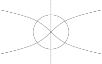
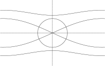
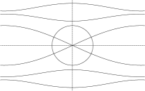
Figure 1. The left panel shows the curves of eigenvalues over the Fourier wave numbers as it appears for the water wave problem [10, 23, 24, 1, 17, 14]. The middle panel shows the finitely many curves of eigenvalues as they appear for instance for the poly-atomic FPU system [7, 4]. The right panel shows the infinitely many curves of eigenvalues over the Bloch wave numbers as it appears for the spatially periodic Boussinesq model (9), the water wave problem over a periodic bottom topography, or for the linearization around a periodic wave in dispersive systems. Since the Fourier transform of $\varepsilon^{2}A(\varepsilon x)$ is given by $\varepsilon^{2}\varepsilon^{-1}\widehat{A}(x/\varepsilon)$ the KdV equations describe the modes at the wave numbers $k=0$ with the vanishing eigenvalues which are contained in the circles. One of the two curves in the circle describes wave packets moving to the left, the other curve wave packets moving to the right.

Interestingly, for the spatially periodic Boussinesq equation (9) there exists an energy in physical space which allowed us to incorporate the normal form transforms into the energy estimates. This energy approach is presented in the following.

Notation. Constants which can be chosen independently of the small perturbation parameter $0<\varepsilon\ll 1$ are denoted with the same symbol $C$. We write $\int$ for $\int_{-\infty}^{\infty}$. The Fourier transform of a function $u$ is denoted with $\widehat{u}$. The Bloch transform of a function $u$ is denoted with $\widetilde{u}$ and this tool is recalled in Appendix C. We introduce the norm $\|\cdot\|_{L^{2}_{s}}$ by

$$\|\widehat{u}\|_{L^{2}_{s}}^{2}=\int|\widehat{u}(k)|^{2}(1+k^{2})^{s}dk$$

and define the Sobolev norm $\|u\|_{H^{s}}=\|\widehat{u}\|_{L^{2}_{s}}$, but use also equivalent versions.

Acknowledgement. The authors are grateful to Florent Chazel for helping us to understand the existing literature. Moreover, we would like to thank Martina Chirilus-Bruckner for a number of helpful discussions. The paper is partially supported by the Deutsche Forschungsgemeinschaft (DFG) under the grant Schn520/9-1.

2. The spatially homogeneous case

It is the goal of this section to give a simple proof for Theorem 1.1, Theorem 1.2, and Theorem 1.3 using the energy method. The proof will be the basis of the subsequent analysis. All three cases can be handled with the same approach.

The residual

$$\mathrm{Res}(u)=-\partial_{t}^{2}u(x,t)+\partial_{x}^{2}u(x,t)-\partial_{x}^{4}u(x,t)+\partial_{x}^{2}(u(x,t)^{2})$$

quantifies how much a function $u$ fails to satisfy the Boussinesq model (1). For the KdV approximation (2) abbreviated with $\varepsilon^{2}\Psi$ we find

$$\mathrm{Res}(\varepsilon^{2}\Psi) = -\varepsilon^{4}c^{2}\partial_{X}^{2}A-2\varepsilon^{6}\partial_{T}\partial_{X}A-\varepsilon^{8}\partial_{T}^{2}A$$

$$+\varepsilon^{4}\partial_{X}^{2}A-\varepsilon^{6}\partial_{X}^{4}A+\varepsilon^{6}\partial_{X}^{2}(A^{2})$$

$$= -\varepsilon^{8}\partial_{T}^{2}A$$

if we choose $A$ to satisfy the KdV equation (3). Therefore, we have

Lemma 2.1.

Let $s\geq 0$ and let $A\in C([0,T_{0}],H^{5+s})$ be a solution of the KdV equation (3). Then there exist $\varepsilon_{0}>0$, $C_{\rm res}$ such that for all $\varepsilon\in(0,\varepsilon_{0})$ we have

$$\sup_{t\in[0,T_{0}/\varepsilon^{3}]}\|\partial_{x}^{s-1}\mathrm{Res}(\varepsilon^{2}\Psi(\cdot,t,\varepsilon))\|_{L^{2}}\leq C_{\rm res}\varepsilon^{(13+2s)/2}.$$

Proof.

Using the KdV equation allows us to write

$$4\partial_{T}^{2}A = -2\partial_{T}(\partial_{X}^{3}A+\partial_{X}(A^{2}))=-2(\partial_{X}^{3}\partial_{T}A+2\partial_{X}(A\partial_{T}A))$$

$$= \partial_{X}^{3}(\partial_{X}^{3}A+\partial_{X}(A^{2}))+2\partial_{X}(A(\partial_{X}^{3}A+\partial_{X}(A^{2}))).$$

This shows that $A(\cdot,T)\in H^{6}$ is necessary to estimate the residual in $L^{2}$. The formal error of order $\mathcal{O}(\varepsilon^{8})$ is reduced by a factor $\varepsilon^{-1/2}$ due to the scaling properties of the $L^{2}$-norm. Moreover, due to the representation of $\partial_{T}^{2}A$ as a spatial derivative, below, we can apply $\partial_{x}^{-1}=\varepsilon^{-1}\partial_{X}^{-1}$ to the residual terms which however loses another factor $\varepsilon^{-1}$. ∎

Similarly, for the Whitham approximation (6) abbreviated with $\varepsilon^{2}\Psi$ we find $\textrm{Res}(\Psi)=-\varepsilon^{4}\partial_{X}^{4}U$ if we choose $U$ to satisfy the Whitham system (7). Hence, for an estimate in $L^{2}$ we need $U\in H^{4}$. Exactly as above we have

Lemma 2.2.

Let $s\geq 0$ and let $A\in C([0,T_{0}],H^{3+s})$ be a solution of the Whitham system (7). Then there exist $\varepsilon_{0}>0$, $C_{\rm res}$ such that for all $\varepsilon\in(0,\varepsilon_{0})$ we have

$$\sup_{t\in[0,T_{0}/\varepsilon]}\|\partial_{x}^{s-1}\mathrm{Res}(\Psi(\cdot,t,\varepsilon))\|_{L^{2}}\leq C_{\rm res}\varepsilon^{(5+2s)/2}.$$

Remark 2.3.

For the inviscid Burgers equation the residual becomes too large with the simple ansatz (2). However, by adding higher order terms to the approximation (2), with a slight abuse of notation this approximation is again called $\varepsilon^{\alpha}\Psi$, one can always achieve

$$\sup_{t\in[0,T_{0}/\varepsilon^{1+\alpha}]}\|\mathrm{Res}(\varepsilon^{\alpha}\Psi(\cdot,t,\varepsilon))\|_{L^{2}}\leq C_{\rm res}\varepsilon^{(7+4\alpha)/2}$$

and

$$\sup_{t\in[0,T_{0}/\varepsilon^{1+\alpha}]}\|\partial_{x}^{-1}\mathrm{Res}(\varepsilon^{\alpha}\Psi(\cdot,t,\varepsilon))\|_{L^{2}}\leq C_{\rm res}\varepsilon^{(5+4\alpha)/2}.$$

See Appendix A where we prove these estimates for $\alpha=1$ and explain that the number of additional terms goes to infinity for $\alpha\to 0$ and $\alpha\to 2$.

From this point on the remaining estimates can be handled exactly the same. The case $\alpha=0$ corresponds to the Whitham approximation and the case $\alpha=2$ to the KdV approximation. The difference $\varepsilon^{(3+2\alpha)/2}R=u-\varepsilon^{\alpha}\Psi$ satisfies

(10) $$\partial_{t}^{2}R=\partial_{x}^{2}R-\partial_{x}^{4}R+2\varepsilon^{\alpha}\partial_{x}^{2}(\Psi R)+\varepsilon^{(3+2\alpha)/2}\partial_{x}^{2}(R^{2})+\varepsilon^{-(3+2\alpha)/2}\mathrm{Res}(\varepsilon^{2}\Psi).$$

We multiply the error equation (10) with $-\partial_{t}\partial_{x}^{-2}R$ which is defined via its Fourier transform w.r.t. $x$, namely via $\widehat{\partial_{x}^{-1}R}(k)=\frac{1}{ik}\widehat{R}(k)$, integrate it w.r.t. $x$, and find

$$-\int(\partial_{t}\partial_{x}^{-2}R)\partial_{t}^{2}Rdx = \partial_{t}\int(\partial_{t}\partial_{x}^{-1}R)^{2}dx/2,$$

$$-\int(\partial_{t}\partial_{x}^{-2}R)\partial_{x}^{2}Rdx = -\partial_{t}\int R^{2}dx/2,$$

$$\int(\partial_{t}\partial_{x}^{-2}R)\partial_{x}^{4}Rdx = -\partial_{t}\int(\partial_{x}R)^{2}dx/2,$$

$$-\int(\partial_{t}\partial_{x}^{-2}R)\partial_{x}^{2}(\Psi R)dx = -\int(\partial_{t}R)\Psi Rdx$$

$$= -\partial_{t}\int\Psi R^{2}dx/2+\varepsilon\int(\partial_{\tau}\Psi)R^{2}dx,$$

$$-\int(\partial_{t}\partial_{x}^{-2}R)\partial_{x}^{2}(R^{2})dx = -\int(\partial_{t}R)R^{2}dx=-\frac{1}{3}\partial_{t}\int R^{3}dx,$$

$$-\int(\partial_{t}\partial_{x}^{-2}R)\mathrm{Res}(\varepsilon^{2}\Psi)dx = \int(\partial_{t}\partial_{x}^{-1}R)\partial_{x}^{-1}\mathrm{Res}(\varepsilon^{2}\Psi)dx.$$

We can estimate

$$|\int(\partial_{t}\partial_{x}^{-1}R)\partial_{x}^{-1}\mathrm{Res}(\varepsilon^{2}\Psi)dx| \leq \|\partial_{t}\partial_{x}^{-1}R\|_{L^{2}}\|\partial_{x}^{-1}\mathrm{Res}(\varepsilon^{2}\Psi)\|_{L^{2}},$$

$$|\int(\partial_{\tau}\Psi)R^{2}dx| \leq \|\partial_{\tau}\Psi\|_{L^{\infty}}\|R\|_{L^{2}}^{2}.$$

For the energy

$$E = \int(\partial_{t}\partial_{x}^{-1}R)^{2}+R^{2}+(\partial_{x}R)^{2}+2\varepsilon^{\alpha}\Psi R^{2}+2\varepsilon^{(3+2\alpha)/2}R^{3}/3dx$$

the following holds. In case $\alpha>0$ we have that for all $M>0$ there exist $C_{1},\varepsilon_{1}>0$ such that for all $\varepsilon\in(0,\varepsilon_{1})$ we have

$$\|R\|_{H^{1}}\leq C_{1}E^{1/2}$$

as long as $E\leq M$. In case $\alpha=0$ the energy $E$ is an upper bound for the squared $H^{1}$-norm for $\|\Psi\|_{L^{\infty}}$ sufficiently small, but independent of $0<\varepsilon\ll 1$. Therefore, $E$ satisfies the inequality

$$\frac{dE}{dt} \leq C\varepsilon^{1+\alpha}E+C\varepsilon^{(3+2\alpha)/2}E^{3/2}+C\varepsilon^{1+\alpha}E^{1/2}$$

$$\leq 2C\varepsilon^{1+\alpha}E+C\varepsilon^{(3+2\alpha)/2}E^{3/2}+C\varepsilon^{1+\alpha},$$

with a constant $C$ independent of $\varepsilon\in(0,\varepsilon_{1})$. Under the assumption that $C\varepsilon^{1/2}E^{1/2}\leq 1$ we obtain

$$\frac{dE}{dt}\leq(2C+1)\varepsilon^{1+\alpha}E+C\varepsilon^{1+\alpha}.$$

Gronwall’s inequality immediately gives the bound

$$\sup_{t\in[0,T_{0}/\varepsilon^{1+\alpha}]}E(t)=CT_{0}e^{(2C+1)T_{0}}=:M=\mathcal{O}(1).$$

Finally choosing $\varepsilon_{2}>0$ so small that $C\varepsilon_{2}^{1/2}M^{1/2}\leq 1$ gives the required estimate for all $\varepsilon\in(0,\varepsilon_{0})$ with $\varepsilon_{0}=\min(\varepsilon_{1},\varepsilon_{2})>0$ in all three cases.

Remark 2.4.

The Boussinesq model (1) is a semilinear dispersive system and so there is the local existence and uniqueness of solutions. The variation of constant formula associated to the first order system for the variables $u$ and $\partial_{t}(\partial_{x}^{4}-\partial_{x}^{2})^{-1/2}u$ is a contraction in the space $C([-T_{*},T_{*}],H^{\theta}\times H^{\theta})$ for every $\theta>1/2$ if $T_{*}>0$ is sufficiently small. The local existence and uniqueness of solutions combined with the previous estimates for instance yields the existence and uniqueness of solutions for all $t\in[0,T_{0}/\varepsilon^{3}]$ in the KdV case and all $t\in[0,T_{0}/\varepsilon]$ in the Whitham case.

3. Derivation of the amplitude equations

In this section we come back to the spatially periodic situation. The derivation of the amplitude equations is less obvious than in the spatially homogeneous case. In order to derive the amplitude equations we expand (9) into the eigenfunctions of the linear problem. As in [2] after this expansion we are back in the spatially homogeneous set-up except that Fourier transform has been replaced by the Bloch transform.

3.1. Spectral properties

The linearized problem

(12) $$\partial_{t}^{2}u(x,t)=\partial_{x}(a(x)\partial_{x}u(x,t))-\partial_{x}^{2}(b(x)\partial_{x}^{2}u(x,t))$$

is solved by so called Bloch modes

$$u(x,t)=w(x)e^{ilx}e^{i\omega t},$$

with $w$ being $2\pi$-periodic w.r.t. $x$ satisfying

$$-(\partial_{x}+il)(a(x)(\partial_{x}+il)w(x))+(\partial_{x}+il)^{2}(b(x)(\partial_{x}+il)^{2}w(x))=\omega^{2}w(x).$$

The left hand side defines a self-adjoint elliptic operator $L_{l}(\partial_{x}):H^{\theta+4}\to H^{\theta}$. Hence, for fixed $l$ there exists a countable set of eigenvalues $\lambda_{n}(l)$, with $n\in\mathbb{N}$, ordered such that $\lambda_{n+1}(l)\geq\lambda_{n}(l)$, with associated eigenfunctions $w_{n}(x,l)$.

Lemma 3.1.

For $l=0$ the operator $L_{0}(\partial_{x})$ possesses the simple eigenvalue $\lambda_{1}(0)=0$ associated to the eigenfunction $\widetilde{w}_{1}(0,x)=1$.

Proof. Obviously we have $L_{0}(\partial_{x})1=0$. Moreover, we have

$$(w,L_{0}(\partial_{x})w)_{L^{2}}=\int_{-1/2}^{1/2}a(x)(\partial_{x}w(x))^{2}dx+\int_{-1/2}^{1/2}b(x)(\partial_{x}^{2}w(x))^{2}dx\geq 0.$$

Hence $L_{0}(\partial_{x})w=0$ implies $\partial_{x}w=0$. From the $2\pi$-periodicity it follows $w=const$. Hence $\lambda_{1}(0)=0$ is a simple eigenvalue. ∎

It is well known that the curves $l\mapsto\lambda_{n}(l)$ and $l\mapsto\widetilde{w}_{n}(l,\cdot)$ are smooth w.r.t. $l$ for simple eigenvalues. Hence, there exists a $\delta_{0}>0$ such that for $l\in[-\delta_{0},\delta_{0}]$ the smallest eigenvalue $\lambda_{1}(l)$ is separated from the rest of the spectrum. Since $L_{l}(\partial_{x})$ is self-adjoint and positive-definite for all $l$ we have $\lambda_{1}(l)\geq 0$ for all $l$. In the KdV equation only odd and in the Whitham system only even spatial derivatives occur. This is a consequence of the following lemma.

Lemma 3.2.

The curve $l\mapsto\lambda_{1}(l)$ for $l\in[-\delta_{0},\delta_{0}]$ is an even real-valued function. The associated eigenfunctions satisfy $\widetilde{w}_{1}(l,x)=\overline{\widetilde{w}_{1}(-l,x)}$. Under the assumption that the coefficient functions $a$ and $b$ are even, the eigenfunctions possess an expansion

$$\widetilde{w}_{1}(l,x)=\sum_{j=0}^{\infty}(il)^{j}g_{j}(x),$$

with $g_{0}(x)=1$, $\int_{0}^{2\pi}g_{j}(x)dx=0$ for $j\geq 1$,

$$g_{2j}(x)=g_{2j}(-x)\in\mathbb{R}\qquad\textrm{and}\qquad g_{2j+1}(x)=-g_{2j+1}(-x)\in\mathbb{R}.$$

Proof. The first two statements follow from the fact that for fixed $l$ the operator $L_{l}(\partial_{x})$ is self-adjoint and from the fact that (9) is a real problem. For $(il)^{0}$ we obtain

$$-\partial_{x}(a(x)\partial_{x}g_{0}(x))+\partial_{x}^{2}(b(x)\partial_{x}^{2}g_{0}(x))=0$$

which is, as we already know, uniquely been solved by $g_{0}(x)=1$. For $(il)^{1}$ we obtain

$$-\partial_{x}(a(x)\partial_{x}g_{1}(x))+\partial_{x}^{2}(b(x)\partial_{x}^{2}g_{1}(x))-\partial_{x}a(x)=0.$$

The term $\partial_{x}a(x)$ is odd. The subspace of odd functions is invariant for the differential operator $L_{0}(\partial_{x})=-\partial_{x}(a(x)(\partial_{x}\cdot)+\partial_{x}^{2}(b(x)\partial_{x}^{2}\cdot)$. Moreover in this subspace its spectrum is bounded away from zero such that this equation possesses a unique odd solution $g_{1}=g_{1}(x)$. For $(il)^{2}$ we obtain

$$-\partial_{x}(a(x)\partial_{x}g_{2}(x))+\partial_{x}^{2}(b(x)\partial_{x}^{2}g_{2}(x))+1+f_{2}(x)=1$$

with $f_{2}(x)$ an even function depending on $a$, $b$, $g_{0}$, and $g_{1}$ and possessing vanishing mean value. In the subspace of vanishing mean value the differential operator $L_{0}(\partial_{x})$ possesses spectrum which is bounded away from zero such that this equation possesses a unique even solution $g_{2}=g_{2}(x)$. With the same arguments the next orders with the stated properties can be computed. The convergence of the series in a neighborhood of $l=0$ in $H^{\theta}$ for every $\theta\geq 0$ follows from the smoothness of the curve of simple eigenfunctions w.r.t. $l$ and the smoothness of the coefficient functions $a$, $b$, and $c$ w.r.t. $x$. ∎

The KdV equation, the inviscid Burgers equation, and the Whitham system describe the modes associated to the curve $\lambda_{1}$ close to $l=0$. Therefore, in order to derive these amplitude equations we consider the Bloch transform

$$u(x,t)=\int_{-1/2}^{1/2}\widetilde{u}(l,x,t)e^{ilx}dx$$

of (9), namely

(13) $$\partial_{t}^{2}\widetilde{u}(l,x,t)=-L_{l}(\partial_{x})\widetilde{u}(l,x,t)+N_{l}(\partial_{x})(\widetilde{u})(l,x,t)$$

where

$$N_{l}(\partial_{x})(\widetilde{u})(l,x,t)=(\partial_{x}+il)(c(x)(\partial_{x}+il)\int_{-1/2}^{1/2}\widetilde{u}(l-m,x,t)\widetilde{u}(m,x,t)dm.$$

Then we make the ansatz

$$\widetilde{u}(l,x,t)=\chi_{[-\delta_{0}/2,\delta_{0}/2]}(l)\widetilde{u}_{1}(l,t)\widetilde{w}_{1}(l,x)+\widetilde{v}(l,x,t)$$

with

$$\int_{0}^{2\pi}\overline{\widetilde{w}_{1}(l,x)}\widetilde{v}(l,x,t)dx=0$$

for $l\in[-\delta_{0}/2,\delta_{0}/2]$ and find

$$\partial_{t}^{2}\widetilde{u}_{1}(l,t) = -\lambda_{1}(l)\widetilde{u}_{1}(l,t)+P_{c}(l)N_{l}(\partial_{x})(\widetilde{u})(l,t),$$

$$\partial_{t}^{2}\widetilde{v}(l,x,t) = -L_{l}(\partial_{x})\widetilde{v}(l,x,t)+P_{s}(l)N_{l}(\partial_{x})(\widetilde{u})(l,x,t),$$

where

$$(P_{c}\widetilde{u})(l,t) = \frac{1}{2\pi}\chi_{[-\delta_{0}/2,\delta_{0}/2]}(l)\int_{0}^{2\pi}\overline{\widetilde{w}_{1}(l,x)}\widetilde{u}(l,x,t)dx,$$

$$(P_{s}\widetilde{u})(l,x,t) = \widetilde{u}(l,x,t)-(P_{c}\widetilde{u})(l,t){w}_{1}(l,x).$$

All amplitude equations which we have in mind can be derived in a very similar way. They describe the evolution of the $\widetilde{u}_{1}$ modes which are concentrated in an $\mathcal{O}(\varepsilon)$ neighborhood of the Bloch wave number $l=0$. In all three cases we make an ansatz

(14) $$\widetilde{u}_{1}(l,t)=\varepsilon^{-1}\varepsilon^{\alpha}\chi_{[-\delta_{0}/4,\delta_{0}/4]}(\frac{l}{\varepsilon})\widehat{A}(\frac{l}{\varepsilon},\varepsilon^{1+\alpha}t)e^{ilct}$$

with $\alpha=2$ and $c>0$ for the KdV approximation, $\alpha\in(0,2)$ and $c>0$ for the inviscid Burgers approximation, and $\alpha=0$ and $c=0$ for the Whitham approximation, cf. the text below Figure 1. The amplitude $\widehat{A}$ will be defined in Fourier space and the cut-off function $\chi_{[-\delta_{0}/4,\delta_{0}/4]}(\frac{l}{\varepsilon})$ allows to transfer $\widehat{A}$ into Bloch space. In the following we use the abbreviation

(15) $$\widetilde{A}(\frac{l}{\varepsilon},\varepsilon^{1+\alpha}t)=\chi_{[-\delta_{0}/4,\delta_{0}/4]}(\frac{l}{\varepsilon})\widehat{A}(\frac{l}{\varepsilon},\varepsilon^{1+\alpha}t).$$

For each of the three approximations we have to derive the associated amplitude equation and to compute and estimate the residual terms

$$\textrm{Res}(\widetilde{u})(l,x,t) = -\partial_{t}^{2}\widetilde{u}(l,x,t)-L_{l}(\partial_{x})\widetilde{u}(l,x,t)+N_{l}(\partial_{x})(\widetilde{u})(l,x,t).$$

3.2. Derivation of the KdV and the inviscid Burgers equation

The amplitude equations which we have in mind have derivatives in front of the nonlinear terms. Hence before deriving these equations we need to prove a number of properties about the nonlinear terms. We introduce kernels $s_{11}^{1}(l,l-m,m),\ldots,s_{vv}^{v}(l,l-m,m)$ by

$$(P_{c}N_{l}(\partial_{x})(\widetilde{u}))(l,t) = \int_{-1/2}^{1/2}s_{11}^{1}(l,l-m,m)\widetilde{u}_{1}(l-m,t)\widetilde{u}_{1}(m,t)dm$$

$$+\int_{-1/2}^{1/2}s_{1v}^{1}(l,l-m,m)\widetilde{u}_{1}(l-m,t)\widetilde{v}(m,x,t)dm$$

$$+\int_{-1/2}^{1/2}s_{v1}^{1}(l,l-m,m)\widetilde{v}(l-m,x,t)\widetilde{u}_{1}(m,t)dm$$

$$+\int_{-1/2}^{1/2}s_{vv}^{1}(l,l-m,m)\widetilde{v}(l-m,x,t)\widetilde{v}(m,x,t)dm$$

and

$$(P_{s}N_{l}(\partial_{x})(\widetilde{u}))(l,x,t) = \int_{-1/2}^{1/2}s_{11}^{v}(l,l-m,m)\widetilde{u}_{1}(l-m,t)\widetilde{u}_{1}(m,t)dm$$

$$+\int_{-1/2}^{1/2}s_{1v}^{v}(l,l-m,m)\widetilde{u}_{1}(l-m,t)\widetilde{v}(m,x,t)dm$$

$$+\int_{-1/2}^{1/2}s_{v1}^{v}(l,l-m,m)\widetilde{v}(l-m,x,t)\widetilde{u}_{1}(m,t)dm$$

$$+\int_{-1/2}^{1/2}s_{vv}^{v}(l,l-m,m)\widetilde{v}(l-m,x,t)\widetilde{v}(m,x,t)dm.$$

For the derivation of the KdV and the Burgers equation we need

Lemma 3.3.

We have

$$|s_{11}^{1}(l,l-m,m)-\nu_{2}l^{2}|\leq C|l|(l^{2}+(l-m)^{2}+m^{2}),$$

where

(16) $$\nu_{2}=-\frac{1}{2\pi}\int_{0}^{2\pi}c(x)(1+\partial_{x}g_{1}(x))^{2}dx.$$

Proof. Due to Lemma 3.2 we have

(17) $$\widetilde{w}_{1}(l,x)=1+ilg_{1}(x)+\mathcal{O}(l^{2})$$

where $g_{1}(x)\in\mathbb{R}$ with $\int_{0}^{2\pi}g_{1}(x)dx=0$. This expansion yields

$$2\pi s_{11}^{1}(l,l-m,m)$$

$$= \int_{0}^{2\pi}\overline{\widetilde{w}_{1}(l,x)}(\partial_{x}+il)(c(x)(\partial_{x}+il)(\widetilde{w}_{1}(l-m,x)\widetilde{w}_{1}(m,x))dx$$

$$= \int_{0}^{2\pi}(1-ilg_{1}(x)+\mathcal{O}(l^{2}))(\partial_{x}+il)(c(x)(\partial_{x}+il)$$

$$\qquad\times((1+i(l-m)g_{1}(x)+\mathcal{O}((l-m)^{2}))(1+img_{1}(x)+\mathcal{O}(m^{2})))dx$$

$$= -\int_{0}^{2\pi}c(x)((\partial_{x}-il)(1-ilg_{1}(x)+\mathcal{O}(l^{2})))((\partial_{x}+il)$$

$$\qquad\times((1+i(l-m)g_{1}(x)+\mathcal{O}((l-m)^{2}))(1+img_{1}(x)+\mathcal{O}(m^{2})))dx$$

$$= -\int_{0}^{2\pi}c(x)(-il-il\partial_{x}g_{1}(x)+\mathcal{O}(l^{2}))$$

$$\qquad\times((\partial_{x}+il)((1+ilg_{1}(x)+\mathcal{O}((l-m)^{2}+m^{2}))dx$$

$$= -\int_{0}^{2\pi}c(x)(-il-il\partial_{x}g_{1}(x)+\mathcal{O}(l^{2}))$$

$$\qquad\times(il+il\partial_{x}g_{1}(x)+\mathcal{O}((l-m)^{2}+m^{2}))dx$$

$$= \nu_{2}l^{2}+\mathcal{O}(|l|(l^{2}+(l-m)^{2}+m^{2})).$$

We remark already at this point that due to the fact that $a$, $b$, and $c$ are assumed to be even we have for symmetry reasons that the higher order terms are not only $\mathcal{O}(|l|(l^{2}+(l-m)^{2}+m^{2}))$, but $\mathcal{O}(l^{4}+(l-m)^{4}+m^{4})$. See below.∎

The following derivation of amplitude equations in Fourier or Bloch space is straightforward and documented in various papers. We refer to [25, Chapter 5] for an introduction.

3.2.1. The KdV equation.

We start with the KdV approximation $\varepsilon^{2}\Psi$ which is defined via (14) for $\alpha=2$ and which is inserted into $\textrm{Res}(\widetilde{u})$. We find with $\widetilde{u}_{1}(l,t)=\varepsilon\widetilde{A}(K,T)\mathbf{E}$, $\mathbf{E}=e^{i\varepsilon Kct}$, $T=\varepsilon^{3}t$, and $l=\varepsilon K$ that

$$P_{c}(\textrm{Res}(\widetilde{u}))(l,t) = -\partial_{t}^{2}\widetilde{u}_{1}(l,t)-\lambda_{1}(l)\widetilde{u}_{1}(l,t)$$

$$+\int_{-1/2}^{1/2}s_{11}^{1}(l,l-m,m)\widetilde{u}_{1}(l-m,t)\widetilde{u}_{1}(m,t)dm$$

$$= \varepsilon^{3}c^{2}K^{2}\widetilde{A}(K,T)\mathbf{E}-2\varepsilon^{5}icK(\partial_{T}\widetilde{A}(K,T))\mathbf{E}-\varepsilon^{7}(\partial_{T}^{2}\widetilde{A}(K,T))\mathbf{E}$$

$$-\varepsilon^{3}\lambda_{1}^{\prime\prime}(0)K^{2}\widetilde{A}(K,T)\mathbf{E}/2-\varepsilon^{5}\lambda_{1}^{\prime\prime\prime\prime}(0)K^{4}\widetilde{A}(K,T)\mathbf{E}/24+\mathcal{O}(\varepsilon^{7})$$

$$+\varepsilon^{5}\int_{-1/(2\varepsilon)}^{1/(2\varepsilon)}\nu_{2}K^{2}\widetilde{A}(K-M,T)\widetilde{A}(M,T)dM\mathbf{E}+\mathcal{O}(\varepsilon^{6}).$$

If $\widehat{A}(\cdot,T)\in L^{2}_{s}$ then the error made by replacing $\int_{-1/(2\varepsilon)}^{1/(2\varepsilon)}\ldots dM$ by $\int_{-\infty}^{\infty}\ldots dM$ is $\mathcal{O}(\varepsilon^{s-1/2})$. Hence by equating the coefficients of $\varepsilon^{3}$ and $\varepsilon^{5}$ to zero we find $c^{2}=\lambda_{1}^{\prime\prime}(0)/2$ and $\widehat{A}$ to satisfy

$$-2ic\partial_{T}\widehat{A}(K,T)-\lambda_{1}^{\prime\prime\prime\prime}(0)K^{3}\widehat{A}(K,T)/24+\int_{-\infty}^{\infty}\nu_{2}K\widehat{A}(K-M,T)\widehat{A}(M,T)dM=0,$$

respectively, $A$ to satisfy the KdV equation

(18) $$2c\partial_{T}A(X,T)+\lambda_{1}^{\prime\prime\prime\prime}(0)\partial_{X}^{3}A(X,T)/24+\nu_{2}\partial_{X}(A(X,T)^{2})=0.$$

3.2.2. The inviscid Burgers equation

Due to the explanations in the Appendix A we restrict to the case $\alpha=1$. We insert the inviscid Burgers approximation $\varepsilon^{\alpha}\Psi$, which is defined via (14) for $\alpha=1$, into $\textrm{Res}(\widetilde{u})$. We find with $\widetilde{u}_{1}(l,t)=\widetilde{A}(K,T)\mathbf{E}$, $\mathbf{E}=e^{i\varepsilon Kct}$, $T=\varepsilon^{2}t$, and $l=\varepsilon K$ that

$$P_{c}(\textrm{Res}(\widetilde{u}))(l,t) = -\partial_{t}^{2}\widetilde{u}_{1}(l,t)-\lambda_{1}(l)\widetilde{u}_{1}(l,t)$$

$$+\int_{-1/2}^{1/2}s_{11}^{1}(l,l-m,m)\widetilde{u}_{1}(l-m,t)\widetilde{u}_{1}(m,t)dm$$

$$= \varepsilon^{2}c^{2}K^{2}\widetilde{A}(K,T)\mathbf{E}-2\varepsilon^{3}icK(\partial_{T}\widetilde{A}(K,T))\mathbf{E}-\varepsilon^{4}(\partial_{T}^{2}\widetilde{A}(K,T))\mathbf{E}$$

$$-\varepsilon^{2}\lambda_{1}^{\prime\prime}(0)K^{2}\widetilde{A}(K,T)\mathbf{E}/2-\varepsilon^{4}\lambda_{1}^{\prime\prime\prime\prime}(0)K^{4}\widetilde{A}(K,T)\mathbf{E}/24+\mathcal{O}(\varepsilon^{4})$$

$$+\varepsilon^{3}\int_{-1/(2\varepsilon)}^{1/(2\varepsilon)}\nu_{2}K^{2}\widetilde{A}(K-M,T)\widetilde{A}(M,T)dM\mathbf{E}+\mathcal{O}(\varepsilon^{4}).$$

We proceed as above and equate the coefficients of $\varepsilon^{2}$ and $\varepsilon^{3}$ to zero. We find $c^{2}=\lambda_{1}^{\prime\prime}(0)/2$ and $\widehat{A}$ to satisfy

$$-2ic\partial_{T}\widehat{A}(K,T)+\int_{-\infty}^{\infty}\nu_{2}K\widehat{A}(K-M,T)\widehat{A}(M,T)dM=0$$

respectively $A$ to satisfy the inviscid Burgers equation

(19) $$2c\partial_{T}A(X,T)+\nu_{2}\partial_{X}(A(X,T)^{2})=0.$$

3.3. Derivation of the Whitham system

The derivation of the Whitham system is much more involved since already in the derivation the $\widetilde{v}$ part has to be included. Due to the symmetry assumption (SYM) with $u=u(x,t)$, also $u=u(-x,t)$ is a solution of (9). As a consequence in (9) all terms must contain an even number of $\partial_{x}$-derivatives. Since in Bloch space

$$u(-x,t) = \int_{-1/2}^{1/2}\widetilde{u}(-x,l)e^{-ilx}dl$$

$$= -\int_{1/2}^{-1/2}\widetilde{u}(-x,-l)e^{ilx}dl=\int_{-1/2}^{1/2}\widetilde{u}(-x,-l)e^{ilx}dl$$

with $\widetilde{u}=\widetilde{u}(l,x,t)$, also $\widetilde{u}=\widetilde{u}(-l,-x,t)$ is a solution of the Bloch wave transformed system (13). As a consequence in (13) all terms must contain an even number of $\partial_{x}$-derivatives or $il$, $i(l-m)$, or $im$ factors, i.e., for instance $il\partial_{x}$ can occur, but $-l^{2}\partial_{x}$ not. Before we start with the derivation of the Whitham system we additional need that in some of the kernel functions $s_{j_{1}j_{2}}^{j}$ at least one $l$ factor occurs.

Lemma 3.4.

We have

$$|s_{vv}^{1}(l,l-m,m)|\leq C|l|$$

and

$$|s_{11}^{v}(l,l-m,m)|\leq C(|l|+(l-m)^{2}+m^{2}).$$

Proof. a) Using again the expansion (17) yields after some integration by parts that

$$\int_{0}^{2\pi}\overline{\widetilde{w}_{1}(l,x)}(\partial_{x}+il)(c(x)(\partial_{x}+il)\int_{-1/2}^{1/2}\widetilde{v}(l-m,x,t)\widetilde{v}(m,x,t)dmdx$$

$$= \int_{-1/2}^{1/2}\int_{0}^{2\pi}c(x)(-il+il\partial_{x}g_{1}(x)+\mathcal{O}(l^{2}))(\partial_{x}+il)(\widetilde{v}(l-m,x,t)\widetilde{v}(m,x,t))dxdm$$

$$= \mathcal{O}(l)$$

b) As above we obtain

$$s_{11}^{v}(l,l-m,m)$$

$$= \int_{0}^{2\pi}\overline{\widetilde{v}(l,x)}(\partial_{x}+il)(c(x)(\partial_{x}+il)(\widetilde{w}_{1}(l-m,x)\widetilde{w}_{1}(m,x))dx$$

$$= \int_{0}^{2\pi}\overline{\widetilde{v}(l,x)}(\partial_{x}+il)(c(x)(\partial_{x}+il)$$

$$\qquad\times((1+i(l-m)g_{1}(x)+\mathcal{O}((l-m)^{2}))(1+img_{1}(x)+\mathcal{O}(m^{2})))dx$$

$$= \int_{0}^{2\pi}\overline{\widetilde{v}(l,x)}(\partial_{x}+il)(c(x)(il+il\partial_{x}g_{1}(x)+\mathcal{O}((l-m)^{2}+m^{2}))dx$$

$$= \mathcal{O}(|l|+(l-m)^{2}+m^{2}).$$

∎

For the derivation of the Whitham system we make the ansatz

(20) $$\widetilde{u}_{1}(l,t)=\varepsilon^{-1}\widetilde{A}(K,T)\qquad\textrm{and}\qquad\widetilde{v}(l,x,t)=\widetilde{B}(K,x,T).$$

where $T=\varepsilon t$, and $l=\varepsilon K$. With $\widetilde{u}(l,x,t)=\widetilde{u}_{1}(l,t)\widetilde{w}_{1}(l,x)+\widetilde{v}(l,x,t)$ we find that

$$P_{c}(\textrm{Res}(\widetilde{u}))(l,t) = -\partial_{t}^{2}\widetilde{u}_{1}(l,t)-\lambda_{1}(l)\widetilde{u}_{1}(l,t)+P_{c}(l)N_{l}(\partial_{x})(\widetilde{u})(l,t)$$

$$= -\varepsilon\partial_{T}^{2}\widetilde{A}(K,T)-\varepsilon\lambda_{1}^{\prime\prime}(0)K^{2}\widetilde{A}(K,T)/2+\mathcal{O}(\varepsilon^{3})$$

$$\qquad+P_{c}(\varepsilon K)N_{\varepsilon K}(\partial_{x})(\widetilde{u})(\varepsilon K,T/\varepsilon)$$

and

$$P_{s}(\textrm{Res}(\widetilde{u}))(l,x,t) = -\partial_{t}^{2}\widetilde{v}(l,x,t)-L_{l}(\partial_{x})\widetilde{v}(l,x,t)+P_{s}(l)N_{l}(\partial_{x})(\widetilde{u})(l,x,t)$$

$$= -\varepsilon^{2}\partial_{T}^{2}\widetilde{B}(K,x,T)-\widetilde{L}_{\varepsilon K}(\partial_{x})\widetilde{B}(K,x,T)$$

$$\qquad+P_{s}(l)N_{\varepsilon K}(\partial_{x})(\widetilde{u})(\varepsilon K,x,T/\varepsilon).$$

Since $P_{s}(\varepsilon K)N_{\varepsilon K}(\partial_{x})(\widetilde{u})$ is quadratic w.r.t. $\widetilde{u}$ and since $\widetilde{L}_{\varepsilon K}$ is invertible on the range of $P_{s}(\varepsilon K)$ we can use the implicit function theorem to solve

$$-\widetilde{L}_{\varepsilon K}(\partial_{x})\widetilde{B}(K,x,T)+P_{s}(\varepsilon K)N_{\varepsilon K}(\partial_{x})(\widetilde{u})(\varepsilon K,x,T/\varepsilon)=0$$

w.r.t. $\widetilde{B}=H(\widetilde{A})(K,x,T)$ for sufficiently small $\widetilde{A}$. Note that we kept our notation and still wrote $T/\varepsilon$ in the arguments of $N$ although in fact it only depends on $T$. We insert $\widetilde{B}=H(\widetilde{A})(K,x,T)$ into the first equation and obtain

$$P_{c}(\textrm{Res}(\widetilde{u}))(l,t) = -\varepsilon\partial_{T}^{2}\widetilde{A}(K,T)-\varepsilon\lambda_{1}^{\prime\prime}(0)K^{2}\widetilde{A}(K,T)/2+\mathcal{O}(\varepsilon^{3})$$

$$+P_{c}(\varepsilon K)N_{\varepsilon K}(\partial_{x})(\varepsilon^{-1}\widetilde{A}(K,T)\widetilde{w}_{1}(\varepsilon K,x)$$

$$\qquad+H(\widetilde{A})(K,x,T))(\varepsilon K,T/\varepsilon)$$

The Whitham system occurs by expanding the right hand side w.r.t. $\varepsilon$ and by equating the coefficient in front of $\varepsilon^{1}$ to zero. We obtain in a first step

$$\partial_{T}^{2}\widetilde{A}(K,T)+\lambda_{1}^{\prime\prime}(0)K^{2}\widetilde{A}(K,T)/2+\widetilde{G}(\widetilde{A})(K,T)=0$$

where $\widetilde{G}$ is a nonlinear function that can be written as

$$\widetilde{G}(\widetilde{A})(K,T)=-\chi_{[-\delta_{0}/4,\delta_{0}/4]}(\varepsilon K)\sum_{j=2}^{\infty}s_{j}iK\int_{-1/(2\varepsilon)}^{1/(2\varepsilon)}\widetilde{A}^{*(j-1)}(K-M)iM\widetilde{A}(M)dM$$

with coefficients $s_{j}$. The factor $iK$ comes from Lemma 3.3 and Lemma 3.4 a), the factor $iM$ from the fact that due to the reflection symmetry we need an even number of such factors and due to the long wave character of the approximation we have exactly two such factors at $\varepsilon$. Replacing via (15) the Bloch transform $\widetilde{A}(K,T)$ by the Fourier transform $\widetilde{A}(K,T)$ finally gives Whitham’s system

(21) $$\partial_{T}^{2}\widehat{A}(K,T)+\lambda_{1}^{\prime\prime}(0)K^{2}\widehat{A}(K,T)/2+\widehat{G}(\widehat{A})(K,T)=0$$

in Fourier space where $\widehat{G}$ is a nonlinear function that can be written as

$$\widehat{G}(\widehat{A})(K,T)=-\sum_{j=2}^{\infty}s_{j}iK\int_{-\infty}^{\infty}\widehat{A}^{*(j-1)}(K-M)iM\widehat{A}(M)dM.$$

In physical space we have

$$G(A)(X,T)=-\sum_{j=2}^{\infty}s_{j}\partial_{X}(A^{j-1}\partial_{X}A)=-\partial_{X}^{2}\sum_{j=2}^{\infty}s_{j}A^{j}/j$$

such that Whitham’s system finally can be written as

(22) $$\partial_{T}^{2}A=\partial_{X}^{2}\mathcal{H}(A),\qquad\textrm{with}\qquad\mathcal{H}(A)=-\lambda_{1}^{\prime\prime}(0)A/2-\sum_{j=2}^{\infty}s_{j}A^{j}/j.$$

4. Estimates for the residual

After the derivation of the amplitude equations we estimate the so called residual, the terms which do not cancel after inserting the approximation into (9). In order to have estimates as in the spatially homogeneous case for the residual terms in terms of $\varepsilon$ we have to modify our approximations with higher order terms.

The improved KdV approximation. For the construction of the improved KdV approximation we proceed as for the derivation of the Whitham system. With $\mathbf{E}=e^{i\varepsilon Kct}$, $T=\varepsilon^{3}t$, and $l=\varepsilon K$ we make the ansatz

$$\widetilde{u}_{1}(l,t) = \varepsilon\widetilde{A}(K,T)\mathbf{E}$$

$$\widetilde{v}(l,x,t) = \varepsilon^{4}\widetilde{B}(K,x,T)\mathbf{E}+\varepsilon^{5}\widetilde{B}_{2}(K,x,T)\mathbf{E}+\varepsilon^{3}\widetilde{B}_{3}(K,x,T)\mathbf{E}.$$

With $\widetilde{u}(l,x,t)=\widetilde{u}_{1}(l,t)\widetilde{w}_{1}(l,x)+\widetilde{v}(l,x,t)$, $T=\varepsilon t$, and $l=\varepsilon K$ we find that

$$P_{c}(\textrm{Res}(\widetilde{u}))(l,t) = -\partial_{t}^{2}\widetilde{u}_{1}(l,t)-\lambda_{1}(l)\widetilde{u}_{1}(l,t)+P_{c}(l)N_{l}(\partial_{x})(\widetilde{u})(l,t)$$

$$= \varepsilon^{3}c^{2}K^{2}\widetilde{A}(K,T)\mathbf{E}-2\varepsilon^{5}icK(\partial_{T}\widetilde{A}(K,T))\mathbf{E}-\varepsilon^{7}(\partial_{T}^{2}\widetilde{A}(K,T))\mathbf{E}$$

$$-\varepsilon^{3}\lambda_{1}^{\prime\prime}(0)K^{2}\widetilde{A}(K,T)\mathbf{E}/2-\varepsilon^{5}\lambda_{1}^{\prime\prime\prime\prime}(0)K^{4}\widetilde{A}(K,T)\mathbf{E}/24+\mathcal{O}(\varepsilon^{7})$$

$$+\varepsilon^{5}\int_{-1/(2\varepsilon)}^{1/(2\varepsilon)}\nu_{2}K^{2}\widetilde{A}(K-M,T)\widetilde{A}(M,T)dM\mathbf{E}+\mathcal{O}(\varepsilon^{7})=\mathcal{O}(\varepsilon^{7})$$

if we choose $c$ and $\widetilde{A}$ as above. We have $\mathcal{O}(\varepsilon^{7})$ and not $\mathcal{O}(\varepsilon^{6})$ since $P_{c}(\textrm{Res}(\widetilde{u}))(l,t)$ does not depend on $x$ and has to be even w.r.t. factors in $l$, i.e., $\varepsilon^{5}K^{4}\widetilde{A}(K,T)$ is allowed, but not $\varepsilon^{6}K^{5}\widetilde{A}(K,T)$. Next we have

$$P_{s}(\textrm{Res}(\widetilde{u}))(l,x,t) = -\partial_{t}^{2}\widetilde{v}(l,x,t)-L_{l}(\partial_{x})\widetilde{v}(l,x,t)+P_{s}(l)N_{l}(\partial_{x})(\widetilde{u})(l,x,t)$$

$$= c^{2}K^{2}(\varepsilon^{6}\widetilde{B}(K,x,T)+\varepsilon^{7}\widetilde{B}_{2}(K,x,T)+\varepsilon^{8}\widetilde{B}_{3}(K,x,T))\mathbf{E}$$

$$-2icK(\varepsilon^{8}\partial_{T}\widetilde{B}(K,x,T)+\varepsilon^{9}\partial_{T}\widetilde{B}_{2}(K,x,T)+\varepsilon^{10}\partial_{T}\widetilde{B}_{3}(K,x,T))\mathbf{E}$$

$$-(\varepsilon^{10}\partial_{T}^{2}\widetilde{B}(K,x,T)+\varepsilon^{11}\partial_{T}^{2}\widetilde{B}_{2}(K,x,T)+\varepsilon^{12}\partial_{T}^{2}\widetilde{B}_{3}(K,x,T))\mathbf{E}$$

$$-(\varepsilon^{4}\widetilde{L}_{\varepsilon K}(\partial_{x})\widetilde{B}(K,x,T)+\varepsilon^{5}\widetilde{L}_{\varepsilon K}(\partial_{x})\widetilde{B}_{2}(K,x,T)$$

$$+\varepsilon^{6}\widetilde{L}_{\varepsilon K}(\partial_{x})\widetilde{B}_{3}(K,x,T))\mathbf{E}+P_{s}(\varepsilon K)N_{\varepsilon K}(\partial_{x})(\widetilde{u})(\varepsilon K,x,T/\varepsilon)$$

where we expand

$$P_{s}(l)N_{\varepsilon K}(\partial_{x})(\widetilde{u})(\varepsilon K,x,T/\varepsilon)=(\varepsilon^{4}F_{4}(\widetilde{A})+\varepsilon^{5}F_{5}(\widetilde{A})+\varepsilon^{6}F_{6}(\widetilde{A},\widetilde{B})+\mathcal{O}(\varepsilon^{7}))(K,x,T)\mathbf{E}.$$

If we set

$$0 = -\widetilde{L}_{\varepsilon K}(\partial_{x})\widetilde{B}(K,x,T)+\varepsilon^{4}F_{4}(\widetilde{A})(K,x,T),$$

$$0 = -\widetilde{L}_{\varepsilon K}(\partial_{x})\widetilde{B}_{2}(K,x,T)+\varepsilon^{4}F_{5}(\widetilde{A})(K,x,T),$$

$$0 = -\widetilde{L}_{\varepsilon K}(\partial_{x})\widetilde{B}_{3}(K,x,T)+\varepsilon^{4}F_{6}(\widetilde{A},\widetilde{B})(K,x,T)+c^{2}K^{2}\widetilde{B}(K,x,T),$$

we finally have

$$P_{s}(\textrm{Res}(\widetilde{u}))(l,x,t)=\mathcal{O}(\varepsilon^{7}).$$

The functions $\widetilde{B}$, $\widetilde{B}_{2}$, and $\widetilde{B}_{3}$ are well-defined since $\widetilde{L}_{\varepsilon K}$ can be inverted on the range of $P_{s}(\varepsilon K)$.

The improved inciscid Burgers approximation. We leave this part to the reader. We refer to Appendix A where the modified approximation is discussed for the spatially homogeneous situation.

The improved Whitham approximation. We need the residual formally to be of order $\mathcal{O}(\varepsilon^{3})$. With the previous approximation we already have $\mathcal{O}(\varepsilon^{3})$ for the $P_{c}$-part of the residual again due to symmetry reasons, but we only have $\mathcal{O}(\varepsilon^{2})$ for the $P_{s}$-part. As above we modify our ansatz into

$$\widetilde{u}_{1}(l,t)=\varepsilon^{-1}\widetilde{A}(K,T)\qquad\textrm{and}\qquad\widetilde{v}(l,x,t)=\widetilde{B}(K,x,T)+\varepsilon^{2}\widetilde{B}_{2}(K,x,T).$$

We define $\widetilde{A}$ and $\widetilde{B}$ exactly as above and $\widetilde{B}_{2}$ as solution of

$$-\partial_{T}^{2}\widetilde{B}(K,x,T)-\widetilde{L}_{\varepsilon K}(\partial_{x})\widetilde{B}_{2}(K,x,T)=0$$

which is again well-defined due the fact that $\widetilde{L}_{\varepsilon K}$ can be inverted on the range of $P_{s}(\varepsilon K)$.

For all three approximations we gain a factor $\varepsilon^{1/2}$ when we estimate the error in $L^{2}$-based spaces due to the scaling properties of the $L^{2}$ norm. Since the error made by the various approximations will be estimated in physical space via energy estimates we conclude for the KdV approximation, for the inviscid Burgers approximation, and for the Whitham approximation that

Lemma 4.1.

Let $A\in C([0,T_{0}],H^{6})$ be a solution of the KdV equation (18). Then there exist $\varepsilon_{0}>0$, $C_{\rm res}$ such that for all $\varepsilon\in(0,\varepsilon_{0})$ we have

$$\sup_{t\in[0,T_{0}/\varepsilon^{3}]}\|\mathrm{Res}(\varepsilon^{2}\Psi(\cdot,t,\varepsilon))\|_{H^{1}}\leq C_{\rm res}\varepsilon^{15/2}$$

and

$$\sup_{t\in[0,T_{0}/\varepsilon^{3}]}\|\partial_{x}^{-1}\mathrm{Res}(\varepsilon^{2}\Psi(\cdot,t,\varepsilon))\|_{H^{1}}\leq C_{\rm res}\varepsilon^{13/2}.$$

Lemma 4.2.

Let $\alpha=1$ and let $A\in C([0,T_{0}],H^{4})$ be a solution of the inviscid Burgers equation (3). Then there exist $\varepsilon_{0}>0$, $C_{\rm res}$ such that for all $\varepsilon\in(0,\varepsilon_{0})$ we have

$$\sup_{t\in[0,T_{0}/\varepsilon^{1+\alpha}]}\|\mathrm{Res}(\varepsilon^{\alpha}\Psi(\cdot,t,\varepsilon))\|_{H^{1}}\leq C_{\rm res}\varepsilon^{(7+4\alpha)/2}$$

and

$$\sup_{t\in[0,T_{0}/\varepsilon^{1+\alpha}]}\|\partial_{x}^{-1}\mathrm{Res}(\varepsilon^{\alpha}\Psi(\cdot,t,\varepsilon))\|_{H^{1}}\leq C_{\rm res}\varepsilon^{(5+4\alpha)/2}.$$

Lemma 4.3.

Let $A\in C([0,T_{0}],H^{4})$ be a solution of the Whitham equation (7). Then there exist $\varepsilon_{0}>0$, $C_{\rm res}$ such that for all $\varepsilon\in(0,\varepsilon_{0})$ we have

$$\sup_{t\in[0,T_{0}/\varepsilon]}\|\mathrm{Res}(\Psi(\cdot,t,\varepsilon))\|_{H^{1}}\leq C_{\rm res}\varepsilon^{7/2}$$

and

$$\sup_{t\in[0,T_{0}/\varepsilon]}\|\partial_{x}^{-1}\mathrm{Res}(\Psi(\cdot,t,\varepsilon))\|_{H^{1}}\leq C_{\rm res}\varepsilon^{5/2}.$$

5. The error estimates

As for spatially homogeneous case the proofs given for the KdV approximations transfer more or less line for line into proofs for the justification of the inviscid Burgers equation and of the Whitham system. Our approximation results are as follows

Theorem 5.1.

Let $A\in C([0,T_{0}],H^{6}(\mathbb{R}))$ be a solution of the KdV equation (18). Then there exist $\varepsilon_{0}>0$, $C>0$ such that for all $\varepsilon\in(0,\varepsilon_{0})$ we have solutions $u\in C([0,T_{0}/\varepsilon^{3}],H^{2})$ of the spatially periodic Boussinesq model (9) with

$$\sup_{t\in[0,T_{0}/\varepsilon^{3}]}\|u(\cdot,t)-\varepsilon^{2}A(\varepsilon(\cdot-t),\varepsilon^{3}t)\|_{H^{2}}\leq C\varepsilon^{5/2}.$$

Theorem 5.2.

Let $\alpha=1$ and let $A\in C([0,T_{0}],H^{4}(\mathbb{R}))$ be a solution of the inviscid Burgers equation (18). Then there exist $\varepsilon_{0}>0$, $C>0$ such that for all $\varepsilon\in(0,\varepsilon_{0})$ we have solutions $u\in C([0,T_{0}/\varepsilon^{3}],H^{2})$ of the spatially periodic Boussinesq model (9) with

$$\sup_{t\in[0,T_{0}/\varepsilon^{1+\alpha}]}\|u(\cdot,t)-\varepsilon^{\alpha}A(\varepsilon(\cdot-t),\varepsilon^{1+\alpha}t)\|_{H^{2}}\leq C\varepsilon^{(1+2\alpha)/2}.$$

Theorem 5.3.

There exists a $C_{1}>0$ such that the following holds. Let $U\in C([0,T_{0}],H^{4})$ be a solution of the Whitham system (7) with

$$\sup_{T\in[0,T_{0}]}\|U(\cdot,T)\|_{H^{4}}\leq C_{1}.$$

Then there exist $\varepsilon_{0}>0$ and $C>0$ such that for all $\varepsilon\in(0,\varepsilon_{0})$ we have solutions $u\in C^{0}([0,T_{0}/\varepsilon^{3}],H^{2})$ of our spatially periodic Boussinesq model (9), such that

$$\sup_{t\in[0,T_{0}/\varepsilon^{3}]}\|u(\cdot,t)-U(\varepsilon\cdot,\varepsilon t)\|_{H^{2}}\leq C_{2}\varepsilon^{1/2}.$$

Proof of the Theorems 5.1-5.3. Since we already have the estimates for the residuals in the Lemmas 4.1-4.3 from this point on the remaining estimates can be handled exactly the same. The case $\alpha=0$ corresponds to the Whitham approximation and the case $\alpha=2$ to the KdV approximation.

The difference $\varepsilon^{(3+2\alpha)/2}R=u-\varepsilon^{\alpha}\Psi$ satisfies

$$\partial^{2}_{t}R = \partial_{x}(a\partial_{x}R)-\partial_{x}^{2}(b\partial_{x}^{2}R)+2\partial_{x}(c\partial_{x}(\varepsilon^{\alpha}\Psi R))$$

$$\qquad+\varepsilon^{(3+2\alpha)/2}\partial_{x}(c\partial_{x}(R^{2}))+\varepsilon^{-(3+2\alpha)/2}\text{Res}(\varepsilon^{\alpha}\Psi).$$

The first three terms on the right hand side can be written as

$$\partial_{x}(a\partial_{x}R)-\partial_{x}^{2}(b\partial_{x}^{2}R)+2\partial_{x}(c\varepsilon^{\alpha}\Psi\partial_{x}R)+2\partial_{x}(c(\partial_{x}\varepsilon^{\alpha}\Psi)R)$$

The last term is of order $\mathcal{O}(\varepsilon^{1+\alpha})$ due to the long wave character of the approximation $\varepsilon^{\alpha}\Psi$. More essential the first three terms can be written as $\partial_{x}(B(\partial_{x}R))$ where $B$ is the self-adjoint operator

$$B=(a+2c\varepsilon^{\alpha}\Psi)-\partial_{x}(b\partial_{x}).$$

In case $\alpha>0$ for sufficiently small $\varepsilon>0$ and in case $\alpha=0$ for sufficiently small $\|\Psi\|_{C^{0}_{b}}$ the linear operator $B$ is positive definite. Hence there exists a positive-definite self-adjoint operator $\mathcal{A}$ with $\mathcal{A}^{2}=B$. The associated operator norm $\|\cdot\|_{\mathcal{A}}=\|\mathcal{A}\cdot\|_{L^{2}}$ is then equivalent to the $H^{1}$-norm and $\mathcal{A}^{-1}$ is a bounded operator from $L^{2}$ to $H^{1}$. Hence the equation for the error can be written as

$$\partial^{2}_{t}R = \partial_{x}(\mathcal{A}^{2}(\partial_{x}R))+2\partial_{x}(c(\partial_{x}\varepsilon^{\alpha}\Psi)R)$$

$$\qquad+\varepsilon^{(3+2\alpha)/2}\partial_{x}(c\partial_{x}(R^{2}))+\varepsilon^{-(3+2\alpha)/2}\text{Res}(\varepsilon^{\alpha}\Psi).$$

In order to bound the solutions of (5) we use energy estimates. Therefore, we first multiply (5) with $\partial_{t}R$ and integrate the obtained expression w.r.t. $x$. We obtain

$$\int(\partial_{t}R)\partial^{2}_{t}Rdx=\partial_{t}\int(\partial_{t}R)^{2}dx/2$$

and

$$\int(\partial_{t}R)\partial_{x}(\mathcal{A}^{2}(\partial_{x}R))dx$$

$$= -\int(\partial_{t}\partial_{x}R)(\mathcal{A}^{2}(\partial_{x}R))dx=-\int(\mathcal{A}\partial_{t}\partial_{x}R)(\mathcal{A}\partial_{x}R)dx$$

$$= -\int(\partial_{t}(\mathcal{A}\partial_{x}R))(\mathcal{A}\partial_{x}R)dx-\int([\partial_{t},\mathcal{A}]\partial_{x}R)(\mathcal{A}\partial_{x}R)dx$$

$$= -\partial_{t}\int(\mathcal{A}\partial_{x}R)^{2}dx/2-\int([\partial_{t},\mathcal{A}]\partial_{x}R)(\mathcal{A}\partial_{x}R)dx.$$

where

$$[\partial_{t},\mathcal{A}]\cdot=\partial_{t}(\mathcal{A}\cdot)-\mathcal{A}\partial_{t}\cdot$$

is the commutator of the operators $\mathcal{A}$ and $\partial_{t}$. Moreover, we estimate

$$|\int(\partial_{t}R)2\partial_{x}(c(\partial_{x}\varepsilon^{\alpha}\Psi)R)dx| \leq C\varepsilon^{1+\alpha}\|\partial_{t}R\|_{L^{2}}\|R\|_{H^{1}},$$

$$|\int(\partial_{t}R)\varepsilon^{(3+2\alpha)/2}\partial_{x}(c\partial_{x}(R^{2}))dx| \leq C\varepsilon^{(3+2\alpha)/2}\|\partial_{t}R\|_{L^{2}}\|R\|_{H^{2}}^{2},$$

$$|\int(\partial_{t}R)\varepsilon^{-(3+2\alpha)/2}\text{Res}(\varepsilon^{\alpha}\Psi)dx| \leq C\varepsilon^{2+\alpha}\|\partial_{t}R\|_{L^{2}}$$

where we used the Lemmas 4.1-4.3. Finally we have

$$[\partial_{t},\mathcal{A}]\partial_{x}R=(\partial_{t}\mathcal{A})\partial_{x}R$$

such that

$$\int([\partial_{t},\mathcal{A}]\partial_{x}R)(\mathcal{A}\partial_{x}R)dx = \int((\partial_{t}\mathcal{A})\partial_{x}R)(\mathcal{A}\partial_{x}R)dx.$$

In order to control this term we first note that

$$(\partial_{t}\mathcal{A})\mathcal{A}+\mathcal{A}\partial_{t}\mathcal{A}=\partial_{t}(\mathcal{A}^{2})=2c\partial_{t}(\varepsilon^{\alpha}\Psi)$$

and

$$((\partial_{t}\mathcal{A})u,v)_{L^{2}}=(u,(\partial_{t}\mathcal{A})v)_{L^{2}}$$

which follows from differentiating the associated formula for $\mathcal{A}$ w.r.t. $t$ such that

$$|2\int((\partial_{t}\mathcal{A})\partial_{x}R)(\mathcal{A}\partial_{x}R)dx|= |\int(\mathcal{A}(\partial_{t}\mathcal{A})\partial_{x}R)\partial_{x}R+\partial_{x}R(\partial_{t}\mathcal{A}(\mathcal{A}\partial_{x}R))dx|$$

$$= |\int\partial_{x}R(\mathcal{A}\partial_{t}\mathcal{A}+(\partial_{t}\mathcal{A})\mathcal{A})\partial_{x}Rdx|$$

$$= |\int 2c(\partial_{t}(\varepsilon^{\alpha}\Psi))(\partial_{x}R)^{2}dx|$$

$$\leq 2\sup_{x\in\mathbb{R}}|c(x)\partial_{t}(\varepsilon^{\alpha}\Psi(x,t))|\|\partial_{x}R\|^{2}_{L^{2}}=\mathcal{O}(\varepsilon^{1+\alpha})\|\partial_{x}R\|^{2}_{L^{2}}.$$

In order to get a bound for the $L^{2}$-norm of $R$ and not only of its derivatives we secondly multiply ”$\partial_{x}^{-1}$(5)” with $\mathcal{A}^{-2}\partial_{x}^{-1}\partial_{t}R$ and integrate the expression obtained in this way w.r.t. $x$. We find

$$\int(\mathcal{A}^{-2}\partial_{x}^{-1}\partial_{t}R)\partial_{x}^{-1}\partial^{2}_{t}Rdx = \int(\mathcal{A}^{-1}\partial_{x}^{-1}\partial_{t}R)\mathcal{A}^{-1}\partial_{t}\partial_{x}^{-1}\partial_{t}Rdx$$

$$= \partial_{t}\int(\mathcal{A}^{-1}\partial_{x}^{-1}\partial_{t}R)^{2}dx/2$$

$$-\int(\mathcal{A}^{-1}\partial_{x}^{-1}\partial_{t}R)[\partial_{t},\mathcal{A}^{-1}]\partial_{x}^{-1}\partial_{t}Rdx,$$

$$\int(\mathcal{A}^{-2}\partial_{x}^{-1}\partial_{t}R)\partial_{x}^{-1}\partial_{x}\mathcal{A}^{2}\partial_{x}Rdx = -\partial_{t}\int R^{2}dx/2.$$

Moreover, using $\mathcal{A}^{-1}:L^{2}\to H^{1}$ and the self-adjointness of $\mathcal{A}^{-1}$ we estimate

$$|\int(\mathcal{A}^{-2}\partial_{x}^{-1}\partial_{t}R)2\partial_{x}^{-1}\partial_{x}(c(\partial_{x}\varepsilon^{\alpha}\Psi)R)dx| = |\int(\mathcal{A}^{-1}\partial_{x}^{-1}\partial_{t}R)2\mathcal{A}^{-1}(c(\partial_{x}\varepsilon^{\alpha}\Psi)R)dx|$$

$$\leq C\varepsilon^{1+\alpha}\|\partial_{x}^{-1}\partial_{t}R\|_{L^{2}}\|R\|_{L^{2}},$$

$$|\int(\mathcal{A}^{-2}\partial_{x}^{-1}\partial_{t}R)\varepsilon^{(3+2\alpha)/2}\partial_{x}^{-1}\partial_{x}(c\partial_{x}(R^{2}))dx| = |\int(\mathcal{A}^{-1}\partial_{x}^{-1}\partial_{t}R)\varepsilon^{(3+2\alpha)/2}\mathcal{A}^{-1}(c\partial_{x}(R^{2}))dx|$$

$$\leq C\varepsilon^{(3+2\alpha)/2}\|\partial_{x}^{-1}\partial_{t}R\|_{L^{2}}\|R\|_{H^{1}}^{2},$$

$$|\int(\mathcal{A}^{-2}\partial_{x}^{-1}\partial_{t}R)\varepsilon^{-(3+2\alpha)/2}\partial_{x}^{-1}\text{Res}(\varepsilon^{\alpha}\Psi)dx| \leq C\varepsilon^{1+\alpha}\|\partial_{x}^{-1}\partial_{t}R\|_{L^{2}}.$$

where we used again the Lemmas 4.1-4.3. Finally we have

$$[\partial_{t},\mathcal{A}^{-1}]\partial_{x}R=(\partial_{t}\mathcal{A}^{-1})\partial_{x}R$$

such that

$$\int(\mathcal{A}^{-1}\partial_{x}^{-1}\partial_{t}R)[\partial_{t},\mathcal{A}^{-1}]\partial_{x}^{-1}\partial_{t}Rdx = \int(\mathcal{A}^{-1}\partial_{x}^{-1}\partial_{t}R)(\partial_{t}\mathcal{A}^{-1})\partial_{x}^{-1}\partial_{t}Rdx.$$

We write this as half of

$$\int((\partial_{t}\mathcal{A}^{-1})\partial_{x}^{-1}\partial_{t}R)(\mathcal{A}^{-1}\partial_{x}^{-1}\partial_{t}R)dx+\int(\mathcal{A}^{-1}\partial_{x}^{-1}\partial_{t}R)(\partial_{t}\mathcal{A}^{-1})\partial_{x}^{-1}\partial_{t}Rdx$$

$$= \int(\partial_{x}^{-1}\partial_{t}R)((\partial_{t}\mathcal{A}^{-1})\mathcal{A}^{-1}+\mathcal{A}^{-1}\partial_{t}\mathcal{A}^{-1})\partial_{x}^{-1}\partial_{t}Rdx$$

$$= \int(\partial_{x}^{-1}\partial_{t}R)(\partial_{t}(\mathcal{A}^{-2}))\partial_{x}^{-1}\partial_{t}Rdx=:s_{1}$$

From

$$\partial_{t}(\mathcal{A}^{2}\mathcal{A}^{-2})=(\partial_{t}(\mathcal{A}^{2}))\mathcal{A}^{-2}+\mathcal{A}^{2}\partial_{t}(\mathcal{A}^{-2})=0$$

it follows that

$$\partial_{t}(\mathcal{A}^{-2})=-\mathcal{A}^{-2}(\partial_{t}(\mathcal{A}^{2}))\mathcal{A}^{-2}=-\mathcal{A}^{-2}(\partial_{t}(\varepsilon^{\alpha}\Psi))\mathcal{A}^{-2}$$

such that

$$s_{1}=\int(\mathcal{A}^{-2}\partial_{x}^{-1}\partial_{t}R)(\partial_{t}(\varepsilon^{\alpha}\Psi))(\mathcal{A}^{-2}\partial_{x}^{-1}\partial_{t}R)dx=\mathcal{O}(\varepsilon^{1+\alpha})\|\mathcal{A}^{-2}\partial_{x}^{-1}\partial_{t}R\|_{L^{2}}^{2}$$

which can be bounded by $\mathcal{O}(\varepsilon^{1+\alpha})\|\mathcal{A}^{-1}\partial_{x}^{-1}\partial_{t}R\|_{L^{2}}^{2}$. If we define

$$E(t)\,\,=\,\,\frac{1}{2}\left(||\partial_{t}R||_{L^{2}}^{2}\,+||\mathcal{A}^{-1}\partial_{x}^{-1}\partial_{t}R||_{L^{2}}^{2}\,+\,||R||_{L^{2}}^{2}\,+\,||\mathcal{A}\partial_{x}R||_{L^{2}}^{2}\right).$$

we find

$$\frac{d}{dt}{E} \leq C_{1}\varepsilon^{1+\alpha}E+C_{2}\varepsilon^{(3+2\alpha)/2}E^{3/2}+C_{3}\varepsilon^{1+\alpha}E^{1/2}$$

$$\leq C_{1}\varepsilon^{1+\alpha}E+C_{2}\varepsilon^{(3+2\alpha)/2}E^{3/2}+C_{3}\varepsilon^{1+\alpha}+C_{3}\varepsilon^{1+\alpha}E,$$

with constants $C_{1}$, $C_{2}$, and $C_{3}$ independent of $0<\varepsilon\ll 1$ since all the $\|\partial_{t}R\|_{L^{2}}$, $\|\mathcal{A}^{-1}\partial_{x}^{-1}\partial_{t}R\|_{L^{2}}$, etc. appearing above can be estimated by $E^{1/2}$. Choosing $\varepsilon^{1/2}E^{1/2}\leq 1$ gives

$$\frac{d}{dt}{E}(t)\leq(C_{1}+C_{2}+C_{3})\varepsilon^{1+\alpha}E+C_{3}\varepsilon^{1+\alpha}$$

which can be estimated with Gronwall’s inequality and yields

$$E(t)\leq C_{3}T_{0}e^{(C_{1}+C_{2}+C_{3})T_{0}}=:M$$

for all $0\leq\varepsilon^{1+\alpha}t\leq T_{0}$. Choosing $\varepsilon_{0}>0$ so small that $\varepsilon_{0}^{1/2}M^{1/2}\leq 1$ gives the required estimate first for $E(t)$. Since in case $\alpha>0$ for sufficiently small $\varepsilon>0$ and case $\alpha=0$ for sufficiently small $\|\Psi\|_{C^{2}_{b}}$ the quantity $E^{1/2}$ equivalent to the $H^{2}$-norm of $R$ we are done with the proof of the Theorems 5.1-5.3. ∎

6. Discussion

It is the purpose of this section to give some heuristic arguments why the previous approach works and to put the approach in some larger framework.

The error equation (10) to the spatially homogeneous Boussinesq equation (1) can be written in lowest order in the form of a Hamiltonian system, namely

$$\partial_{t}\left(\begin{array}[]{c}R\\ w\end{array}\right)=\left(\begin{array}[]{c}w\\ \partial_{x}^{2}R-\partial_{x}^{4}R+\varepsilon^{\alpha}\Psi\partial_{x}^{2}R+\mathcal{O}(\varepsilon^{1+\alpha})\end{array}\right)=\left(\begin{array}[]{cc}0&1\\ -1&0\end{array}\right)\left(\begin{array}[]{c}\partial_{R}H\\ \partial_{w}H\end{array}\right),$$

with the Hamiltonian

$$H=\frac{1}{2}\int w^{2}+(\partial_{x}R)^{2}+(\partial_{x}^{2}R)^{2}+\varepsilon^{\alpha}\Psi(\partial_{x}R)^{2}dx$$

where for this presentation we used $\partial_{x}\Psi=\mathcal{O}(\varepsilon)$. This Hamiltonian is a part of our energy and it can be used to estimate parts of the $H^{2}$ norm. Since $\Psi$ depends on $t$ the Hamiltonian is not conserved, but we have

(26) $$\frac{d}{dt}H=\nabla H\cdot\partial_{t}\left(\begin{array}[]{c}R\\ w\end{array}\right)+\partial_{t}H=0+\mathcal{O}(\varepsilon^{1+\alpha})$$

since $\partial_{t}\Psi=\mathcal{O}(\varepsilon)$ due to the long wave character of the approximation.

In a similar way the spatially periodic case can be understood. The error equation (5) to the spatially homogeneous Boussinesq equation (9) can be written in lowest order in the form of a Hamiltonian system, namely

$$\partial_{t}\left(\begin{array}[]{c}R\\ w\end{array}\right)=\left(\begin{array}[]{c}w\\ {\partial_{x}(\mathcal{A}^{2}(\partial_{x}R))+\mathcal{O}(\varepsilon^{1+\alpha})}\end{array}\right)=\left(\begin{array}[]{cc}0&1\\ -1&0\end{array}\right)\left(\begin{array}[]{c}\partial_{R}H\\ \partial_{w}H\end{array}\right)+\mathcal{O}(\varepsilon^{1+\alpha}),$$

with the Hamiltonian

$$H=\frac{1}{2}\int w^{2}+(\mathcal{A}\partial_{x}R)^{2}dx$$

where for this presentation we used $\partial_{x}\Psi=\mathcal{O}(\varepsilon)$. This Hamiltonian is a part of our energy and it can be used to estimate parts of the $H^{2}$ norm. Since $\mathcal{A}$ depends via $\Psi$ on $t$ the Hamiltonian is not conserved, but again we have (26) since $\partial_{t}\Psi=\mathcal{O}(\varepsilon)$ due to the long wave character of the approximation.

As already said the paper was originally intended as the next step in generalizing a method which has been developed in [7] for the justification of the KdV approximation in situations when the KdV modes are resonant to other long wave modes respectively in [15] for the justification of the Whitham approximation. The normal form transforms which were used in the proofs of [7, 15] leave the energy surfaces invariant and can therefore be avoided by our ’good’ choice of energy. Hence also the toy problem considered in [7, 15] can be handled with the presented approach if the nonlinear terms are modified in such a way that a Hamiltonian structure is observed.

Appendix A The inviscid Burgers approximation

It is the goal of this appendix to provide more details about the derivation and the justification via error estimates for the inviscid Burgers approximation. Inserting the ansatz

$$\varepsilon^{\alpha}\Psi(x,t)=\varepsilon^{\alpha}A(\varepsilon(x-t),\varepsilon^{1+\alpha}t)$$

with $\alpha\in(0,2)$ into the homogeneous Boussinesq equation (9) gives the residual

$$\textrm{Res}(u)(x,t) = -\partial_{t}^{2}u(x,t)+\partial_{x}^{2}u(x,t)-\partial_{x}^{4}u(x,t)+\partial_{x}^{2}(u(x,t)^{2})$$

$$= \varepsilon^{\alpha+4}\partial_{X}^{4}A+\varepsilon^{3\alpha+2}\partial_{T}^{2}A$$

and $A$ to satisfy the inviscid Burgers equation

$$\partial_{T}A=-\frac{1}{2}\partial_{X}(A^{2})$$

if the coefficient of $\varepsilon^{2\alpha+2}$ is put to zero. However, the residual is too large for the analysis made in Section 2. By adding higher order terms to the approximation we obtain the estimates stated in Remark 2.3, namely

$$\|\mathrm{Res}(\varepsilon^{\alpha}\Psi(\cdot,t,\varepsilon))\|_{L^{2}}=\mathcal{O}(\varepsilon^{(7+4\alpha)/2})\quad\textrm{and}\quad\|\partial_{x}^{-1}\mathrm{Res}(\varepsilon^{\alpha}\Psi(\cdot,t,\varepsilon))\|_{L^{2}}=\mathcal{O}(\varepsilon^{(5+4\alpha)/2}).$$

We consider the improved approximation

$$\varepsilon^{\alpha}\Psi(x,t)=\varepsilon^{\alpha}A(\varepsilon(x-t),\varepsilon^{1+\alpha}t)+\varepsilon^{\beta}B(\varepsilon(x-t),\varepsilon^{1+\alpha}t)$$

with $\beta=\min\{2\alpha,2\}$. For the residual we find

$$\mathrm{Res}(\varepsilon^{2}\Psi) = -2\varepsilon^{2+\alpha+\beta}\partial_{T}\partial_{X}B-\varepsilon^{2+2\alpha+\beta}\partial_{T}^{2}B-\varepsilon^{4+\beta}\partial_{X}^{4}B+2\varepsilon^{2+\alpha+\beta}\partial_{X}^{2}(AB)$$

$$+\varepsilon^{2+2\beta}\partial_{X}^{2}(B^{2})+\varepsilon^{\alpha+4}\partial_{X}^{4}A+\varepsilon^{3\alpha+2}\partial_{T}^{2}A.$$

We choose $B$ to satisfy

$$2\partial_{T}B=2\partial_{X}(AB)+g$$

where

$$g=\left\{\begin{array}[]{cl}\partial_{X}^{-1}\partial_{T}^{2}A,&\textrm{for }\alpha\in(0,1),\\ \partial_{X}^{-1}\partial_{T}^{2}A+\partial_{X}^{3}A,&\textrm{for }\alpha=1,\\ \partial_{X}^{3}A,&\textrm{for }\alpha\in(1,2).\end{array}\right.$$

By this choice we have

$$|\mathrm{Res}(\varepsilon^{2}\Psi)|=\mathcal{O}(\max\{\chi_{\alpha\neq 1}(\alpha)\min\{\varepsilon^{\alpha+4},\varepsilon^{3\alpha+2}\},\varepsilon^{2+2\alpha+\beta},\varepsilon^{4+\beta},\varepsilon^{2+2\beta}\}).$$

Hence only for $\alpha=1$, where $\beta=2$, this is of order $\mathcal{O}(\varepsilon^{4+2\alpha})$ which is the formal order which is necessary to obtain the $L^{2}$ bound. For all other values of $\alpha$ more additional terms are necessary. For $\alpha\to 0$ and $\alpha\to 2$ the number of such terms goes to infinity and more and more regularity is necessary. We refrain from discussing the solvability of this system of amplitude equations. This question is non-trivial since already for $\alpha=1$ the term $\partial_{X}^{-1}\partial_{T}^{2}A$ has to be computed which is possible due to the fact that the temporal derivatives can be expressed as spatial derivatives via the inviscid Burgers equation, namely

$$\partial_{T}^{2}A=-\frac{1}{2}\partial_{T}\partial_{X}(A^{2})=-\partial_{X}(A\partial_{T}A)=\frac{1}{2}\partial_{X}(A\partial_{X}(A^{2}))=\frac{1}{3}\partial_{X}^{2}(A^{3}).$$

Due to this presentation also the estimate for $\partial_{x}^{-1}\mathrm{Res}(\varepsilon^{\alpha}\Psi)$ can be obtained since now also $\partial_{T}^{2}B$ can be expressed as spatial derivatives.

Appendix B Higher regularity results

It is the purpose of this section to explain how the approximation results can be transferred from $H^{2}$ to $H^{m}$ with $m\geq 2$. Due to the $x$-dependent coefficients energy estimates for the spatial derivatives turn out to be rather complicated. However, by considering time derivatives the previous ideas and energies still can be used. The spatial derivatives then can be estimated via the equation for the error, namely

$$LR = \partial^{2}_{t}R-2\partial_{x}(c\partial_{x}(\varepsilon^{\alpha}\Psi R))-R$$

$$\qquad-\varepsilon^{(3+2\alpha)/2}\partial_{x}(c\partial_{x}(R^{2}))-\varepsilon^{-(3+2\alpha)/2}\text{Res}(\varepsilon^{2}\Psi).$$

where

$$LR=\partial_{x}(a\partial_{x}R)-\partial_{x}^{2}(b\partial_{x}^{2}R)-R.$$

The operator $L$ is invertible and maps $H^{s}$ into $H^{s+4}$, respectively $C^{m}([0,T_{0}/\varepsilon^{1+\alpha}],H^{s})$ into $C^{m}([0,T_{0}/\varepsilon^{1+\alpha}],H^{s+4})$. For $R\in C^{m}([0,T_{0}/\varepsilon^{1+\alpha}],H^{s})$ the right-hand side of (B) is in

$$C^{m-2}([0,T_{0}/\varepsilon^{1+\alpha}],H^{s})\cap C^{m}([0,T_{0}/\varepsilon^{1+\alpha}],H^{s-2}).$$

An application of $L^{-1}$ to (B) shows that

$$R\in C^{m-2}([0,T_{0}/\varepsilon^{1+\alpha}],H^{s+4})\cap C^{m}([0,T_{0}/\varepsilon^{1+\alpha}],H^{s+2}).$$

Iterating this process shows that temporal derivatives can be transformed into spatial derivatives.

It remains to obtain the estimates for the temporal derivatives. In order to do so we differentiate the equation for the error $m$ times w.r.t. $t$. We obtain an equation of the form

(29) $$\partial^{2}_{t}(\partial^{m}_{t}R) = \partial_{x}(\mathcal{A}^{2}(\partial_{x}(\partial^{m}_{t}R)))+2\partial_{x}(c(\partial_{x}\varepsilon^{\alpha}\Psi)(\partial^{m}_{t}R))+\mathcal{O}(\varepsilon^{1+\alpha})$$

due to the fact that whenever a time derivative falls on $\mathcal{A}$ or $\Psi$ another $\varepsilon$ is gained. In order to bound the solutions of (29) we use energy estimates. Therefore, we first multiply (29) with $\partial_{t}^{m+1}R$ and integrate the obtained expression w.r.t. $x$. Next as above we multiply ”$\partial_{x}^{-1}$(29)” with $\mathcal{A}^{-2}\partial_{x}^{-1}\partial_{t}R$ and integrate the expression obtained in this way w.r.t. $x$.

If we define

$$E_{m}(t)\,\,=\,\,\frac{1}{2}\left(||\partial_{t}^{m+1}R||_{L^{2}}^{2}\,+||\mathcal{A}^{-1}\partial_{x}^{-1}\partial_{t}^{m+1}R||_{L^{2}}^{2}\,+\,||\partial_{t}^{m}R||_{L^{2}}^{2}\,+\,||\mathcal{A}\partial_{x}\partial_{t}^{m}R||_{L^{2}}^{2}\right).$$

we find

$$\frac{d}{dt}{E}_{m} \leq C_{1}\varepsilon^{1+\alpha}E_{m}+C_{2}\varepsilon^{(3+2\alpha)/2}\mathcal{E}_{m}^{3/2}+C_{3}\varepsilon^{1+\alpha},$$

with constants $C_{1}$, $C_{2}$, and $C_{3}$ independent of $0<\varepsilon\ll 1$ and $\mathcal{E}_{m}=E+\ldots+E_{m}$. Summing up all estimates for the $E_{j}$ for $j=0,\ldots,m$ yields a similar inequality for $\mathcal{E}_{m}$ Applying Gronwall’s inequality to this inequality gives for instance

Theorem B.1.

Fix $s\in\mathbb{N}$ and let $A\in C([0,T_{0}],H^{6+s}(\mathbb{R}))$ be a solution of the KdV equation (18). Then there exist $\varepsilon_{0}>0$, $C>0$ such that for all $\varepsilon\in(0,\varepsilon_{0})$ we have solutions $u\in C([0,T_{0}/\varepsilon^{3}],H^{2+s})$ of the spatially periodic Boussinesq model (9) with

$$\sup_{t\in[0,T_{0}/\varepsilon^{3}]}\|u(\cdot,t)-\varepsilon^{2}A(\varepsilon(\cdot-t),\varepsilon^{3}t)\widetilde{f}_{1}(0)(\cdot)\|_{H^{2+s}}\leq C\varepsilon^{5/2}.$$

Theorem 5.2 and Theorem 5.3 can be reformulated in a similar way.

Appendix C Bloch transform on the real line

In this section we recall basic properties of Bloch transform. Our presentation follows [16]. Bloch transform $\mathcal{T}$ generalizes Fourier transform $\mathcal{F}$ from spatially homogeneous problems to spatially periodic problems. Bloch transform is (formally) defined by

(30) $$\widetilde{u}(\ell,x)=(\mathcal{T}u)(\ell,x)=\sum_{j\in\mathbb{Z}}e^{ijx}\widehat{u}(\ell+j),$$

where $\widehat{u}(\xi)=\left(\mathcal{F}u\right)(\xi)$, $\xi\in\mathbb{R}$ is the Fourier transform of $u$. The inverse of Bloch transform is given by

(31) $$u(x)=(\mathcal{T}^{-1}\widetilde{u})(x)=\int_{-1/2}^{1/2}e^{i\ell x}\widetilde{u}(\ell,x)d\ell.$$

By construction, $\widetilde{u}(\ell,x)$ is extended from $(\ell,x)\in\mathbb{T}_{1}\times\mathbb{T}_{2\pi}$ to $(\ell,x)\in\mathbb{R}\times\mathbb{R}$ according to the continuation conditions:

(32) $$\widetilde{u}(\ell,x)=\widetilde{u}(\ell,x+2\pi)\quad\mbox{and}\quad\widetilde{u}(\ell,x)=\widetilde{u}(\ell+1,x)e^{ix}.$$

The following lemma specifies the well-known property of Bloch transform acting on Sobolev function spaces.

Lemma C.1.

Bloch transform $\mathcal{T}$ is an isomorphism between

$$H^{s}(\mathbb{R})\qquad\textrm{and}\qquad L^{2}(\mathbb{T}_{1},H^{s}(\mathbb{T}_{2\pi})),$$

where $L^{2}(\mathbb{T}_{1},H^{s}(\mathbb{T}_{2\pi}))$ is equipped with the norm

$$\|\widetilde{u}\|_{L^{2}(\mathbb{T}_{1},H^{s}(\mathbb{T}_{2\pi}))}=\left(\int_{-1/2}^{1/2}\|\widetilde{u}(\ell,\cdot)\|_{H^{s}(\mathbb{T}_{2\pi})}^{2}d\ell\right)^{1/2}.$$

Multiplication of two functions $u(x)$ and $v(x)$ in $x$-space corresponds some convolution in Bloch space:

(33) $$(\widetilde{u}\star\widetilde{v})(\ell,x)=\int\limits_{-1/2}^{1/2}\widetilde{u}(\ell-m,x)\widetilde{v}(m,x)dm,$$

where the continuation conditions (32) have to be used for $|\ell-m|>1/2$. If $\chi:\mathbb{R}\rightarrow\mathbb{R}$ is $2\pi$ periodic, then

(34) $$\mathcal{T}(\chi u)(\ell,x)=\chi(x)(\mathcal{T}u)(\ell,x).$$

The relations (33) and (34) are well-known and can be proved from the definition (30).

References

- [1] J. L. Bona, T. Colin and D. Lannes. Long wave approximations for water waves. Arch. Ration. Mech. Anal., 178 (2005), 373–410.
- [2] K. Busch, G. Schneider, L. Tkeshelashvili and H. Uecker. Justification of the Nonlinear Schrödinger equation in spatially periodic media. Z. Angew. Math. Phys., 57 (2006), 1–35.
- [3] C. Cercignani and D. H. Sattinger. Scaling limits and models in physical processes. DMV Seminar, 28. Birkhäuser Verlag, Basel, 1998.
- [4] M. Chirilus-Bruckner, C. Chong, O. Prill and G. Schneider. Rigorous description of macroscopic wave packets in infinite periodic chains of coupled oscillators by modulation equations. Discrete Contin. Dyn. Syst. Ser. S 5 (2012), 879–901.
- [5] M. Chirilus-Bruckner, W.-P. Düll and G. Schneider. Validity of the KdV equation for the modulation of periodic traveling waves in the NLS equation. J. Math. Anal. Appl. 414 (2014), 166–175.
- [6] D. Chiron and F. Rousset. The KdV/KP-I limit of the nonlinear Schödinger equation. SIAM J. Math. Anal. 42 (2010), 64–96.
- [7] C. Chong and G. Schneider. The validity of the KdV approximation in case of resonances arising from periodic media. J. Math. Anal. Appl. 383 (2011), 330–336.
- [8] F. Chazel. Influence of bottom topography on long water waves. M2AN Math. Model. Numer. Anal. 41 (2007), 771–799.
- [9] F. Chazel. On the Korteweg-de Vries approximation for uneven bottoms. Eur. J. Mech. B Fluids 28 (2009), 234–252.
- [10] W. Craig. An existence theory for water waves and the Boussinesq and Korteweg-de Vries scaling limits. Comm. Partial Differential Equations 10 (1985), 787–1003.
- [11] T. Dohnal, A. Lamacz and B. Schweizer. Bloch-wave homogenization on large time scales and dispersive effective wave equations. Multiscale Model. Simul. 12 (2014), 488–513.
- [12] T. Dohnal, A. Lamacz and B. Schweizer. Dispersive homogenized models and coefficient formulas for waves in general periodic media. Asymptotic Anal. 93 (2015), 21–49.
- [13] W.-P. Düll and G. Schneider. Validity of Whitham’s equations for the modulation of wave-trains in the NLS equation. J. Nonlinear Science 19 (2009), 453–466.
- [14] W.-P. Düll. Validity of the Korteweg-de Vries approximation for the two-dimensional water wave problem in the arc length formulation. Comm. Pure Appl. Math. 65 (2012), 381–429.
- [15] W.-P. Düll, K. Sanei Kashani and G. Schneider. The validity of Whitham’s approximation for a Klein-Gordon-Boussinesq model. SIAM J. Math. Anal. 48 (2016), 4311–4334.
- [16] T. Gallay, G. Schneider and H. Uecker. Stable transport of information near essentially unstable localized structures. Discrete Contin. Dyn. Syst. Ser. B 4 (2004), 349–390.
- [17] T. Iguchi. A long wave approximation for capillary-gravity waves and an effect of the bottom. Comm. Partial Differential Equations 32 (2007), 37–85.
- [18] T. Iguchi. A shallow water approximation for water waves. J. Math. Kyoto Univ. 49 (2009), 13–55.
- [19] T. Kano and T. Nishida. A mathematical justification for Korteweg-de Vries equation and Boussinesq equation of water surface waves. Osaka J. Math. 23 (1986), 389–413.
- [20] L.V. Ovsyannikov. Cauchy problem in a scale of Banach spaces and its application to the shallow water theory justification. Appl. Methods Funct. Anal. Probl. Mech., IUTAM/IMU-Symp. Marseille 1975, Lect. Notes Math. 503 (1976), 426–437.
- [21] G. Schneider. Validity and limitation of the Newell-Whitehead equation. Math. Nachr. 176 (1995), 249–263.
- [22] G. Schneider. Limits for the Korteweg-de Vries-approximation. Z. Angew. Math. Mech. 76 (1996), 341–344.
- [23] G. Schneider and C. E. Wayne. The long-wave limit for the water wave problem. I. The case of zero surface tension. Comm. Pure Appl. Math. 53 (2000), 1475–1535.
- [24] G. Schneider and C.E. Wayne. The rigorous approximation of long-wavelength capillary-gravity waves. Arch. Ration. Mech. Anal. 162 (2002), 247–285.
- [25] G. Schneider. The role of the Nonlinear Schrödinger equation in nonlinear optics. In Oberwolfach seminars 42: Photonic Crystals: Mathematical Analysis and Numerical Approximation by W. Dörfler, A. Lechleiter, M. Plum, G. Schneider, and C. Wieners. Birkhäuser 2011.
- [26] G. B. Whitham. Linear and nonlinear waves. Reprint of the 1974 original. Pure and Applied Mathematics. John Wiley & Sons, Inc., New York, 1999.