Abstract

We show that the study of scalar resonances at various vector boson scattering processes at the Large Hadron Collider can serve as a useful tool to distinguish between different extensions of the scalar sector of the Standard Model. The recent measurement of the Higgs boson properties leaves enough room for the extended scalar sectors to be relevant for such studies. The shape of the resonances, being model dependent, can shed light on the viable parameter space of a number of theoretical models.

PACS Nos.: 11.55.-m, 12.60.-i, 14.80.Cp
Key Words: Unitarity, Vector boson scattering, Resonance production

1 Introduction

Identifying the sector responsible for electroweak symmetry breaking (EWSB) has all along been the pre-condition for putting the final stamp of approval on the Standard Model (SM). The discovery [1, 2] of a largely SM-like Higgs boson at the Large Hadron Collider (LHC) has, for all practical purpose, accomplished this task. The measurement of properties of this scalar boson is consistent with the minimal choice of the scalar sector, namely, a single complex doublet. However, the data still allow an extended scalar sector, which, in turn, can accommodate a more elaborate mechanism for EWSB. One immediate extension of this kind is the presence of either additional doublet(s) or scalars belonging to some higher representation of SU(2). Even a marginal role of such scalars can in principle be probed in the next round(s) of experiments, utilising their interaction with the electroweak gauge bosons.

If indeed there are additional scalars coupling to the W-and Z-bosons, longitudinal vector boson scattering (VBS) including scalar exchanges should provide a complementary way to direct search methods to probe the scalar sector. In the SM, the Higgs boson helps preserve the unitarity of the $S$-matrix for the longitudinal electroweak vector boson scattering $V_{L}V_{L}\rightarrow V_{L}V_{L}$ (where $V\equiv W^{\pm}~{}{\rm or}~{}Z$). The Higgs boson mediated diagram precisely cancels the residual $s$-dependence (where $s$ is the square of the energy in the centre-of-mass frame), thus taming the high energy behaviour of the cross-section appropriately [4]. With an extended scalar sector, the preservation of unitarity could be a more complex process. Several factors then modify the $\sqrt{s}$-dependence of the $V_{L}-V_{L}$ scattering. The first of these is the modification, albeit small, of the strength of the 125 GeV scalar to gauge boson pairs. Secondly, the extent of the influence of other scalars present in an extended scenario depends on their gauge quantum numbers and on the theoretical scenario in general. Thirdly, the observed mass of the 125 GeV scalar makes it kinematically impossible for it to participate as an s-channel resonance in $V_{L}-V_{L}$ scattering processes. However, such resonant peaks may in general occur when heavier additional scalars enter into the arena.

One can thus expect that the $\sqrt{s}$-dependence of $V_{L}-V_{L}$ scattering cross-sections will be modified with respect to SM-expectations as a result of the above effects. Such modifications have been formulated in terms of certain general parameters in some recent studies [5, 6, 7, 8]. An apparent non-unitarity of the scattering matrix may be noticed here when the SM-like scalar with modified interaction strength is participating as the only scalar. However, unitarity is restored once the full particle spectrum is taken into consideration. We emphasize here that the three effects mentioned above leave the signature of the specific non-standard EWSB sector in the modified energy-dependence, so long as the new scalars have their masses within or about the TeV-range.

The aim of the present work can thus be summarised as follows. Making use of the resonant peaks in various $V_{L}-V_{L}$ scattering processes, we illustrate that it may be possible to distinguish between different extensions of the scalar sector, once the high-energy run of the LHC continues long enough. The shapes of the energy-dependence curves, especially the presence of resonant peaks, can shed light on the relevant scalar spectra of these models. We use for illustration some popular extensions like the Type-II two Higgs doublet model (2HDM) and real as well as complex Higgs triplet models (HTM). It is shown in the ensuing study how the $\sqrt{s}$-dependence of the cross-sections reflect the characteristics of each of these scenarios so long as the additional scalars lie within about 2 TeV. This supplements rather faithfully other LHC-based phenomenology, and thus spurs the improvement of techniques to extract the dependence of $V_{L}-V_{L}$ scattering cross-sections on $\sqrt{s}$. We also present analytical expressions for $V_{L}-V_{L}$ scattering amplitudes in these otherwise well-motivated models. To the best of our knowledge, these full expressions have not yet been presented in the literature.

In ref. [8] the authors have studied this kind of exercise by parametrising the coupling between SM Higgs and pair of weak gauge bosons without introducing any new scalar, as a result the scattering amplitude grow after the light Higgs pole due to incomplete cancellation of the bad high-energy behaviour terms. On the other hand, we have studied this issue in different models from a new perspective, keeping in mind that unitarity is respected by the models considered in our analysis. Consequently, the $\sqrt{s}$-dependence of the cross-sections does not display any ungainly growth; however, the specific character of the augmented scalar sector is captured, basically through the occurrence of resonant peaks, and from the invariant mass distributions in the neighbourhood of the peaks.

In section 2, we outline the basic principles involved in $V_{L}-V_{L}$ scattering. The extended scalar sectors specifically covered in this study have been summarised in sections 3. In section 4, we present our analysis and numerical results. We conclude in section 5.

2 $V_{L}-V_{L}$ scattering: the essential points

The differential cross-section for a $2\rightarrow 2$ scattering process is

$$\frac{d\sigma}{d\Omega}=\frac{1}{64\pi^{2}s}\frac{|p_{f}|}{|p_{i}|}|{\cal M}|^{2},$$ (1)

where the scattering amplitude ${\cal M}$ is a function of CM energy $\sqrt{s}$ and the scattering angle $\theta$, or equivalently, of the Mandelstam variables $s$, $t$ and $u$. $p_{i},\,p_{f}$ are momenta of the incoming and outgoing particles respectively, where we use the center of mass coordinate system. ${\cal M}$ for $V_{L}-V_{L}$ scattering processes for the extended scalar sectors discussed here can be found in the Appendix A.

Partial wave decomposition of the amplitude, followed by application of the optical theorem, leads to

$$\sigma=\frac{1}{s}Im\bigg{[}{\cal M}(\theta=0)\bigg{]}=\frac{16\pi}{s}\sum_{0}^{\infty}(2l+1)|a_{l}|^{2},$$ (2)

which implies

$$|Re(a_{l})|\leq\frac{1}{2}.$$ (3)

Here, $a_{l}$ is the partial wave coefficients corresponding to specific angular momentum values $l$. This condition is instrumental in extracting unitarity bounds on any model. At energies large compared to the gauge boson masses (or, more precisely, for $\sqrt{s}>>M^{2}_{V}$), the equivalence theorem [9] implies that calculations done in terms of the longitudinal modes of the gauge bosons are same at the lowest order to those using the corresponding Goldstone bosons, thereby simplifying the calculations. In this limit the longitudinal gauge boson polarisation vectors can be approximated as $\epsilon^{\mu}_{L}(p)\simeq\frac{p^{\mu}}{M_{V}}$.

Without a Higgs boson, the unitarity condition is not fulfilled at high energies. The inclusion of Higgs-mediated diagrams restores unitarity rather spectacularly. Any extended scalar sector is in general expected to satisfy the same requirement, unless one can come to terms with strongly coupled physics controlling electroweak interactions at high energy. Thus the $V_{L}-V_{L}$ scattering cross-sections in a ‘well-behaved’ new physics scenario should fall at high centre-of-mass energies. However, if the scattering process involves the participation of an s-channel resonance at mass $M$, then one expects a peak at $\sqrt{s}=M$, above which the cross-section should die down gradually. The energy-dependence of the cross-sections, along with the appearance (or otherwise) of such resonant peaks should thus be computed if one has to verify the imprints of new physics in VBS when the appropriate measurements are feasible.

We have calculated the amplitudes in different models, using the exact expressions for polarisation vectors, as we are dealing with the energy range ($\sim 200$ GeV $\rightarrow 2000$ GeV). However, we have checked that at high-energy limit, our results are consistent with calculations based on the equivalence theorem.

3 Extended scalar sectors

As has been mentioned already, our purpose is to show the modifications to the energy-dependence of $V_{L}-V_{L}$ scattering cross-sections in extended scalar sectors, and point out the model-dependence in such modifications. Before presenting the results of our calculation, we outline in the next three sub-sections the relevant traits of three illustrative used here. In each case, we re-iterate only those features which influence the calculation of $V_{L}-V_{L}$ scattering rates. In addition, the obvious constraints to which each scenario needs to be subjected, such as constraints from the LHC or precision electroweak data, are mentioned in the corresponding subsection. We have used parameters consistent with such constraints in section 4, and have also ensured that they do not affect theoretical requirements such as vacuum stability.

3.1 Type-II two-Higgs doublet model (2HDM)

In a two Higgs doublet model, an extra $SU(2)_{L}$ doublet ${\Phi^{\prime}}$ with hypercharge $Y=1$ is added to the standard model. The extended scalar potential then looks like [10, 11]

$$V(\Phi,\Phi^{\prime}) = m^{2}_{11}\,\left(\Phi^{\dagger}\Phi\right)+m^{2}_{22}\,\left(\Phi^{\prime\dagger}\Phi^{\prime}\right)-m^{2}_{12}\,\left(\Phi^{\dagger}\Phi^{\prime}+\Phi^{\prime\dagger}\Phi\right)+\frac{\lambda_{1}}{2}\left(\Phi^{\dagger}\Phi\right)^{2}+\frac{\lambda_{2}}{2}\left(\Phi^{\prime\dagger}\Phi^{\prime}\right)^{2}$$ (4)

$$+\lambda_{3}\,\left(\Phi^{\dagger}\Phi\,\right)\left(\Phi^{\prime\dagger}\Phi^{\prime}\right)+\lambda_{4}\,\left(\Phi^{\dagger}\Phi^{\prime}\,\right)\left(\Phi^{\prime\dagger}\Phi\right)+\frac{\lambda_{5}}{2}\left[\left(\Phi^{\dagger}\Phi^{\prime}\right)^{2}+\left(\Phi^{\prime\dagger}\Phi\right)^{2}\right]$$

$$+\lambda_{6}\,\left(\Phi^{\dagger}\Phi\right)\,\left(\Phi^{\dagger}\Phi^{\prime}+\Phi^{\prime\dagger}\Phi\right)+\lambda_{7}\,\left(\Phi^{\prime\dagger}\Phi^{\prime}\right)\,\left(\Phi^{\dagger}\Phi^{\prime}+\Phi^{\prime\dagger}\Phi\right).$$

As we are not interested in $CP$ violating interactions, we take the couplings to be real. To avoid tree level FCNCs we will adhere to Type-II 2HDM scenario in which a discrete symmetry is imposed so that $\Phi\to-\Phi$, $\Phi^{\prime}\to\Phi^{\prime}$ and $\psi_{R}^{i}\to-\psi_{R}^{i}$, where $\psi$ stands for charged leptons or down-type quarks and $i$ represents the generation index. When this symmetry is exact, $m_{12}$, $\lambda_{6}$ and $\lambda_{7}$ vanish. However, to allow a mixing between the two scalar doublets, the symmetry is softy broken by taking $m_{12}\neq 0$. In the Type-II 2HDM, the down-type quarks and the charged leptons couple to $\Phi$ and the up-type quarks couple to $\Phi^{\prime}$ [12]. In such a scenario, we have five massive physical scalars after EWSB — a pair of charged Higgs $H^{\pm}$, two $CP$-even Higgs $h,H$ and one $CP$-odd Higgs $A$. The mixing angles in the neutral and the charged scalar sectors are conventionally denoted by $\alpha$ and $\beta$ respectively.

Measurements of the couplings of the SM-like Higgs with the vector bosons put indirect constraints [13] on the models with an extended scalar sector. For example, a charged Higgs can contribute to $h\gamma\gamma$ at one loop. In our analysis, the heavier scalars are taken to be as heavy as 500 GeV so that $h\gamma\gamma$ constraints are not that important. $hWW$ and $hZZ$ coupling measurements at present agrees with SM values, thereby restricting couplings of the heavier scalars appreciably. As a result, 2HDM is pushed towards the decoupling regime where couplings of heavier Higgs bosons with SM particles tend to vanish. We have taken care of all such constraints at $1\sigma$ in our analysis.

3.2 Higgs triplet mode (HTM), $Y=0$

The scalar sector can be extended by adding a real isospin triplet $\widetilde{\Phi}$ of hypercharge $Y=0$. The most general scalar potential is given by [14]:

$$V(\Phi,\widetilde{\Phi}) = \mu_{1}^{2}\left(\Phi^{\dagger}\Phi\right)+\frac{\mu_{2}^{2}}{2}\left(\widetilde{\Phi}^{\dagger}\widetilde{\Phi}\right)+\frac{\widetilde{\lambda}_{1}}{2}\left(\Phi^{\dagger}\Phi\right)^{2}+\frac{\widetilde{\lambda}_{2}}{2}\left(\widetilde{\Phi}^{\dagger}\widetilde{\Phi}\right)^{2}$$ (5)

$$+\frac{\widetilde{\lambda}_{3}}{2}\left(\Phi^{\dagger}\Phi\right)^{2}\left(\widetilde{\Phi}^{\dagger}\widetilde{\Phi}\right)^{2}+\widetilde{\lambda}_{4}\Phi^{\dagger}\sigma^{a}\Phi\widetilde{\Phi}_{a}\,.$$

Here, $\mu_{1}$ and $\mu_{2}$ are the mass parameters and the coupling constants $\widetilde{\lambda}_{i},~{}i=1,4$ are taken to be real. After EWSB, one is left with the following physical scalar fields: A pair of charged Higgs $H^{\pm}$ and two neutral $CP$-even Higgs $h,H$. The mixing angles corresponding to the charged and neutral scalar sectors are denoted by $\widetilde{\beta}$ and $\widetilde{\gamma}$ respectively. $H^{\pm}$ can couple with $W_{L}^{\mp}$ and $Z_{L}$ to produce a resonance in the $W_{L}^{\mp}Z_{L}\to W_{L}^{\mp}Z_{L}$ channel which is absent in the Type-II 2HDM.

As HTM models contribute to the $\rho$ parameter at the tree level, the vacuum expectation value (VEV) of the neutral component of a Higgs triplet $v_{t}$ is restricted to be less than $4$ GeV [15, 16] from measurements of electroweak precision observables at LEP.

3.3 Higgs triplet mode (HTM), $Y=2$

There is another variant of the Higgs triplet model with hypercharge of the triplet $\Delta$ as $Y=2$. This model has the added virtue that it can generate neutrino masses. The scalar potential is given by [17]:

$$V(\Phi,\Delta) = -m^{2}_{\Phi}(\Phi^{\dagger}\Phi)+\frac{\lambda^{\prime}}{4}(\Phi^{\dagger}\Phi)^{2}+M^{2}_{\Delta}{\rm Tr}(\Delta^{\dagger}\Delta)+\left(\mu\Phi^{\sf T}i\sigma_{2}\Delta^{\dagger}\Phi+{\rm h.c.}\right)\,$$ (6)

$$\lambda^{\prime}_{1}(\Phi^{\dagger}\Phi){\rm Tr}(\Delta^{\dagger}\Delta)+\lambda^{\prime}_{2}\left[{\rm Tr}(\Delta^{\dagger}\Delta)\right]^{2}+\lambda^{\prime}_{3}{\rm Tr}(\Delta^{\dagger}\Delta)^{2}+\lambda^{\prime}_{4}\Phi^{\dagger}\Delta\Delta^{\dagger}\Phi.$$

$m_{\Phi},M_{\Delta}~{}{\rm and}~{}\mu$ are mass parameters, whereas $\lambda^{\prime}$ and $\lambda^{\prime}_{i}$ ($i=1,4$) are real coupling constants. The physical particle spectrum consists of a pair of doubly-charged Higgs $H^{\pm\pm}$, a pair of singly-charged Higgs $H^{\pm}$, two neutral $CP$-even Higgs $h,H$, and a $CP$-odd Higgs $A$. We have denoted the mixing angles corresponding to the singly-charged Higgs, $CP$-even neutral Higgs and $CP$-odd neutral Higgs as $\beta^{\prime}$, $\gamma^{\prime}$ and $\delta^{\prime}$ respectively. $H^{++}$ can couple with two $W_{L}^{+}$ bosons to produce a unique resonance in the $W_{L}^{+}W_{L}^{+}\to W_{L}^{+}W_{L}^{+}$ channel. Similarly $H^{+}$ can couple with $W_{L}^{+}$ and $Z_{L}$ to produce a resonance in the $W_{L}^{+}Z_{L}\to W_{L}^{+}Z_{L}$ channel as was in the $Y=0$ triplet model.

In this model, neutrino masses are generated at the tree level. In the flavour basis, the neutrino mass matrix can be written as $(M_{\nu})_{ij}\propto v_{t}~{}(Y_{\nu})_{ij}$, where $Y_{\nu}$ are the Yukawa couplings of the Higgs triplet with the neutrinos. Indication of sub-eV neutrino masses can thus further restrict $v_{t}$, depending on the value of $Y_{\nu}$. For $Y_{\nu}\sim{\cal O}(1)$, this implies $v_{t}\sim{\cal O}(10^{-9})$ GeV. At this limit, the new scalar particles couple feebly to the SM particles and the decay width of them would be too small to have a detectable peak at the vector boson resonances. One can contemplate of the other extreme, when $v_{t}$ is saturated to assume its aforesaid maximum value $v_{t}\lesssim 4$ GeV, so that $Y_{\nu}\sim{\cal O}(10^{-9})$. We will work with this extreme $v_{t}\sim 3$ GeV as this will imply wider resonances in the $V_{L}V_{L}$ scattering processes. It will also serve as a conservative choice as it would mean that the resonances cannot be significantly more wide in this model.

4 $V_{L}V_{L}$ scattering with extended scalar sectors

Next, we demonstrate how it is possible to distinguish among 2HDM, HTM ($Y=0$) and HTM ($Y=2$) using the five VBS processes: $W_{L}^{+}W_{L}^{-}\rightarrow W_{L}^{+}W_{L}^{-}$, $W_{L}^{+}W_{L}^{-}\rightarrow Z_{L}Z_{L}$, $Z_{L}Z_{L}\rightarrow Z_{L}Z_{L}$, $W_{L}^{+}W_{L}^{+}\rightarrow W_{L}^{+}W_{L}^{+}$ and $W_{L}^{+}Z_{L}\rightarrow W_{L}^{+}Z_{L}$. One can immediately see that the mediating scalar can be a neutral scalar, as also a singly or doubly charged Higgs. Thus the very constituents of 2HDM or triplet scenarios are potential players in the game.

Two things turn out to be crucial here: (a) nature of the energy-dependence, and (b) the centre-of-mass energy at which the resonances occur. The shape of the resonance depends on the decay width, and hence, on the mass and the coupling of the resonating scalar. Thus an identification of the resonance can guide one to the theoretical scenario including the particle spectrum.

In any model with an extended scalar sector around a TeV, the very fact that the $VVh$ interactions ($V\equiv W,Z$ and $h$ = the 125 GeV scalar) are largely SM-like makes the non-resonant additional contributions small. In 2HDM, however, these constraints allow enough parameter space for the heavier scalars to have a large decay width so that the effect of resonances can be felt for a wider range of $\sqrt{s}$. In HTM models, however, this is not the case and the resonances are narrow. Hence, width of the resonances does not help in identifying the hypercharge of the scalar triplet.

For a 2HDM scenario, the lighter $CP$-even scalar in the particle spectrum is usually interpreted as the SM-like Higgs. Going especially by the rate of decays into pairs of gauge bosons, the couplings of this state is expected to be ‘nearly SM-like’, implying that a 2HDM can be feasible largely in the ‘alignment limit’. Recent LHC data are by and large consistent with this limit [18, 19]. Hence we have performed our analysis almost in that limit. Among the five scattering modes, we have resonant peaks for only three channels, namely, $W_{L}^{+}W_{L}^{-}\rightarrow W_{L}^{+}W_{L}^{-}$, $W_{L}^{+}W_{L}^{-}\rightarrow Z_{L}Z_{L}$ and $Z_{L}Z_{L}\rightarrow Z_{L}Z_{L}$ (see Fig. 1) involving the heavier $CP$-even Higgs ($H$). We have set its mass ($M_{H}$) at two benchmark values (500 GeV and 1500 GeV). The corresponding decay widths ($\Gamma_{H}$) can be read off from the resonance peaks in Fig. 1. Using the high-energy scattering amplitudes given in Appendices A and B, one should be able to predict the shapes of plots which contain such resonance peaks. It is quite evident from the plots, that apart from the occurrence of the peaks, the cross-sections are almost SM-like, as expected in the alignment limit. It should also be noted here that in 2HDM, $H^{+}$ does not couple to a $W_{L}^{+}$ and a $Z_{L}$. Moreover, $H^{++}$ does not exist in this model. As a result there are no resonances in $W_{L}^{+}W_{L}^{+}\rightarrow W_{L}^{+}W_{L}^{+}$ and $W_{L}^{+}Z_{L}\rightarrow W_{L}^{+}Z_{L}$ modes. The cross-sections for these processes are also similar to that of SM, due to the feeble coupling strength of $H$ with gauge bosons.

Process	${\rm 2HDM}$	${\rm HTM}(Y=0)$	${\rm HTM}(Y=2)$
$W_{L}^{+}W_{L}^{-}\rightarrow W_{L}^{+}W_{L}^{-}$	✓, $(H)$	✓, $(H)$	✓, $(H)$
$W_{L}^{+}W_{L}^{+}\rightarrow W_{L}^{+}W_{L}^{+}$	✗	✗	✓, $(H^{++})$
$W_{L}^{+}W_{L}^{-}\rightarrow Z_{L}Z_{L}$	✓, $(H)$	✓, $(H)$	✓, $(H)$
$W_{L}^{+}Z_{L}\rightarrow W_{L}^{+}Z_{L}$	✗	✓, $(H^{+})$	✓, $(H^{+})$
$Z_{L}Z_{L}\rightarrow Z_{L}Z_{L}$	✓, $(H)$	✓, $(H)$	✓, $(H)$

Table 1: Different scattering processes and corresponding mediator particles for resonance in various extended scalar sectors. $``\text{\char 51}"$ indicates presence of a resonance where as $``\text{\char 55}"$ corresponds to no resonance peak.

We have also studied triplet models with two different values of the $U(1)$ hypercharge ($Y=0$ and 2). In these models we can have interactions of charged scalars with pairs of gauge bosons. Of these, we primarily focus on a $Y=2$ HTM. This scenario is relevant in the context of the Type-II see-saw mechanism of neutrino mass generation, and it also arises in left-right symmetric gauge theories. Now the question is, how to isolate such a scenario from a $Y=0$ HTM or even a Type-II 2HDM models? We summarise our findings in Table 1 which clearly indicates that HTM ($Y=0$) and 2HDM can be distinguished via a s-channel $H^{+}$ resonance in $W_{L}^{+}Z_{L}\rightarrow W_{L}^{+}Z_{L}$ scattering process, as $H^{+}$ couples to $W_{L}^{+}$ and $Z_{L}$ only in the triplet models. As HTM ($Y=2$) contains a $H^{++}$ that can couple to a pair of $W^{+}$, in contrast to the 2HDM and HTM ($Y=0$) models, the distinguishing feature of this model would be a s-channel $H^{++}$ resonance in $W_{L}^{+}W_{L}^{+}\rightarrow W_{L}^{+}W_{L}^{+}$ scattering process.

As mentioned earlier, the shapes of the resonances carry significant information about the model. Here, for the sake of illustration we will concentrate on 2HDM only. As shown in Fig. 1, $W_{L}^{+}W_{L}^{-}\rightarrow W_{L}^{+}W_{L}^{-}$ resonances are significantly different in shape compared to $W_{L}^{+}Z_{L}\rightarrow W_{L}^{+}Z_{L}$ and $Z_{L}Z_{L}\rightarrow Z_{L}Z_{L}$ channel resonances. This is due to the interplay between relative contributions from the SM and new physics models. The cross-section can be thought of having three contributions: SM-like, new physics and an interference between these two. The new physics and the interference pieces can provide resonance peaks if there exists an s-channel resonance due to some heavy scalar Higgs. However the manifestation of such resonances are distinctively different. The new physics piece for the resonating channel is proportional to $\frac{M\Gamma}{(s-M^{2})^{2}+(M\Gamma)^{2}}$, so that it gives a Breit-Wigner-like contribution. Here $M$ and $\Gamma$ stand for the mass and the decay width of the heavy scalar, responsible for the resonance. In contrary, the corresponding interference piece contains a factor $\frac{s-M^{2}}{(s-M^{2})^{2}+(M\Gamma)^{2}}$, which leads to a shape that is asymmetric around the pole, which can be understood as follows. When $\sqrt{s}<M$, there is a destructive interference, if (otherwise) the relative sign between the SM-like and new physics piece in the amplitude is positive. On the other hand, for $\sqrt{s}>M$, the interference is constructive in nature, and hence the cross-section increases. If the relative sign between the SM-like and new physics terms flips, the destructive and then constructive nature of resonance also gets interchanged.

Near the pole, the new physics term is more dominant. Away from the pole, the interference term may dominate depending on the relative sizes of the SM-like and new physics contributions. In each resonating VBS mode, the relative sizes are different. For the channel $W_{L}^{+}W_{L}^{-}\rightarrow W_{L}^{+}W_{L}^{-}$ mode, the new physics term containing the Breit-Wigner resonance overwhelms the interference piece, so the above-mentioned cross-over is not prominent, and one gets a peak. In the other two resonating modes $W_{L}^{+}Z_{L}\rightarrow W_{L}^{+}Z_{L}$ and $Z_{L}Z_{L}\rightarrow Z_{L}Z_{L}$, the interference term dominates over the new physics term slightly away from the pole, so that one gets a flip. Between $W_{L}^{+}Z_{L}\rightarrow W_{L}^{+}Z_{L}$ and $Z_{L}Z_{L}\rightarrow Z_{L}Z_{L}$, the effects of such a cross-over are reversed (Fig. 1), as the SM contribution flips sign due to the absence of a quartic gauge vertex in the latter. Although here we are referring to the 2HDM case, such arguments can also be extended for the triplets.

Due to the aforementioned interference between the SM and the new physics contributions, the manifestations of resonances are of different nature than a simple Breit-Wigner one. For example, the CM energy at which the peak or the flip occurs can be shifted from the mass of the resonating scalar and this shift depends not only on the width of the scalar but also on the new physics parameters. As an illustration of this, in 2HDM, for the chosen benchmark points, one can experience such shifts: In Fig. 1 for a resonating scalar mass of 1500 GeV, the peak shifts by $\sim 20$ GeV, whereas for triplets (Figs. 2, 3) such shifts are rather tiny $\sim 1-2$ GeV. As the magnitude of the triplet VEV is severely restricted by the $\rho$-parameter, the decay width of the scalar, and hence the shift of the peak or flip from the resonating scalar mass are rather small compared to what could come from the doublet scalars.

One should be similarly careful in interpreting the width of the resonances as it depends not only on the decay width of the resonating scalar particle but also directly on the new physics parameters.

In the high-energy limit ($E_{CM}\gg M_{H}$), the amplitudes can be expressed as a power series in the energy (see Eq. B-1). In this limit the terms proportional to $E^{4}_{CM}$ and $E^{2}_{CM}$ of the amplitude become zero. The remaining terms are either independent of energy or go in negative powers of energy, so that the cross-section decreases with rising energy, thus ensuring perturbative unitarity. We present analytical expressions for the dominant terms at such energies in Appendix B to help the reader in reproducing cross-sections at a very high $\sqrt{s}$.

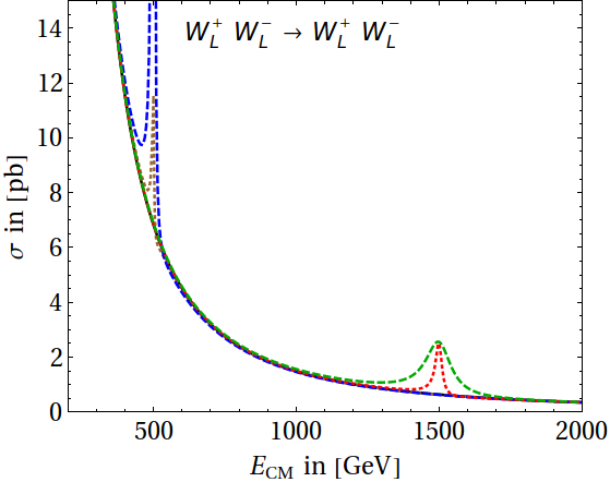
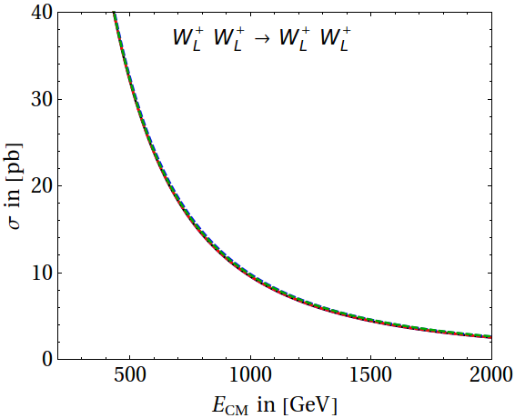
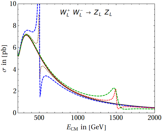
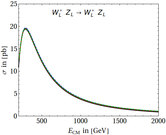
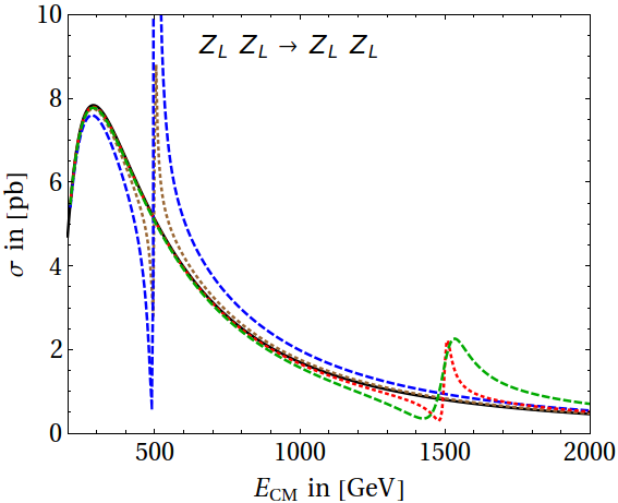
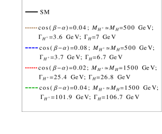
Figure 1: Plots for $VV$ scattering in 2HDM.

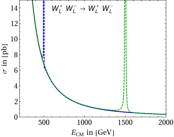
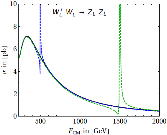
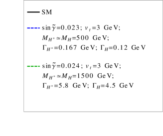
Figure 2: Plots for $VV$ scattering in Y=0 HTM.

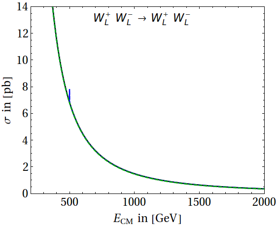
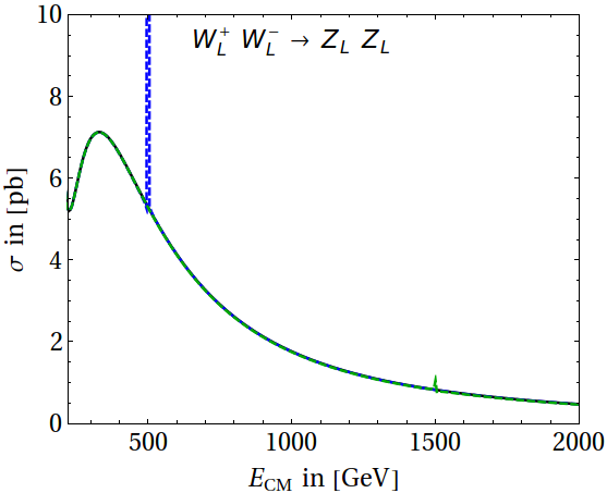
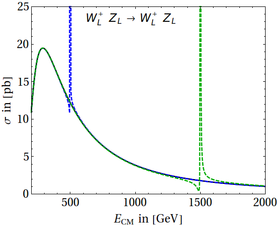
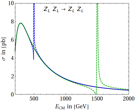
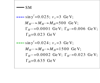
Figure 3: Plots for $VV$ scattering in Y=2 HTM.

5 Summary and conclusion

For the scattering of longitudinally polarised weak gauge bosons, we point out that the resonances arising in some extended scalar sectors can be noticed in the distribution in the subprocess centre-of-mass energies, which can play a complementary (or confirmatory) role in the search of such new scalars. Both the new physics term containing a Breit-Wigner-resonance and the interference term between the new physics and the standard model contributions involved in computing cross-sections conspire to demonstrate the effect of new scalar resonances.

We have presented our results on different scattering channels for longitudinally polarised gauge bosons in various extended scalar sectors. VBS processes are sensitive to the scalar sector as the scalars ensure the unitarity of the scattering matrix.

We worked with unapproximated polarisation vectors and used complete set of Feynman diagrams. This is the reason we have provided the complete analytical expressions which can help the reader to compute the discussed VBS processes in various extensions of the scalar sector of the standard model. Exact forms of the polarisation vectors have been used, and all relevant Feynman diagrams as well as the complete analytical expressions have been presented in the Appendix.

For the sake of illustration, we have chosen three models with an extended scalar sector, namely the 2HDM and triplet models with hypercharge $Y=0$ and $2$. All these models are endowed with heavier scalars – for the chosen benchmark points the masses are at 500 GeV or at 1500 GeV. From the presence of resonances at various VBS modes, we have tried to identify the underlying model.

The shape of the invariant mass distribution in the vicinity of the resonance is found to offer rather distinctive features in this respect. First, the decay width of the mediating scalar, occurring in the Breit-Wigner propagator, along with the other parameters of the theory, determines the small shift of the resonant point from the actual mass of the charged or neutral scalar involved. This in turn depends on the scalar VEV, and thus provides a substantial distinction between the cases where a member of an SU(2) doublet or a triplet is the mediator, because the VEV of the latter is constrained to be much smaller. In addition, the model parameters (especially the VEVs) also determine the relative contributions of the purely ‘new physics part’ and its interference term with the SM in the squared matrix element. When the former is bigger, one usually observes just a resonant peak. With sizeable or dominant contribution from the latter, a sign flip in the propagator causes a dip followed by a peak (or the other way around) in the plot against $\sqrt{s}$.

This work is aimed at pointing out the above model-specific features in longitudinal gauge boson scattering, which can supplement the phenomenology involving the scalar sector itself. A more detailed description of the collider observables that enable one to extract faithful information on the resonant peaks (or accompanying dips) will be presented in a later study.

6 Acknowledgements

The work of N.K. is supported by a fellowship from University Grants Commission, India. B.M. and A.S. acknowledge the funding available from the Department of Atomic Energy, Government of India, for the Regional Centre for Accelerator based Particle Physics (RECAPP), Harish-Chandra Research Institute. S.R. is funded by the Department of Science and Technology, India via Grant No. EMR/2014/001177. The visit of A.S. at IIT Indore was also supported from this grant. S.R. acknowledges hospitality of RECAPP while this work was in progress.

Appendix A Amplitudes for individual diagrams in the different modes of $V_{L}V_{L}$ scattering

Let $p_{1},~{}p_{2}$ are the four momenta of initial state gauge bosons and $k_{1},~{}k_{2}$ are that for the final state gauge bosons respectively.

• Let, $\epsilon(p)$ be the polarization four vector of a gauge bosons $V(\equiv W^{\pm},~{}Z$) with four momentum $p$ which satisfies the relation $\epsilon(p)\cdot p=0$. It can be written as, $\epsilon_{\mu}(p)\equiv\{\frac{|{\bf p}|}{M_{V}},\frac{E_{V}}{M_{V}}\hat{p}\}$, where $E_{V}$ is the energy of the gauge boson and is given by $E_{V}=\sqrt{|{\bf p}|^{2}+M_{V}^{2}}$. Here, $M_{V}$ is the mass of $V$. For illustrative purpose, we choose the notations as $\epsilon_{1}\equiv\epsilon(p_{1})$, $\epsilon_{2}\equiv\epsilon(p_{2})$, $\epsilon_{3}\equiv\epsilon(k_{1})$ and $\epsilon_{4}\equiv\epsilon(k_{2})$.

• Mandelstam variables are defined as: $s=(p_{1}+p_{2})^{2}$; $t=(p_{1}-k_{1})^{2}$; $u=(p_{1}-k_{2})^{2}$. In the following, $x\equiv\cos\theta$, where $\theta$ is the scattering angle.

• We use the shorthand notations $c_{W}\equiv\cos{\theta_{W}}$ and $s_{W}\equiv\sin{\theta_{W}}$, where $\theta_{W}$ is the Weinberg angle.

In the following we present the contributing Feynman diagrams and scattering amplitudes for various vector boson scattering modes in terms of total energy in the centre of momentum frame $E_{CM}\equiv\sqrt{s}$ and scattering angle. We use Unitary gauge in our calculations. Note that the coefficients $C$, $C^{\prime}$, $\hat{C}$, $\tilde{C}$ are model dependent and can be found in Appendix C.

A.1 $W_{L}^{+}(p_{1})~{}+~{}W_{L}^{-}(p_{2})\rightarrow W_{L}^{+}(k_{1})~{}+~{}W_{L}^{-}(k_{2})$

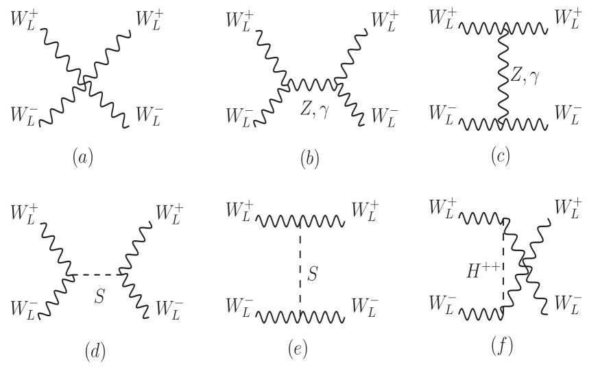
Figure 4: Generic Feynman diagrams for  $W_{L}^{+}(p_{1})~{}+~{}W_{L}^{-}(p_{2})\rightarrow W_{L}^{+}(k_{1})~{}+~{}W_{L}^{-}(k_{2})$  scattering.

$$(a) {\cal M}_{\rm p} =~{}~{}\frac{E_{CM}^{2}g_{2}^{2}}{16M_{W}^{4}}\bigg{\{}8M_{W}^{2}(1-3x)-E_{CM}^{2}\left(3-6x-x^{2}\right)\bigg{\}}.$$

$$(b) {\cal M}^{\gamma+{Z}}_{s} =~{}-\frac{g_{2}^{2}}{4M_{W}^{4}}\left(\frac{s_{W}^{2}}{s}+\frac{c_{W}^{2}}{s-M_{Z}^{2}}\right)\bigg{(}E_{CM}^{6}-12E_{CM}^{2}M_{W}^{4}-16M_{W}^{6}\bigg{)}x.$$

$$(c) {\cal M}^{\gamma+{Z}}_{t} =~{}-\frac{g_{2}^{2}}{32M_{W}^{4}}\left(\frac{s_{W}^{2}}{t}+\frac{c_{W}^{2}}{t-M_{Z}^{2}}\right)\bigg{\{}-64M_{W}^{6}(1+x)+E_{CM}^{6}(1-x)^{2}(3+x)$$

$$\hskip 56.9055pt+16E_{CM}^{2}M_{W}^{4}\left(1-7x+10x^{2}\right)-4E_{CM}^{4}M_{W}^{2}\left(3-13x+9x^{2}+x^{3}\right)\bigg{\}}.$$

$$(d) {\cal M}^{S}_{s} =~{}-\frac{(C~{}g_{2}M_{W})^{2}}{s-M_{S}^{2}}~{}\frac{\left(E_{CM}^{2}-2M_{W}^{2}\right)^{2}}{4M_{W}^{4}}.$$

$$(e) {\cal M}^{S}_{t} =~{}-\frac{(C~{}g_{2}M_{W})^{2}}{t-M_{S}^{2}}~{}\frac{\{4M_{W}^{2}+E_{CM}^{2}(1-x)\}^{2}}{16M_{W}^{4}}.$$

$$(f) {\cal M}^{H^{++}}_{u} =~{}-\frac{(\hat{C}~{}g_{2}M_{W})^{2}}{u-M^{2}_{H^{++}}}~{}\frac{\{-4M_{W}^{2}+E_{CM}^{2}(1+x)\}^{2}}{16M_{W}^{4}}.$$

A.2 $W_{L}^{+}(p_{1})~{}+~{}W_{L}^{+}(p_{2})\rightarrow W_{L}^{+}(k_{1})~{}+~{}W_{L}^{+}(k_{2})$

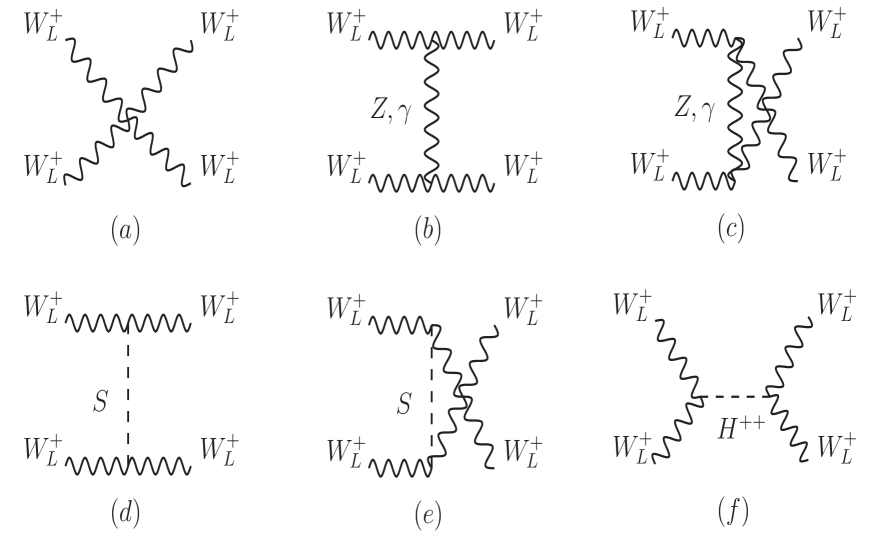
Figure 5: Generic Feynman diagrams for  $W_{L}^{+}(p_{1})~{}+~{}W_{L}^{+}(p_{2})\rightarrow W_{L}^{+}(k_{1})~{}+~{}W_{L}^{+}(k_{2})$  scattering.

$$(a) {\cal M}_{\rm p} =~{}~{}\frac{E_{CM}^{2}g_{2}^{2}c_{W}^{2}}{8M_{W}^{2}M_{Z}^{2}}\bigg{\{}4\left(M_{W}^{2}+M_{Z}^{2}\right)-E_{CM}^{2}\left(3-x^{2}\right)\bigg{\}}.$$

$$(b) {\cal M}^{W}_{t} =~{}-\frac{c_{W}^{2}g_{2}^{2}}{32M_{W}^{4}M_{Z}^{2}(t-M_{W}^{2})}\bigg{\{}3E_{CM}^{6}M_{W}^{2}-4E_{CM}^{4}M_{W}^{4}-10E_{CM}^{4}M_{W}^{2}M_{Z}^{2}$$

$$\hskip 56.9055pt+8E_{CM}^{2}M_{W}^{4}M_{Z}^{2}+2E_{CM}^{4}M_{Z}^{4}+16E_{CM}^{2}M_{W}^{2}M_{Z}^{4}-96M_{W}^{4}M_{Z}^{4}$$

$$\hskip 56.9055pt-8E_{CM}^{2}M_{Z}^{6}+32M_{W}^{2}M_{Z}^{6}+x(E_{CM}^{4}M_{W}^{2}\text{ }x^{2}-5E_{CM}^{4}M_{W}^{2}$$

$$\hskip 56.9055pt+12E_{CM}^{2}M_{W}^{4}+24E_{CM}^{2}M_{W}^{2}M_{Z}^{2}+16M_{W}^{4}M_{Z}^{2}$$

$$\hskip 56.9055pt-4E_{CM}^{2}M_{Z}^{4})\sqrt{(E_{CM}^{2}-4M_{W}^{2})(E_{CM}^{2}-4M_{Z}^{2})}+E_{CM}^{6}M_{W}^{2}x^{2}$$

$$\hskip 56.9055pt-16E_{CM}^{4}M_{W}^{4}x^{2}+32E_{CM}^{2}M_{W}^{6}x^{2}-22E_{CM}^{4}M_{W}^{2}M_{Z}^{2}x^{2}$$

$$\hskip 56.9055pt+96E_{CM}^{2}M_{W}^{4}M_{Z}^{2}x^{2}+2E_{CM}^{4}M_{Z}^{4}x^{2}+32E_{CM}^{2}M_{W}^{2}M_{Z}^{4}x^{2}\bigg{\}}.$$

$$(c) {\cal M}^{W}_{u} =~{}-\frac{c_{W}^{2}g_{2}^{2}}{32M_{W}^{4}M_{Z}^{2}(u-M_{W}^{2})}\bigg{\{}3E_{CM}^{6}M_{W}^{2}-4E_{CM}^{4}M_{W}^{4}-10E_{CM}^{4}M_{W}^{2}M_{Z}^{2}$$

$$\hskip 56.9055pt+8E_{CM}^{2}M_{W}^{4}M_{Z}^{2}+2E_{CM}^{4}M_{Z}^{4}+16E_{CM}^{2}M_{W}^{2}M_{Z}^{4}-96M_{W}^{4}M_{Z}^{4}$$

$$\hskip 56.9055pt-8E_{CM}^{2}M_{Z}^{6}+32M_{W}^{2}M_{Z}^{6}-x(E_{CM}^{4}M_{W}^{2}\text{ }x^{2}-5E_{CM}^{4}M_{W}^{2}$$

$$\hskip 56.9055pt+12E_{CM}^{2}M_{W}^{4}+24E_{CM}^{2}M_{W}^{2}M_{Z}^{2}+16M_{W}^{4}M_{Z}^{2}$$

$$\hskip 56.9055pt-4E_{CM}^{2}M_{Z}^{4})\sqrt{(E_{CM}^{2}-4M_{W}^{2})(E_{CM}^{2}-4M_{Z}^{2})}+E_{CM}^{6}M_{W}^{2}x^{2}$$

$$\hskip 56.9055pt-16E_{CM}^{4}M_{W}^{4}x^{2}+32E_{CM}^{2}M_{W}^{6}x^{2}-22E_{CM}^{4}M_{W}^{2}M_{Z}^{2}x^{2}$$

$$\hskip 56.9055pt+96E_{CM}^{2}M_{W}^{4}M_{Z}^{2}x^{2}+2E_{CM}^{4}M_{Z}^{4}x^{2}+32E_{CM}^{2}M_{W}^{2}M_{Z}^{4}x^{2}\bigg{\}}.$$

$$(d) {\cal M}^{S}_{s} =~{}-\frac{(C~{}g_{2}M_{W})(C^{\prime}~{}\frac{g_{2}M_{Z}}{c_{W}})}{s-M_{S}^{2}}~{}\frac{\left(E_{CM}^{2}-2M_{W}^{2}\right)\left(E_{CM}^{2}-2M_{Z}^{2}\right)}{4M_{W}^{2}M_{Z}^{2}}.$$

$$(e) {\cal M}^{H^{+}}_{t} =~{}-\frac{(\widetilde{C}~{}\frac{g_{2}M_{Z}}{c_{W}})^{2}}{t-M_{H^{+}}^{2}}~{}\frac{\big{\{}\sqrt{\left(E_{CM}^{2}-4M_{W}^{2}\right)\left(E_{CM}^{2}-4M_{Z}^{2}\right)}-E_{CM}^{2}x\big{\}}^{2}}{16M_{W}^{2}M_{Z}^{2}}.$$

$$(f) {\cal M}^{H^{+}}_{u} =~{}-\frac{(\widetilde{C}~{}\frac{g_{2}M_{Z}}{c_{W}})^{2}}{u-M_{H^{+}}^{2}}~{}\frac{\big{\{}\sqrt{\left(E_{CM}^{2}-4M_{W}^{2}\right)\left(E_{CM}^{2}-4M_{Z}^{2}\right)}+E_{CM}^{2}x\big{\}}^{2}}{16M_{W}^{2}M_{Z}^{2}}.$$

A.3 $W_{L}^{+}(p_{1})~{}+~{}W_{L}^{-}(p_{2})\rightarrow Z_{L}(k_{1})~{}+~{}Z_{L}(k_{2})$

Figure 6: Generic Feynman diagrams for  $W_{L}^{+}(p_{1})~{}+~{}W_{L}^{-}(p_{2})\rightarrow Z_{L}(k_{1})~{}+~{}Z_{L}(k_{2})$  scattering.

$$(a) {\cal M}_{\rm p} =~{}\frac{E_{CM}^{2}g_{2}^{2}c_{W}^{2}}{8M_{W}^{2}M_{Z}^{2}}\bigg{\{}4\left(M_{W}^{2}+M_{Z}^{2}\right)-E_{CM}^{2}\left(3-x^{2}\right)\bigg{\}}.$$

$$(b) {\cal M}^{W}_{t} =~{}-\frac{c_{W}^{2}g_{2}^{2}}{32M_{W}^{4}M_{Z}^{2}(t-M_{W}^{2})}\bigg{\{}3E_{CM}^{6}M_{W}^{2}-4E_{CM}^{4}M_{W}^{4}-10E_{CM}^{4}M_{W}^{2}M_{Z}^{2}$$

$$\hskip 56.9055pt+8E_{CM}^{2}M_{W}^{4}M_{Z}^{2}+2E_{CM}^{4}M_{Z}^{4}+16E_{CM}^{2}M_{W}^{2}M_{Z}^{4}-96M_{W}^{4}M_{Z}^{4}-8E_{CM}^{2}M_{Z}^{6}$$

$$\hskip 56.9055pt+32M_{W}^{2}M_{Z}^{6}+x(E_{CM}^{4}M_{W}^{2}\text{ }x^{2}-5E_{CM}^{4}M_{W}^{2}+12E_{CM}^{2}M_{W}^{4}-4E_{CM}^{2}M_{Z}^{4}$$

$$\hskip 56.9055pt+16M_{W}^{4}M_{Z}^{2}+24E_{CM}^{2}M_{W}^{2}M_{Z}^{2})\sqrt{(E_{CM}^{2}-4M_{W}^{2})(E_{CM}^{2}-4M_{Z}^{2})}$$

$$\hskip 56.9055pt+E_{CM}^{6}M_{W}^{2}x^{2}-16E_{CM}^{4}M_{W}^{4}x^{2}+32E_{CM}^{2}M_{W}^{6}x^{2}-22E_{CM}^{4}M_{W}^{2}M_{Z}^{2}x^{2}$$

$$\hskip 56.9055pt+96E_{CM}^{2}M_{W}^{4}M_{Z}^{2}x^{2}+2E_{CM}^{4}M_{Z}^{4}x^{2}+32E_{CM}^{2}M_{W}^{2}M_{Z}^{4}x^{2}\bigg{\}}.$$

$$(c) {\cal M}^{W}_{u} =~{}-\frac{c_{W}^{2}g_{2}^{2}}{32M_{W}^{4}M_{Z}^{2}(u-M_{W}^{2})}\bigg{\{}3E_{CM}^{6}M_{W}^{2}-4E_{CM}^{4}M_{W}^{4}-10E_{CM}^{4}M_{W}^{2}M_{Z}^{2}$$

$$\hskip 56.9055pt+8E_{CM}^{2}M_{W}^{4}M_{Z}^{2}+2E_{CM}^{4}M_{Z}^{4}+16E_{CM}^{2}M_{W}^{2}M_{Z}^{4}-96M_{W}^{4}M_{Z}^{4}-8E_{CM}^{2}M_{Z}^{6}$$

$$\hskip 56.9055pt+32M_{W}^{2}M_{Z}^{6}-x(E_{CM}^{4}M_{W}^{2}\text{ }x^{2}-5E_{CM}^{4}M_{W}^{2}+12E_{CM}^{2}M_{W}^{4}-4E_{CM}^{2}M_{Z}^{4}$$

$$\hskip 56.9055pt+16M_{W}^{4}M_{Z}^{2}+24E_{CM}^{2}M_{W}^{2}M_{Z}^{2})\sqrt{(E_{CM}^{2}-4M_{W}^{2})(E_{CM}^{2}-4M_{Z}^{2})}$$

$$\hskip 56.9055pt+E_{CM}^{6}M_{W}^{2}x^{2}-16E_{CM}^{4}M_{W}^{4}x^{2}+32E_{CM}^{2}M_{W}^{6}x^{2}-22E_{CM}^{4}M_{W}^{2}M_{Z}^{2}x^{2}$$

$$\hskip 56.9055pt+96E_{CM}^{2}M_{W}^{4}M_{Z}^{2}x^{2}+2E_{CM}^{4}M_{Z}^{4}x^{2}+32E_{CM}^{2}M_{W}^{2}M_{Z}^{4}x^{2}\bigg{\}}.$$

$$(d) {\cal M}^{S}_{s} =~{}-\frac{(C~{}g_{2}M_{W})(C^{\prime}~{}\frac{g_{2}M_{Z}}{c_{W}})}{s-M_{S}^{2}}~{}\frac{\left(E_{CM}^{2}-2M_{W}^{2}\right)\left(E_{CM}^{2}-2M_{Z}^{2}\right)}{4M_{W}^{2}M_{Z}^{2}}.$$

$$(e) {\cal M}^{H^{+}}_{t} =~{}-\frac{(\widetilde{C}~{}\frac{g_{2}M_{Z}}{c_{W}})^{2}}{t-M_{H^{+}}^{2}}~{}\frac{\big{\{}\sqrt{\left(E_{CM}^{2}-4M_{W}^{2}\right)\left(E_{CM}^{2}-4M_{Z}^{2}\right)}-E_{CM}^{2}x\big{\}}^{2}}{16M_{W}^{2}M_{Z}^{2}}.$$

$$(f) {\cal M}^{H^{+}}_{u} =~{}-\frac{(\widetilde{C}~{}\frac{g_{2}M_{Z}}{c_{W}})^{2}}{u-M_{H^{+}}^{2}}~{}\frac{\big{\{}\sqrt{\left(E_{CM}^{2}-4M_{W}^{2}\right)\left(E_{CM}^{2}-4M_{Z}^{2}\right)}+E_{CM}^{2}x\big{\}}^{2}}{16M_{W}^{2}M_{Z}^{2}}.$$

A.4 $W_{L}^{+}(p_{1})~{}+~{}Z_{L}(p_{2})\rightarrow W_{L}^{+}(k_{1})~{}+~{}Z_{L}(k_{2})$

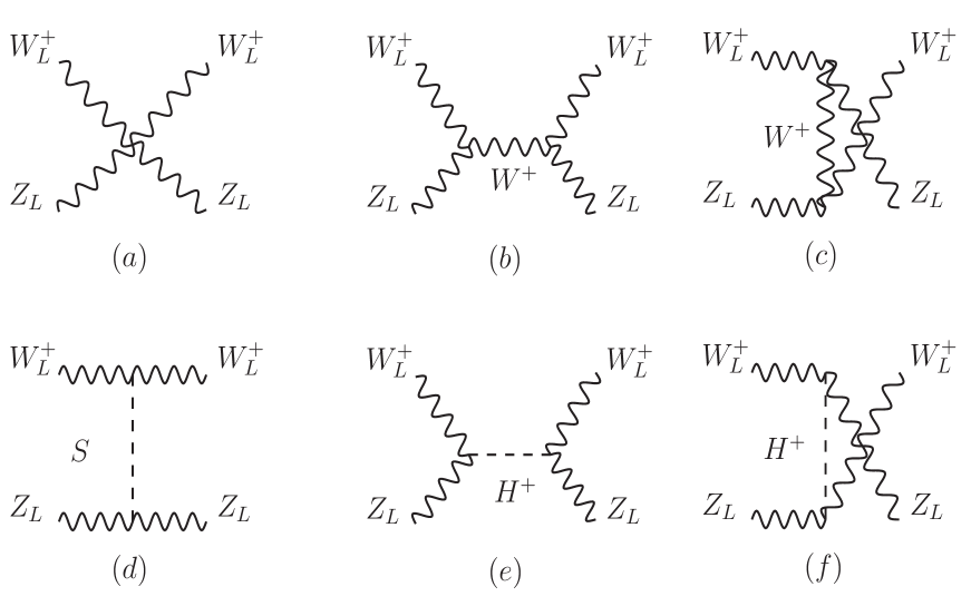
Figure 7: Generic Feynman diagrams for  $W_{L}^{+}(p_{1})~{}+~{}Z_{L}(p_{2})\rightarrow W_{L}^{+}(k_{1})~{}+~{}Z_{L}(k_{2})$  scattering.

$$(a) {\cal M}_{\rm p} =~{}-\frac{c_{W}^{2}g^{2}}{16E_{CM}^{4}M_{W}^{2}M_{Z}^{2}}\bigg{\{}4E_{CM}^{2}\left(M_{W}^{2}-M_{Z}^{2}\right)^{2}\left(M_{W}^{2}+M_{Z}^{2}\right)(x-1)$$

$$\hskip 56.9055pt+\left(M_{W}^{2}-M_{Z}^{2}\right)^{4}(1-x)^{2}+2E_{CM}^{4}\left(M_{W}^{2}-M_{Z}^{2}\right)^{2}\left(1-4x-x^{2}\right)$$

$$\hskip 56.9055pt+4E_{CM}^{6}\left(M_{W}^{2}+M_{Z}^{2}\right)(1+3x)-E_{CM}^{8}\left(3+6x-x^{2}\right)\bigg{\}}.$$

$$(b) {\cal M}^{W}_{s} =~{}-\frac{c_{W}^{2}g^{2}}{4E_{CM}^{2}M_{W}^{4}M_{Z}^{2}(s-M_{W}^{2})}\bigg{[}E_{CM}^{6}\left(M_{W}^{2}-M_{Z}^{2}\right)^{2}-\left(M_{W}^{5}-M_{W}M_{Z}^{4}\right)^{2}(1-x)$$

$$\hskip 56.9055pt+E_{CM}^{8}M_{W}^{2}x-E_{CM}^{4}\big{\{}2M_{Z}^{6}-4M_{W}^{4}M_{Z}^{2}(1-2x)-M_{W}^{2}M_{Z}^{4}(1-2x)$$

$$\hskip 56.9055pt+M_{W}^{6}(3+2x)\big{\}}+E_{CM}^{2}\big{\{}M_{W}^{2}+M_{Z}^{2})(3M_{W}^{6}+M_{W}^{2}M_{Z}^{4}+M_{Z}^{6}$$

$$\hskip 56.9055pt-M_{W}^{4}M_{Z}^{2}(5+8x)\big{\}}\bigg{]}.$$

$$(c) {\cal M}^{W}_{u} =~{}~{}\frac{M_{Z}^{2}c_{W}^{2}g^{2}}{32E_{CM}^{6}M_{W}^{4}(u-M_{W}^{2})}\bigg{[}\big{\{}M_{W}^{2}(M_{W}^{2}-M_{Z}^{2})^{6}(x-1)^{3}+E_{CM}^{12}M_{W}^{2}(-3+x)(1+x)^{2}$$

$$\hskip 56.9055pt-2E_{CM}^{2}(M_{W}^{2}-M_{Z}^{2})^{4}(1-x)^{2}(-M_{Z}^{4}+M_{W}^{4}x+M_{W}^{2}M_{Z}^{2}(3+x)\big{\}}$$

$$\hskip 56.9055pt+2E_{CM}^{10}\big{\{}M_{Z}^{4}(1+x)^{2}+M_{W}^{2}M_{Z}^{2}(1+9x+7x^{2}-x^{3})$$

$$\hskip 56.9055pt+M_{W}^{4}(4+15x+10x^{2}-x^{3})\big{\}}+4E_{CM}^{6}\big{\{}M_{Z}^{8}(3-x^{2})$$

$$\hskip 56.9055pt+M_{W}^{6}M_{Z}^{2}(9-9x-7x^{2}-x^{3})-M_{W}^{8}(2-x-10x^{2}-x^{3})$$

$$\hskip 56.9055pt-M_{W}^{2}M_{Z}^{6}(9-x-15x^{2}-x^{3})+M_{W}^{4}M_{Z}^{4}(15-9x-17x^{2}-x^{3})\big{\}}$$

$$\hskip 56.9055pt-E_{CM}^{4}(M_{W}^{2}-M_{Z}^{2})^{2}\big{\{}8M_{Z}^{6}(1-x)-M_{W}^{6}(7+5x-11x^{2}-x^{3})$$

$$\hskip 56.9055pt-M_{W}^{2}M_{Z}^{4}(23-11x-11x^{2}-x^{3})+2M_{W}^{4}M_{Z}^{2}(3+25x-27x^{2}-x^{3})\big{\}}$$

$$\hskip 56.9055pt-E_{CM}^{8}\big{\{}8M_{Z}^{6}(1+x)+2M_{W}^{4}M_{Z}^{2}(9+25x+31x^{2}-x^{3})$$

$$\hskip 56.9055pt-M_{W}^{2}M_{Z}^{4}(13-19x-49x^{2}-x^{3})+M_{W}^{6}(3+35x+49x^{2}+x^{3})\big{\}}\bigg{]}.$$

$$(d) {\cal M}^{S}_{t} =~{}-\frac{(C~{}g_{2}M_{W})(C^{\prime}~{}\frac{g_{2}M_{Z}}{c_{W}})}{t-M_{S}^{2}}~{}\bigg{(}\frac{1}{16E_{CM}^{4}M_{W}^{2}M_{Z}^{2}}\bigg{)}~{}\bigg{[}\big{\{}(x-1)\big{(}E_{CM}^{4}+(M_{W}^{2}-M_{Z}^{2})^{2}\big{)}$$

$$\hskip 56.9055pt+2E_{CM}^{2}\big{(}M_{Z}^{2}(1-x)+M_{W}^{2}(1+x)\big{)}\big{\}}\big{\{}(x-1)\big{(}E_{CM}^{4}+(M_{W}^{2}-M_{Z}^{2})^{2}\big{)}$$

$$\hskip 56.9055pt+2E_{CM}^{2}\big{(}M_{W}^{2}(1-x)-M_{Z}^{2}(1+x)\big{)}\big{\}}\bigg{]}.$$

$$(e) {\cal M}^{H^{+}}_{u} =~{}-\frac{(\widetilde{C}~{}\frac{g_{2}M_{Z}}{c_{W}})^{2}}{u-M_{H^{+}}^{2}}~{}\bigg{(}\frac{1}{16E_{CM}^{4}M_{W}^{2}M_{Z}^{2}}\bigg{)}\bigg{\{}2E_{CM}^{2}(M_{W}^{2}+M_{Z}^{2})-(M_{W}^{2}-M_{Z}^{2})^{2}(1-x)$$

$$\hskip 284.52756pt-E_{CM}^{4}(1+x)\bigg{\}}^{2}.$$

$$(f) {\cal M}^{H^{+}}_{s} =~{}~{}-\frac{(\widetilde{C}~{}\frac{g_{2}M_{Z}}{c_{W}})^{2}}{s-M_{H^{+}}^{2}}~{}\frac{(-E_{CM}^{2}+M_{W}^{2}+M_{Z}^{2})^{2}}{4M_{W}^{2}M_{Z}^{2}}.$$

A.5 $Z_{L}(p_{1})~{}+~{}Z_{L}(p_{2})\rightarrow Z_{L}(k_{1})~{}+~{}Z_{L}(k_{2})$

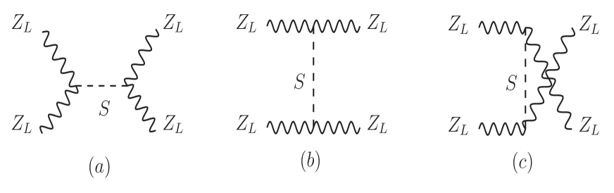
Figure 8: Generic Feynman diagrams for  $Z_{L}(p_{1})~{}+~{}Z_{L}(p_{2})\rightarrow Z_{L}(k_{1})~{}+~{}Z_{L}(k_{2})$  scattering.

$$(a) {\cal M}^{S}_{s} =~{}~{}-\frac{(C^{\prime}~{}\frac{g_{2}M_{Z}}{c_{W}})^{2}}{(s-M_{S}^{2})}~{}\frac{(E_{CM}^{2}-2M_{Z}^{2})^{2}}{4M_{Z}^{4}}.$$

$$(b) {\cal M}^{S}_{t} =~{}~{}-\frac{(C^{\prime}~{}\frac{g_{2}M_{Z}}{c_{W}})^{2}}{(t-M_{S}^{2})}~{}\frac{\big{\{}4M_{Z}^{2}+E_{CM}^{2}(-1+x)\big{\}}^{2}}{16M_{Z}^{4}}.$$

$$(c) {\cal M}^{S}_{u} =~{}~{}-\frac{(C^{\prime}~{}\frac{g_{2}M_{Z}}{c_{W}})^{2}}{(u-M_{S}^{2})}~{}\frac{\big{\{}-4M_{Z}^{2}+E_{CM}^{2}(1+x)\big{\}}^{2}}{16M_{Z}^{4}}.$$

Appendix B Total amplitude for the different modes of $V_{L}V_{L}$ scattering

Generally when $E_{CM}\gg M_{i}$ ($i\equiv W,Z,h,H,H^{\pm},H^{\pm\pm}$), one can express $V_{L}V_{L}\rightarrow V_{L}V_{L}$ scattering amplitude as,

$${\cal M} = A_{4}~{}E_{CM}^{4}+A_{2}~{}E_{CM}^{2}+A_{0}+A_{-2}~{}E_{CM}^{-2}+....$$ (B-1)

The coefficient of $E_{CM}^{4}$ term i.e., $A_{4}$ is always zero from gauge symmetry. $A_{2}$ also vanishes after scalar sector contributions are added to the gauge contributions, thus ensuring unitarity of the scattering matrix. The energy independent part $A_{0}$ becomes the dominant one at high energy. It is given by

$$A_{0} = A_{0,V}+A_{0,S}\,,$$ (B-2)

where $A_{0,V}$ and $A_{0,S}$ are contributions from the gauge bosons and the scalars respectively. To enable the reader to readily evaluate extended scalar sector contributions to VBS processes we will now present expressions for $A_{0,V}$ and $A_{0,S}$ in various vector bosons scattering modes.

• $W_{L}^{+}W_{L}^{-}\rightarrow W_{L}^{+}W_{L}^{-}$

  $$A_{0,V} = -\frac{g_{2}^{2}}{4M_{W}^{4}(1-x)}\bigg{\{}-c_{W}^{2}M_{Z}^{4}(3+x^{2})+2c_{W}^{2}M_{W}^{2}M_{Z}^{2}(3+6x-x^{2})$$

  $$\hskip 213.39566pt-4M_{W}^{4}(1+4x-x^{2})\bigg{\}},$$

  $$A_{0,S} = -\frac{1}{4M_{W}^{4}}\bigg{\{}\big{(}{g_{2}M_{W}}\hat{C}\big{)}^{2}\big{(}M_{H^{++}}^{2}+2M_{W}^{2}(1-x)\big{)}$$

  $$\hskip 108.12054pt+2\sum_{S=h,H}\big{(}g_{2}{M_{W}}C\big{)}^{2}\big{(}{M_{S}}^{2}-M_{W}^{2}(1-x)\big{)}\bigg{\}}.$$

• $W_{L}^{+}W_{L}^{+}\rightarrow W_{L}^{+}W_{L}^{+}$

  $$A_{0,V} = -\frac{{g_{2}}^{2}}{2M_{W}^{4}(1-x^{2})}\bigg{\{}c_{W}^{2}M_{Z}^{4}(3+x^{2})+4M_{W}^{4}(1+3x^{2})-2c_{W}^{2}M_{W}^{2}M_{Z}^{2}(3+5x^{2})\bigg{\}},$$

  $$A_{0,S} = -\frac{1}{4M_{W}^{4}}\bigg{\{}({g_{2}M_{W}}\hat{C})^{2}(M_{H^{++}}^{2}-4M_{W}^{2})+2\sum_{S=h,H}(g_{2}{M_{W}}C)^{2}(M_{S}^{2}+2M_{W}^{2})\bigg{\}}.$$

• $W_{L}^{+}W_{L}^{-}\rightarrow Z_{L}Z_{L}$

  $$A_{0,V} = \frac{c_{W}^{2}g_{2}^{2}M_{Z}^{2}}{2M_{W}^{4}(1-x^{2})}\bigg{\{}-M_{Z}^{2}(1-x^{2})+2M_{W}^{2}(1+x^{2})\bigg{\}},$$

  $$A_{0,S} = \frac{1}{4M_{W}^{2}M_{Z}^{2}}\bigg{\{}-2\bigg{(}\frac{g_{2}M_{Z}}{c_{W}}\widetilde{C}\bigg{)}^{2}\big{(}M_{H^{+}}^{2}+M_{W}^{2}+M_{Z}^{2}\big{)}$$

  $$\hskip 56.9055pt+\sum_{S=h,H}\bigg{(}\frac{g_{2}M_{Z}}{c_{W}}C^{\prime}\bigg{)}\big{(}g_{2}M_{W}C\big{)}\big{(}-{M_{S}}^{2}+2(M_{W}^{2}+M_{Z}^{2})\big{)}\bigg{\}}.$$

• $W_{L}^{+}Z_{L}\rightarrow W_{L}^{+}Z_{L}$

  $$A_{0,V} = \frac{c_{W}^{2}{g_{2}}^{2}M_{Z}^{2}}{4M_{W}^{4}(1+x)}\bigg{\{}-2M_{W}^{2}(1-x)+M_{Z}^{2}(1+x)^{2}\bigg{\}},$$

  $$A_{0,S} = -\frac{1}{4M_{W}^{2}M_{Z}^{2}}\bigg{\{}\bigg{(}\frac{g_{2}M_{Z}}{c_{W}}\widetilde{C}\bigg{)}^{2}\big{(}2M_{H^{+}}^{2}-(M_{W}^{2}+M_{Z}^{2})(1+x)\big{)}$$

  $$\hskip 56.9055pt+\sum_{S=h,H}\bigg{(}\frac{g_{2}M_{Z}}{c_{W}}C^{\prime}\bigg{)}\big{(}g_{2}M_{W}C\big{)}\big{(}M_{S}^{2}+(M_{W}^{2}+M_{Z}^{2})(1+x)\big{)}\bigg{\}}.$$

• $Z_{L}Z_{L}\rightarrow Z_{L}Z_{L}$

  $$A_{0,V} = 0,$$

  $$A_{0,S} = -\frac{3}{4M_{Z}^{4}}\sum_{S=h,H}\bigg{(}\frac{g_{2}M_{Z}}{c_{W}}C^{\prime}\bigg{)}^{2}M_{S}^{2}.$$

Appendix C Required Feynman rules for vector boson scattering

The Feynman rules for the different vertices with the assumption that all momenta and fields are incoming.

$\displaystyle:ig_{2}^{2}(2g^{\mu\lambda}g^{\sigma\nu}-g^{\mu\sigma}g^{\nu\lambda}-g^{\sigma\lambda}g^{\mu\nu}).$

(C-1)

$\displaystyle:-ig_{2}^{2}c_{W}^{2}(2g^{\mu\nu}g^{\sigma\lambda}-g^{\nu\sigma}g^{\mu\lambda}-g^{\nu\lambda}g^{\mu\sigma}).$

(C-2)

$\displaystyle:ig_{2}c_{W}\{(p-q)^{\lambda}~{}g^{\mu\nu}+(q-k)^{\mu}~{}g^{\lambda\nu}+(k-p)^{\nu}~{}g^{\mu\lambda}\}.$

(C-3)

$\displaystyle:ig_{2}s_{W}\{(p-q)^{\lambda}~{}g^{\mu\nu}+(q-k)^{\mu}~{}g^{\lambda\nu}+(k-p)^{\nu}~{}g^{\mu\lambda}\}.$

(C-4)

$\displaystyle:{ig_{2}}{M_{W}}g_{\mu\nu}C$, where $C$ is given by:

$${\rm SM} :\left\{\begin{array}[]{l}{\rm for}~{}~{}h,~{}~{}C=1,\\ {\rm for}~{}~{}H,~{}~{}C=0,\end{array}\right.$$ (C-5)

$${\rm 2HDM} :\left\{\begin{array}[]{l}{\rm for}~{}~{}h,~{}~{}C=\sin(\beta-\alpha),\\ {\rm for}~{}~{}H,~{}~{}C=\cos(\beta-\alpha),\end{array}\right.$$

$${\rm Y=0~{}~{}HTM} :\left\{\begin{array}[]{l}{\rm for}~{}~{}h,~{}~{}C=(\cos\widetilde{\beta}\cos{\widetilde{\gamma}}+2\sin\widetilde{\beta}\sin{\widetilde{\gamma}}),\\ {\rm for}~{}~{}H,~{}~{}C=(-\cos\widetilde{\beta}\sin{\widetilde{\gamma}}+2\sin\widetilde{\beta}\cos{\widetilde{\gamma}}),\end{array}\right.$$

$${\rm Y=2~{}~{}HTM} :\left\{\begin{array}[]{l}{\rm for}~{}~{}h,~{}~{}C=(\cos{\beta^{\prime}}\cos{\gamma^{\prime}}+\sqrt{2}\sin{\beta^{\prime}}\sin{\gamma^{\prime}}),\\ {\rm for}~{}~{}H,~{}~{}C=(-\cos{\beta^{\prime}}\sin{\gamma^{\prime}}+\sqrt{2}\sin{\beta^{\prime}}\cos{\gamma^{\prime}}).\end{array}\right.$$

$\displaystyle:\frac{ig_{2}M_{Z}}{c_{W}}g_{\mu\nu}C^{\prime}$, where $C^{\prime}$ is given by:

$${\rm SM} : \left\{\begin{array}[]{l}{\rm for}~{}~{}h,~{}~{}C^{\prime}=1,\\ {\rm for}~{}~{}H,~{}~{}C^{\prime}=0,\end{array}\right.$$ (C-6)

$${\rm 2HDM} : \left\{\begin{array}[]{l}{\rm for}~{}~{}h,~{}~{}C^{\prime}=\sin(\beta-\alpha),\\ {\rm for}~{}~{}H,~{}~{}C^{\prime}=\cos(\beta-\alpha),\end{array}\right.$$

$${\rm Y=0~{}~{}HTM} : \left\{\begin{array}[]{l}{\rm for}~{}~{}h,~{}~{}C^{\prime}=\cos\widetilde{\gamma},\\ {\rm for}~{}~{}H,~{}~{}C^{\prime}=-\sin{\widetilde{\gamma}},\end{array}\right.$$

$${\rm Y=2~{}~{}HTM} : \left\{\begin{array}[]{l}{\rm for}~{}~{}h,~{}~{}C^{\prime}=(\cos{\delta^{\prime}}\cos{\gamma^{\prime}}+2\sin{\delta^{\prime}}\sin{\gamma^{\prime}}),\\ {\rm for}~{}~{}H,~{}~{}C^{\prime}=(-\cos{\delta^{\prime}}\sin{\gamma^{\prime}}+2\sin{\delta^{\prime}}\cos{\gamma^{\prime}}).\end{array}\right.$$

$\displaystyle~{}~{}~{}:\frac{ig_{2}M_{Z}}{c_{W}}g_{\mu\nu}\widetilde{C}$, where $\widetilde{C}$ is given by:

$${\rm SM}:\hskip 85.35826pt\widetilde{C}=0,$$ (C-7)

$${\rm 2HDM}:\hskip 68.28644pt\widetilde{C}=0,$$

$$Y=0{\rm~{}~{}HTM}:\hskip 36.98866pt\widetilde{C}=\sin\widetilde{\beta}\cos\widetilde{\beta}~{}\frac{M_{W}}{M_{Z}},$$

$$Y=2{\rm~{}~{}HTM}:\hskip 36.98866pt\widetilde{C}=c_{W}\bigg{\{}\sin{\beta^{\prime}}\cos{\delta^{\prime}}s_{W}^{2}-\frac{(1+s_{W}^{2})}{\sqrt{2}}\cos{\beta^{\prime}}\sin{\delta^{\prime}}\bigg{\}}.$$

$\displaystyle~{}~{}~{}:{ig_{2}M_{W}}g_{\mu\nu}\hat{C}$, where $\hat{C}$ is given by:

$${\rm SM}:\hskip 85.35826pt\hat{C}=0,$$ (C-8)

$${\rm 2HDM}:\hskip 68.28644pt\hat{C}=0,$$

$$Y=0{\rm~{}~{}HTM}:\hskip 36.98866pt\hat{C}=0,$$

$$Y=2{\rm~{}~{}HTM}:\hskip 36.98866pt\hat{C}=2\sin{\beta^{\prime}}.\qquad\qquad\qquad\qquad\qquad\qquad~{}~{}~{}~{}~{}$$

References

• [1] G. Aad et al. [ATLAS Collaboration], Phys. Lett. B 716, 1 (2012) [arXiv:1207.7214 [hep-ex]].
• [2] S. Chatrchyan et al. [CMS Collaboration], Phys. Lett. B 716, 30 (2012) [arXiv:1207.7235 [hep-ex]].
• [3] N. G. Deshpande and E. Ma, Phys. Rev. D 18, 2574 (1978). For a review, see for example, N. Khan and S. Rakshit, Phys. Rev. D 92, 055006 (2015) [arXiv:1503.03085 [hep-ph]].
• [4] S. Dawson, hep-ph/9901280.
• [5] G. Bhattacharyya, D. Das and P. B. Pal, Phys. Rev. D 87, 011702 (2013) [arXiv:1212.4651 [hep-ph]].
• [6] D. Choudhury, R. Islam and A. Kundu, Phys. Rev. D 88, 013014 (2013) [arXiv:1212.4652 [hep-ph]].
• [7] J. Chang, K. Cheung, C. T. Lu and T. C. Yuan, Phys. Rev. D 87, 093005 (2013) [arXiv:1303.6335 [hep-ph]].
• [8] K. Cheung, C. W. Chiang and T. C. Yuan, Phys. Rev. D 78, 051701 (2008) [arXiv:0803.2661 [hep-ph]].
• [9] B. W. Lee, C. Quigg and H. B. Thacker, Phys. Rev. D 16, 1519 (1977).
• [10] G. C. Branco, P. M. Ferreira, L. Lavoura, M. N. Rebelo, M. Sher and J. P. Silva, Phys. Rept.  516, 1 (2012) [arXiv:1106.0034 [hep-ph]].
• [11] N. Chakrabarty, U. K. Dey and B. Mukhopadhyaya, JHEP 1412, 166 (2014) [arXiv:1407.2145 [hep-ph]].
• [12] A. Pich and P. Tuzon, Phys. Rev. D 80, 091702 (2009) [arXiv:0908.1554 [hep-ph]].
• [13] G. Aad et al. [ATLAS Collaboration], Eur. Phys. J. C 76, no. 1, 6 (2016) [arXiv:1507.04548 [hep-ex]]; V. Khachatryan et al. [CMS Collaboration], Eur. Phys. J. C 75, 212 (2015) [arXiv:1412.8662 [hep-ex]].
• [14] M. C. Chen, S. Dawson and C. B. Jackson, Phys. Rev. D 78, 093001 (2008) [arXiv:0809.4185 [hep-ph]].
• [15] J. R. Forshaw, A. Sabio Vera and B. E. White, JHEP 0306, 059 (2003) [hep-ph/0302256].
• [16] J. R. Forshaw, D. A. Ross and B. E. White, JHEP 0110, 007 (2001) [hep-ph/0107232].
• [17] A. Arhrib, R. Benbrik, M. Chabab, G. Moultaka, M. C. Peyranere, L. Rahili and J. Ramadan, Phys. Rev. D 84, 095005, (2011) [arXiv:1105.1925 [hep-ph]].
• [18] A. Broggio, E. J. Chun, M. Passera, K. M. Patel and S. K. Vempati, JHEP 1411, 058 (2014) [arXiv:1409.3199 [hep-ph]].
• [19] D. Das and I. Saha, Phys. Rev. D 91, no. 9, 095024 (2015) [arXiv:1503.02135 [hep-ph]].