Concepts of polymer statistical topology

Abstract

I review few conceptual steps in analytic description of topological interactions, which constitute the basis of a new interdisciplinary branch in mathematical physics, emerged at the edge of topology and statistical physics of fluctuating non-phantom rope-like objects. This new branch is called statistical (or probabilistic) topology.

I Introduction: What we are talking about?

How to peel an orange, without removing its skin? Can one make an omelet from unbroken eggs? Can one smoothly (without tops) comb hairy billiard ball (the sphere), or a donut (the torus)? Why one cannot tie a knot on a telegraph wire, stretched along the railway line? These and similar, often entertaining and seemingly naive questions are directly related to the topology. I will be interested in a rather narrow range of problems associated with so-called low-dimensional topology, i.e., with the topology of systems containing long linear hurly-burly threads of different physical nature. As these objects, one can play with polymeric chains, vortex lines in superconductors, strings in quantum field theory, etc.

It is worth noting that the low-dimensional topology is a pretty insidious, or, better to say ”serpentine” science, because the daily use of ropes and wires, being trivial for ”kitchen tasks”, becomes almost useless for mathematical description of knots. Careful tying shoe laces does not help much in constructing topological invariants, determination of physical and geometric properties of highly entangled polymeric networks, folded proteins, DNAs in chromosomes, etc. Moreover, even obvious notions form the everyday’s experience seem to be incorrect: for example, any child knows what the knotted rope is, and what is its difference from the unknotted one, however, this knowledge fails being translated into mathematically rigorous terms: one cannot define a knot on any open curve, and to talk seriously about knots, only closed paths should be dealt with. Indeed, having free ends of the thread, one can always transform any two arbitrary conformations of threads into each other by a continuous deformation. Therefore, for open threads it would be more correct to speak of quasi-knots (instead of knots) tied on a closed curve consisting of the thread itself, and, say, the segment joining its open extremities. However, in the case when the knot has a size substantially smaller than the thread’s length, the difference between the knot and quasi-knot becomes negligible.

History has brought to us the name of one of the first topologists-experimenters, Alexander the Great (IV century BC), whose being unable to untie the Gordian knot, just slashed it with the sword. Surprisingly, modern algebraic topology partly borrows ideas of Alexander the Great to build topological invariants by splitting intersections of wires on a plane knot projection. For introduction to these constructions, please look kauffman . Nobody knows how the Gordian knot looked exactly, however there is an opinion that it resembled so-called celtic knot, whose typical plane projection (knot diagram) is shown in the Fig.1.

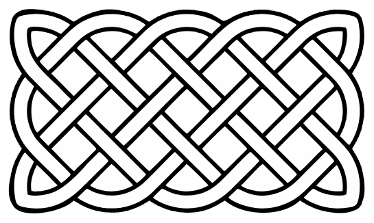
Figure 1: Sample of celtic knot projection to the plane (knot diagram).

Unknotting heavily tangled ropes, we are not even surprised that long threads, left to themselves, have the feature of entangled most unpleasant way of all. We are just a bitter sigh, when almost unravelled ball of wool accidentally falls into the clutches of a curious kitten, and our hard work goes to hell…

As a rule, we do not think about physical reasons for such ”injustice”, considering it as one of manifestations of the general law of life: unpleasant things happen more often than pleasant ones, and the sandwich usually falls butter side down. And we are quite aware that the spontaneous knotting of long strands, managed by the laws of probability theory, is a consequence of non-Euclidean geometry of the phase space of knots, i.e., such hypothetical space that contains all possible knots and in which there is a concept of the metric, or the distance between ”topologically similar” knots. The more different topological types of two knots, the greater the distance between them in this space. In general, the construction of this space, called the universal covering, and the description of its properties is extremely challenging. However, for some special cases, to which I address a little later, this space can be exhaustively described in geometric terms. So, it turns out that, in order to untie ropes in a purely scientific way, one has first to understand the Lobachevsky-Riemann geometry and its relation to the knot theory, and then to learn how the probability theory works in this non-Euclidean space. Before going further, let me briefly digress and discuss some of physical questions in which the topological interactions play a crucial role.

Mathematicians, primarily are interested in the question how to construct characteristics of entangled curves, that depend only on their topological state, but not on their shapes. Besides the traditional fundamental topological issues concerning the construction of new knot invariants, description of knot homologies, homotopic classes etc, there exists an important set of adjoint but much less studied problems related to probability theory and statistical physics. First of all, I mean the problem of so-called ”knot entropy” evaluation. Suppose we know everything about a set of entangled curves and know how to classify their topology. In order to understand which issue is interesting for physicists, imagine that one has a sample of rubber, i.e. the collection of polymer chains crosslinked at their extremities such that they form a connected network. When the network is deformed as shown in the Fig.2, the ensemble of available conformations of each individual subchain in the network changes, resulting in an essential decrease of the entropy, $S$. So, one says, that the elasticity of stretched rubber is of entropic nature.

Figure 2: Emotional view on elastic deformation. This sculpture, displayed at the Ujazdowski Castle s Center for Contemporary Art in Warsaw (Poland), was made by Agnieszka Kalinowska in 2002.

Once being prepared, the network sample cannot change its topology, i.e. is topologically frozen. If the applied deformations do not break the subchains, the topological constraints like entanglements between different subchains, at high extensions enter into the game as new effective quasi-links, providing additional restrictions on the ensemble of available subchain conformations. Therefore, the topological constraints contribute to the stress-strain dependence of polymeric networks, being the origin of so-called Mooney-Rivlin corrections to the classical Hook’s law grosberg-khokhlov .

In general, the non-phantomness of a polymer chain causes two types of interactions: i) volume interactions vanishing for infinitely thin chains, and ii) topological interactions, which survive even for chains of zero thickness. For sufficiently high temperatures, a polymer molecule strongly fluctuates without a reliable thermodynamic state called a coil state. However for temperatures below some critical value, $\theta$, the polymeric chain forms a weakly fluctuating dense globular (drop-like) structure grosberg-khokhlov , and one may expect that just in the globular state the topological interaction manifest themselves in all their glory. The crucial difficulty in description of topological interactions comes from their non-locality: the entropic part of a polymeric chain free energy, $F=-TS$, strongly depends on the global chain topology. Saying more formal, the topological interactions in dense polymer systems cannot be treated in a perturbative way and new ideas of nonperturbative description are demanded.

The general problem we are dealing with, can be formulated as follows. Consider a 3D cubic grid, and let $\Omega$ be the ensemble of all possible closed non-self-intersecting $N$-step paths on this grid with one point fixed. Denote by $\omega$ ($\omega\in\Omega$) some particular realization a path. We are aimed to calculate the partition function, $Z\{{\rm Inv}\}$, for a knot to be in a specific topological state characterized by the topological invariant ${\rm Inv}$ (yet non-specified). This can be written formally as

$$Z\{{\rm Inv}\}=\sum\limits_{\{\omega\in\Omega\}}\Delta\Big{\{}{\rm Inv}(\omega)-{\rm Inv}\Big{\}}$$ (1)

where ${\rm Inv}(\omega)$ is a functional representation of the invariant for the path $\omega$, $\rm Inv$ is a specific topological invariant of the knot which we would extract, and $\Delta$ is the Kronecker delta-function. The entropy, $S\{{\rm Inv}\}$, of a topological state, ${\rm Inv}$, is defined as

$$S\{{\rm Inv}\}=\ln Z\{{\rm Inv}\}$$ (2)

Based on the above definition, we can see that the statistical-topological problems are similar to those encountered in physics of disordered systems and in particular, of spin glasses. Indeed, the topological state of a path plays the role of a ”quenched disorder” and the entropy, $S\{{\rm Inv}\}$, is averaged over the ensemble of trajectories fluctuating at the ”quenched topological state” ne-gr1 . In the context of this analogy, it seems challenging to extend the concepts and methods developed over the years for disordered systems to the scopes of statistical topology. The main difference between the systems with topological disorder and the standard spin systems with disorder in the coupling constant, deals with the strongly nonlocal character of interactions in the first case: a topological state is determined for the entire closed path and is its ”global” property.

Below I review few conceptual steps in analytic description of topological interactions, which constitute the basis of a new interdisciplinary branch in mathematical physics, emerged at the edge of topology and statistical physics of fluctuating non-phantom rope-like objects. This new branch is called statistical (or probabilistic) topology. Yet its most fascinating manifestation is connected with the nonperturbative description of DNA packing in chromosomes in a form of a crumpled globule gns ; gr-rab . After experimental works of the MIT-Harvard team in 2009 mirny , the concept of crumpled globule became a kind of a new paradigm allowing to understand the mathematical origin of many puzzled features of DNA structuring and functioning in a human genome.

To intrigue the reader, I can say that the mathematical background of the crumpled globule deals with the statistics of Brownian bridges in the non-Euclidean space of constant negative curvature. Forthcoming sections are written to uncover this abracadabra.

II Milestones

II.1 Abelian epoch

In 1967 S.F. Edwards laid the foundation of the statistical theory of topological interactions in polymer physics. In edwards he proposed the way of exact computation of the partition function of a single self-intersecting random walk topologically interacting with the infinitely long uncrossible string (in 3D), or obstacle (in 2D). Sir Sam Edwards was the first to recognize the deep analogy between Abelian topological problems in statistical mechanics of Markov chains and quantum-mechanical problems (like Bohm-Aharonov ones) of the charged particles in the magnetic field. The review of classical results is given in physical context in wiegel , some rigorous results, including application in financial mathematics were discussed in yor , and modern advantages are summarized in grosberg-frisch . The works of S.F. Edwards opened the ”Abelian” epoch in the statistical theory of topological interactions.

In his work S.F. Edwards used the path integral formalism combined with the functional representation of the Gaussian linking number. All these steps have been many times reproduced in the literature, so we do not discuss the details, just remind that one finally arrives at the quantum problem of a free charged particle (with an imaginary magnetic charge) in a solenoidal magnetic field. If the magnetic flux (the obstacle) is located at the origin and is orthogonal to the plane, then for the probability $P(r_{1},r_{N},\theta,n,N)$ to find a $N$-step polymer chain, whose extremities are located at the distances $r_{1}$ and $r_{N}$ with $\widehat{{\bf r}_{1},{\bf r}_{N}}=\theta$ and which made $n$ full turns around the origin, we get:

$$P(r_{1},r_{N},\theta,n,N)=\frac{e^{-\frac{r_{1}^{2}+r_{N}^{2}}{2Na^{2}}}}{\pi Na^{2}}\int_{-\infty}^{\infty}d\nu I_{|\nu|}\left(\frac{r_{1}^{2}+r_{N}^{2}}{2Na^{2}}\right)e^{i\nu(2\pi n+\theta)}$$ (3)

where $I_{|\nu|}(...)$ is the modified Bessel function of order $|\nu|$, and $a$ is the size of the monomer (the typical step of the random walk). Obviously, the normalization condition is fulfilled,

$$\sum_{n=-\infty}^{\infty}P(r_{1},r_{N},\theta,n,N)=\frac{e^{-\frac{({\bf r}_{1}-{\bf r}_{N})^{2}}{Na^{2}}}}{\pi Na^{2}}$$ (4)

which means that the summation over all windings, $n$, $(-\infty<n<\infty)$ gives the Gaussian distribution. I will reproduce the result (9) in the next Section using the conformal approach. Though it is less popular in polymer physics than the path-integral formalism, it can be straightforwardly generalized to the non-Abelian multi-obstacle case.

It should be noted that the exact computation of the partition function of the self-intersecting random walk topologically entangled with two uncrossible obstacles in the plane, despite the huge number of works since 1967, still is an open problem. However, apparently this gap will be filled soon, because its quantum-mechanical counterpart, the Abelian problem of Bohm-Aharonov scattering in presence of two magnetic fluxes in the plane, has been solved in 2015 by E. Bogomolny bogom . To my point of view, his solution has opened the Pandora’s Box in the field, since he showed the deep mathematical connection of this particular problem to the theory of Painleve equations, integrable systems etc.

II.2 Non-Abelian epoch

Each time when we consider statistics of sufficiently dense polymer system, we encounter the extremely difficult problem of classification of topological states of polymer chains. Even the simplest physically relevant questions dealing with the knotting probability of a polymer chains, cannot be answered using the Gauss invariant due to its weakness. The Gauss linking number, becomes inapplicable since it does not reflect the sequence in which a given topological state was formed. For example, when some trial trajectory encloses two obstacles, the path is entangled with two obstacles simultaneously, while being not entangled with them separately, as shown in the Fig.3.

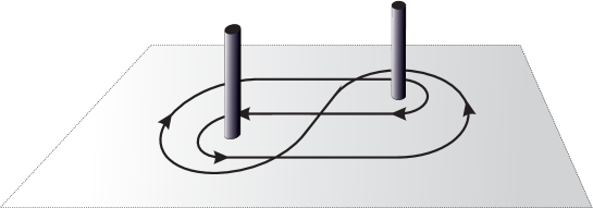
Figure 3: Topological configuration entangled with two obstacles simultaneously but not entangled with them separately (so-called Pochhammer contour).

Interestingly, I have not found in the literature any example of the path entangled with three obstacles simultaneously, while not entangled with any separate obstacle and any pairs of obstacles. Formally the question can be formulated as follows: find the element $X\in F_{3}$ of a free group of three generators, $F_{3}$, such that $X$ belongs both to the commutant of $F_{3}$ and to the commutant of commutant of $F_{3}$.

For dense polymer systems, one encounters many configurations as shown in the Fig.3, and they should be properly classified and treated using the invariants stronger than the Gauss linking number. So, to summarize, the Abelian (commutative) invariants become inapplicable for dense polymers and should be replaced by the non-Abelian (noncommutative) ones.

II.2.1 Methods of algebraic topology in polymer statistics. Topology as quenched disorder

A very useful and powerful method of knots classification has been offered by a polynomial invariant introduced by Alexander in 1928. The breakthrough in the field of polymer statistics was made in 1975-1976 when the algebraic polynomials were used for the topological state identification of closed random walks generated by the Monte-Carlo method volog . It has been recognized that the Alexander polynomials being much stronger invariants than the Gauss linking number, could serve as a convenient tool for the calculation of the thermodynamic properties of entangled random walks. To my point of view, 1975 is the year of the second birth of the probabilistic polymer topology, since the main part of our modern knowledge on knots and links statistics in dense polymer systems is obtained with the help of these works and their subsequent developments.

Other polynomial invariants for knots and links were suggested by V.F.R. Jones Jones (Jones polynomials) and by J. Hoste, A. Ocneanu, K. Millett, P.J. Freyd, W.B.R. Lickorish, and D.N. Yetter homfly (HOMFLY polynomials). The Jones invariant arise from the investigation of the topological properties of braids Birman . V.F.R. Jones succeeded in finding a profound connection between the braid group relations and the Yang-Baxter equations representing a necessary condition for commutativity of the transfer matrix offered the relation with integrable systems collect . It should be noted that neither the Alexander, Jones, and HOMFLY invariants, nor their various generalizations are complete, however these invariants are successfully used to solve many statistical problems in polymer physics. A clear geometric meaning of Jones invariant was provided by the works of Kauffman, who demonstrated that Jones invariant can be rewritten in terms of the partition function of the Potts spin model kauffman . Later Kauffman and Saleur showed that the Alexander invariants are related to a partition function of the free fermion model Kauf_Sal . The list of knot invariants used in polymer physics would be incomplete without mentioning Vassiliev invariants vassiliev and Khovanov homologies khovanov .

II.2.2 How to define the knot complexity?

There are many definitions of knot complexity. Some authors use the concept of minimal number of crossings tait ; bangert ; whit1 ; quake ; sheng . In other works (see, for example whit1 ; whit2 ) knot complexity is associated with a properly normalized logarithm of a kind of knot torsion, $\log|\Delta_{K}(-1)|$, where $\Delta_{K}(t)$ is the Alexander polynomial of the knot $K$. The estimate of knot complexity using the knot energy was discussed in the works freedman ; rolfsen ; sossinsky and to my point of view is yet underappreciated concept by polymer physicists.

Another approach deals with the fashionable concept of knot inflation id_kn . This topological invariant is defined as the quotient, $\mu$, of the contour length of the knot made of an elastic tube to its diameter in the maximal uniformly inflated configuration as shown in the Fig.4 for two different torus knots of same tube length. One sees that as more complex the knot, as thinner the limiting tube. Such approach was introduced and exploited in gr-rab ; id_kn .

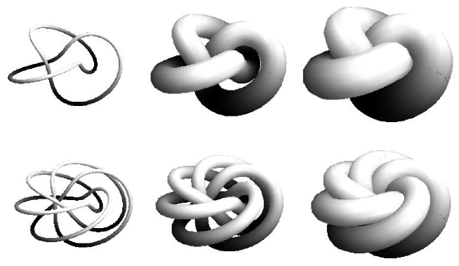
Figure 4: Affine inflation of a torus knot.

Knot invariants like the minimal number of crossings, as well as those built on the basis of the knot inflation concept, are similar to the invariants defined as the degree of algebraic polynomial used in the works grne_alg2 ; vasne . All of them have one common ancestor – the so-called primitive path, appeared in physical literature in 1970s in the works on entanglements in polymer melts. Introduced by P. de Gennes (see, for example gennes ), the primitive path was served to describe topological effects in the dynamics of individual chains in concentrated polymer solutions. Later on, the same concept has been used in the computation of equilibrium properties of polymer chains in lattices of topological obstacles ne_kh ; rub (I discuss this issue in details in the next Section).

The notion of a primitive path and its relation to the knot inflation concept can be elucidated as follows. Consider a closed path of fixed length entangled with the lattice of obstacles (see Fig.5a). Performing an affine extension (inflation) of the lattice of obstacles (preserving the length of the path), one arrives eventually at the unfolded fully stretched configuration , see the Figs.5b-c. Just the configuration in the Fig.5c is called the primitive path and it characterizes the topological state of a path with respect to the lattice of obstacles. Let us associate the properly normalized length of the chain and the spacing between obstacles, with the length of an elastic tube in the ”knot inflation concept” and its diameter. In that way, the relationship between the primitive path, the minimal number of crossings and the quotient $\mu$ in the maximal inflated tube configuration becomes intuitively clear by construction. In more details this relationship was discussed in gr-rab .

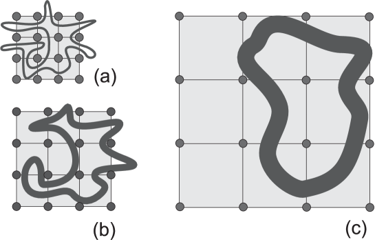
Figure 5: Affine inflation of a lattice of obstacles. The corresponding contour becomes ”less folded”.

In 1991 it was realized nesin2 that the concept of a primitive path has a straightforward interpretation in terms of a geodesics in a space of constant negative curvature. In the forthcoming section, we show how the geodesic length, in turn, may be related via its matrix representation to the degree of the polynomial invariant. Though our construction is restricted to the particular case of knots on narrow strips, the very idea can be used to attack more general models. The relationship between primitive paths and the maximal degree of the corresponding polynomial invariants has been discussed in jktr and will be overviewed in the next Section.

II.2.3 Conformal methods in statistics of entangled random walks

In 1985-1988 we have adopted the knowledge of stochastic processes in the Riemannian geometry to the statistical topology of polymers in multi-punctured spaces ne_kh ; nech-sem ; nechJPA . In particular, we have shown that the probability for a random walk (a polymer chain without volume interactions) to be unentangled with the regular lattice of topological obstacles in the plane is asymptotically described by the probability to form a Brownian bridge (BB) in the Lobachevsky plane (the non-Euclidean plane with a constant negative curvature). To have a transparent geometric image, though rather naive, the problem can be formulated as a ”snake in a night forest”. Suppose that very long snake, lost in a dense forest at night, would like to grasp randomly its own tale in such a way, that the formed ring is not entangled with any tree. What is the probability, $P(L,d)$, of such event, if $L$ is the length of the snake and $d$ is the average distance between the trees? What is the typical size, $R_{g}(N,d)$, of the snake (in polymer statistics, where a closed snake is replaced by a polymer ring, $R_{g}$ is called the ”gyration radius”)?

Conformal methods provide straightforward answer to these questions. The key idea is to find the conformal transformation $w(z)$ which maps the complex plane, $z=x+iy$, with obstacles (branching points), to the ”universal covering” space, $w=u+iv$, free of branchings in any finite domain. The main ingredient of this approach is the ”conformal invariance” of Laplace operator, $\Delta(z)$. Under the conformal mapping $w(z)$ the Laplacian $\Delta(z)=\partial^{2}_{xx}+\partial^{2}_{yy}$ is transformed to $\Delta(w)=\partial^{2}_{uu}+\partial^{2}_{vv}$ as follows

$$\Delta(w)=\partial^{2}_{uu}+\partial^{2}_{vv}=|w^{\prime}(z)|^{2}(\partial^{2}_{xx}+\partial^{2}_{yy})$$ (5)

where $w^{\prime}(z)=\frac{dw(z)}{dz}$. Define also $z(w)$, the inverse function of $w(z)$. If we are lucky enough and found the desired conformal mapping $w(z)$, then, in the universal covering space, our initial topological problem looks formally extremely simple: we have just to solve the diffusion-like equation in time $t$ with the diffusion coefficient $D$:

$$\partial_{t}P(w,t)-D|z^{\prime}(w)|^{-2}(\partial^{2}_{uu}+\partial^{2}_{vv})P(w,t)=\delta(w-w_{0})\delta(t)$$ (6)

without any topological constraints since all information about the topology is encoded now in the boundary conditions of the corresponding Cauchy problem in the covering space $w$. In the theory of stochastic processes the equation (6) describes the diffusion in the ”lifted” time, since it can be considered as a standard diffusion in the new metric-dependent time $T$, where $\partial_{T}=|z^{\prime}(w)|^{2}\partial_{t}$. However the simplicity of (6) in majority of cases is rather illusory: finding conformal mapping $z(w)$, and then solving (6) analytically, both these tasks are challenging problems. Despite, few nontrivial cases can be treated and solved at least asymptotically.

To demonstrate how the method of conformal mappings works, let us return to the Abelian problem and reconsider entanglement of the random walk with the single obstacle in the plane. Place the obstacle (the branching point) at the origin, make a cut along the positive part of the $x$-axis of the complex plane $z=x+iy$ as shown in the Fig. 6 and perform a conformal transform with the function $w(z)=\ln z$ to the universal covering space $w=u+iv$.

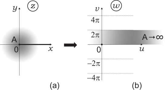
Figure 6: Conformal mapping of a plane with one branching point (obstacle) to the multi-sheet universal covering plane.

By elementary computations we get:

$$\begin{cases}u=\ln|z|\equiv\ln\rho,\quad v=\arg z;\vskip 6.0pt plus 2.0pt minus 2.0pt\\ |z^{\prime}(w)|^{-2}=e^{-2u}\end{cases}$$ (7)

If the path ${\cal C}$ makes $n$ full turns around the branching point in $z$, it means that in the $w$-plane the distance between extremities of the image of ${\cal C}$ along the $v$-axis is $2\pi n$. So, closed paths crossing the cut in $z$ are transformed into the open paths in $w$. The Cauchy problem in the lifted space is periodic in $v$ and in each Riemann sheet (the strip of width $2\pi$ in the plane $w$) can be written as follows

$$\begin{cases}\partial_{t}P(u,v,t)-D\,e^{-2u}(\partial^{2}_{uu}+\partial^{2}_{vv})P(u,v,t)\vskip 6.0pt plus 2.0pt minus 2.0pt\\ P(u_{0},v_{0},t)=\delta(u-u_{0})\delta(v-v_{0})\delta(t)\end{cases}$$ (8)

where $\delta(...)$ is the Dirac $\delta$-function. Making use of the substitution $\rho=e^{u}$ and taking into account the periodicity in $v$, we can rewrite (8) in the following form

$$\partial_{t}P(\rho,v,t)+D\left(\partial^{2}_{\rho\rho}+\frac{\partial_{\rho}}{\rho}+\frac{\partial^{2}_{vv}}{\rho^{2}}\right)P(\rho,v,t)=\frac{\delta(\rho-\rho_{0})}{(\rho\rho_{0})^{1/2}}\delta(v-v_{0})\delta(t)$$ (9)

Seeking the solution of (9) in the form

$$P(\rho,v,t)=\sum_{m=-\infty}^{\infty}P_{m}e^{im(v-v_{0})}$$ (10)

we get for $P_{m}$ the expression

$$P_{m}=\frac{1}{\pi ta^{2}}e^{-\frac{\rho_{0}^{2}-\rho^{2}}{ta^{2}}}I_{|\nu+m|}\left(\frac{2\rho\rho_{0}}{ta^{2}}\right)$$ (11)

were we have taken into account the expression for the diffusion coefficient in form $D=\frac{a^{2}}{4}$. Since

$$\sum_{m=-\infty}^{\infty}e^{im(v-v_{0})}=2\pi\sum_{n=-\infty}^{\infty}\delta(v+2\pi n-v_{0})$$ (12)

we arrive at (3), where we should made the replacements $\theta\leftrightarrow v$ and $N\leftrightarrow t$.

Now we are in position to attack our favorite problem – finding the probability that the random walk of length $t$ not entangled with respect to the triangular lattice of obstacles in the complex plane $z$, as shown in the Fig. 7a. To solve the problem, we should construct the conformal mapping of the multi-punctured plane $z$ to the universal covering space free of obstacles $w$ and take the corresponding Jacobian of transformation, $|z(w)|^{-2}$. In this particular case finding such a mapping is more elaborated task than for one-punctured plane, though still doable. The conformal mapping $z(w)$ of the flat equilateral triangle $ABC$ located in $z$ onto the zero-angled triangle $ABC$ in $w$, is constructed in three sequential steps, shown in the Fig. 7a-d.

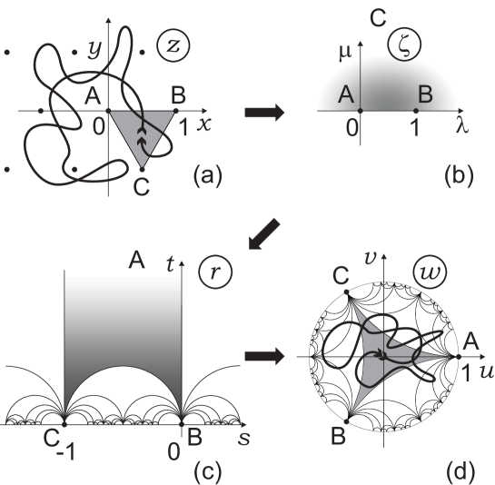
Figure 7: Conformal mapping $z(w)$ is realized as a composition of three mappings: $z(\zeta)$ [(a)–(b)], $\zeta(r)$ [(b)–(c)], and $r(w)$ [(c)–(d)]. Finally we have $z(\zeta(r(w)))$.

First, we map the triangle $ABC$ in $z$ onto the upper half-plane $\zeta$ of auxiliary complex plane $\zeta$ with three branching points at 0, 1 and $\infty$ – see the Fig. 7a-b. This mapping is realized by the function $z(\zeta)$:

$$z(\zeta)=\frac{\Gamma(\frac{2}{3})}{\Gamma^{2}(\frac{1}{3})}\int_{0}^{\zeta}\frac{d\xi}{\xi^{2/3}(1-\xi)^{2/3}}$$ (13)

with the following coincidence of branching points:

$$\left\{\begin{array}[]{lcl}A(z=0)&\leftrightarrow&A(\zeta=0)\vskip 6.0pt plus 2.0pt minus 2.0pt\\ B(z=1)&\leftrightarrow&B(\zeta=1)\vskip 6.0pt plus 2.0pt minus 2.0pt\\ C(z=e^{-i\frac{\pi}{3}})&\leftrightarrow&C(\zeta=\infty)\end{array}\right.$$ (14)

Second step consists in mapping the auxiliary upper half-plane $\textrm{Im}\,\zeta>0$ onto the circular triangle $ABC$ with angles $\{\alpha,\alpha,0\}$ – the fundamental domain of the Hecke group hecke in $r$, where we are intersted in the specific case $\{\alpha,\alpha,0\}=\{0,0,0\}$ – see Fig. 7b-c. This mapping is realized by the function $\zeta(r)$, constructed as follows koppenfels . Let $\zeta(r)$ be the inverse function of $r(\zeta)$ written as a quotient

$$r(\zeta)=\frac{\phi_{1}(\zeta)}{\phi_{2}(\zeta)}$$ (15)

where $\phi_{1,2}(\zeta)$ are the fundamental solutions of the 2nd order differential equation of Picard-Fuchs type:

$$\zeta(\zeta-1)\phi^{\prime\prime}(\zeta)+\big{(}(a+b+1)\zeta-c\big{)}\phi^{\prime}(\zeta)+ab\phi(\zeta)=0$$ (16)

Following caratheodory ; koppenfels , the function $r(\zeta)$ conformally maps the generic circular triangle with angles $\{\alpha_{0}=\pi|c-1|,\alpha_{1}=\pi|a+b-c|,\alpha_{\infty}=\pi|a-b|\}$ in the upper halfplane of $w$ onto the upper halfplane of $\zeta$. Choosing $\alpha_{\infty}=0$ and $\alpha_{0}=\alpha_{1}=\alpha$, we can express the parameters $(a,b,c)$ of the equation (16) in terms of $\alpha$, taking into account that the triangle $ABC$ in the Fig. 7c is parameterized as follows $\{\alpha_{0},\alpha_{1},\alpha_{\infty}\}=\{\alpha,\alpha,0\}$ with $a=b=\frac{\alpha}{\pi}+\frac{1}{2},c=\frac{\alpha}{\pi}+1$. This leads us to the following particular form of equation (16)

$$\zeta(\zeta-1)\phi^{\prime\prime}(\zeta)+\Big{(}\frac{\alpha}{\pi}+1\Big{)}\big{(}2\zeta-1\big{)}\phi^{\prime}(\zeta)+\Big{(}\frac{\alpha}{\pi}+\frac{1}{2}\Big{)}^{2}\phi(\zeta)=0$$ (17)

where $\alpha=\frac{\pi}{m}$ and $m=3,4,...\infty$. For $\alpha=0$ Eq.(17) takes an especially simple form, known as Legendre hypergeometric equation golubev ; hille . The pair of possible fundamental solutions of Legendre equation are

$$\begin{array}[]{l}\phi_{1}(\zeta)=F\big{(}\frac{1}{2},\frac{1}{2},1,\zeta\big{)}\vskip 6.0pt plus 2.0pt minus 2.0pt\\ \phi_{2}(\zeta)=iF\big{(}\frac{1}{2},\frac{1}{2},1,1-\zeta\big{)}\end{array}$$ (18)

where $F(...)$ is the hypergeometric function. From (15) and (18) we get $r(\zeta)=\frac{\phi_{1}(\zeta)}{\phi_{2}(\zeta)}$. The inverse function $\zeta(r)$ is the so-called modular function, $k^{2}(r)$ (see golubev ; hille ; jacobi2 for details). Thus,

$$\zeta(r)\equiv k^{2}(r)=\frac{\theta_{2}^{4}(0,e^{i\pi r})}{\theta_{3}^{4}(0,e^{i\pi r})}$$ (19)

where $\theta_{2}$ and $\theta_{3}$ are the elliptic Jacobi $\theta$-functions jacobi2 ; mum ,

$$\begin{array}[]{l}\displaystyle\theta_{2}\left(\chi,e^{i\pi w}\right)=2e^{i{\pi\over 4}r}\sum_{n=0}^{\infty}e^{i\pi rn(n+1)}\cos(2n+1)\chi\vskip 6.0pt plus 2.0pt minus 2.0pt\\ \displaystyle\theta_{3}\left(\chi,e^{i\pi r}\right)=1+2\sum_{n=0}^{\infty}e^{i\pi rn^{2}}\cos 2n\chi\end{array}$$ (20)

and the correspondence of branching points in the mapping $\zeta(r)$ is as follows

$$\left\{\begin{array}[]{lcl}A(\zeta=0)&\leftrightarrow&A(r=\infty)\vskip 6.0pt plus 2.0pt minus 2.0pt\\ B(\zeta=1)&\leftrightarrow&B(r=0)\vskip 6.0pt plus 2.0pt minus 2.0pt\\ C(\zeta=\infty)&\leftrightarrow&C(r=-1)\end{array}\right.$$ (21)

Third step, realized via the function $r(w)$, consists in mapping the zero-angled triangle $ABC$ in $r$ into the symmetric triangle $ABC$ located in the unit disc $w$ – see Fig. 7c-d. The explicit form of the function $r(w)$ is

$$r(w)=e^{-i\pi/3}\frac{e^{2i\pi/3}-w}{1-w}-1$$ (22)

with the following correspondence between branching points:

$$\left\{\begin{array}[]{lcl}A(r=\infty)&\leftrightarrow&A(w=1)\vskip 6.0pt plus 2.0pt minus 2.0pt\\ B(r=0)&\leftrightarrow&B(w=e^{-2\pi i/3})\vskip 6.0pt plus 2.0pt minus 2.0pt\\ C(r=-1)&\leftrightarrow&C(w=e^{2\pi i/3})\end{array}\right.$$ (23)

Collecting (13), (19), and (22) we arrive at the following expression for the derivative of composite function,

$$z^{\prime}(\zeta(r(w)))=z^{\prime}(\zeta)\,\zeta^{\prime}(r)\,r^{\prime}(w)$$ (24)

where ^′ stands for the derivative. We have explicitly:

$$z^{\prime}(\zeta)=\frac{\Gamma(\frac{2}{3})}{\Gamma^{2}(\frac{1}{3})}\,\frac{\theta_{3}^{16/3}(0,\zeta)}{\theta_{2}^{8/3}(0,\zeta)\;\theta_{0}^{8/3}(0,\zeta)}$$

and

$$\zeta^{\prime}(r)|=i\pi\frac{\theta_{2}^{4}\;\theta_{0}^{4}}{\theta_{3}^{4}};\qquad i\frac{\pi}{4}\theta_{0}^{4}=\frac{d}{d\zeta}\ln\left(\frac{\theta_{2}}{\theta_{3}}\right)$$

The identity

$$\theta^{\prime}_{1}(0,e^{i\pi\zeta})\equiv\left.\frac{d\theta_{1}(\chi,e^{i\pi\zeta})}{d\chi}\right|_{\chi=0}\\ =\pi\theta_{0}(\chi,e^{i\pi\zeta})\,\theta_{2}(\chi,e^{i\pi\zeta})\,\theta_{3}(\chi,e^{i\pi\zeta})$$ (25)

enables us to write

$$\left|z^{\prime}(r)\right|^{2}=h^{2}\left|\theta^{\prime}_{1}\left(0,e^{i\pi r}\right)\right|^{8/3}$$ (26)

where $h=\left(\frac{16}{\pi}\right)^{1/3}\frac{\Gamma(\frac{2}{3})}{\Gamma^{2}(\frac{1}{3})}\approx 0.325$, and

$$\theta_{1}(\chi,e^{i\pi r})=2e^{i\frac{\pi}{4}r}\sum_{n=0}^{\infty}(-1)^{n}e^{i\pi n(n+1)r}\sin(2n+1)\chi$$ (27)

Differentiating (22), we get

$$r^{\prime}(w)=\frac{i\sqrt{3}}{(1-w)^{2}}$$

and using this expression, we obtain the final form of the Jacobian of the composite conformal transformation $J(z(\zeta(r(w))))$:

$$J(z(w))=|z^{\prime}(w)|^{2}=3h^{2}\frac{|\eta(r(w))|^{8}}{|1-w|^{4}}$$ (28)

where

$$\eta(r)=\big{(}\theta_{1}^{\prime}(0,e^{i\pi r})\big{)}^{1/3}$$

is the Dedekind $\eta$-function

$$\eta(w)=e^{\pi iw/12}\prod_{n=0}^{\infty}(1-e^{2\pi inw})\quad(w=u+iv)$$ (29)

and the function $r(w)$ is defined in (22).

Thus, we arrive at the diffusion equation in the unit disc $|w|<1$:

$$\partial_{t}P(w,t)-\frac{a^{2}}{4}J(z(w))\big{(}\partial^{2}_{uu}+\partial^{2}_{vv}\big{)}P(w,t)=\delta(w-w_{0})\delta(t)$$ (30)

with the function $J(z(w))$ given by (28). The probability to find the two-dimensional random walk unentangled with the lattice of obstacles after time $t$, is given by the solution of Eq.(30), where we should plug at the very end $w=w_{0}=0$. The probability of returning to the same point $w_{0}=0$ in the initial Riemann sheet (the gray triangle in the Fig. 7d) ensures that the trajectory is: i) closed, and ii) ”contractible” (i.e. topologically trivial with respect to the lattice of obstacles).

Exact solution of (30) is unknown, however its asymptotic behavior we can extract relying on modular properties of Dedekind $\eta$-function (29). Consider the normalized Jacobian, defined as follows:

$$f(w)=J(z(w))\big{(}1-(u^{2}+v^{2})\big{)}^{2}$$ (31)

where $|z|=\sqrt{u^{2}+v^{2}}$ and $\psi={\rm arg}\,z$ are radial and angular coordinates in the Poincare unit disc disc $|w|<1$. In the Fig. 8 we have shown the density plot of the function $f(w)$ within the unit disc $|w|<1$ for $f(w)>f_{0}=0.15$. As one can see from the Fig. 8, the function $f(w)$ has identical local maxima in all the centers of circular triangles shown in the Fig. 7d. Thus, we conclude that the Jacobian $J(z(w))$ in the centers of circular cells (domains) coincides with the metric of the Lobachevsky plane in the Poincaré disc,

$$ds^{2}=\frac{du^{2}+dv^{2}}{\big{(}1-(u^{2}+v^{2})\big{)}^{2}}$$ (32)

Note that the profile shown in the Fig. 8 has striking similarities with the 3-branching Cayley tree and can be interpreted as a ”continuous Cayley tree”.

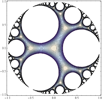
Figure 8: Density plot of the function $f(w)$ (see (31)) above the level $f_{0}=0.15$.

If we slightly modify our random walk model, we can exploit the connection with the Lobachevsky geometry. Namely, consider the random walk which stays in the vicinity of the center of a circular cell and then rapidly jumps to the center of the neighboring cell, stays there, then jumps again, and so forth… Such a random jumping process we can approximately describe by the diffusion in the Poincare disc with the Lobachevsky plane metric (32) and the diffusion coefficient ${\cal D}$:

$$\partial_{t}P(w,t)-{\cal D}\big{(}(1-(u^{2}+v^{2})\big{)}^{2}\big{(}\partial^{2}_{uu}+\partial^{2}_{vv}\big{)}P(w,t)=\delta(u)\delta(v)\delta(t)$$ (33)

Making use of the change of variables $(r,\psi)\to(\rho,\psi)$, where $\rho=\ln\frac{1+r}{1-r}$, we get the unrestricted random walk on the surface of the one-sheeted hyperboloid, ${\cal H}$ obtained by the stereographic projection from the Poincaré unit disc. Correspondingly the probability $P(\rho,t)$ reads

$$P(\rho,t)=\frac{e^{-\frac{t{\cal D}}{4}}}{4\pi\sqrt{2\pi(t{\cal D})^{3}}}\int_{\rho}^{\infty}\frac{\xi\exp\left(-\frac{\xi^{2}}{4t{\cal D}}\right)}{\sqrt{\cosh\xi-\cosh\rho}}d\xi$$ (34)

The physical meaning of the geodesic length, $\rho$, on ${\cal H}$ is straightforward: $\rho$ is the length of the primitive path in the lattice of obstacles, i.e. the length of the shortest trajectory remaining after all topologically allowed contractions of the random path in the lattice of obstacles. Hence, $\rho$ can be considered a non-Abelian topological invariant, more powerful than the Gauss linking number. This invariant is not complete except one point, $\rho=0$, where it precisely classifies the paths belonging to the trivial homotopic class in the lattice of obstacles.

II.2.4 Group-theoretic methods in statistics of entangled random walks

Non-Abelian entanglement of the path with two obstacles on the plane can be treated in the group-theoretic setting. Let us associate the generators $g_{1}$ and $g_{2}$ with the clockwise full turns around obstacles 1 and 2 respectively, and the inverse generators $g_{1}^{-1}$ and $g_{2}^{-2}$ – around the counterclockwise turns around 1 and 2, as shown in the Fig. 9. Suppose that $g_{1},g_{2},g_{1}^{-1},g_{2}^{-1}$ are the generators of the free group $\Gamma_{2}$ which by definition has no commutation relations. Thus, the possible contractions in the group $\Gamma_{2}$ are $g_{1}g_{1}^{-1}=g_{1}^{-1}g_{1}=g_{2}g_{2}^{-1}=g_{2}^{-1}g_{2}=I$, where $I$ is the identity element.

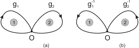
Figure 9: Generators of free group $\Gamma_{2}$.

Any closed path entangled with the obstacles 1 and 2 can be topologically presented by a word written in terms of generators $g_{1},g_{2},g_{1}^{-1},g_{2}^{-1}$. For example, the Pochhammer contour shown in the Fig. 3 reads: $g_{1}g_{2}g_{1}^{-1}g_{2}^{-1}$. Since the group $\Gamma_{2}$ is noncommutative (non-Abelian), we have $g_{1}g_{2}\neq g_{2}g_{1}$, thus we cannot exchange the sequence of letters and replace $g_{1}g_{2}$ by $g_{2}g_{1}$. However, in the commutative (Abelian) group generated by the set $\{f_{1},f_{2},f_{1}^{-1},f_{2}^{-1}\}$, we can do so, since $f_{1}f_{2}=f_{2}f_{1}$, and the Pochhammer contour in the Abelian representation becomes contractible: $f_{1}f_{2}f_{1}^{-1}f_{2}^{-1}=f_{2}\underbracket{f_{1}f_{1}^{-1}}_{I}f_{2}^{-1}=\underbracket{f_{2}f_{2}^{-1}}_{I}=I$.

Suppose now that we have a set ${\cal S}=\{g_{1},g_{2},g_{1}^{-1},g_{2}^{-1}\}$ and rise random words of $N$ letters by sequential adding of generators from the set ${\cal S}$. Each generator in ${\cal S}$ we take with the probability $p=\frac{1}{4}$. We are interested in computing the partition function $Z_{N}(x)$ for all $N$-letter random words to have the irreducible (”primitive”) word of $x$ letters. The partition function $Z_{N}(0)$ gives the number of $N$-letter words that are completely reducible (i.e. unentangled) with the obstacles 1 and 2. The word counting problem in the free group $\Gamma_{2}$ can be visualized as the trajectories (built by sequential adding of letters) on the 4-branching Cayley tree shown in the Fig. 10a. The irreducible (primitive) word is the shortest ”bare” path along the tree connecting the extremities of the trajectory.

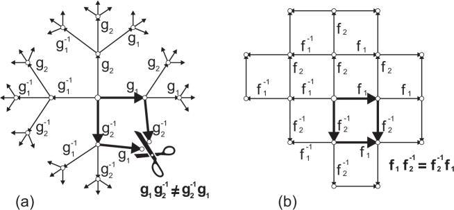
Figure 10: Visualization of commutation relations in commutative (a) and in free (b) groups.

The partition function, $Z_{N}(x)$, of all $N$-step paths on the 4-branching Cayley tree, starting at the origin and ending at some distance $x$ from it, satisfies the following recursion relation

$$\left\{\begin{array}[]{rcll}\displaystyle Z_{N+1}(x)&=&3Z_{N}(x-1)+Z_{N}(x+1),&\quad x\geq 2\vskip 6.0pt plus 2.0pt minus 2.0pt\\ \displaystyle Z_{N+1}(x)&=&4Z_{N}(x-1)+Z_{N}(x+1),&\quad x=1\vskip 6.0pt plus 2.0pt minus 2.0pt\\ Z_{N+1}(x)&=&Z_{N}(x+1),&\quad x=0\vskip 6.0pt plus 2.0pt minus 2.0pt\\ Z_{N}(x)&=&0,&\quad x\leq-1\vskip 6.0pt plus 2.0pt minus 2.0pt\\ Z_{N=0}(x)&=&\delta_{x,0},\end{array}\right.$$ (35)

where $x$ is the distance (the bare path) from the root of the Cayley graph, measured in number of generations of the tree. By making a shift $x\to x+1$, one can rewrite (35) as

$$\left\{\begin{array}[]{rcll}Z_{N+1}(x)&=&3Z_{N}(x-1)+Z_{N}(x+1)+\delta_{x,2}\,Z_{N}(x-1),&\qquad x\geq 1\vskip 6.0pt plus 2.0pt minus 2.0pt\\ Z_{N}(x)&=&0,&\qquad x=0\vskip 6.0pt plus 2.0pt minus 2.0pt\\ Z_{N=0}(x)&=&\delta_{x,1},\end{array}\right.$$ (36)

where $\delta_{x,y}$ is the Kronecker $\delta$–function: $\delta_{x,y}=1$ for $x=y$ and $\delta_{x,y}=0$ for $x\neq y$.

Equation (36) can be symmetrized by the substitution

$$Z_{N}(x)=A^{N}B^{x}W_{N}(x).$$ (37)

Selecting $A=B=\sqrt{3}$, we arrive at the equation

$$\left\{\begin{array}[]{rcll}W_{N+1}(x)&=&\displaystyle W_{N}(x-1)+W_{N}(x+1)+\frac{1}{3}\,\delta_{x,2}\,W_{N}(x-1),&\qquad x\geq 1\vskip 6.0pt plus 2.0pt minus 2.0pt\\ W_{n}(x)&=&0,&\qquad x=0\vskip 6.0pt plus 2.0pt minus 2.0pt\\ W_{N=0}(x)&=&\displaystyle\frac{\delta_{x,1}}{\sqrt{3}}\end{array}\right.$$ (38)

Introducing the generating function

$${\cal W}(s,x)=\sum_{N=0}^{\infty}W_{N}(x)s^{n}\qquad\left(W_{N}(x)=\frac{1}{2\pi i}\oint{\cal W}(s,x)s^{-N-1}\,ds\right)$$ (39)

and its $\sin$–Fourier transform

$$\tilde{{\cal W}}(s,q)=\sum_{x=0}^{\infty}{\cal W}(s,x)\sin qx\qquad\left({\cal W}(s,x)=\frac{2}{\pi}\int_{0}^{\pi}\tilde{{\cal W}}(s,q)\sin qx\,dq\right),$$ (40)

one obtains from (38)

$$\frac{\tilde{{\cal W}}(s,q)}{s}-\frac{\sin q}{s\sqrt{p-1}}=2\cos q\,\tilde{{\cal W}}(s,q)+\frac{2}{\pi}\frac{1}{3}\sin 2q\int_{0}^{\pi}\tilde{{\cal W}}(s,q)\sin q\,dq.$$ (41)

Solving (41) and performing the inverse Fourier transform, we arrive at the following explicit expression for the generating function ${\cal W}(s,x)$:

$${\cal W}(s,x)=\frac{2}{\pi}\int_{0}^{\infty}\tilde{{\cal W}}(s,q)\sin qx\,dq\\ =\frac{1}{s\sqrt{3}}\left(\frac{1-\sqrt{1-4s^{2}}}{2s}\right)^{x}\left(1+\frac{2\left(1-\sqrt{1-4s^{2}}\right)}{12s^{2}-1\left(1-\sqrt{1-4s^{2}}\right)^{2}}\right).$$ (42)

Since, by definition, $Z_{N}(x)=A^{N}B^{x}W_{N}(x)$ (see (37)), we can write down the relation between the generating functions of $Z_{N}(x)$ and of $W_{N}(x)$:

$${\cal Z}(\lambda,x)=\sum_{N=0}^{\infty}Z_{N}(x)\lambda^{N}=\sum_{N=0}^{\infty}A^{N}B^{x}W_{N}(x)\lambda^{N}=B^{x}{\cal W}(\lambda A,x).$$ (43)

Thus,

$${\cal Z}(\lambda,x)=3^{x/2}{\cal W}(\lambda\sqrt{3},x),$$ (44)

where ${\cal W}(\lambda\sqrt{3},x)$ is given by (42) and we should substitute $\lambda\sqrt{3}$ for $s$. The partition function, ${\cal Z}(\lambda,x)$, of the random walk ensemble reads

$${\cal Z}(\lambda,x)=\frac{6\lambda\left(\frac{\displaystyle 1-\sqrt{1-4\lambda^{2}(p-1)}}{\displaystyle 2\lambda}\right)^{x}}{18\lambda^{2}-\left(1-\sqrt{1-12\lambda^{2}}\right)}.$$ (45)

For the grand partition function of all trajectories returning to the origin, ${\cal Z}(\lambda)\equiv{\cal Z}(\lambda,x=0)$, we get the following expression

$${\cal Z}(\lambda)=\frac{6\lambda}{18\lambda^{2}-\left(1-\sqrt{1-12\lambda^{2}}\right)}.$$ (46)

To extract the asymptotic behavior of the partition function $Z_{N}$ (the number of trajectories returning to the origin after $N$ steps, one should perform the inverse transform similar to (39)

$$Z_{N}=\frac{1}{2\pi i}\oint{\cal Z}(\lambda)\lambda^{-N-1}d\lambda\sim\frac{\left(2\sqrt{3}\right)^{N}}{N^{3/2}}$$ (47)

As it should be, the probability to return to the origin on a 4-branching Cayley tree, $Z_{N}/(4^{N})$ is exponentially small.

Let us note some striking topological similarity between the Cayley tree structure of the noncommutative group $\Gamma_{2}$ shown in the Fig. 9 and the metric structure of the modular group, visualized in the Fig. 7. This similarity is not occasional. Having the graph of the group $\Gamma_{2}$, we can ask the question in which Riemann surface the graph of the group $\Gamma_{2}$ can be isometrically embedded. The answer is that the Cayley tree is the graph of isometries (one of many) of the Lobachevsky plane (the Riemann surface of constant negative curvature). This is schematically depicted in the Fig. 11 where the chips (the saddle) is the example of the surface with constant negative Gaussian curvature. Contrary to that, the commutative group $\{f_{1},f_{2},f_{1}^{-1},f_{2}^{-1}\}/[f_{1}f_{2}=f_{2}f_{1}]$ isometrically covers the planar square lattice – see the Fig. 10b.

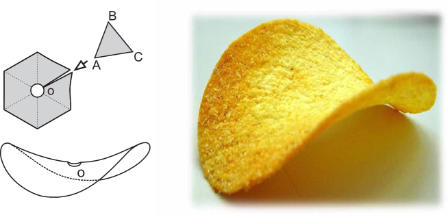
Figure 11: Isometric embedding of the free group into the Lobachevsky plane (Riemann surface of constant negative curvature).

II.2.5 Conditional Brownian bridges in Hyperbolic spaces

The result formulated in this Section is the central point, connecting statistics of random walks in Hyperbolic spaces and the topology of knotted random walks. There are few different incarnations of one and the same question concerning the conditional return probability of the symmetric random walk in the Hyperbolic geometry:

(i) For the problem of the conditional paths counting on the Cayley tree, we are interested in the following question. Let $Z_{N}(x)$ be the number of $N$-step path on the Cayley tree starting from the origin and ending at some distance $x$ measured in number of the tree generations (”coordinational spheres”) from the root point. Let the paths starting from the tree root, reach the distance $x$ after $M$ steps, and then return to the origin at the very last step, $N$. The corresponding conditional distribution, $P(x,M,N)$ we can compute as follows

$$P(x,M,N)=\frac{Z_{M}(x)Z_{N-M}(x)}{Z_{M}(0)V(x)}$$ (48)

The expression (48) means that the entire $N$-step Brownian bridge (the path returning to the origin) consists of two independent parts: the $M$-step part of the path form the root point to some point located at the distance $x$, and $N-M$-step part of the path from the root point again to some point located at the distance $x$. Now we have to ensure that the ends of these two $M$– and $N-M$–parts coincide at the point ${\bf x}$. The factor $V(x)$ in the denominator of (48) is the number of different points located at the distance $x$ from the root of the tree, $V(x)=4\times 3^{x-1}$ for the 4-branching Cayley tree. Thus, $Z_{M}(x)V^{-1}(x)$ is the probability that the $M$-step part ends in some specific point ${\bf x}$. Substituting expressions for $Z_{M}(x)$, $Z_{N-M}(x)$, $Z_{N}(0)$ in (48), we arrive at the following asymptotic form of $P(x,M,N)$ at $x\gg 1$:

$$P(x,M,N)\sim\sqrt{\frac{N}{2\pi M(N-M)}}e^{x^{2}\left(\frac{1}{2M}+\frac{1}{2(N-M)}\right)}$$ (49)

Computing $\left<x^{2}\right>$ with the function $P(x,M,N)$, we get

$$\bar{x}=\sqrt{\left<x^{2}\right>}=\frac{\sum_{x=0}^{\infty}x^{2}P(x,M,N)}{\sum_{x=0}^{\infty}}=\sqrt{\frac{M(N-M)}{N}}$$ (50)

As one sees, for any $M=cN$ ($c={\rm const}$, $0<c<1$), the average distance $\bar{x}$ has the behavior typical for an ordinary random walk,

$$\bar{x}=\sqrt{a(1-a)}\sqrt{N}$$ (51)

Thus, the typical behavior of intermediate points of the Brownian bridge on the Cayley tree is statistically the same as on the one-dimensional lattice, i.e. the drift on the tree which occurs due to asymmetry of the random walk (the probability to go from the root is larger than the probability to come back to the root) is completely compensated. This is the key point for existence of topologically nontrivial crumpled globule structure, which will be discussed in the following Section.

(ii) Consider now the asymptotics of the conditional Brownian bridge in the Lobachevsky plane. Construct the desired conditional probability, $W(x,M,N)$ as follows

$$W(\rho,\tau,t)=\frac{P(\rho,\tau)P(\rho,t-\tau)}{P(0,t)}v(\rho)$$ (52)

where $P(\rho,t)$ defines the probability that the random path after time $t$ ends in the specific point located at the distance $\rho$ of the Labachevsky plane, and $v(\rho)=\sinh\rho$ is the circumference of circle of radius $\rho$ in the Lobachevsky plane.

The diffusion equation for the density $P({\bf q},t)$ of the free random walk on a Riemann manifold is governed by the Beltrami-Laplace operator:

$$\partial_{t}P({\bf q},t)={\cal D}\frac{1}{\sqrt{g}}\frac{\partial}{\partial q_{i}}\left(\sqrt{g}\left(g^{-1}\right)_{ik}\frac{\partial}{\partial q_{k}}\right)P({\bf q},t)$$ (53)

where

$$\begin{array}[]{c}\displaystyle P({\bf q},t=0)=\delta({\bf q})\vskip 6.0pt plus 2.0pt minus 2.0pt\\ \displaystyle\int\sqrt{g}P({\bf q},t)d{\bf q}=1\end{array}$$ (54)

and $g_{ik}$ is the metric tensor of the manifold; $g=\det g_{ik}$. For the Lobachevsky plane one has

$$||g_{ik}||=\left|\left|\begin{array}[]{cc}1&0\vskip 6.0pt plus 2.0pt minus 2.0pt\\ 0&\sinh^{2}\rho\end{array}\right|\right|$$ (55)

where $\rho$ stands for the geodesics length in the Lobachevsky plane. The corresponding diffusion equation now reads

$$\partial_{t}P(\rho,\varphi,t)={\cal D}\left(\partial^{2}_{\rho\rho}+\coth\rho\partial_{\rho}+\frac{1}{\sinh^{2}\rho}\partial^{2}{\varphi\varphi}\right)P_{p}(\rho,\varphi,t)$$ (56)

The radially symmetric solution of Eq.(56) is

$$\begin{array}[]{lll}P(\rho,t)&=&\displaystyle\frac{e^{-\frac{t{\cal D}}{4}}}{4\pi\sqrt{2\pi(t{\cal D})^{3}}}\int_{\rho}^{\infty}\frac{\xi\exp\left(-\frac{\xi^{2}}{4t{\cal D}}\right)}{\sqrt{\cosh\xi-\cosh\rho}}d\xi\vskip 6.0pt plus 2.0pt minus 2.0pt\\ &\simeq&\displaystyle\frac{e^{-\frac{t{\cal D}}{4}}}{4\pi t{\cal D}}\left(\frac{\rho}{\sinh\rho}\right)^{1/2}\exp\left(-\frac{\rho^{2}}{4t{\cal D}}\right)\end{array}$$ (57)

(compare to (42)). Substituting (57) into (52), we get for the conditional probability $W(\rho,\tau,t)$ the following asymptotic expression

$$W(\rho,\tau,t)=\frac{N}{4\pi{\cal D}\tau(t-\tau)}\rho\exp\left\{-\frac{\rho^{2}}{4{\cal D}}\left(\frac{1}{\tau}+\frac{1}{t-\tau}\right)\right\}$$ (58)

Hence we again reproduce the Gaussian distribution function with zero mean.

(iii) Equations (49) and (58) describing the conditional distributions Brownian bridges on the Cayley tree and on the Riemann surface of constant negative curvature, have direct application to the conditional distributions of Lyapunov exponents for products of non-commutative matrices. Consider for specificity the random walk on the group $SL(2,R)$. Namely, we multiply sequentially $N$ random matrices $M_{j}=\left(\begin{array}[]{cc}a_{j}&b_{j}\\ c_{j}&d_{j}\end{array}\right)\in SL(2,R)$, whose entries $\{a_{i},b_{j},c_{j},d_{j}\}$ are randomly distributed for any $j=1,...,N$ in some finite support subject to the relation $a_{j}d_{j}-b_{j}c_{j}=1$. Thus we have a product of random matrices

$$Q(N)=\left(\begin{array}[]{cc}a_{1}&b_{1}\\ c_{1}&d_{1}\end{array}\right)\left(\begin{array}[]{cc}a_{2}&b_{2}\\ c_{2}&d_{2}\end{array}\right)...\left(\begin{array}[]{cc}a_{M}&b_{M}\\ c_{M}&d_{M}\end{array}\right)...\left(\begin{array}[]{cc}a_{N}&b_{N}\\ c_{N}&d_{N}\end{array}\right)$$ (59)

The asymptotic $N\to\infty$ behavior of the largest eigenvalue, $\Lambda_{N}$ of the typical (i.e. averaged over different samples) value of $Q(N)$ is ensured by the Fürstenberg theorem furstenberg1963noncommuting , which states that

$$\Lambda_{N}\sim e^{\delta_{1}N}$$ (60)

where $\delta_{1}$ is the group– and measure–specific, though $N$-independent ”Lyapunov exponent”.

Motivated by examples (i) and (ii), consider the conditional Brownian bridge in the space of matrices, i.e. consider such products $Q(N)$ that are equal to the unit matrix and ask about the typical behavior of the largest eigenvalue of first $M$ as shown below:

$$\overbracket{\left(\begin{array}[]{cc}a_{1}&b_{1}\\ c_{1}&d_{1}\end{array}\right)\left(\begin{array}[]{cc}a_{2}&b_{2}\\ c_{2}&d_{2}\end{array}\right)...\left(\begin{array}[]{cc}a_{M}&b_{M}\\ c_{M}&d_{M}\end{array}\right)}^{\Lambda_{M}=?}...\left(\begin{array}[]{cc}a_{N}&b_{N}\\ c_{N}&d_{N}\end{array}\right)=\left(\begin{array}[]{cc}1&0\\ 0&1\end{array}\right)$$ (61)

The answer to this question is as follows: $\Lambda_{M}=e^{\delta_{2}\sqrt{\frac{M(N-M)}{N}}}$ i.e. for $M=cN$ ($0<c<1$), one has

$$\Lambda_{M}=e^{\delta_{3}\sqrt{N}}$$ (62)

where we have absorbed the constants in $\delta_{3}=\delta_{2}\sqrt{a(1-a)}$. The proof of the corresponding theorem using the method of large deviations, can be found in nesin2 , however the result (62), which holds for random walks on any noncommutative group, is easy to understand qualitatively. It is sufficient to recall that the Lobachevsky plane $H$ can be identified with the group $SL(2,R)/SO(2)$. Thus, the Brownian bridge on the group $SL(2,R)/SO(2)$, can be viewed either as the conditional random walk governed by the Beltrami-Laplace operator, or as the product of random matrices.

We arrive at the following conclusion. The Brownian bridge condition for random walks in the space of constant negative curvature makes the curved space effectively flat and turns the corresponding conditional distribution for the intermediate time moment of random walks to the Gaussian distribution with zero mean. This result is very general and can be applied to random walks on various noncommutative groups, such as modular group, $SL(n,R)$, braid groups $B_{n}$, etc. This result is crucial in our further discussions of the crumpled state of collapsed unknotted polymer chain.

II.3 Crumpled globule: Topological correlations in collapsed unknotted rings

In 1988 we have theoretically predicted the new condensed state of a ring unentangled and unknotted macromolecule in a poor solvent. We named this state ”the crumpled globule” and studied its unusual fractal properties gns . That time our arguments were rather hand-waving and more solid understanding came essentially later, around 2005 vasne ; jktr . As we shall show, the most striking physical arguments of the estimation of the degree of entanglement of a part of a long unknotted random trajectory confined in a small box are provided by the statistics of conditional Brownian bridges in the space of constant negative curvature.

First of all one has to define the topological state of a part of a ring polymer chain. As we discussed in the Introduction, mathematically rigorous definition of the topological state exists for closed or infinite paths only. However, the everyday’s experience tells us that open but sufficiently long rope can be knotted. Hence, it is desirable to introduce a concept of a quasiknot available for topological description of open paths. For the first time the idea of quasiknots in a polymer context had been formulated by I.M. Lifshits and A.Yu. Grosberg ligr . They argued that the topological state of a linear polymer chain in a collapsed (globular) state is defined much better than topological state of a random coil. Actually, the distance between the ends of the chain in a globule is of order $R\sim aN^{1/3}$, where $a$ is a size of a monomer and $N$ is a number of monomers in a chain. Taking into account that $R$ is sufficiently smaller than the contour length $N$ and that the density fluctuations in the globular state are negligible, we may define the topological state of a path in a globule as a topological state of composite trajectory consisting of a chain itself and a segment connecting its ends. This composite structure can be regarded as a quasiknot for an open chain in a collapsed state. Later we shall repeatedly use this definition.

The influence of topological constraints on statistical properties of polymers, namely, the random knotting probability, in confined geometries has been numerically considered in tesi , while the paper orlan has been devoted to the determination of the equilibrium entanglement complexity of polymer chains in melts. In the works jktr we made further step, considering the topological state of a part of ring unknotted polymer chain in a confined geometry, where the compact configuration of the polymer is modelled by dense lattice knots. The knot is called ”dense” if its projection onto the plane completely fills the rectangle lattice $M$ of size $L_{v}\times L_{h}$ as it is shown in the Fig. 12a, resembling the celtic knot in the Fig. 1. The lattice $M$ is filled densely by a single thread, which crosses itself in each vertex of the lattice in two different ways: ”up” or ”down”. The topology of a lattice diagram is defined by the up-down passages, and by the prescribed boundary conditions. The ”woven carpet” shown in Fig. 12a corresponds to a trivial knot. To avoid any possible confusions, we apply our model to the polymer ring located in a thin slit between two horizontal plates as it is shown in Fig. 12b. It is evident that the ring chain in a thin thin slit becomes a quasi two-dimensional system. Our lattice model is oversimplified (even for the polymer chain in a thin slit) because it does not take into account the spatial fluctuations of a knotted polymer chain. However, we expect that our model properly describes the condensed (globular) structure of a polymer ring because the chain fluctuations in the globule are essentially suppressed and the chain has reliable thermodynamic structure with a constant density ligr .

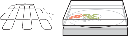
Figure 12: (a) Random woven carpet corresponding to the trivial knot; (b) Dense knot confined in a thin slit.

We are interested in the following statistical-topological question inspired by the conditional Brownian bridge ideology. Define at each intersection of vertical and horizontal threads (i.e. in each ”lattice vertex”) $k$ the random variable $\varepsilon_{k}$, taking values

$$\varepsilon_{k}=\begin{cases}+1&\mbox{for "up" crossing}\\ -1&\mbox{for"down" crossing}\end{cases}$$ (63)

The set of independently generated quenched random variables $\{\varepsilon_{1},...,\varepsilon_{N}\}$ in all vertices of the lattice diagram, together with the boundary conditions, define the knot topology.

Suppose that we consider such sub-ensemble of crossings $\{\varepsilon_{1},...,\varepsilon_{N}\}$ that corresponds to the trivial entire (”parent”) knot. Let us cut a part of a parent trivial knot and close open ends of the threads as it is shown in Fig. 13. This way we get the well defined ”daughter” quasiknot. We are interested in the typical topological state of daughter quasiknots under the condition that the parent knot is trivial. I think, the reader can feel in this formulation the flavor of conditional Brownian bridges…

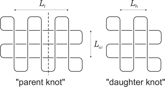
Figure 13: (a) Trivial ”parent” knot; (b) ”Daughter” knot obtained by cutting a part of the parent knot.

The averaged knot complexity, $n$, understood as the minimal number of crossings on the knot diagram, for the unconditional random knotting of knot diagram behaves as $n\sim N$ where $N$ is the initial size of the lattice knot. By the semi-analytic and semi-numeric arguments we have shown in jktr that the typical conditional complexity, $n^{*}$, of the daughter knot of size $M$ behaves as $n^{*}\sim\sqrt{\frac{M(N-M)}{N}}$ and for $M=cN$ $(0<c<1)$, $N\gg 1$, has the asymptotic behavior

$$n^{*}\sim\sqrt{a(1-a)}\sqrt{N}$$ (64)

Thus, each macroscopic part of a dense lattice trivial knot is weakly knotted (compared to the unconditional random knotting).

In 2015 we have performed in nech-mirny extensive Monte-Carlo simulations for self-avoiding polymer chains in confined geometry in 3D space. The role of topological constraints in the equilibrium state of a single compact and unknotted polymer remains unknown. Previous studies gns ; gr-rab have put forward a concept of the crumpled globule as the equilibrium state of a compact and unknotted polymer. In the crumpled globule, the subchains were suggested to be space-filling and unknotted. Recent computational studies examined the role of topological constraints in the non-equilibrium (or quasi-equilibrium) polymer states that emerge upon polymer collapse mirny ; rost ; obukhov2 ; chu ; chertovich2014crumpled . This non-equilibrium state, often referred to as the fractal globule mirny ; leonid_review , can indeed possess some properties of the conjectured equilibrium crumpled globule. The properties of the fractal globule, its stability schiessel , and its connection to the equilibrium state are yet to be understood.

Elucidating the role of topological constraints in equilibrium and non-equilibrium polymer systems is important for understanding the organization of chromosomes. Long before experimential data on chromosome organization became available mirny , the crumpled globule was suggested as a state of long DNA molecules inside a cell gr-rab . Recent progress in microscopy cremer2011review and genomics dekker_NRG provided new data on chromosome organization that appear to share several features with topologically constrained polymer systems rosa_everaers ; mirny ; grosberg2012review . For example, segregation of chromosomes into territories resembles segregation of space-filling rings gr-krem2 ; smrek ; stasiak , while features of intra-chromosomal organization revealed by Hi-C technique are consistent with a non-equilibrium fractal globule emerging upon polymer collapse mirny ; leonid_review ; machine or upon polymer decondensation rosa_everaers . These findings suggest that topological constraints can play important roles in the formation of chromosomal architecture halverson2014melt .

In nech-mirny we have examined the role of topological constraints in the equilibrium state of a compact polymer. We performed the equilibrium Monte Carlo simulations of a confined unentangled polymer ring with and without topological constraints. Without topological constraints, a polymer forms a classical equilibrium globule with a high degree of knotting grosberg-khokhlov ; knots-kardar ; knots-kardar2 . A polymer is kept in the globular state by impenetrable boundaries, rather than pairwise energy interactions, allowing fast equilibration at a high volume density.

In the work nech-mirny we found that topological states of closed subchains (loops) are drastically different in the two types of globules and reflect the topological state of the whole polymer. Namely, loops of the unknotted globule are only weakly knotted and mostly unconcatenated. We also found that spatial characteristics of small knotted and unknotted globules are very similar, with differences starting to appear only for sufficiently large globules. Subchains of these large unknotted globules become asymptotically compact ($R_{G}(s)\sim s^{1/3}$), forming crumples. Analysis of the fractal dimension of surfaces of loops suggests that crumples form excessive contacts and slightly interpenetrate each other. Overall, in the the asymptotic limit (for very long chains) we have supported the conjectured crumpled globule concept gns . However, the results of nech-mirny also demonstrate that the internal organization of the unknotted globule at equilibrium differs from an idealized hierarchy of self-similar isolated compact crumples.

In the simulations a single homopolymer ring with excluded volume interactions was modelled on a cubic lattice and confined into a cubic container at a volume density $0.5$. The Monte Carlo method with non-local moves (see nech-mirny and references therein) allowed us to study chains up to $N=256\,000$. If monomers were prohibited to occupy the same site, this Monte Carlo move set naturally constrains topology, and the polymer remains unknotted. The topological state of a loop was characterized by $\varkappa$, the logarithm of the Alexander polynomial evaluated at $-1.1$ gr-krem2 ; knots-kardar ; knots-kardar2 . To ensure equilibration, we estimated the scaling of the equilibration time with $N$ for $N\leq 32\,000$, extrapolated it to large $N$, and ran simulations of longer chains, $N=108\,000$ and $256\,000$, to exceed the estimated equilibration time. We also made sure that chains with topological constraints remain completely unknotted through the simulations, while polymers with relaxed topological constraints become highly entangled.

To understand the role of topological correlations, we asked how the topological state of the whole polymer influences the topological properties of its subchains. Because a topological state can be rigorously defined only for a closed contour, we focused our analysis on loops, i.e. subchains with two ends occupying neighboring lattice sites. The Fig. 14a presents the average knot complexity $\langle\varkappa(s)\rangle$ for loops of length $s$ for both types of globules. We found that loops of the knotted globule were highly knotted, with the knot complexity rising sharply with $s$. Loops of the unknotted globule, on the contrary, were weakly knotted, and their complexity increased slowly with $s$.

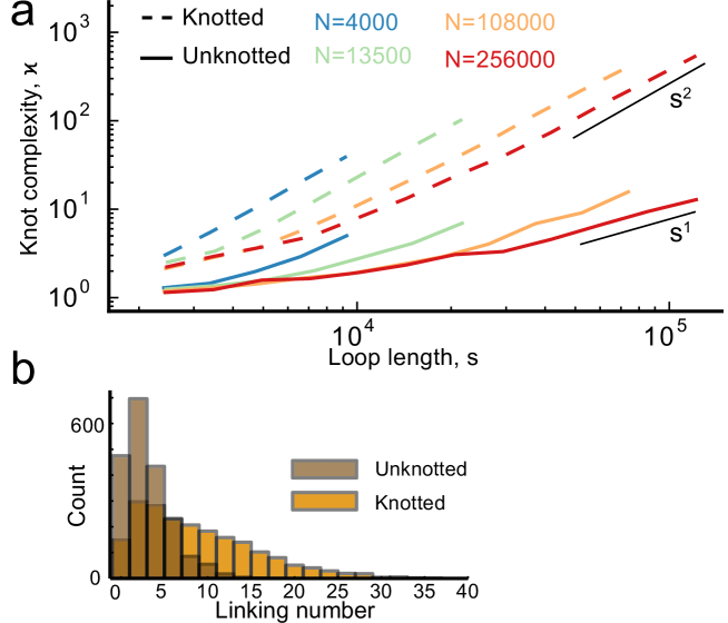
Figure 14: Topological properties of polymer loops in the knotted and unknotted globules. (a) Knot complexity of polymer loops as a function of their length, $s$, for chains of different length $N$ (shown by colors) in knotted (dashed) and unknotted (solid) globules. (b) Distribution of the linking numbers for non-overlapping loops of length $s=9000$ to $11\,000$ in $32\,000$-long globules.

This striking difference in the topological states of loops for globally knotted and unknotted chains is a manifestation of the general statistical behavior of so-called matrix–valued Brownian Bridges (BB) jktr . The knot complexity $\varkappa$ of loops in the topologically unconstrained globule is expected to grow as $\varkappa(s)\sim s^{2}$. In contrast, due to the global topological constraint imposed on the unknotted globule, the knot complexity of its loops grows slower, $\varkappa(s)\sim s$, which follows from the statistical behavior of BB in spaces of constant negative curvature (see the Fig. Fig. 15a, and vasne ; jktr for details).

Another topological property of loops of a globule is the degree of concatenation between the loops. We computed the linking number for pairs of non-overlapping loops in the knotted and crumpled (unknotted) globules, and found that loops in the unknotted globule are much less concatenated than loops in the knotted globule. Taken together, these results show that the topological state of the whole (parent) chain propagates to the daughter loops. While loops of the unknotted globule are still slightly linked and knotted, their degree of entanglement is much lower than for the loops in the topologically relaxed knotted globule.

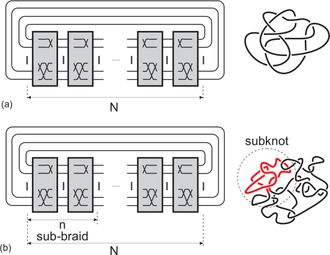
Figure 15: Schematic representation of knots by braids: a) unconditional random distribution of black boxes produces a very complex knot; b) conditional distribution implies the whole knot to be trivial, which imposed strong constraints on complexity of any subpart of the braid.

Our topological problem to determine the complexity of a subloop in a globally trivial collapsed polymer chain allows natural interpretation in terms of Brownian bridges. Suppose the following imaginative experiment. Consider the phase space $\Omega$ of all topological states of densely packed knots on the lattice. Select from $\Omega$ the subset $\omega$ of trivial knots. To simplify the setting, consider a knot represented by a braid, as shown in the Fig. 15, where the braid is depicted by a sequence of uncorrelated ”black boxes” (each black box contains some number of up- and down-crossings. If crossings in all black boxes are identically and uniformly distributed, then the boxes are statistically similar. Cut a part of each braid in the subset $\omega$, close open tails and investigate the topological properties of resulting knots. Just such situation has been qualitatively studied in vasne ; jktr . The crumpled globule hypothesis states the following: if the whole densely packed lattice knot is trivial, then the topological state of each of its ”daughter” knot is almost trivial. We have shown that the computation of the knot complexity in the braid representation depicted in the Fig. 15 can be interpreted as the computation of the highest eigenvalue of the product of noncommutative matrices designated by black boxes.

To proceed, consider first the typical (unconditional) complexity of a knot represented by a sequence of $N$ independent black boxes. This question is similar to the growth of the logarithm of the largest eigenvalue, $\Lambda$, of the product of $N$ independent identically distributed noncommutative random matrices. According to the Fürstenberg theorem furstenberg1963noncommuting , in the limit $N\gg 1$ one has

$$\ln\Lambda(N)\sim\gamma_{1}N,$$ (65)

where $\gamma_{1}={\rm const}$ is the so-called Lyapunov exponent (compare to (60)). Being rephrased for knots, this result means that the average knot complexity, $\varkappa$, understood as a minimal number of crossings, $M$, necessary to represent a given knot by the compact knot diagram, extensively grows with $M$, i.e. $\varkappa\sim M$. In the ordinary globule, for subchains of length $N^{2/3}<s<N$, the typical number of crossing, $M$, on the knot diagram grows as $M\sim s^{2}$, leading to the scaling behavior for the knot complexity $\varkappa$:

$$\varkappa\sim s^{2}$$ (66)

This is perfectly consistent with the well known fact: the probability of spontaneous unknotting of a polymer with open ends in a globular phase is exponentially small. Following the standard scheme volog ; knots-kardar ; knots-kardar2 , we characterize the knot complexity, $\varkappa$, by the logarithm of the Alexander polynomial, $\ln[{\rm Al}(t=-1.1){\rm Al}(t=-1/1.1)]$, i.e. we set $\varkappa=\ln[{\rm Al}(t=-1.1){\rm Al}(t=-1/1.1)]$. As it seen from Fig. 14, the conjectured dependence $\ln{\rm Al}(t=-1.1)\sim s^{2}$ is perfectly satisfied for ordinary (knotted) globule.

Consider now the conditional distribution on the products of identically distributed black boxes. We demand the product of matrices represented by black boxes to be a unit matrix (topologically trivial). The question of interest concerns the typical behavior of $\ln\Lambda^{*}(M,N)$, where $\Lambda^{*}(M,N)$ is the largest eigenvalue of the sub-chain of first $M$ matrices in the chain of $N$ ones. The answer to this question is known nesin2 : if $n=cN$ ($0<c<1$ and $N\gg 1$), then

$$\ln\lambda^{*}(n=cN,N)\sim\sqrt{c(1-c)}\sqrt{N}=\gamma_{2}(c)\sqrt{N}$$ (67)

where $\gamma_{2}(c)$ absorbs all constants independent on $N$. Translated to the knot language, the condition for a product of $N$ matrices to be completely reducible, means that the ”parent” knot is trivial. Under this condition we are interested in the typical complexity $\varkappa^{*}$ of any ”daughter” sub-knot represented by first $n=cN$ black boxes.

Applying the (67) to the knot diagram of the unknotted globule, we conclude that the typical conditional complexity, $\varkappa^{*}$ expressed in the minimal number of crossings of any finite sub-chain of a trivial parent knot, grows as

$$\varkappa^{*}\sim\sqrt{s^{2}}\sim s$$ (68)

with the subchain size, $s$. Comparing (68) and (66), we conclude that subchains of length $s$ in the trivial knot are much less entangled/knotted than subchains of same lengths in the unconditional structure, i.e. when the constraint for a parent knot to be trivial is relaxed. Indeed, this result is perfectly supported by Fig. 14 which show linear grows of $\tilde{\varkappa}=\ln[{\rm Al}(t=-1.1)\,{\rm Al}(t=-1/1.1)]$ with $s$ for the unknotted globule, while quadratic grows for the knotted globule.

III Conclusion

III.1 The King is dead, long live The King!

The very concept of the crumpled (fractal) globule as of possible thermodynamic equilibrium state of an unknotted ring polymer confined in a small volume, appeared in 1988 in a joint work by A. Grosberg, S. Nechaev and E. Shakhnovich gns . Soon after, in 1993, A. Grosberg, Y. Rabin, S. Havlin, and A. Neer published a paper where they proposed the crumpled globule model to be a possible condensed state of DNA packing in a chromosome gr-rab . Then, over decades, the interest to the crumpled globule was moderate: it was considered as an interesting, though sophisticated artificial exercise. The attempts to find the crumpled structure in direct numeric simulations, or in real experiments on proteins or DNAs were not too convincing.

Still, few interesting exceptions, which fuelled some discussions around the crumpled globule, should be mentioned:

• the observation of the two-stage dynamics of collapse of the macromolecule after abrupt changing of the solvent quality, found in light scattering experiments by B. Chu and Q. Ying chu ;

• the experiments on compatibility enhancement in mixtures of ring and linear chains mck , the construction of the quantitative theory of a collapse of $N$–isopropilacrylamide gel in a poor water frac ;

• the experiments on superelasticity of polymer gels prepared in diluted solutions urayama ;

• the indications of observation of the crumpled globule in numerical simulations shakh ; borovin .

The breakthrough in the interest to the crumpled globule happen after the brilliant experimental work of the MIT-Harvard team in 2009 mirny . Immediately after, the concept of crumpled (fractal) globule became the candidate for the new paradigm explaining many realistic features the DNA packing and functioning in a human genome.

Analysis of chromatin folding in human genome based on a genome-wide chromosome conformation capture method (Hi-C) 3c ; mirny provides a comprehensive information on spatial contacts between genomic parts and imposes essential restrictions on available 3D genome structures. The experimental Hi-C maps obtained for various organisms and tissues mirny ; dixon ; drosoph ; mouse ; sofueva ; dekker_NRG ; bacteria display very rich structure in a broad interval of scales. The researchers pay attention to the average contact probability, ${\cal P}(s)$, between two units of genome separated by a genomic distance, $s$, which decays in typical Hi-C maps approximately as ${\cal P}(s)\sim 1/s$ (see mirny ).

The crumpled globule is a state of a polymer chain which in a wide range of scales is self-similar and almost unknotted, forming a fractal space-filling-like structure. Both these properties, self-similarity and absence of knots, are essential for genome folding: fractal organization makes genome tightly packed in a broad range of scales, while the lack of knots ensures easy and independent opening and closing of genomic domains, necessary for transcription gr-rab ; leonid_review . In a three-dimensional space such a tight packing results in a space-filling with the fractal dimension $D_{f}=D=3$. The Hi-C contact probability, $P_{i,j}$, between two genomic units, $i$ and $j$ in a $N$-unit chain, depends on a combination of structural and energetic factors. Simple mean-field arguments (see, for example, mirny ) demonstrate that in a fractal globule with $D_{f}=3$ the average contact probability, ${\cal P}(s)=(N-s)^{-1}\sum_{i=0}^{N-s}P_{i,i+s}$, between two units separated by the genomic distance $s=|i-j|$, decays as ${\cal P}(s)\sim s^{-1}$. It should be noted that recent numeric simulations gr-krem2 ; nech-mirny , and more sophisticated arguments beyond the mean-field approximation grosberg2012review ; grosb_softmatter , point out that the contact probability decays as ${\cal P}(s)\sim s^{-\gamma}$ with $\gamma\simeq 1.05-1.09$.

Despite the crumpled globule is our ”favorite child”, I should clearly state that it does not explain exhaustively all details of the chromatin folding and definitely should be combined with more refined models and concepts. Theoretical models of chromatin packing in the nucleus, which can possibly explain the observed behavior of intra-chromosome Hi-C contact maps, split roughly into two groups. The first group of works relies on specific interactions within the chromatin, like loop or bridge formation, loops1 ; loops2 ; loops3 ; loops4 ; loops5 ; pnas ; longowskiDif and these authors do not believe in crumpled globule, while the second group aims to explain the chromatin structure in terms of large-scale topological interactions gr-rab ; rosa_everaers ; mirny ; leonid_review ; grosberg2012review ; rosa_everaers2 ; grosb_softmatter ; nech-mirny ; onefifth based on the crumpled model of the polymer globule gns . For example, in nazarov we combined the assumption that chromatin can be considered as a heteropolymer chain with a quenched primary sequence filion , with the general hierarchical fractal globule folding mechanism. With this conjecture we were able to reproduce the large-scale chromosome compartmentalization, not assumed explicitly from the very beginning. To show the compatibility of the hierarchical folding of a crumpled globule with the fine structure of experimentally observed Hi-C maps, we suggested in nazarov a simple toy model based on the crumpled globule folding principles together with account of quenched disorder in primary sequence.

To summarize, my feeling of the current state of the art called ”the crumpled globule” is formulated in the title of this Section. All together we have come a long way from the nonperturbative description of topological constraints in collapsed polymer phase to real biophysical applications, we have understood on this way constructive connection of statistics of polymer entanglements with Brownian bridges in the non-Euclidean geometry, we have got new results for statistics of random braids, and finally we have explained some features of DNA packing in chromosomes. Keeping our eyes open, we clearly see that the appearance of new experimental results demonstrates that our initial topological arguments were too crude and too naive. However they gave birth of new understanding of the role of topology in genomics and have led to new ideas and methods which constitute the modern STATISTICAL TOPOLOGY OF POLYMERS.

III.2 Where to go?

I think we are only at the beginning of a highway, where the statistics of random walks is interwined with the geometric group theory, algebraic topology and integrable systems in mathematical physics, as well as has various incarnations in physics dealing with the crumpled globule concept. Let me name some but a few such directions.

I would like to mention random walks on braid groups, grows of random heaps, viewed as random sequential ballistic deposition (random ”Tetris game”). Introducing the concept of the ”locally free group” as an approximant of the braid group, one can solve exactly the word problem in the locally free group and obtain analytically the bilateral estimates (from above and from below) for the growth of the volume of the braid group $B_{n}$ for arbitrary $n$ 36 ; 45 ; 93 . Interesting new results beyond the mean-field approximation for entanglement of threads in random braids have been obtained recently in bunin .

Sequential ballistic deposition (BD) with the next-nearest-neighbor interactions in a $N$-column box can viewed as a time-ordered product of $N\times N$-matrices consisting of a single $sl_{2}$-block which has a random position along the diagonal. One can interpret the uniform BD growth as the diffusion in the symmetric space $H_{N}$. In particular, the distribution of the maximal height of a growing heap can be connected to the distribution of the maximal distance for the diffusion process in $H_{N}$, where the coordinates of $H_{N}$ can be interpreted as the coordinates of particles of the one-dimensional Toda chain. The group-theoretic structure of the system and links to some random matrix models was discussed in 82 .

As concerns the impact of crumpled globule concept in physics, we have demonstrated that folding and unfolding of a crumpled polymer globule can be viewed as a cascade of equilibrium phase transitions in a hierarchical system, similar to the Dyson hierarchical spin model. Studying the relaxation properties of the elastic network of contacts in a crumpled globule, we showed that the dynamic properties of hierarchically folded polymer chains in globular phase are similar to those of natural molecular machines (like myosin, for example). We discuss the potential ways of implementations of such artificial molecular machine in computer and real experiments, paying attention to the conditions necessary for stabilization of crumples under the fractal globule formation in the polymer chain collapse machine (see also the work on coalescence of crumples in polymer collapse kardar-bunin ).

The ability of crumpled globule to act as molecular machine definitely provokes a new angle on an eternal problem of the origin of life, related to overcoming the ”error threshold” in producing and selecting complex molecular structures during the prebiotic evolution avet1 . This permits us to put forward a conjecture about a possibility for the crumpled globule to be a sort of the ”primary molecular machine” naturally formed under the prebiotic conditions. The primary crumpled globule molecular machine (CGMM) made by polymers (not necessarily of biological nature), could perform some specific functions typical for true biological molecular machines. The diversity of CGMM may be concerned mainly with the attracting manifold, in which the CGMM action is performed. This allows for functional variability without altering the structural archetype. Certainly, the idea that crumpled globule could be the prebiotic molecular machine needs experimental verification. However, the results machine ; avet2 provide a rather optimistic view on the evolutionary scenarios in which the primary molecular machines, themselves, are taken out of the bio-molecular context. In this paradigm, the beginning of biological evolution is associated with the spontaneous appearance of complex functional systems of primary ”artificial” CGMM capable of performing collective reproduction and autonomous behavior, which then are replaced in evolution by more effective biomolecular systems. On this optimistic note I would like to end the story.

These notes are based on several lectures at the SERC School on Topology and Condensed Matter Physics (organized in 2015 by RKM Vivekananda University at S.N Bose National Center for Basic Sciences, Calcutta, India). I would thank Somen Bhattacharjee for kind invitation, opportunity to explore some wonderful places in India and strong push to arrange lectures as a written text. The topics discussed above summarize the subjects of millions conversations over many years with my friends and colleagues, Alexander Grosberg, Anatoly Vershik, Vladik Avetisov, Leonid Mirny, Michael Tamm. Particularly I would like to thank Maxim Frank-Kamenetskii and Alexander Vologodsky, whose nice review in 1981 fuelled my interest to polymer topology, and to Alexey Khokhlov with whom we got first results beyond the Abelian theory of polymer entanglements in 1985. The importance of conditional Brownian bridge concept in statistics of non-commutative random walks was recognized in joint work with Yakov Sinai in 1991. Especially I would like to highlight the role of Alexander Grosberg whose ironic and deep comments and ideas tease and support me for more than a quarter of century.

References

- (1) L.H. Kauffman, Topology, 26 395 (1987); L.H. Kauffman, AMS Contemp. Math. Series, 78 263 (1989); L.H. Kauffman, Knots and Physics (Singapore: WSPC, 1991)
- (2) A.Yu. Grosberg, A.R. Khokhlov, Statistical physics of macromolecules (New York: AIP Press, 1994)
- (3) A.Yu. Grosberg, S. Nechaev, J. Phys. A: Math. Gen., 25 4659 (1992)
- (4) A.Yu. Grosberg, S.K. Nechaev, E.I. Shakhnovich, J.Phys. (Paris), 49 2095 (1988)
- (5) A. Grosberg, Y. Rabin, S. Havlin and A. Neer, Europhys. Lett., 23, 373 (1993)
- (6) E. Lieberman-Aiden, N.L. van Berkum, L. Williams, M. Imakaev, T. Ragoczy, A. Telling, I. Amit, B.R. Lajoie, P.J. Sabo, M.O. Dorschner, et al, Science 326 289 (2009)
- (7) S.F. Edwards, Proc. Roy. Soc., 91 513 (1967)
- (8) F. Wiegel, Introduction to Path-Integrals Methods in Physics and Polymer Science (Singapore: WSPC, 1986)
- (9) M. Yor, J. Appl. Prob., 29 202 (1992); Math. Finance, 3 231 (1993)
- (10) A. Grosberg, H. Frisch, J. Phys. A: Math. Gen., 37 3071 (2004)
- (11) E. Bogomolny Scattering on two Aharonov-Bohm vortices, arXiv:1508.04616
- (12) A.V. Vologodskii, M.D. Frank-Kamenetskii, Usp. Fiz. Nauk, 134 641 (1981) (in Russian); A.V. Vologodskii, A.V. Lukashin, M.D. Frank-Kamenetskii, V.V. Anshelevich, Zh. Exp. Teor. Fiz., 66 2153 (1974); A.V. Vologodskii, A.V. Lukashin, M.D. Frank-Kamenetskii, Zh. Exp. Teor. Fiz., 67 1875 (1974); M.D. Frank-Kamenetskii, A.V. Lukashin, A.V. Vologodskii, Nature, 258 398 (1975)
- (13) V.F.R. Jones, Ann. Math., 126, 335 (1987); Bull. Am. Math. Soc., 12 103 (1985)
- (14) W.B.R. Likorish, Bull. London Math. Soc., 20 558 (1988); W.B.R. Lickorish, An Introduction to Knot Theory, Springer Serirs: Graduate texts in Mathematics (Springer: 1997)
- (15) J. Birman, Knots, Links and Mapping Class Groups, Ann. Math. Studies, 82 (Princeton Univ. Press, 1976)
- (16) Integrable Models and Strings, Lect. Not. Phys., 436 (Springer: Heidelberg, 1994); M. Wadati, T.K. Deguchi, Y. Akutsu, Phys. Rep., 180 247 (1989)
- (17) L.H. Kauffman, H. Saleur, Comm. Math. Phys., 141 293 (1991)
- (18) V.A. Vassiliev, Complements of Discriminants of Smooth Maps: Topology and Applications in Math. Monographs, 98 (Trans. AMS, 1992); D. Bar-Natan, Topology, 34 423 (1995)
- (19) M. Khovanov, A categorification of of the Jones Polynomial, arXiv:math.QA/9908171; D. Bar-Natan, J. Knot Theory Ramifications, 16 243 (2007)
- (20) P. Tait, Trans. Royal Soc. Edinburgh 28 145 (1877)
- (21) P.Bangert, M.Berger, R. Prandi, J. Phys. (A): Math. Gen., 35 43 (2002)
- (22) S.R. Quake, Phys. Rev. Lett., 73 3317 (1994)
- (23) Y. Sheng, P. Lai, Phys. Rev. E, 63 021506 (2001)
- (24) E. Janse van Rensburg, D. Sumners, E. Wasserman, S. Whittington, J. Phys. A: Math. Gen, 25 6557 (1992)
- (25) C. Soteros, D. Sumners, S. Whittington, Math. Proc. Camb. Phil. Soc., 111, 75 (1992)
- (26) M. Freedman, Z. He, Z. Wang, Ann. Math. 139 1 (1994)
- (27) A. Kholodenko, D. Rolfsen, J. Phys. (A): 29 5677 (1996)
- (28) O. Karpenkov, A.B. Sossinsky, Russ. J. Math. Phys., 18 306 (2011), arXiv:1106.3414
- (29) Ideal Knots, eds. A. Stasiak, V. Katrich, L.H. Kauffman, Series of Knots and Everything, 19 (WSPC: Singapore, 1998)
- (30) A.Yu. Grosberg, S. Nechaev, Europhys. Lett., 20 603 (1992)
- (31) O.A. Vasilyev, S.K. Nechaev, JETP, 93 1119 (2001); O.A. Vasilyev, S.K. Nechaev, Theor. Math. Phys., 134 142 (2003)
- (32) P.G. de Gennes, Scaling Concepts in Polymer Physics (Cornell Univ. Press: Ithaca, 1979)
- (33) E. Helfand, D. Pearson, J. Chem. Phys., 79 2054 (1983); M. Rubinstein, E. Helfand, J. Chem. Phys., 82 2477 (1985)
- (34) A. Khokhlov, S. Nechaev, Phys. Lett. (A) 112 156 (1985)
- (35) S. Nechaev, Ya.G. Sinai, Bol. Soc. Bras. Mat., 21 121 (1991)
- (36) S. Nechaev, O. Vasilyev, J. Knot Theory Ramifications, 14 243 (2005); S. Nechaev, O. Vasilyev, Thermodynamics and topology of disordered knots: Correlations in trivial lattice knot diagrams, in Physical and Numerical Models in Knot Theory, chapter 22, 421, Series on Knots and Everything, (WSPC: Singapore, 2005)
- (37) S.K. Nechaev, A.N. Semenov, M.K. Koleva, Physica A, 140 506 (1987)
- (38) S.K. Nechaev, J. Phys. A: Math. Gen., 21 3659 (1988)
- (39) Li-Chien Shen, On Hecke groups, Schwarzian triangle functions and a class of hyper-elliptic functions, Ramanujan J. 39, 609 (2016)
- (40) W. Koppenfels, F. Stallman, Praxis der conformen abbildung, (Berlin: Springer, 1959)
- (41) C. Carathéodory, Functiontheorie II, (Basel, 1950)
- (42) V.V.Golubev, Lectures on Analytic Theory of Differential Equations (Moscow: GITTL, 1950)
- (43) E. Hille, Ordinary Differential Equations in the Complex Domain, (J. Willey & Sons: 1976)
- (44) K. Chandrassekharan, Elliptic Functions (Berlin: Springer, 1985)
- (45) M. Mumford, Tata Lectures on Theta, I, II, Progress in Mathematics 28, 34 (Boston, MA: Birkhauser, 1983)
- (46) H. Furstenberg, Trans. Am. Math. Soc. 198 377 (1963)
- (47) I.M. Lifshitz, A.Yu. Grosberg, JETP, 65 2399 (1973)
- (48) M. Tesi, E. Janse van Rensburg, E. Orlandini, S. Whittington, J. Phys. A: Math. Gen., 27 347 (1994)
- (49) E. Orlandini, M. Tesi, S. Whittington, J. Phys. (A): Math. Gen., 33 L-181 (2000)
- (50) M. Imakaev, K. Tchourine, S. Nechaev, L. Mirny, Soft Matter 11 (2015), 665
- (51) V. G. Rostiashvili, N.-K. Lee, T. A. Vilgis, J. Chem. Phys., 118 937 (2002)
- (52) C. F. Abrams, N.-K. Lee, S. Obukhov, Europhysics Letters, 59 391 (2002)
- (53) B. Chu, Q. Ying, A. Y. Grosberg, Macromolecules, 28 180 (1995)
- (54) A. Chertovich, P. Kos, J. Chem. Phys., 141 134903 (2014)
- (55) L. A. Mirny, Chromosome Research, 19 37 (2011)
- (56) R. D. Schram, G. T. Barkema, and H. Schiessel, J. Chem. Phys., 138 224901 (2013)
- (57) Y. Markaki, M. Gunkel, L. Schermelleh, S. Beichmanis, J. Neumann, M. Heidemann, H. Leonhardt, D. Eick, C. Cremer, T. Cremer, Cold Spring Harbor Symp. Quant. Biol., 75 475 (2010)
- (58) J. Dekker, M.A. Marti-Renom, L. A. Mirny, Nat. Rev. Genet., 14, 390 (2013)
- (59) A. Rosa and R. Everaers, PLoS Comput. Biol., 4 e1000153 (2008)
- (60) A. Y. Grosberg, Polym. Sci., Ser. C, 54 1 (2012);
- (61) T. Vettorel, A. Y. Grosberg, K. Kremer, Phys. Biol., 6 025013 (2009); J. D. Halverson, W. B. Lee, G. S. Grest, A. Y. Grosberg, K. Kremer, J. Chem. Phys., 134 204904 (2011)
- (62) J. Smrek, A.Y. Grosberg, Understanding the dynamics of rings in the melt in terms of annealed tree model, arXiv:1409.1483
- (63) J. Dorier, A. Stasiak, Nucleic Acids Res., 37 6316 (2009)
- (64) V. A. Avetisov, V. Ivanov, D. Meshkov S. Nechaev, JETP Lett., 98 242 (2013); V.A. Avetisov, V.A. Ivanov, D.A. Meshkov, S.K. Nechaev, Biophysical Journal, 107 2361 (2014)
- (65) J. D. Halverson, J. Smrek, K. Kremer, A. Y. Grosberg, Rep. Prog. Phys., 77 022601 (2014)
- (66) P. Virnau, L.A. Mirny, M. Kardar, PLoS Comput. Biol., 2 e122 (2006)
- (67) G. Kolesov, P. Virnau, M. Kardar and L. A. Mirny, Nucleic Acids Res., 35 W-425 (2007)
- (68) A. Khokhlov, S. Nechaev, J. de Physique II, 6 1547 (1996)
- (69) A.Yu. Grosberg, S.K. Nechaev, Macromolecules, 24 2789 (1991)
- (70) K. Urayama, S. Kohjiya, Polymer 38 955 (1997)
- (71) J. Ma, J.E. Straub, E.I. Shakhnovich, J. Chem. Phys., 103 2615 (1995)
- (72) R. Lua, A. L. Borovinskiy and A. Y. Grosberg, Polymer, 45 717 (2004)
- (73) J. Dekker, K. Rippe, M. Dekker, and N. Kleckner, Science 295 1306 (2002)
- (74) J.E. Dixon, S. Selvaraj, F. Yue, A. Kim, Y. Li, Y. Shen, M. Hu, J.S. Liu, and B. Ren, Nature 485 376 (2012)
- (75) T. Sexton, E. Yaffe, E. Kenigsberg, F. Bantignies, B. Leblanc, M. Hoichman, H. Parrinello, A. Tanay, G. Cavalli, Cell 148 458 (2012)
- (76) Y. Zhang, R.P. McCord, Y.-J. Ho, B.R. Lajoie, D.G. Hildebrand, A.C. Simon, M.S.Becker, F.W. Alt,J. Dekker, Cell 148 908 (2012)
- (77) S. Sofueva, E. Yaffe, W.-C. Chan, D. Georgopoulou, M.V. Rudan, H. Mira-Bontenbal, S.M. Pollard, G.P. Schroth, A. Tanay, S. Hadjur, The EMBO Journal, advance online publication (2013) doi:10.1038/emboj.2013.237
- (78) T.B.K. Le, M.V. Imakaev, L.A. Mirny, M.T. Laub, Science 342 731 (2013)
- (79) A.Yu. Grosberg, Soft Matter, 10, 560 (2014)
- (80) R.K. Sachs, G. van der Engh, B. Trask, H. Yokota, and J.E. Hearst, Proc. Nat. Acad. sci., 92, 2710 (1995)
- (81) C. Münkel, and J. Langowski, Phys. Rev. E, 57, 5888 (1998)
- (82) J. Ostashevsky, Mol. Biol. of the Cell, 9 3031 (1998)
- (83) J. Mateos-Langerak, M. Bohn, W. de Leeuw, O. Giromus, E. M. M. Manders, P. J. Verschure, M. H. G. Indemans, H. J. Gierman, D. W. Heerman, R. van Driel, and S. Goetze, Proc. Nat. Acad. Sci., 106, 3812 (2009)
- (84) B.V.S. Iyer, and G. Arya, Phys. Rev. E, 86, 011911 (2012)
- (85) M. Barbieri, M. Chotalia, J. Fraser, L.-M. Lavitas, J. Dostie, A. Pombo, and M. Nicodemi, Proc. Nat. Acad. Sci., 109, 16173 (2012)
- (86) C.C. Fritsch, J. Longowski, Chromosome Res., 19, 63 (2011)
- (87) A. Rosa, R. Everaers, Phys. Rev. Letters, 112, 118302 (2014)
- (88) M. Tamm, L. Nazarov, A. Gavrilov, and A. Chertovich, Phys. Rev. Lett., 114 178102 (2015)
- (89) V.A. Avetisov, L. Nazarov, S.K. Nechaev, M.V. Tamm, Soft Matter, 11 1019 (2015)
- (90) G.J. Filion, J.G. van Bemmel, U. Braunschweig, W. Talhout, J. Kind, L.D. Ward, W. Brugman, I. de Castro Genebra de Jesus, R.M. Kerkhoven, H.J. Bussemaker, B. van Steensel, Cell, 143, 212 (2010)
- (91) J. Desbois, S. Nechaev, 88 201 (1997); J. Phys. A: Math. Gen., 31 2767 (1998); A. Comtet, S. Nechaev, J. Phys. A: Math. Gen., 31 5609 (1998)
- (92) A.M. Vershik, S. Nechaev, R. Bikbov, Statistical properties of locally free groups with application to braid groups and growth of heaps, Comm. Math. Phys., 212 (2000), 469-501
- (93) N. Haug, S. Nechaev, M. Tamm, J. Stat. Mech. P-10013 (2014)
- (94) P. Serna, G. Bunin, A. Nahum, Phys. Rev. Lett., 115 228303 (2015)
- (95) A. Gorsky, S. Nechaev, R. Santachiara, G. Schehr, Nuclear Physics B 862 [FS] 167 (2012)
- (96) G. Bunin, M. Kardar, Coalescence Model for Crumpled Globules Formed in Polymer Collapse, Phys. Rev. Lett., 115 088303 (2015)
- (97) G. Palyi, C. Zucci, L. Caglioti (Eds.) Fundamentals of Life (Elsevier: Paris, 2002); Yu.N. Zhuravlev, V.A. Avetisov, Biogeosciences, 3 281 (2008); Yu.N. Zhuravlev, V.A. Avetisov, Hierarchical scale-free presentation of biological realm - Its Origin and Evolution in Biosphere Origin and Evolution, N. Dobretsov, N. Kolchanov A. Rozanov, G. Zavarzin (Eds.), (Springer: New York, 2008), 69; S. Wright, The roles of mutation, inbreeding, crossbreeding, and selection in evolution, Proceedings of the Sixth International Congress on Genetics 355 (1932); V. A. Avetisov, V.I. Goldanskii, PNAS 93 11435 (1996)
- (98) V.A. Avetisov, S.K. Nechaev, Geochemistry International, 52 1252 (2014)