Trigonometric collocation methods based on Lagrange basis polynomials for multi-frequency oscillatory second-order differential equations

Abstract

In the present work, a kind of trigonometric collocation methods based on Lagrange basis polynomials is developed for effectively solving multi-frequency oscillatory second-order differential equations $q^{\prime\prime}(t)+Mq(t)=f\big{(}q(t)\big{)}$. The properties of the obtained methods are investigated. It is shown that the convergent condition of these methods is independent of $\left\|M\right\|$, which is very crucial for solving oscillatory systems. A fourth-order scheme of the methods is presented. Numerical experiments are implemented to show the remarkable efficiency of the methods proposed in this paper.

1 Introduction

The numerical treatment of multi-frequency oscillatory systems is a computational problem of an overarching importance in a wide range of applications, such as quantum physics, circuit simulations, flexible body dynamics and mechanics (see, e.g. [4, 5, 6, 8, 9, 26, 29] and the references therein). The main theme of the present paper is to construct and analyse a kind of efficient collocation methods for solving multi-frequency oscillatory second-order differential equations of the form

$$q^{\prime\prime}(t)+Mq(t)=f\big{(}q(t)\big{)},\qquad q(0)=q_{0},\ \ q^{\prime}(0)=q^{\prime}_{0},\qquad t\in[0,t_{\mathrm{end}}],$$ (1)

where $M$ is a $d\times d$ positive semi-definite matrix implicitly containing the frequencies of the oscillatory problem and $f:\mathbb{R}^{d}\rightarrow\mathbb{R}^{d}$ is an analytic function. The solution of this system is a multi-frequency nonlinear oscillator because of the presence of the linear term $Mq$. System (1) is a highly oscillatory problem when $\left\|M\right\|\gg 1$. In recent years, various numerical methods for approximating solutions of oscillatory systems have been developed by many researchers. Readers are referred to [4, 11, 20, 21, 22, 23, 24, 26, 27, 29] and the references therein. Once it is further assumed that $M$ is symmetric and $f$ is the negative gradient of a real-valued function $U(q)$, the system (1) is identical to the following initial value Hamiltonian system

$$\dot{q}=\nabla_{p}H(q,p),\qquad\ \ q(0)=q_{0},$$ (2)

$$\dot{p}=-\nabla_{q}H(q,p),\qquad p(0)=p_{0}\equiv q^{\prime}_{0}$$

with the Hamiltonian function

$$H(q,p)=\frac{1}{2}p^{\intercal}p+\frac{1}{2}q^{\intercal}Mq+U(q).$$ (3)

This is an important system which has received much attention by many authors (see, e.g. [3, 4, 5, 8, 9]).

In [19], the authors took advantage of shifted Legendre polynomials to obtain a local Fourier expansion of the system (1) and derived a kind of collocation methods (trigonometric collocation methods). The analysis and the results of numerical experiments in [19] showed that the trigonometric collocation methods are more efficient in comparison with some alternative approaches that have previously appeared in the literature. Motivated by the work in [19], this paper is devoted to the formulation and analysis of another trigonometric collocation methods for solving multi-frequency oscillatory second-order systems (1). We will consider a more classical approach and use Lagrange polynomials to obtain the methods. Because of this different approach, compared with the methods in [19], the obtained methods have a simpler scheme and can be implemented in practical computations at a lower cost. These trigonometric collocation methods are designed by interpolating the function $f$ of (1) by Lagrange basis polynomials, and incorporating the variation-of-constants formula with the idea of collocation methods. It is noted that these integrators are a kind of collocation methods and they share all the interesting features of collocation methods. We analyse the properties of the trigonometric collocation methods. We also consider the convergence of the fixed-point iteration for the methods. It is important to emphasize that for the trigonometric collocation methods, the convergent condition is independent of $\left\|M\right\|$, which is a very important property for solving oscillatory systems.

This paper is organized as follows. In Section 2, we formulate the scheme of trigonometric collocation methods based on Lagrange basis polynomials. The properties of the obtained methods are analysed in Section 3. In Section 4, a fourth-order scheme of the methods is presented and numerical tests confirm that the method proposed in this paper yields a dramatic improvement. Conclusions are included in Section 5.

2 Formulation of the methods

To begin with we restrict the multi-frequency oscillatory system (1) to the interval $[0,h]$ with any $h>0$:

$$q^{\prime\prime}(t)+Mq(t)=f\big{(}q(t)\big{)},\qquad q(0)=q_{0},\ \ q^{\prime}(0)=q^{\prime}_{0},\qquad t\in[0,h].$$ (4)

With regard to the variation-of-constants formula for (1) given in [28], we have the following result on the exact solution $q(t)$ of the system (1) and its derivative $q^{\prime}(t)=p(t)$:

$$q(t)=\phi_{0}(t^{2}M)q_{0}+t\phi_{1}(t^{2}M)p_{0}+t^{2}\int_{0}^{1}(1-z)\phi_{1}\big{(}(1-z)^{2}t^{2}M\big{)}f\big{(}q(tz)\big{)}dz,$$ (5)

$$p(t)=-tM\phi_{1}(t^{2}M)q_{0}+\phi_{0}(t^{2}M)p_{0}+t\int_{0}^{1}\phi_{0}\big{(}(1-z)^{2}t^{2}M\big{)}f\big{(}q(tz)\big{)}dz,$$

where $t\in[0,h]$ and

$$\phi_{i}(M):=\sum\limits_{l=0}^{\infty}\frac{(-1)^{l}M^{l}}{(2l+i)!},\qquad\ i=0,1.$$ (6)

From this result, it follows that

$$q(h)=\phi_{0}(V)q_{0}+h\phi_{1}(V)p_{0}+h^{2}\int_{0}^{1}(1-z)\phi_{1}\big{(}(1-z)^{2}V\big{)}f\big{(}q(hz)\big{)}dz,$$ (7)

$$p(h)=-hM\phi_{1}(V)q_{0}+\phi_{0}(V)p_{0}+h\int_{0}^{1}\phi_{0}\big{(}(1-z)^{2}V\big{)}f\big{(}q(hz)\big{)}dz,$$

where $V=h^{2}M.$

The main point in designing practical schemes to solve (1) is based on replacing $f(q)$ in (7) by some expansion. In this paper, we interpolate $f(q)$ as

$$f\big{(}q(\xi h)\big{)}\sim\sum\limits_{j=1}^{s}l_{j}(\xi)f\big{(}q(c_{j}h)\big{)},\qquad\xi\in[0,1],$$ (8)

where

$$l_{j}(x)=\prod\limits_{k=1,k\neq j}^{s}\frac{x-c_{k}}{c_{j}-c_{k}}$$ (9)

for $j=1,\ldots,s$ are the Lagrange basis polynomials in interpolation and $c_{1},\ldots,c_{s}$ are distinct real numbers (usually $s\geq 1,\ 0\leq c_{i}\leq 1$). Then replacing $f(q(\xi h))$ in (7) by the series (8) yields an approximation of $q(h),p(h)$ as follows:

$$\tilde{q}(h)=\phi_{0}(V)q_{0}+h\phi_{1}(V)p_{0}+h^{2}\sum\limits_{j=1}^{s}I_{1,j}f\big{(}\tilde{q}(c_{j}h)\big{)},$$ (10)

$$\tilde{p}(h)=-hM\phi_{1}(V)q_{0}+\phi_{0}(V)p_{0}+h\sum\limits_{j=1}^{s}I_{2,j}f\big{(}\tilde{q}(c_{j}h)\big{)},$$

where

$$I_{1,j}:=\int_{0}^{1}l_{j}(z)(1-z)\phi_{1}\big{(}(1-z)^{2}V\big{)}dz,\ \ I_{2,j}:=\int_{0}^{1}l_{j}(z)\phi_{0}\big{(}(1-z)^{2}V\big{)}dz.$$ (11)

According to the variation-of-constants formula (5) for (4), the approximation (10) satisfies the following system

$$\tilde{q}^{\prime}(\xi h)=\tilde{p}(\xi h),\qquad\qquad\qquad\qquad\qquad\ \ \tilde{q}(0)=q_{0},$$ (12)

$$\tilde{p}^{\prime}(\xi h)=-M\tilde{q}(\xi h)+\sum\limits_{j=1}^{s}l_{j}(\xi)f\big{(}\tilde{q}(c_{j}h)\big{)},\ \ \ \ \tilde{p}(0)=p_{0}.$$

In what follows we first approximate $f\big{(}\tilde{q}(c_{j}h)\big{)},\ I_{1,j},\ I_{2,j}$ appearing in (10) and then a kind of collocation methods can be formulated.

2.1 The computation of $f(\tilde{q}(c_{j}h))$

It follows from (12) that $\tilde{q}(c_{i}h),\ i=1,2,\ldots,s,$ can be obtained by solving the following discrete problems:

$$\tilde{q}^{\prime\prime}(c_{i}h)+M\tilde{q}(c_{i}h)=\sum\limits_{j=1}^{s}l_{j}(c_{i})f\big{(}\tilde{q}(c_{j}h)\big{)},\ \ \ \tilde{q}(0)=q_{0},\ \tilde{q}^{\prime}(0)=p_{0}.$$ (13)

By setting $\tilde{q}_{i}=\tilde{q}(c_{i}h)$ with $i=1,2,\ldots,s,$ (13) can be solved by the variation-of-constants formula (5) in the form:

$$\tilde{q}_{i}= \phi_{0}(c_{i}^{2}V)q_{0}+c_{i}h\phi_{1}(c_{i}^{2}V)p_{0}+(c_{i}h)^{2}\sum\limits_{j=1}^{s}\tilde{I}_{c_{i},j}f(\tilde{q}_{j}),\quad i=1,2,\ldots,s,$$

where

$$\tilde{I}_{c_{i},j}:=\int_{0}^{1}l_{j}(c_{i}z)(1-z)\phi_{1}\big{(}(1-z)^{2}c_{i}^{2}V\big{)}dz,\qquad i,j=1,\ldots,s.$$ (14)

2.2 The computation of $I_{1,j},\ I_{2,j},\ \tilde{I}_{c_{i},j}$

With the definition (9), the integrals $I_{1,j},\ I_{2,j},\ \tilde{I}_{c_{i},j}$ appearing above can be computed by

$$I_{1,j}= \int_{0}^{1}l_{j}(z)(1-z)\phi_{1}\big{(}(1-z)^{2}V\big{)}dz$$

$$= \prod\limits_{k=1,k\neq j}^{s}\sum\limits_{l=0}^{\infty}\int_{0}^{1}\frac{z-c_{k}}{c_{j}-c_{k}}(1-z)^{2l+1}dz\frac{(-1)^{l}V^{l}}{(2l+1)!}$$

$$= \sum\limits_{l=0}^{\infty}\Big{(}\prod\limits_{k=1,k\neq j}^{s}\frac{\frac{1}{2l+3}-c_{k}}{c_{j}-c_{k}}\Big{)}\frac{(-1)^{l}V^{l}}{(2l+2)!}=\sum\limits_{l=0}^{\infty}l_{j}\Big{(}\frac{1}{2l+3}\Big{)}\frac{(-1)^{l}V^{l}}{(2l+2)!},$$

$$I_{2,j}= \int_{0}^{1}l_{j}(z)\phi_{0}\big{(}(1-z)^{2}V\big{)}dz=\prod\limits_{k=1,k\neq j}^{s}\sum\limits_{l=0}^{\infty}\int_{0}^{1}\frac{z-c_{k}}{c_{j}-c_{k}}(1-z)^{2l}dz\frac{(-1)^{l}V^{l}}{(2l)!}$$

$$= \sum\limits_{l=0}^{\infty}\Big{(}\prod\limits_{k=1,k\neq j}^{s}\frac{\frac{1}{2l+2}-c_{k}}{c_{j}-c_{k}}\Big{)}\frac{(-1)^{l}V^{l}}{(2l+1)!}=\sum\limits_{l=0}^{\infty}l_{j}\Big{(}\frac{1}{2l+2}\Big{)}\frac{(-1)^{l}V^{l}}{(2l+1)!},$$

$$\tilde{I}_{c_{i},j}= \int_{0}^{1}l_{j}(c_{i}z)(1-z)\phi_{1}\big{(}(1-z)^{2}c_{i}^{2}V\big{)}dz$$

$$= \prod\limits_{k=1,k\neq j}^{s}\sum\limits_{l=0}^{\infty}\int_{0}^{1}\frac{c_{i}z-c_{k}}{c_{j}-c_{k}}(1-z)^{2l+1}dz\frac{(-1)^{l}(c_{i}^{2}V)^{l}}{(2l+1)!}$$

$$= \sum\limits_{l=0}^{\infty}\Big{(}\prod\limits_{k=1,k\neq j}^{s}\frac{\frac{c_{i}}{2l+3}-c_{k}}{c_{j}-c_{k}}\Big{)}\frac{(-1)^{l}(c_{i}^{2}V)^{l}}{(2l+2)!}=\sum\limits_{l=0}^{\infty}l_{j}\Big{(}\frac{c_{i}}{2l+3}\Big{)}\frac{(-1)^{l}(c_{i}^{2}V)^{l}}{(2l+2)!},$$

$$\qquad\qquad\qquad\qquad\qquad\qquad\qquad\qquad\qquad\qquad\qquad i,j=1,\ldots,s.$$

When the matrix $M$ is symmetric and positive semi-definite, we have the decomposition of $M$ as follows:

$$M=P^{\intercal}W^{2}P=\Omega_{0}^{2}\ \ \mbox{with}\ \Omega_{0}=P^{\intercal}WP,$$

where ${P}$ is an orthogonal matrix and $W=\textmd{diag}(\lambda_{k})$ with nonnegative diagonal entries which are the square roots of the eigenvalues of $M$. Then the above integrals become

$$I_{1,j}= P^{\intercal}\int_{0}^{1}l_{j}(z)W^{-1}\sin\big{(}(1-z)W\big{)}dzP=P^{\intercal}\textmd{diag}\Big{(}\int_{0}^{1}l_{j}(z)\lambda_{k}^{-1}\sin\big{(}(1-z)\lambda_{k}\big{)}dz\Big{)}P,$$

$$I_{2,j}= P^{\intercal}\int_{0}^{1}l_{j}(z)\cos\big{(}(1-z)W\big{)}dzP=P^{\intercal}\textmd{diag}\Big{(}\int_{0}^{1}l_{j}(z)\cos\big{(}(1-z)\lambda_{k}\big{)}dz\Big{)}P,$$

$$\tilde{I}_{c_{i},j}= P^{\intercal}\int_{0}^{1}l_{j}(c_{i}z)(c_{i}W)^{-1}\sin\big{(}(1-z)c_{i}W\big{)}dz=P^{\intercal}\textmd{diag}\Big{(}\int_{0}^{1}l_{j}(c_{i}z)(c_{i}\lambda_{k})^{-1}\sin\big{(}(1-z)c_{i}\lambda_{k}\big{)}dz\Big{)}P,$$

$$i,j=1,\ldots,s.$$

It is noted that $W^{-1}\sin\big{(}(1-z)W\big{)},\ (c_{i}W)^{-1}\sin\big{(}(1-z)c_{i}W\big{)}$ are well-defined also for singular $W$. The case of $\lambda_{k}=0$ gives:

$$\int_{0}^{1}l_{j}(z)\lambda_{k}^{-1}\sin\big{(}(1-z)\lambda_{k}\big{)}dz= \int_{0}^{1}l_{j}(z)(1-z)dz,$$

$$\int_{0}^{1}l_{j}(z)\cos\big{(}(1-z)\lambda_{k}\big{)}dz= \int_{0}^{1}l_{j}(z)dz,$$

$$\int_{0}^{1}l_{j}(c_{i}z)(c_{i}\lambda_{k})^{-1}\sin\big{(}(1-z)c_{i}\lambda_{k}\big{)}dz= \int_{0}^{1}l_{j}(c_{i}z)(1-z)dz,$$

which can be evaluated easily since $l_{j}(z)$ is a polynomial function. If $\lambda_{k}\neq 0$, they can be evaluated as follows:
$\begin{aligned} &\int_{0}^{1}l_{j}(z)\lambda_{k}^{-1}\sin\big{(}(1-z)\lambda_{k}\big{)}dz\\ =&1/\lambda_{k}\int_{0}^{1}l_{j}(z)\sin\big{(}(1-z)\lambda_{k}\big{)}dz=1/\lambda_{k}^{2}\int_{0}^{1}l_{j}(z)d\cos\big{(}(1-z)\lambda_{k}\big{)}\\ =&1/\lambda_{k}^{2}l_{j}(1)-1/\lambda_{k}^{2}l_{j}(0)\cos(\lambda_{k})-1/\lambda_{k}^{2}\int_{0}^{1}l^{\prime}_{j}(z)\cos\big{(}(1-z)\lambda_{k}\big{)}dz\\ =&1/\lambda_{k}^{2}l_{j}(1)-1/\lambda_{k}^{2}l_{j}(0)\cos(\lambda_{k})+1/\lambda_{k}^{3}\int_{0}^{1}l^{\prime}_{j}(z)d\sin\big{(}(1-z)\lambda_{k}\big{)}\\ =&1/\lambda_{k}^{2}l_{j}(1)-1/\lambda_{k}^{2}l_{j}(0)\cos(\lambda_{k})-1/\lambda_{k}^{3}l^{\prime}_{j}(0)\sin(\lambda_{k})-1/\lambda_{k}^{3}\int_{0}^{1}l^{\prime\prime}_{j}(z)\sin\big{(}(1-z)\lambda_{k}\big{)}dz\\ =&1/\lambda_{k}^{2}l_{j}(1)-1/\lambda_{k}^{2}l_{j}(0)\cos(\lambda_{k})-1/\lambda_{k}^{3}l^{\prime}_{j}(0)\sin(\lambda_{k})\\ &-1/\lambda_{k}^{4}l^{\prime\prime}_{j}(1)+1/\lambda_{k}^{4}l^{\prime\prime}_{j}(0)\cos(\lambda_{k})+1/\lambda_{k}^{5}l^{(3)}_{j}(0)\sin(\lambda_{k})+1/\lambda_{k}^{5}\int_{0}^{1}l^{(4)}_{l,j}(z)\sin\big{(}(1-z)\lambda_{k}\big{)}dz\\ =&\cdots\\ =&\sum\limits_{k=0}^{\lfloor\deg(l_{j})/2\rfloor}(-1)^{k}/\lambda_{k}^{2k+2}\Big{(}l_{j}^{(2k)}(1)-l_{j}^{(2k)}(0)\cos(\lambda_{k})-1/\lambda_{k}l_{j}^{(2k+1)}(0)\sin(\lambda_{k})\Big{)},\ \ \ i=1,2,\ldots,s,\\ \end{aligned}$
where $\deg(l_{j})$ is the degree of $l_{j}$ and $\lfloor\deg(l_{j})/2\rfloor$ denotes the integral part of $\deg(l_{j})/2$. Similarly, we obtain

$$\int_{0}^{1}l_{j}(z)\cos\big{(}(1-z)\lambda_{k}\big{)}dz$$ (15)

$$= \sum\limits_{k=0}^{\lfloor\deg(l_{j})/2\rfloor}(-1)^{k}/\lambda_{k}^{2k+1}\Big{(}l_{j}^{(2k)}(0)\sin(\lambda_{k})+1/\lambda_{k}l_{j}^{(2k+1)}(1)-1/\lambda_{k}^{2}l_{j}^{(2k+1)}(0)\cos(\lambda_{k})\Big{)},$$

$$\int_{0}^{1}l_{j}(c_{i}z)(c_{i}\lambda_{k})^{-1}\sin\big{(}(1-z)c_{i}\lambda_{k}\big{)}dz$$

$$= \sum\limits_{k=0}^{\lfloor\deg(l_{j})/2\rfloor}(-1)^{k}/(c_{i}\lambda_{k})^{2k+2}\Big{(}l_{j}^{(2k)}(c_{i})-l_{j}^{(2k)}(0)\cos(c_{i}\lambda_{k})-1/\lambda_{k}l_{j}^{(2k+1)}(0)\sin(c_{i}\lambda_{k})\Big{)},$$

$$\qquad i,j=1,2,\ldots,s.$$

2.3 The scheme of trigonometric collocation methods

We are now in a position to present a kind of trigonometric collocation methods for the multi-frequency oscillatory second-order ODEs (1).

Definition 2.1

A trigonometric collocation method for integrating the multi-frequency oscillatory system (1) is defined as

$$\tilde{q}_{i}=\phi_{0}(c_{i}^{2}V)q_{0}+c_{i}h\phi_{1}(c_{i}^{2}V)p_{0}+(c_{i}h)^{2}\sum\limits_{j=1}^{s}\tilde{I}_{c_{i},j}f(\tilde{q}_{j}),\quad i=1,2,\ldots,s,$$ (16)

$$\tilde{q}(h)=\phi_{0}(V)q_{0}+h\phi_{1}(V)p_{0}+h^{2}\sum\limits_{j=1}^{s}I_{1,j}f(\tilde{q}_{j}),$$

$$\tilde{p}(h)=-hM\phi_{1}(V)q_{0}+\phi_{0}(V)p_{0}+h\sum\limits_{j=1}^{s}I_{2,j}f(\tilde{q}_{j}),$$

where $h$ is the stepsize and $I_{1,j},\ I_{2,j},\ \tilde{I}_{c_{i},j}$ can be computed as stated in Subsection 2.2.

Remark 1

In [19], the authors took advantage of shifted Legendre polynomials to obtain a local Fourier expansion of the system (1) and derived trigonometric Fourier collocation methods (TFCMs). TFCMs are the subclass of $s$-stage ERKN methods which were presented in [28] with the following Butcher tableau:

$$c_{1}$$

(17)

where

$$II_{1,j}(V):=\int_{0}^{1}\widehat{P}_{j}(z)(1-z)\phi_{1}\big{(}(1-z)^{2}V\big{)}dz,$$

$$II_{2,j}(V):=\int_{0}^{1}\widehat{P}_{j}(z)\phi_{0}\big{(}(1-z)^{2}V\big{)}dz,$$

$$II_{1,j,c_{i}}(V):=\int_{0}^{1}\widehat{P}_{j}(c_{i}z)(1-z)\phi_{1}\big{(}(1-z)^{2}c_{i}^{2}V\big{)}dz,$$

$r$ is an integer with the requirement: $2\leq r\leq s,$ $\widehat{P}_{j}$ are shifted Legendre polynomials over the interval $[0,1]$ and $c_{l},\ b_{l},\ l=1,2,\ldots,k$ are the node points and the quadrature weights of a quadrature formula, respectively.

It is noted that the method (16) is also a subclass of $s$-stage ERKN methods with the following Butcher tableau:

$$c_{1}$$

(18)

where

$$I_{1,j}:=\int_{0}^{1}l_{j}(z)(1-z)\phi_{1}\big{(}(1-z)^{2}V\big{)}dz,$$

$$I_{2,j}:=\int_{0}^{1}l_{j}(z)\phi_{0}\big{(}(1-z)^{2}V\big{)}dz,$$

$$\tilde{I}_{c_{i},j}=\int_{0}^{1}l_{j}(c_{i}z)(1-z)\phi_{1}\big{(}(1-z)^{2}c_{i}^{2}V\big{)}dz.$$

From (17) and (18), it follows clearly that the coefficients of (18) are simpler than (17). Therefore, the scheme of the methods derived in this paper is much simpler than that given in [19]. The obtained methods can be implemented in practical computations at a lower cost, which will be shown by the numerical experiments in Section 4. The reason for this point is that we use a more classical approach and choose Lagrange polynomials to give a local Fourier expansion of the system (1).

Remark 2

It can be observed from the two tableaus (17)–(18) that the methods here presented are different from those presented in [19]. We also note that in the recent monograph [1], it has been shown that the approach of constructing energy-preserving methods for Hamiltonian problems which are based upon the use of shifted Legendre polynomials (such as in [2]) and Lagrange polynomials constructed on Gauss-Legendre nodes (such as in [7]) leads to precisely the same methods. Therefore, by choosing special real numbers $c_{1},\cdots,c_{s}$ for (18) and special quadrature formulae for (17), the methods given in this paper may have some connections with those in [19]. We will discuss the connections in a future research.

Remark 3

It is noted that the method (16) can be applied to the system (1) with an arbitrary matrix $M$ since the trigonometric collocation methods do not need the symmetry of $M$. Moreover, the method (16) exactly integrates the linear system $q^{\prime\prime}+Mq=0$ and it has an additional advantage of energy preservation for linear systems. The method approximates the solution in the interval $[0,h]$. We then lend the procedure with equal ease to next interval. Namely, we can consider the obtained result as the initial condition for a new initial value problem in the interval $[h,2h]$. In this way, the method (16) can approximate the solution in an arbitrary interval $[0,t_{\mathrm{end}}]$ with $t_{\mathrm{end}}=Nh$.

When $M=0$, (1) reduces to a special and important class of systems of second-order ODEs expressed in the traditional form

$$q^{\prime\prime}(t)=f\big{(}q(t)\big{)},\qquad q(0)=q_{0},\ \ q^{\prime}(0)=q_{0}^{\prime},\qquad t\in[0,t_{\mathrm{end}}].$$ (19)

For this case, with the definition (6) and the results of $I_{1,j},\ I_{2,j},\ \tilde{I}_{c_{i},j}$ in Subsection 2.2, the trigonometric collocation method (16) becomes the following scheme.

Definition 2.2

An RKN-type collocation method for integrating the traditional second-order ODEs (19) is defined as

$$\tilde{q}_{i}=q_{0}+c_{i}hp_{0}+(c_{i}h)^{2}\sum\limits_{j=1}^{s}\frac{l_{j}\Big{(}\frac{c_{i}}{3}\Big{)}}{2}f(\tilde{q}_{j}),\quad i=1,2,\ldots,s,$$ (20)

$$\tilde{q}(h)=q_{0}+hp_{0}+h^{2}\sum\limits_{j=1}^{s}\frac{l_{j}\Big{(}\frac{1}{3}\Big{)}}{2}f(\tilde{q}_{j}),$$

$$\tilde{p}(h)=p_{0}+h\sum\limits_{j=1}^{s}l_{j}\Big{(}\frac{1}{2}\Big{)}f(\tilde{q}_{j}),$$

where $h$ is the stepsize.

Remark 4

It is noted that the method (20) is the subclass of $s$-stage RKN methods with the following Butcher tableau:

$$c$$

This point means that by letting $M=0$, the trigonometric collocation methods yield a subclass of RKN methods for solving traditional second-order ODEs, which demonstrates the wider applications of the methods.

3 Properties of the methods

For the exact solution of (2) at $t=h$, let $\mathbf{y}(h)=\Big{(}q^{\intercal}(h),p^{\intercal}(h)\Big{)}^{\intercal}.$ Then the oscillatory Hamiltonian system (2) can be rewritten in the form

$$\mathbf{y}^{\prime}(\xi h)=F(\mathbf{y}(\xi h)):=\left(\begin{array}[]{c}p(\xi h)\\ -Mq(\xi h)+f\big{(}q(\xi h)\big{)}\end{array}\right),\quad\mathbf{y}_{0}=\left(\begin{array}[]{c}q_{0}\\ p_{0}\\ \end{array}\right)$$ (22)

for $0\leq\xi\leq 1.$ The Hamiltonian is

$$H(\mathbf{y})=\frac{1}{2}p^{\intercal}p+\frac{1}{2}q^{\intercal}Mq+U(q).$$ (23)

On the other hand, denoting the numerical method (16) as

$$\mathbf{\omega}(h)=\Big{(}\tilde{q}^{\intercal}(h),\tilde{p}^{\intercal}(h)\Big{)}^{\intercal},$$

the numerical solution satisfies

$$\mathbf{\omega}^{\prime}(\xi h)=\left(\begin{array}[]{c}\tilde{p}(\xi h)\\ -M\tilde{q}(\xi h)+\sum\limits_{j=1}^{s}l_{j}(\xi)f\big{(}\tilde{q}(c_{j}h)\big{)}\end{array}\right),\quad\mathbf{\omega}_{0}=\left(\begin{array}[]{c}q_{0}\\ p_{0}\\ \end{array}\right).$$ (24)

The next lemma is useful for the following analysis.

Lemma 3.1

Let $g:[0,h]\rightarrow\mathbb{R}^{d}$ have $j$ continuous derivatives in the interval $[0,h]$. Then

$$\int_{0}^{1}P_{j}(\tau)g(\tau h)d\tau=\mathcal{O}(h^{j}),$$

where $P_{j}(\tau)$ is an orthogonal polynomial of degree $j$ on the interval $[0,1]$.

Proof. We assume that $g(\tau h)$ can be expanded in Taylor series at the origin for sake of simplicity. Then, for all $j\geq 0$, by considering that $P_{j}(\tau)$ is orthogonal to all polynomials of degree $n<j$:

$$\int_{0}^{1}P_{j}(\tau)g(\tau h)d\tau=\sum\limits_{n=1}^{\infty}\frac{g^{(n)}(0)}{n!}h^{n}\int_{0}^{1}P_{j}(\tau)\tau^{n}d\tau=\mathcal{O}(h^{j}).$$

$\blacksquare$

3.1 The order of energy preservation

In this subsection we are concerned with the order of preservation of the Hamiltonian energy.

Theorem 3.2

Under the condition that $c_{l},\ l=1,2,\ldots,s$ are chosen as the node points of a $s$-point Gauss–Legendre’s quadrature over the integral $[0,1]$, we have

$$H(\omega(h))-H(\mathbf{y}_{0})=\mathcal{O}(h^{2s+1}),$$

where the constant symbolized by $\mathcal{O}$ is independent of $h$.

Proof. By virtue of Lemma 3.1, (23) and (24), one has

$$H(\omega(h))-H(\mathbf{y}_{0})=h\int_{0}^{1}\nabla H(\omega(\xi h))^{\intercal}\omega^{\prime}(\xi h)d\xi$$

$$= h\int_{0}^{1}\Big{(}\big{(}M\tilde{q}(\xi h)-f(\tilde{q}(\xi h)\big{)}^{\intercal},\ \tilde{p}(\xi h)^{\intercal}\Big{)}$$

$$\cdot\left(\begin{array}[]{c}\tilde{p}(\xi h)\\ -M\tilde{q}(\xi h)+\sum\limits_{j=1}^{s}l_{j}(\xi)f\big{(}\tilde{q}(c_{j}h)\big{)}\end{array}\right)d\xi$$

$$= h\int_{0}^{1}\tilde{p}(\xi h)^{\intercal}\Big{(}\sum\limits_{j=1}^{s}l_{j}(\xi)f(\tilde{q}(c_{j}h))-f\big{(}\tilde{q}(\xi h)\big{)}\Big{)}d\xi.$$

Moreover, we have

$$f\big{(}\tilde{q}(\xi h)\big{)}-\sum\limits_{j=1}^{s}l_{j}(\xi)f\big{(}\tilde{q}(c_{j}h)\big{)}=\frac{f^{(s+1)}\big{(}\tilde{q}(\xi h)\big{)}|_{\xi=\zeta}}{(n+1)!}\prod\limits_{i=1}^{s}(\xi h-c_{i}h).$$

Here $f^{(s+1)}\big{(}\tilde{q}(\xi h)\big{)}$ denote the $(s+1)$th-order derivative of $f(\tilde{q}(t))$ with respect to $t$. Then, we obtain

$$H(\omega(h))-H(\mathbf{y}_{0})= -h\int_{0}^{1}\tilde{p}(\xi h)^{\intercal}\frac{f^{(s+1)}\big{(}\tilde{q}(\xi h)\big{)}|_{\xi=\zeta}}{(n+1)!}\prod\limits_{i=1}^{s}(\xi h-c_{i}h)d\xi$$

$$= -h^{s+1}\int_{0}^{1}\tilde{p}(\xi h)^{\intercal}\frac{f^{(s+1)}\big{(}\tilde{q}(\xi h)\big{)}|_{\xi=\zeta}}{(n+1)!}\prod\limits_{i=1}^{s}(\xi-c_{i})d\xi.$$

Since $c_{l},\ l=1,2,\ldots,s$ are chosen as the node points of a $s$-point Gauss–Legendre’s quadrature over the integral $[0,1]$, $\prod\limits_{i=1}^{s}(\xi-c_{i})$ is an orthogonal polynomial of degree $s$ on the interval $[0,1]$. Therefore, it follows from Lemma 3.1 that

$$H(\omega(h))-H(\mathbf{y}_{0})=h^{s+1}\mathcal{O}(h^{s})=\mathcal{O}(h^{2s+1}).$$

$\blacksquare$

3.2 The order of quadratic invariant

We next turn to the quadratic invariant $Q(\mathbf{y})=q^{\intercal}Dp$ of (1). The quadratic form $Q$ is a first integral of (1) if and only if $p^{\intercal}Dp+q^{\intercal}D(f(q)-Mq)=0$ for all $p,q\in\mathbb{R}^{d}$. This implies that $D$ is a skew-symmetric matrix and that $q^{\intercal}D(f(q)-Mq)=0$ for any $q\in\mathbb{R}^{d}$. The following result states the degree of accuracy of the method (16).

Theorem 3.3

Under the condition in Theorem 3.2, we have

$$Q(\omega(h))-Q(\mathbf{y}_{0})=\mathcal{O}(h^{2s+1}),$$

where the constant symbolized by $\mathcal{O}$ is independent of $h$.

Proof. From $Q(\mathbf{y})=q^{\intercal}Dp$ and $D^{\intercal}=-D$, it follows that

$$Q(\omega(h))-Q(\mathbf{y}_{0})=h\int_{0}^{1}\nabla Q(\omega(\xi h))^{\intercal}\omega^{\prime}(\xi h)d\xi$$

$$= h\int_{0}^{1}\Big{(}-\tilde{p}(\xi h)^{\intercal}D,\ \tilde{q}(\xi h)^{\intercal}D\Big{)}\left(\begin{array}[]{c}\tilde{p}(\xi h)\\ -M\tilde{q}(\xi h)+\sum\limits_{j=1}^{s}l_{j}(\xi)f\big{(}\tilde{q}(c_{j}h)\big{)}\end{array}\right)d\xi.$$

Since $q^{\intercal}D(f(q)-Mq)=0$ for any $q\in\mathbb{R}^{d}$, we obtain

$$Q(\omega(h))-Q(\mathbf{y}_{0})=h\int_{0}^{1}\tilde{q}(\xi h)^{\intercal}D\Big{(}-M\tilde{q}(\xi h)+\sum\limits_{j=1}^{s}l_{j}(\xi)f\big{(}\tilde{q}(c_{j}h)\big{)}\Big{)}d\xi$$

$$= h\int_{0}^{1}\tilde{q}(\xi h)^{\intercal}D\frac{f^{(s+1)}\big{(}\tilde{q}(\xi h)\big{)}|_{\xi=\zeta}}{(n+1)!}\prod\limits_{i=1}^{s}(\xi h-c_{i}h)d\xi$$

$$= h^{s+1}\int_{0}^{1}\tilde{q}(\xi h)^{\intercal}D\frac{f^{(s+1)}\big{(}\tilde{q}(\xi h)\big{)}|_{\xi=\zeta}}{(n+1)!}\prod\limits_{i=1}^{s}(\xi-c_{i})d\xi$$

$$= \mathcal{O}(h^{s+1})\mathcal{O}(h^{s})=\mathcal{O}(h^{2s+1}).$$

$\blacksquare$

3.3 The order

To express the dependence of the solutions of $\mathbf{y}^{\prime}(t)=F(\mathbf{y}(t))$ on the initial values, for any given $\tilde{t}\in[0,h]$, we denote by $\mathbf{y}(\cdot,\tilde{t},\tilde{\mathbf{y}})$ the solution satisfying the initial condition $\mathbf{y}(\tilde{t},\tilde{t},\tilde{\mathbf{y}})=\tilde{\mathbf{y}}$ and set

$$\Phi(s,\tilde{t},\tilde{\mathbf{y}})=\frac{\partial\mathbf{y}(s,\tilde{t},\tilde{\mathbf{y}})}{\partial\tilde{\mathbf{y}}}.$$ (25)

Recalling the elementary theory of ODEs, we have the following standard result (see, e.g. [10])

$$\frac{\partial\mathbf{y}(s,\tilde{t},\tilde{\mathbf{y}})}{\partial\tilde{t}}=-\Phi(s,\tilde{t},\tilde{\mathbf{y}})F(\tilde{\mathbf{y}}).$$ (26)

The following theorem states the result on the order of the trigonometric collocation methods.

Theorem 3.4

Under the condition in Theorem 3.2, the trigonometric collocation method (16) satisfies

$$\mathbf{y}(h)-\omega(h)=\mathcal{O}(h^{2s+1}),$$

where the constant symbolized by $\mathcal{O}$ is independent of $h$.

Proof. It follows from (25) and (26) that

$$\mathbf{y}(h)-\omega(h)=\mathbf{y}(h,0,\mathbf{y}_{0})-\mathbf{y}\big{(}h,h,\omega(h)\big{)}=-\int_{0}^{h}\frac{d\mathbf{y}\big{(}h,\tau,\omega(\tau)\big{)}}{d\tau}d\tau$$

$$= -\int_{0}^{h}\Big{[}\frac{\partial\mathbf{y}\big{(}h,\tau,\omega(\tau)\big{)}}{\partial\tilde{t}}+\frac{\partial\mathbf{y}\big{(}h,\tau,\omega(\tau)\big{)}}{\partial\tilde{\mathbf{y}}}\omega^{\prime}(\tau)\Big{]}d\tau$$

$$= h\int_{0}^{1}\Phi\big{(}h,\xi h,\omega(\xi h)\big{)}\Big{[}F\big{(}\omega(\xi h)\big{)}-\omega^{\prime}(\xi h)\Big{]}d\xi$$

$$= h\int_{0}^{1}\Phi\big{(}h,\xi h,\omega(\xi h)\big{)}\left(\begin{array}[]{c}\mathbf{0}\\ f\big{(}\tilde{q}(\xi h)\big{)}-\sum\limits_{j=1}^{s}l_{j}(\xi)f\big{(}\tilde{q}(c_{j}h)\big{)}\end{array}\right)d\xi.$$

We rewrite $\Phi\big{(}h,\xi h,\omega(\xi h)\big{)}$ as a block matrix:

$$\Phi\big{(}h,\xi h,\omega(\xi h)\big{)}=\left(\begin{array}[]{cc}\Phi_{11}(\xi h)&\Phi_{12}(\xi h)\\ \Phi_{21}(\xi h)&\Phi_{22}(\xi h)\\ \end{array}\right),$$

where $\Phi_{ij}\ (i,j=1,2)$ are all $d\times d$ matrices.

We then yield

$$\mathbf{y}(h)-\omega(h)=h\left(\begin{array}[]{c}\int_{0}^{1}\Phi_{12}(\xi h)\frac{f^{(s+1)}\big{(}\tilde{q}(\xi h)\big{)}|_{\xi=\zeta}}{(n+1)!}\prod\limits_{i=1}^{s}(\xi h-c_{i}h)d\xi\\ \int_{0}^{1}\Phi_{22}(\xi h)\frac{f^{(s+1)}\big{(}\tilde{q}(\xi h)\big{)}|_{\xi=\zeta}}{(n+1)!}\prod\limits_{i=1}^{s}(\xi h-c_{i}h)d\xi\end{array}\right)$$

$$= h^{s+1}\left(\begin{array}[]{c}\int_{0}^{1}\Phi_{12}(\xi h)\frac{f^{(s+1)}\big{(}\tilde{q}(\xi h)\big{)}|_{\xi=\zeta}}{(n+1)!}\prod\limits_{i=1}^{s}(\xi-c_{i})d\xi\\ \int_{0}^{1}\Phi_{22}(\xi h)\frac{f^{(s+1)}\big{(}\tilde{q}(\xi h)\big{)}|_{\xi=\zeta}}{(n+1)!}\prod\limits_{i=1}^{s}(\xi-c_{i})d\xi\end{array}\right)=h^{s+1}\mathcal{O}(h^{s})=\mathcal{O}(h^{2s+1}).$$

$\blacksquare$

3.4 Convergence analysis of the iteration

Theorem 3.5

Assume that $M$ is symmetric and positive semi-definite and that $f$ satisfies a Lipschitz condition in the variable $q$, i.e., there exists a constant $L$ with the property that $\left\|f(q_{1})-f(q_{2})\right\|\leq L\left\|q_{1}-q_{2}\right\|$. If

$$0<h<\frac{1}{\sqrt{L\max\limits_{i,j=1,\cdots,s}\int_{0}^{1}|l_{j}(c_{i}z)(1-z)|dz}},$$ (27)

then the fixed-point iteration for the method (16) is convergent.

Proof. Following Definition 2.1, the first formula of (16) can be rewritten as

$$Q =\phi_{0}(c^{2}V)q_{0}+c\phi_{1}(c^{2}V)hp_{0}+h^{2}A(V)f(Q),$$ (28)

where $c=(c_{1},c_{2},\ldots,c_{k})^{\intercal},\ Q=(\tilde{q}_{1},\tilde{q}_{2},\ldots,\tilde{q}_{k})^{\intercal},\ A(V)=\big{(}a_{ij}(V)\big{)}_{k\times k}$ and $a_{ij}(V)$ are defined as

$$a_{ij}(V):=\int_{0}^{1}l_{j}(c_{i}z)(1-z)\phi_{1}\big{(}(1-z)^{2}c_{i}^{2}V\big{)}dz.$$

By Proposition 2.1 in [16], we know that $\left\|\phi_{1}\big{(}(1-z)^{2}c_{i}^{2}V\big{)}\right\|\leq 1$ and then we get

$$\left\|a_{ij}(V)\right\| \leq\int_{0}^{1}|l_{j}(c_{i}z)(1-z)|dz.$$

Let

$$\varphi(x)=\phi_{0}(c^{2}V)q_{0}+c\phi_{1}(c^{2}V)hp_{0}+h^{2}A(V)f(x).$$

Then

$$\left\|\varphi(x)-\varphi(y)\right\| =\left\|h^{2}A(V)f(x)-h^{2}A(V)f(y)\right\|\leq h^{2}L\left\|A(V)\right\|\left\|x-y\right\|$$

$$\leq h^{2}L\max\limits_{i,j=1,\cdots,s}\int_{0}^{1}|l_{j}(c_{i}z)(1-z)|dz\left\|x-y\right\|,$$

which means that $\varphi(x)$ is a contraction from the assumption (27). The well-known Contraction Mapping Theorem then ensures the convergence of the fixed-point iteration. $\blacksquare$

Remark 5

It is noted that the convergence of the methods is independent of $\left\|M\right\|$. This point is of prime importance especially for highly oscillatory systems since we usually have $\left\|M\right\|\gg 1$, which will be shown by the numerical results of Problem 2 in Section 4.

3.5 Stability and phase properties

In this part we are concerned with the stability and phase properties. We consider the test equation:

$$q^{\prime\prime}(t)+\omega^{2}q(t)=-\epsilon q(t)\ \ \mathrm{with}\ \ \omega^{2}+\epsilon>0,$$ (29)

where $\omega$ represents an estimation of the dominant frequency $\lambda$ and $\epsilon=\lambda^{2}-\omega^{2}$ is the error of that estimation. Applying (16) to (29) produces

$$\left(\begin{array}[c]{c}\tilde{q}\\ h\tilde{p}\end{array}\right)=S(V,z)\left(\begin{array}[c]{c}q_{0}\\ hp_{0}\end{array}\right),$$

where the stability matrix $S(V,z)$ is given by

$$S(V,z)=\left(\begin{array}[c]{cc}\phi_{0}(V)-z\bar{b}^{\intercal}(V)N^{-1}\phi_{0}(c^{2}V)&\phi_{1}(V)\!-\!z\bar{b}^{\intercal}(V)N^{-1}(c\cdot\phi_{1}(c^{2}V))\\ -V\phi_{1}(V)\!-\!zb^{\intercal}(V)N^{-1}\phi_{0}(c^{2}V)&\phi_{0}(V)\!-\!zb^{\intercal}(V)N^{-1}(c\cdot\phi_{1}(c^{2}V))\end{array}\right)$$

with $N=I+zA(V)$, $\bar{b}(V)=\Big{(}I_{1,1},\ldots,I_{1,s}\Big{)}^{\intercal},\ b(V)=\Big{(}I_{2,1},\ldots,I_{2,s}\Big{)}^{\intercal}.$

Accordingly, we have the following definitions of stability and dispersion order and dissipation order for our method (16).

Definition 3.6

([25])Let $\rho(S)$ be the spectral radius of $S$.

$$R_{s}=\{(V,z)|\ V>0\ \textmd{and}\ \rho(S)<1\}$$

is called the stability region of the method (16).

$$R_{p}=\{(V,z)|\ V>0,\ \rho(S)=1\ \textmd{and}\ \mathrm{tr}(S)^{2}<4\det(S)\}$$

is called the periodicity region of the method (16). The quantities

$$\phi(\zeta)=\zeta-\arccos\Big{(}\frac{\mathrm{tr}(S)}{2\sqrt{\det(S)}}\Big{)},\ \ d(\zeta)=1-\sqrt{\det(S)}$$

are called the dispersion error and the dissipation error of the method (16), respectively, where $\zeta=\sqrt{V+z}$. Then, a method is said to be dispersive of order $r$ and dissipative of order $s$, if $\phi(\zeta)=O(\zeta^{r+1})$ and $d(\zeta)=O(\zeta^{s+1})$, respectively. If $\phi(\zeta)=0$ and $d(\zeta)=0$, then the method is said to be zero dispersive and zero dissipative, respectively.

4 Numerical experiments

As an example of the trigonometric collocation methods (16), we choose the node points of a two-point Gauss–Legendre’s quadrature over the integral $[0,1]$

$$c_{1}=\frac{3-\sqrt{3}}{6},\ \ c_{2}=\frac{3+\sqrt{3}}{6}.$$ (30)

Then we choose $s=2$ in (16) and denote the corresponding fourth-order method as LTCM.

The stability region of this method is shown in Fig. 1. We note that in order to obtain any information for the stability regions, we need to consider various values of $V$ and $z$. Here we choose the subsets $V\in[0,100],\ z\in[-5,5]$ and these regions shown in Figure 1 only give an indication of the stability of this method.

The dissipative error and dispersion error are given respectively by

$$d(\zeta) =\frac{\epsilon^{2}}{24(\epsilon+\omega^{2})^{2}}\zeta^{4}+\mathcal{O}(\zeta^{5}),\ \ \ \ \phi(\zeta)=\frac{\epsilon^{2}}{6(\epsilon+\omega^{2})^{2}}\zeta^{3}+\mathcal{O}(\zeta^{4}).$$

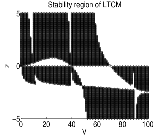
Figure 1: Stability region (shaded area) of the method LTCM.

It is noted that when $M=0$, the method LTCM reduces to a fourth-order RKN method with the Butcher tableau (21) and (30).

In order to show the efficiency and robustness of the fourth-order method, the other integrators we select for comparison are:

• TFCM: a fourth-order trigonometric Fourier collocation method in [19] with $c_{1}=\frac{3-\sqrt{3}}{6},\ c_{2}=\frac{3+\sqrt{3}}{6},\ b_{1}=b_{2}=1/2,\ r=2$;

• SRKM1: the symplectic Runge–Kutta method of order five in [18] based on Radau quadrature;

• EPCM1: the “extended Lobatto IIIA method of order four” in [14], which is an energy-preserving collocation method (the case $s=2$ in [7]);

• EPRKM1: the energy-preserving Runge–Kutta method of order four (formula (19) in [2]).

Since all these methods are implicit, we use the classical waveform Picard algorithm. For each experiment, first we show the convergence rate of iterations for different error tolerances. Then for different methods, we set the error tolerance as $10^{-16}$ and set the maximum number of iteration as 5. We display the global errors and the energy errors if the problem is a Hamiltonian system. The numerical experiments have been carried out on a personal computer and the algorithm has been implemented by using the MATLAB-R2013a.

Problem 1. Consider the Hamiltonian equation which governs the motion of an artificial satellite (this problem has been considered in [17]) with the Hamiltonian

$$H(q,p)=\frac{1}{2}p^{\intercal}p+\frac{1}{2}\frac{\kappa}{2}q^{\intercal}q+\lambda\Big{(}\frac{(q_{1}q_{3}+q_{2}q_{4})^{2}}{r^{4}}-\frac{1}{12r^{2}}\Big{)},$$

where $q=(q_{1},q_{2},q_{3},q_{4})^{\intercal}$ and $r=q^{\intercal}q.$ The initial conditions are given on an elliptic equatorial orbit by

$$q_{0}=\sqrt{\frac{r_{0}}{2}}\Big{(}-1,-\frac{\sqrt{3}}{2},-\frac{1}{2},0\Big{)}^{\intercal},\ \ \ p_{0}=\frac{1}{2}\sqrt{K^{2}\frac{1+e}{2}}\Big{(}1,\frac{\sqrt{3}}{2},\frac{1}{2},0\Big{)}^{\intercal}.$$

Here $M=\frac{\kappa}{2}$ and $\kappa$ is the total energy of the elliptic motion which is defined by $\kappa=\frac{K^{2}-2|p_{0}|^{2}}{r_{0}}-V_{0}$ with $V_{0}=-\frac{\lambda}{12r_{0}^{3}}.$ The parameters of this problem are chosen as $K^{2}=3.98601\times 10^{5}$, $r_{0}=6.8\times 10^{3}$, $e=0.1$, $\lambda=\frac{3}{2}K^{2}J_{2}R^{2},\ J_{2}=1.08625\times 10^{-3},\ R=6.37122\times 10^{3}$. First the problem is solved in the interval $[0,10^{4}]$ with the stepsize $h=\frac{1}{10}$ to show the convergence rate of iterations. See Table 1 for the CPU time of iterations for different error tolerances. Then this equation is integrated in $[0,1000]$ with the stepsizes $1/2^{i}$, $i=2,\cdots,5$. The global errors against CPU time are shown in Fig. 2 (i). We finally integrate this problem with a fixed stepsize $h=1/20$ in the interval $[0,t_{\mathrm{end}}]$ with $t_{\mathrm{end}}=10,100,10^{3},10^{4}$. The maximum global errors of Hamiltonian energy against CPU time are presented in Fig. 2 (ii).

$$\begin{array}[]{|c|c|c|c|c|c|}\hline\cr\text{Methods}&tol=1.0e-006&tol=1.0e-008&tol=1.0e-010&tol=1.0e-012\\ \hline\cr\text{LTCM}&6.8215&8.8964&8.8500&10.5551\cr\text{TFCM}&9.7892&9.7553&9.9806&13.0105\cr\text{SRKM1}&67.0230&64.1777&75.9390&86.8317\cr\text{EPCM1}&104.4341&112.9710&126.4438&145.6188\cr\text{EPRKM1}&56.2409&64.3123&75.2503&84.9962\cr\hline\cr\end{array}$$

Table 1: Results for Problem 1: The total CPU time (s) of iterations for different error tolerances (tol).

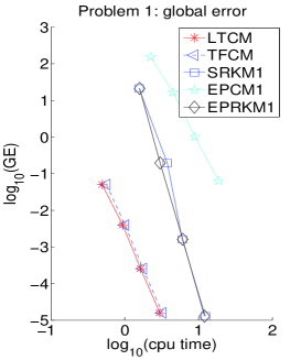
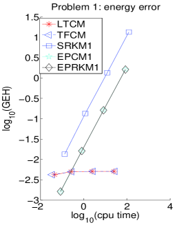
(i)	(ii)

Figure 2: Results for Problem 1. (i): The logarithm of the global error ($GE$) over the integration interval against the logarithm of CPU time. (ii): The logarithm of the maximum global error of Hamiltonian energy ($GEH$) against the logarithm of CPU time.

Problem 2. Consider the Fermi-Pasta-Ulam Problem [9].

Fermi-Pasta-Ulam Problem is a Hamiltonian system with the Hamiltonian

$$\begin{array}[c]{ll}H(y,x)&=\frac{1}{2}\textstyle\sum\limits_{i=1}^{2m}y_{i}^{2}+\frac{\omega^{2}}{2}\textstyle\sum\limits_{i=1}^{m}x_{m+i}^{2}+\frac{1}{4}\Big{[}(x_{1}-x_{m+1})^{4}\\ &+\textstyle\sum\limits_{i=1}^{m-1}(x_{i+1}-x_{m+i-1}-x_{i}-x_{m+i})^{4}+(x_{m}+x_{2m})^{4}\Big{]},\end{array}$$

where $x_{i}$ is a scaled displacement of the $i$th stiff spring, $x_{m+i}$ represents a scaled expansion (or compression) of the $i$th stiff spring, and $y_{i},\ y_{m+i}$ are their velocities (or momenta). This system can be rewritten as

$$x^{\prime\prime}(t)+Mx(t)=-\nabla U(x),\qquad t\in[t_{0},t_{\mathrm{end}}],$$

where

$$M=\left(\begin{array}[c]{cc}\mathbf{0}_{m\times m}&\mathbf{0}_{m\times m}\\ \mathbf{0}_{m\times m}&\omega^{2}I_{m\times m}\end{array}\right),$$

$$U(x)=\frac{1}{4}\Big{[}(x_{1}-x_{m+1})^{4}+\textstyle\sum\limits_{i=1}^{m-1}(x_{i+1}-x_{m+i-1}-x_{i}-x_{m+i})^{4}+(x_{m}+x_{2m})^{4}\Big{]}.$$

Following [9], we choose

$$m=3,\ x_{1}(0)=1,\ y_{1}(0)=1,\ x_{4}(0)=\frac{1}{\omega},\ y_{4}(0)=1$$

with zero for the remaining initial values.

First the problem is solved in the interval $[0,1000]$ with the stepsize $h=\frac{1}{100}$ and $\omega=100,\ 200$ to show the convergence rate of iterations. See Table 2 for the total CPU time of iterations for different error tolerances. It can be observed that when $\omega$ increases, the convergence rate of LTCM and TFCM is almost unaffected. However, the convergence rate of the other methods varies greatly when $\omega$ becomes large.

Then we integrate the system in the interval $[0,50]$ with $\omega=50,100,150,200$ and the stepsizes $h=1/(20\times{2^{j}}),\ j=1,2,3,4.$ The global errors are shown in Fig. 4. Finally we integrate this problem with a fixed stepsize $h=1/100$ in the interval $[0,t_{\mathrm{end}}]$ with $t_{\mathrm{end}}=1,10,100,1000.$ The maximum global errors of Hamiltonian energy are presented in Fig. 4. Here it is noted that some results are too large, thus we do not plot the corresponding points in Figs. 3-4. Similar situation occurs in the next two problems.

$$\begin{array}[]{|c|c|c|c|c|c|}\hline\cr\text{Methods}&tol=1.0e-006&tol=1.0e-008&tol=1.0e-010&tol=1.0e-012\\ \hline\cr\text{LTCM ($\omega=100$)}&7.1570&9.7010&9.6435&12.2449\cr\text{LTCM ($\omega=200$)}&7.5169&10.0160&9.2135&11.1672\cr\hline\cr\text{TFCM ($\omega=100$)}&7.6434&10.3224&10.3341&12.7998\cr\text{TFCM ($\omega=200$)}&7.8861&11.1322&10.0578&12.3621\cr\hline\cr\text{SRKM1 ($\omega=100$)}&32.0491&39.4922&48.5822&57.0720\cr\text{SRKM1 ($\omega=200$)}&58.2410&70.5585&86.1757&99.6403\cr\hline\cr\text{EPCM1 ($\omega=100$)}&50.8899&70.5920&87.9782&102.9839\cr\text{EPCM1 ($\omega=200$)}&121.2714&149.7104&189.4323&220.1096\cr\hline\cr\text{EPRKM1 ($\omega=100$)}&31.0881&39.0050&47.6389&56.4456\cr\text{EPRKM1 ($\omega=200$)}&55.2205&68.8459&82.5919&98.5277\cr\hline\cr\end{array}$$

Table 2: Results for Problem 2: The total CPU time (s) of iterations for different error tolerances (tol).

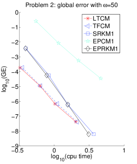
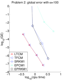
(i)	(ii)
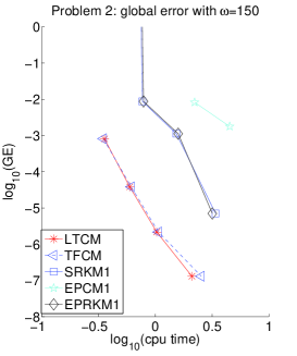
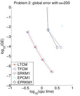
(iii)	(iv)

Figure 3: Results for Problem 2. The logarithm of the global error ($GE$) over the integration interval against the logarithm of CPU time.

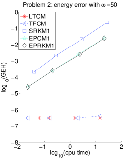
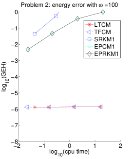
(i)	(ii)
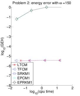
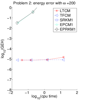
(iii)	(iv)

Figure 4: Results for Problem 2. The logarithm of the maximum global error of Hamiltonian energy ($GEH$) against the logarithm of CPU time.

Problem 3. Consider the nonlinear Klein-Gordon equation [15]

$$\begin{array}[c]{l}\frac{\partial^{2}u}{\partial t^{2}}-\frac{\partial^{2}u}{\partial x^{2}}=-u^{3}-u,\ \ \ 0<x<L,\ \ t>0,\\[8.5359pt] u(x,0)=A(1+\cos(\frac{2\pi}{L}x)),\ \ u_{t}(x,0)=0,\ \ u(0,t)=u(L,t),\end{array}$$

where $L=1.28$, $A=0.9$. Carrying out a semi-discretization on the spatial variable by using second-order symmetric differences yields

$$\begin{array}[]{l}\frac{d^{2}U}{dt^{2}}+MU=F(U),\ \ \ 0<t\leq t_{\mathrm{end}},\\ \end{array}$$

where $U(t)=\big{(}u_{1}(t),\cdots,u_{N}(t)\big{)}^{\intercal}$ with $u_{i}(t)\approx u(x_{i},t),\ i=1,\cdots,N$,

$$M=\frac{1}{\Delta x^{2}}\left(\begin{array}[c]{ccccc}2&-1&&&-1\\ -1&2&-1&&\\ &\ddots&\ddots&\ddots&\\ &&-1&2&-1\\ -1&&&-1&2\\ \end{array}\right)_{N\times N}$$

with $\Delta x=L/N$, $x_{i}=i\Delta x,$ $F(U)=\big{(}-u_{1}^{3}-u_{1},\cdots,-u_{N}^{3}-u_{N}\big{)}^{\intercal}$ and $N=32$. The corresponding Hamiltonian of this system is

$$H(U^{\prime},U)=\frac{1}{2}U^{\prime\intercal}U^{\prime}+\frac{1}{2}U^{\intercal}MU+\frac{1}{2}u^{2}_{1}+\frac{1}{4}u^{4}_{1}+\ldots+\frac{1}{2}u^{2}_{N}+\frac{1}{4}u^{4}_{N}.$$

Here we choose $N=32$. The problem is solved in the interval $[0,500]$ with the stepsize $h=\frac{1}{100}$ to show the convergence rate of iterations. See Table 3 for the total CPU time of iterations for different error tolerances. Then we solve this problem in $[0,20]$ with stepsizes $h=1/(3\times 2^{j}),\ j=1,2,3,4.$ Fig. 5 (i) shows the global errors. Finally this problem is integrated with a fixed stepsize $h=0.002$ in the interval $[0,t_{\mathrm{end}}]$ with $t_{\mathrm{end}}=1,10,100,1000.$ The maximum global errors of Hamiltonian energy are presented in Fig. 5 (ii).

$$\begin{array}[]{|c|c|c|c|c|c|}\hline\cr\text{Methods}&tol=1.0e-006&tol=1.0e-008&tol=1.0e-010&tol=1.0e-012\\ \hline\cr\text{LTCM}&5.9325&7.9263&8.1816&10.0602\cr\text{TFCM}&6.5318&8.7008&8.8934&10.7489\cr\text{SRKM1}&24.1600&29.4173&34.5310&39.5161\cr\text{EPCM1}&37.2757&46.4011&53.1403&66.2339\cr\text{EPRKM1}&22.6571&27.8341&33.5435&39.4533\cr\hline\cr\end{array}$$

Table 3: Results for Problem 3: The total CPU time (s) of iterations for different error tolerances (tol).

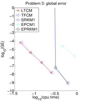
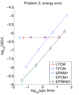
(i)	(ii)

Figure 5: Results for Problem 3. (i): The logarithm of the global error ($GE$) over the integration interval against the logarithm of CPU time. (ii): The logarithm of the maximum global error of Hamiltonian energy ($GEH$) against the logarithm of CPU time.

Problem 4. Consider the wave equation

$$\begin{array}[]{ll}\frac{\partial^{2}u}{\partial t^{2}}-a(x)\frac{\partial^{2}u}{\partial x^{2}}+92u=f(t,x,u),\ \ \ 0<x<1,\ \ t>0,\\ \\ u(0,t)=0,\ \ \ u(1,t)=0,\ \ \ u(x,0)=a(x),\ \ \ u_{t}(x,0)=0,\end{array}$$

with $a(x)=4x(1-x),\ f(t,x,u)=u^{5}-a^{2}(x)u^{3}+\frac{a^{5}(x)}{4}\sin^{2}(20t)\cos(10t).$ The exact solution is $u(x,t)=a(x)\cos(10t).$

Using semi-discretization on the spatial variable with second-order symmetric differences, we obtain

$$\begin{array}[]{ll}\frac{d^{2}U}{dt^{2}}+MU=F(t,U),\ U(0)=\big{(}a(x_{1}),\cdots,a(x_{N-1})\big{)}^{\intercal},\ U^{\prime}(0)={\bf 0},\ 0<t\leq t_{\mathrm{end}},\end{array}$$

where $U(t)=\big{(}u_{1}(t),\ldots,u_{N-1}(t)\big{)}^{\intercal}$ with $u_{i}(t)\approx u(x_{i},t)$, $x_{i}=i\Delta x$, $\Delta x=1/N$, $i=1,\ldots,N-1,$

$$M=92I_{N-1}+\frac{1}{\Delta x^{2}}\left(\begin{array}[c]{ccccc}2a(x_{1})&-a(x_{1})&&&\\ -a(x_{2})&2a(x_{2})&-a(x_{2})&&\\ &\ddots&\ddots&\ddots&\\ &&-a(x_{N-2})&2a(x_{N-2})&-a(x_{N-2})\\ &&&-a(x_{N-1})&2a(x_{N-1})\\ \end{array}\right),$$

and

$$F(t,U)=\big{(}f(t,x_{1},u_{1}),\cdots,f(t,x_{N-1},u_{N-1})\big{)}^{\intercal}.$$

The problem is solved in the interval $[0,100]$ with the stepsize $h=\frac{1}{40}$ to show the convergence rate of iterations. See Table 4 for the total CPU time of iterations for different error tolerances. Then system is integrated in the interval $[0,100]$ with $N=40$ and $h=1/2^{j},\ j=5,6,7,8.$ The global errors are shown in Fig. 6.

It follows from the numerical results that our method LTCM is very promising as compared with the classical methods SRKM1, EPCM1 and EPRKM1. Although LTCM has a similar performance as TFCM in preserving the solution and the energy, it has a better convergence rate of iterations.

$$\begin{array}[]{|c|c|c|c|c|c|}\hline\cr\text{Methods}&tol=1.0e-006&tol=1.0e-008&tol=1.0e-010&tol=1.0e-012\\ \hline\cr\text{LTCM}&1.8980&1.8737&2.1212&2.3196\cr\text{TFCM}&1.9213&1.9345&2.2227&2.3736\cr\text{SRKM1}&13.8634&16.6963&19.0854&22.6142\cr\text{EPCM1}&23.5110&28.1288&32.2263&36.8443\cr\text{EPRKM1}&13.5526&17.2289&18.8744&23.0066\cr\hline\cr\end{array}$$

Table 4: Results for Problem 4: The total CPU time (s) of iterations for different error tolerances (tol).

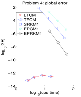
Figure 6: Results for Problem 4: The logarithm of the global error ($GE$) over the integration interval against the logarithm of CPU time.

5 Conclusions and discussions

In this paper we have investigated a kind of trigonometric collocation methods based on Lagrange basis polynomials, the variation-of-constants formula and the idea of collocation methods for solving multi-frequency oscillatory second-order differential equations (1) efficiently. It has been shown that the convergent condition of these trigonometric collocation methods is independent of $\left\|M\right\|$, which is very important and crucial for solving highly oscillatory systems. The numerical experiments with some model problems show that the our method derived in this paper has remarkable efficiency in comparison with some existing methods in the literature.

References

[1] L. Brugnano, F. Iavernaro, Line Integral Methods for Conservative
Problems, CRC Press, Boca Raton (FL), 2016.
[2] L. Brugnano, F. Iavernaro, D. Trigiante, A simple framework for the derivation and analysis of effective
one-step methods for ODEs, Appl. Math. Comput. 218 (2012)
8475–8485.
[3] D. Cohen, Conservation properties of numerical integrators for highly
oscillatory Hamiltonian systems, IMA J. Numer. Anal. 26 (2006)
34–59.
[4]
D. Cohen, E. Hairer, C. Lubich, Numerical Energy Conservation for
Multi-Frequency Oscillatory Differential Equations, BIT 45 (2005)
287–305.
[5] D. Cohen, T. Jahnke, K. Lorenz, C. Lubich, Numerical
integrators for highly oscillatory Hamiltonian systems: a review, in
Analysis, Modeling and Simulation of Multiscale Problems (A. Mielke,
ed.), Springer, Berlin, (2006) 553–576.
[6]
B. García-Archilla, J. M. Sanz-Serna, R. D.Skeel,
Long-time-step methods for oscillatory differential equations, SIAM
J. Sci. Comput. 20 (1999) 930–963.
[7] E. Hairer,
Energy-preserving variant of collocation methods, JNAIAM J.
Numer. Anal. Ind. Appl. Math. 5 (2010) 73–84.
[8]
E. Hairer, C. Lubich,
Long-time energy
conservation of numerical methods for oscillatory differential
equations, SIAM J. Numer. Anal. 38 (2000) 414–441.
[9]
E. Hairer, C. Lubich, G. Wanner,
Geometric
Numerical Integration: Structure-Preserving Algorithms for Ordinary
Differential Equations, 2nd ed., Springer-Verlag, Berlin,
Heidelberg, 2006.
[10] J.K. Hale, Ordinary Differential Equations,
Roberte E. Krieger Publishing company, Huntington, New York, 1980.
[11]
M. Hochbruck, C. Lubich, A Gautschi-type method for oscillatory
second-order differential equations, Numer. Math. 83 (1999)
403–426.
[12] M. Hochbruck, A. Ostermann, Explicit
exponential Runge-Kutta methods for semilineal parabolic problems,
SIAM J. Numer. Anal. 43 (2005) 1069-1090.
[13] M. Hochbruck, A. Ostermann, J.
Schweitzer, Exponential Rosenbrock-type methods, SIAM J. Numer.
Anal. 47 (2009) 786-803.
[14] F. Iavernaro, D. Trigiante,
High-order symmetric schemes for the energy conservation of
polynomial Hamiltonian problems, JNAIAM J. Numer. Anal. Ind. Appl.
Math. 4 (1) 2009.
[15]
S. Jiménez, L. Vázquez, Analysis of four numerical schemes
for a nonlinear Klein-Gordon equation, Appl. Math. Comput.
35 (1990) 61–93.
[17] E.L. Stiefel, G. Scheifele, Linear and regular celestial mechanics, Springer-Verlag, New York,
1971.
[18] Sun Geng, Construction of high order symplectic Runge–Kutta methods,
J. Comput. Math. 11 (1993) 250–260.
[19] B. Wang, A. Iserles, X. Wu, Arbitrary–order trigonometric Fourier collocation methods for
multi-frequency oscillatory systems, Found. Comput. Math. 16
(2016) 151-181.
[20] B. Wang, G. Li,
Bounds on asymptotic-numerical solvers for ordinary differential
equations with extrinsic oscillation, Appl. Math. Modell.
39 (2015) 2528-2538.
[21] B. Wang, K. Liu, X. Wu,
A Filon-type asymptotic approach to solving highly oscillatory
second-order initial value problems, J. Comput. Phys. 243 (2013)
210-223.
[22] B. Wang, X. Wu, A new high precision
energy-preserving integrator for system of oscillatory second-order
differential equations, Phys. Lett. A 376 (2012) 1185–1190.
[23]
B. Wang, X. Wu, H. Zhao, Novel improved multidimensional Störmer-Verlet formulas with
applications to four aspects in scientific computation, Math.
Comput. Modell. 57 (2013) 857–872.
[24] B. Wang, X. Wu, J. Xia, Error bounds for explicit ERKN integrators for systems of multi-frequency oscillatory second-order
differential equations, Appl. Numer. Math. 74 (2013) 17–34.
[25] X. Wu, A note on stability of multidimensional
adapted Runge-Kutta-Nyström methods for oscillatory systems,
Appl. Math. Modell. 36 (2012) 6331–6337.
[26]X. Wu, B. Wang, W. Shi, Efficient energy-preserving integrators for
oscillatory Hamiltonian systems, J. Comput. Phys. 235 (2013)
587–605.
[27] X. Wu, B. Wang, J. Xia, Explicit symplectic
multidimensional exponential fitting modified
Runge-Kutta-Nyström methods, BIT 52 (2012) 773–795.
[28] X. Wu, X. You, W. Shi, B. Wang, ERKN
integrators for systems of oscillatory second-order differential
equations, Comput. Phys. Comm. 181 (2010) 1873–1887.
[29] X. Wu, X. You, B. Wang, Structure-Preserving Algorithms for Oscillatory
Differential Equations, Springer-Verlag, Berlin, Heidelberg, 2013.