Improving the Flux Calibration in Reverberation Mapping by Spectral Fitting: Application to the Seyfert Galaxy MCG–6-30-15

Abstract

We propose a method for the flux calibration of reverberation mapping spectra based on accurate measurement of [O iii] $\lambda 5007$ emission by spectral fitting. The method can achieve better accuracy than the traditional method of van Groningen & Wanders (1992), allowing reverberation mapping measurements for object with variability amplitudes as low as $\sim$ 5%. As a demonstration, we reanalyze the data of the Seyfert 1 galaxy MCG–6-30-15 taken from the 2008 campaign of the Lick AGN Monitoring Project, which previously failed to obtain a time lag for this weakly variable object owing to a relatively large flux calibration uncertainty. We detect a statistically significant rest-frame time lag of $6.38_{-2.69}^{+3.07}$ days between the H$\beta$ and $V$-band light curves. Combining this lag with FWHM(H$\beta$) = $1933\pm 81$ $\rm km~{}s^{-1}$ and a virial coefficient of $f$ = 0.7, we derive a virial black hole mass of $3.26_{-1.40}^{+1.59}\times 10^{6}$ $M_{\odot}$, which agrees well with previous estimates by other methods.

1. Introduction

Reverberation mapping (Blandford & McKee, 1982) is the most widely applied method for measuring black hole masses in active galactic nuclei (AGNs) (see Peterson 2014 for a review). It employs spectroscopic monitoring to derive the mass from the dynamics of the broad-line region (BLR) clouds that orbit in the gravitational potential of the black hole. The emission-line width provides an estimate of the cloud velocity, while the time lag between the continuum and emission line (usually H$\beta$) variability, caused by the light-travel time between the central continuum and the clouds, yields the BLR size. Thus, accurate flux calibration is essential for lag measurement in reverberation mapping. The most widely used method is the spectral scaling algorithm of van Groningen & Wanders (1992, hereinafter vGW92), based on the normalization of the [O iii] $\lambda$5007 emission-line intensity, which is assumed to be constant over the timescale of monitoring observations (Peterson et al., 2013). The uncertainty in flux calibration achieved by this method can be as large as $\sim$ 3% (Barth et al., 2015). This level of uncertainty may lead to erroneous interpretation of AGN light curves for objects with weak variability, as shown by Barth & Bentz (2016) for Mrk 142, whose variabilities in the $B$ and $V$ bands are $\lesssim$ 3% Walsh et al. (2009). New methods for flux calibration in reverberation mapping observations would be valuable.

The spectral fitting method has been used for emission-line measurements in several reverberation mapping studies (e.g., Park et al., 2012; Barth et al., 2013, 2015; Hu et al., 2015), and it has proved to be an improvement in these cases to the traditional integration method. By measuring the flux of the [O iii] emission line, spectral fitting also naturally can be used for flux calibration, with the potential to achieve higher accuracy than the “standard” method of vGW92. However, spectral fitting has not been adopted yet for flux calibration in previous reverberation studies; Park et al. (2012) and Barth et al. (2013, 2015) still used the method of vGW92 for flux calibration, while Hu et al. (2015) used a flux calibration strategy that does not rely on the [O iii] emission line but on simultaneous observations of a comparison star. It is worth revisiting reverberation mapping observations that previously had poor flux calibration, to test whether spectral fitting can offer any improvement.

MCG–6-30-15 is a well-studied nearby ($z$ = 0.008) Seyfert 1 galaxy (e.g., Reynolds et al., 1997; McHardy et al., 2005; Marinucci et al., 2014; Lira et al., 2015, and references therein), famous for its broad iron K$\alpha$ line (e.g., Tanaka et al., 1995; Fabian et al., 2002; Miniutti et al., 2007; Marinucci et al., 2014). The mass of the black hole in MCG–6-30-15 has been estimated by many methods (McHardy et al., 2005, and references therein), all but reverberation mapping. MCG–6-30-15 was spectroscopically monitored in the optical by the Lick AGN Monitoring Project (LAMP) in 2008 (Bentz et al., 2009). This object is very difficult to observe from Lick Observatory due to its southern declination; the median air mass was 3.2 throughout the campaign (Bentz et al., 2009). In addition, the variability of this object during the entire observing period was rather weak ($\lesssim$ 4% in the $B$ and $V$ bands; Walsh et al. 2009), putting greater demands on very accurate spectroscopic flux calibration. Bentz et al. (2009) adopted the method of vGW92, which apparently is not good enough for this object; no BLR time lag was detected because of its noisy H$\beta$ light curve.

Here, we revisit the LAMP 2008 data of MCG–6-30-15, show that both the flux calibration and emission-line measurement can be improved by spectral fitting, successfully detect the time lag of the H$\beta$ emission line relative to the AGN continuum, and derive the mass of the central black hole of this important source. In Appendix A, we also analyze archival Hubble Space Telescope (HST) Wide Field Camera 3 (WFC3) images of MCG–6-30-15, determine its bulge classification, and derive the starlight contribution to the spectroscopic flux.

2. Flux Calibration

The details of the observations and data reductions of LAMP 2008 were presented by Walsh et al. (2009) and Bentz et al. (2009). The photometric monitoring of MCG–6-30-15 included 48 epochs of $B$-band observations with a median cadence of 1.08 days and 55 epochs of $V$-band data with a median cadence of 1.04 days. The spectroscopy covered 42 epochs with a median cadence of 1.00 days. LAMP 2008 publicly released two sets of spectra: one flux calibrated in the usual manner using standard stars, and another by scaling to a common flux for the narrow [O iii] $\lambda$5007 line, following the procedure of vGW92. Because of variable sky transparency and slit losses due to seeing and mis-centering, standard flux calibration is usually not accurate enough for reverberation mapping. Further refinement in the calibration can be accomplished by noting that the flux of [O iii] should be constant over the timescales of the experiment (Peterson et al., 2013). The H$\beta$ light curves in Bentz et al. (2009) were obtained from the scaled spectra, but the line fluxes were measured by simple integration of the line after subtraction of a linear, locally defined continuum.

For comparison, we repeat the measurement of the H$\beta$ light curve of MCG–6-30-15 in Bentz et al. (2009), using the scaled spectra with the same continuum and line windows. Our results, shown in the top panel of Figure 1, agree well with those in Bentz et al. (2009). Note that the error bars here account only for measurement errors, whereas the much larger values in Figure 3 of Bentz et al. (2009) include systematic errors in the light curve. We show below that this systematic error can be reduced.

Figure 1.— Light curves of H$\beta$ (top) and [O iii] (bottom) measured from the scaled spectra by simple integration, as in Bentz et al. (2009), but without plotting the systematic error. The scatter in the [O iii] light curve ($\sim$3%) represents the flux calibration accuracy of the scaled spectra.

2.1. Flux Calibration Accuracy of the Scaled Spectra

As the final, calibrated spectra are expected to have the same [O iii] flux, the scatter in the [O iii] flux can be used to estimate the accuracy of the flux calibration. The bottom panel of Figure 1 shows the [O iii] light curve measured by integrating the flux above the continuum in the wavelength range 5030–5065 Å, using the same continuum windows as for H$\beta$. The scatter in [O iii] flux is $\sim$3%. This accuracy is comparable to that normally achieved in other reverberation mapping observations, $\sim$2% (e.g., Peterson et al., 1998a; Kaspi et al., 2000). However, the scatter in H$\beta$ for this object is only $\sim$7%. Moreover, the two light curves are apparently correlated; their cross-correlation function (CCF) has a peak value $r_{\rm max}$ $\approx$ 0.7. The scaled spectra are not calibrated accurately enough for studying the variability of H$\beta$ flux in this object.

The spectral scaling algorithm of vGW92 does not depend on the measurement of the narrow-line flux, in order to avoid the uncertainty in the determination of the continuum, which is significant when the continuum is defined as a simple straight line set between two wavelength windows. Hu et al. (2015) illustrate that spectral fitting enables the continuum to be properly defined and line fluxes to be accurately measured. Thus, we recalibrate the reduced spectra by scaling to the [O iii] flux measured from an initial spectral fitting. Then, we perform a second, more refined fitting on the recalibrated spectra to measure the light curves. Before the initial fitting, we correct the reduced spectra for Galactic extinction using the $R_{V}$-dependent law of Cardelli et al. (1989) and O’Donnell (1994). We assume $R_{V}$ = 3.1 and adopt the $V$-band extinction of 0.165 mag from the NASA/IPAC Extragalactic Database. All the spectra and light curves hereafter are plotted after correcting for Galactic extinction.

2.2. Recalibration of the Reduced Spectra

Due to signal-to-noise ratio (S/N) considerations, Hu et al. (2015) fitted each individual spectrum by fixing the values of some parameters to those obtained from the best fit to the mean spectrum. The fixed parameters include the spectral index of the power-law continuum, the velocity width and shift of the broad He ii line, and the strength of narrow emission lines. As the mean spectrum will not be calculated before the recalibration, here we omit the broad He ii and weak narrow lines from the preliminary fit, only including a single power-law continuum, the host galaxy, Fe ii emission, broad and narrow H$\beta$, and [O iii] $\lambda\lambda$4959, 5007. Accordingly, the preliminary fit is performed in relatively narrow wavelength windows, covering rest-frame 4430–4600 and 4750–5550 Å (see hatched regions in Fig. 2). The narrow H$\beta$ line is constrained to have the same width and shift as [O iii], while all the other parameters are set free. As shown in Section 3, this preliminary fitting yields [O iii] fluxes accurate enough for the purpose of flux calibration.

Then, for each reduced spectrum, a scaling factor is calculated by dividing a fiducial flux of $1.02\times 10^{-13}$ erg s^-1 cm^-2 (obtained from the [O iii] $\lambda$5007 flux of $0.856\times 10^{-13}$ erg s^-1 cm^-2 listed in Table 3 of Bentz et al. 2009 after correcting for Galactic extinction) by our measured [O iii] flux. By simple scaling of this factor, we obtain recalibrated spectra for the following light curve measurements and analysis.

3. Light Curve Measurements and Analysis

Following Hu et al. (2015), we generate light curves from the best-fit values of the corresponding parameters obtained from the second, more refined spectral fitting of the recalibrated spectra. Figure 2 shows an example of the fit. Compared to the preliminary fitting in Section 2.2, broad and narrow He ii $\lambda$4686 and several narrow coronal lines are added, and some parameters are fixed to their values obtained from the best fit to the mean spectrum. Note that the apparent flux variation of the host galaxy described in Appendix A of Hu et al. (2015) also exists here, because the size of the [O iii]-emitting region is different from that of the host galaxy. This is evident from the absorption features in the root-mean-square (rms) spectrum in Figure 6 of Bentz et al. (2009). Thus, as in Hu et al. (2015), the fit allows the flux of the host galaxy to vary. In total, there are 16 free parameters, along with 13 others fixed. We remove from the analysis seven spectra with S/N $<$ 40 (calculated around rest-frame wavelength 5100 Å) and another four with reduced $\chi^{2}$ $>$ 2.4.

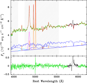
Figure 2.— Sample fit of a recalibrated spectrum. Pixels included in the fit are plotted in green, whereas excluded pixels are in black. The best-fit model (red) is composed of the AGN power-law continuum (blue), Fe ii emission (blue; template from Boroson & Green 1992), host galaxy (blue; template with 11 Gyr age and metallicity $Z$ = 0.05 from Bruzual & Charlot 2003), broad H$\beta$ (magenta), broad He ii $\lambda$4686 (cyan), and several narrow emission lines (orange). The bottom panel shows the residuals. The hatched regions show the wavelength windows in the preliminary fitting for the flux calibration.

The only difference between the procedure here and that of Hu et al. (2015) is that we now include narrow H$\beta$ in the fit, because it can be decomposed well in the mean spectrum. For each individual-night spectrum, we constrain the velocity width and shift of narrow H$\beta$ to be the same as those of [O iii], and we fix the intensity ratio of narrow H$\beta$ to [O iii] $\lambda$5007 to 0.13, as given by the best-fit mean spectrum. This intensity ratio is consistent with that measured by Reynolds et al. (1997) from their nuclear spectrum of MCG–6-30-15. For each individual-night spectrum, both the FWHM and the dispersion ($\sigma$) of broad H$\beta$ are calculated from the best-fit Gauss-Hermite model; their mean and standard deviation are used as the measurement of the broad H$\beta$ width and its associated uncertainty. After correcting an instrument broadening of 12.5 Å given by Bentz et al. (2009), we obtain FWHM = 1933 $\pm$ 81 $\rm km~{}s^{-1}$ and $\sigma$ = 1175 $\pm$ 78 $\rm km~{}s^{-1}$. As a consistency check, we also analyzed archival HST Space Telescope Imaging Spectrograph (STIS) spectra of MCG–6-30-15, in which the broad and narrow H$\beta$ components are clearly separated (see Fig. 13 of McHardy et al. 2005). The FWHM and $\sigma$ of the broad H$\beta$ from the STIS spectra are $1935\pm 17$ and $1152\pm 10$ $\rm km~{}s^{-1}$, respectively, in good agreement with the measurements obtained above. This demonstrates the robustness of our spectral decomposition and correction for instrument broadening.

Table 1Measured and Derived Properties of MCG–6-30-15

Parameter	Value
FWHM (H$\beta$)	1933 $\pm$ 81 $\rm km~{}s^{-1}$
$\sigma$ (H$\beta$)	1175 $\pm$ 78 $\rm km~{}s^{-1}$
$F_{\rm var}$ (H$\beta$)	5.3 $\pm$ 1.1 %
$r_{\rm max}$ (H$\beta$ vs. $V$)	0.55
$\tau$ (H$\beta$ vs. $V$)	$6.38_{-2.69}^{+3.07}$ days
$c\tau{\rm FWHM}^{2}/G$	$4.66_{-2.00}^{+2.28}\times 10^{6}$ $M_{\odot}$
$c\tau\sigma^{2}/G$	$1.72_{-0.76}^{+0.86}\times 10^{6}$ $M_{\odot}$
$M_{\bullet}$ (FWHM, $f=0.7$)	$3.26_{-1.40}^{+1.59}\times 10^{6}$ $M_{\odot}$
$M_{\bullet}$ ($\sigma$, $f=3.2$)	$5.51_{-2.43}^{+2.75}\times 10^{6}$ $M_{\odot}$

The scatter of the measured [O iii] flux (bottom panel of Fig. 3) is only $\sim$0.5%, which is less than the fitting error; this indicates that our recalibration successfully achieved its goal, and that there is no need to scale further. The light curve of H$\beta$ is shown in the lower-middle panel. The error bars of the H$\beta$ flux include both the fitting error and a systematic error estimated from the scatter in the measured fluxes of successive nights. The variability amplitude $F_{\rm var}$ (Rodríguez-Pascual et al., 1997; Edelson et al., 2002) of H$\beta$ is 5.3 $\pm$ 1.1 %. The top and upper-middle panels show the $B$-band and $V$-band photometric light curves of Walsh et al. (2009). As in Bentz et al. (2009), we use the photometric light curves as the continuum light curve in the time-series analysis; the light curve of the power-law flux density derived from the spectral fit has large scatter.

Figure 3.— Light curves in the $B$ and $V$ bands (top and upper-middle; from Walsh et al. 2009), broad H$\beta$ (lower-middle), and [O iii] (bottom). Note the significant improvement in our flux calibration, shown by the much smaller scatter in the [O iii] flux here, as compared to Figure 1.

We calculate the CCF using the interpolation cross-correlation function method (Gaskell & Sparke, 1986; Gaskell & Peterson, 1987; White & Peterson, 1994), adopting the centroid above 80% of the peak value ($r_{\rm max}$) as the time lag (Koratkar & Gaskell, 1991; Peterson et al., 2004). Following Maoz & Netzer (1989) and Peterson et al. (1998b), the CCF calculation is repeated for 5000 Monte Carlo realizations, in each of which a random subset of data points is selected and the fluxes are modified by random Gaussian deviates based on their errors. The 15.87% and 84.13% quantile of the yielded cross-correlation centroid distribution (CCCD) are used as the lower and upper uncertainty bounds of the time lag. Figure 4 shows the CCFs (black solid lines) for H$\beta$ with respect to the $B$ (top) and $V$ (bottom) bands and the corresponding CCCDs (blue histograms). The rest-frame time lag between H$\beta$ and the $V$-band continuum is $\tau=6.38_{-2.69}^{+3.07}$ days, with $r_{\rm max}$ = 0.55. The CCF with respect to the $B$ band gives a consistent time lag but with large uncertainty ($\tau=4.45_{-2.49}^{+9.44}$ days), as a consequence of the large scatter in the $B$-band light curve. Note that the time lag between H$\beta$ and the broad-band continuum is expected to be different from that between H$\beta$ and the AGN continuum at 5100 Å, for two reasons. First, in a thin accretion disk different radii emit continuum radiation peaked at different wavelengths, as a result of which the lag varies with wavelength as $\tau\propto\lambda^{4/3}$ (Collier et al. 1998). Second, the broad-band light curves are contaminated by broad-emission lines. Of the two bands, $V$ has a pivot wavelength closer to 5100 Å but is more contaminated by line emission. Both effects have been reported previously. For example, Fausnaugh et al. (2016) found a lag of $\sim 0.6$ days between the $B$-band and $V$-band light curves of NGC 5548, and effect attributable to the contamination of the continuum bands by broad emission lines; this affects the inferred broad-band lag by $\sim 0.6-1.2$ days. In the case of MCG–6-30-15, which has a smaller black hole mass and lower luminosity, such systematic effects are expected to be smaller than in NGC 5548 and cannot be distinguished given the much larger uncertainties in the measured time lags. The following discussion adopts the time lag with respect to the $V$ band, because the variation in the $V$ band is stronger than that in the $B$ band and gives a time lag with smaller uncertainty. (Note that for the other objects in LAMP 2008 the $B$-band light curve typically has stronger variation and thus was used to determine the time lag in Bentz et al. 2010.)

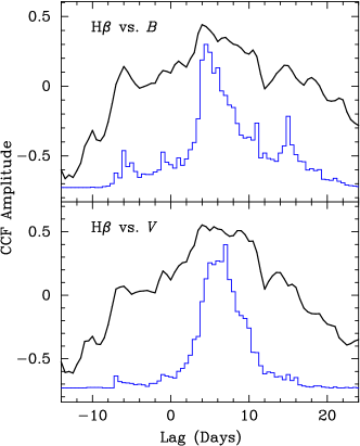
Figure 4.— Cross-correlation functions (black solid lines) for H$\beta$ with respect to the $B$ (top) and $V$ (bottom) band. The blue histogram in each panel is the cross-correlation centroid distribution, which represents the error of the time lag.

Reverberation mapping observations of H$\beta$ have established an empirical relation between the BLR radius and luminosity ($R_{\rm BLR}$–$L$) (e.g., Kaspi et al., 2000; Bentz et al., 2013; Du et al., 2015). Subtracting the starlight contribution based on the HST WFC3 images of MCG–6-30-15 (Appendix A) yields an AGN flux density at 5100 Å of $\sim 1.1\times 10^{-15}$ erg s^-1 cm^-2 Å^-1. For a luminosity distance of 33 Mpc, we obtain a spectral luminosity of $\lambda L_{\lambda}$(5100 Å) $\approx 7.1\times 10^{41}$ erg s^-1, which, from the $R_{\rm BLR}$–$L$ relation of Bentz et al. (2013), predicts $R_{\rm BLR}\approx 2.4$ lt-days. The Balmer decrement and color of the power-law continuum suggest that MCG–6-30-15 may be heavily dust reddened. Adopting a reddening of $E(B-V)=0.61$ mag (Reynolds et al., 1997) yields a much higher intrinsic luminosity of $\lambda L_{\lambda}$(5100 Å) $\approx 4.9\times 10^{42}$ erg s^-1 and $R_{\rm BLR}\approx 6.7$ lt-days. Considering the uncertainties in both the time lag and reddening, our results show no evidence that MCG–6-30-15 deviates from the $R_{\rm BLR}$–$L$ relation.

4. Discussion

4.1. Mean and rms Spectra

In reverberation mapping studies, mean and rms spectra are generated for measuring the emission-line width. The rms spectrum is preferred for representing the variable part of the emission line (Peterson et al. 2004; but see Barth et al. 2015 for biases). However, as mentioned in Section 3, the rms spectrum of MCG–6-30-15 shows H$\beta$ absorption instead of emission because the apparent spectral variability is dominated by variations in the level of host galaxy contamination. Here, following Barth et al. (2015), we produce two sets of mean and rms spectra, an original set generated in the standard manner and another generated after subtracting the best-fit AGN power-law continuum and host galaxy component from each individual spectrum.

Because only a scaling factor was applied to the reduced spectra (see Section 2.2), our recalibrated spectra still suffer from small nightly offsets in wavelength shift and spectral resolution. Skipping the corrections for these offsets does not influence our measurements afterwards because the widths and shifts of both H$\beta$ and [O iii] are free to vary in our fitting; it conveniently allows us calculate the error of the recalibrated spectrum. However, the rms spectrum around strong narrow emission lines (e.g., [O iii]) is strongly affected by these nightly offsets. Thus, before generating the mean and rms spectra, we correct the offsets by applying a linear wavelength shift and a Gaussian broadening to each individual spectrum according to the [O iii] velocity shift and width measured in our preliminary fitting used for recalibration.

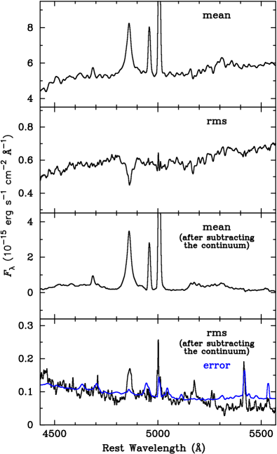
Figure 5.— Mean and rms spectra generated in the standard manner (top and upper-middle) and after subtracting the best-fit AGN power-law continuum and host galaxy component from each individual spectrum (lower-middle and bottom). The blue curve in the bottom panel is the mean of the error in individual spectrum, which would be the rms spectrum if the object is non-varying.

Figure 5 shows the two sets of mean and rms spectra. The standard rms spectrum (upper-middle panel) resembles that presented in Figure 6 of Bentz et al. (2009). It shows no H$\beta$ emission but absorption, because the variability of the H$\beta$ line is overwhelmed by the variations in the AGN power-law continuum and the level of host galaxy contamination. After subtracting the best-fit continuum components, which includes both the AGN power-law and the host galaxy from each individual spectrum, the resulting rms spectrum (black curve in the bottom panel) has much lower intensity than the original one, and shows emission features of H$\beta$ and [O iii]. The blue curve in the bottom panel is the mean of the errors of individual-night spectra in each wavelength bin, which represents the minimal level of rms variations that could be generated. It is the expected rms spectrum of a non-varying object, for which the variations in the observed spectra are totally caused by the observational errors. By comparing the continuum-subtracted rms spectrum and the error spectrum, the apparent variation of the [O iii] line can be mostly attributed to observational error; it also illustrates that our recalibration works well. On the other hand, the H$\beta$ line revealed in the continuum-subtracted rms spectrum is much stronger than the error, which means that the variability of the H$\beta$ line is observable and successfully measured by our spectral fitting. Fitting a single Gaussian with a local continuum to the H$\beta$ line in the continuum-subtracted rms spectrum yields a FWHM of 1104 $\rm km~{}s^{-1}$ (after instrumental broadening correction), which is much narrower than the mean FWHM of the individual spectrum listed in Table 1, a possible consequence of biases due to the weak variability of the feature (see Barth et al. 2015 for detailed discussions).

4.2. Black Hole Mass

Combining the time lag $\tau$ with the emission-line width $\Delta V$ provides an estimate of the virial mass of the black hole,

$$M_{\bullet}=f\frac{c\tau\Delta V^{2}}{G}~{},$$ (1)

where $c$ is the speed of light, $G$ is the gravitational constant, and $f$ is a virial factor that absorbs the unknown geometry, kinematics, and orientation of the BLR. As shown above, the usual way of measuring $\Delta V$ from the rms spectrum is not suitable for MCG–6-30-15 here. The continuum-subtracted rms spectrum does reveal the variation of the H$\beta$ emission line but may still be biased for broad-line width measurement due to the noise in each individual spectrum (see the simulations in Barth et al. 2015). Thus, we measure FWHM and $\sigma$ from the best-fit model of each individual spectrum, and we compute $\Delta V$ from the mean of the individual measurements over the entire observing campaign. In practice (e.g., Onken et al., 2004), the $f$-factor is calibrated from the $M_{\bullet}$–$\sigma_{\ast}$ relation of inactive galaxies (see Kormendy & Ho 2013 for review), which depends on bulge type, being systematically lower for pseudobulges than classical bulges (Ho & Kim, 2014). With a bulge-to-total light ratio of 0.06 and a bulge Sérsic of $n$ = 1.29 (derived from archival HST WFC3 images; Appendix A), MCG–6-30-15 appears to host a pseudobulge. Adopting $f$ = 0.7 (Ho & Kim, 2014) for $\Delta V$ = FWHM, we estimate $M_{\bullet}$ = $3.26_{-1.40}^{+1.59}\times 10^{6}$ $M_{\odot}$; with $\Delta V=\sigma$, $f$ = 3.2 and $M_{\bullet}$ = $5.51_{-2.43}^{+2.75}\times 10^{6}$ $M_{\odot}$. Table 1 lists all measured and derived quantities for MCG–6-30-15.

The black hole mass in MCG–6-30-15 previously has been estimated using a variety of methods, with that from the X-ray power-spectral density technique yielding smallest uncertainty: $2.9_{-1.6}^{+1.8}\times 10^{6}$ $M_{\odot}$ (McHardy et al. 2005). Other estimates, including those from the correlations between black hole mass and bulge properties and photoionization-based calculations of the BLR size, all employed optical observations and derived values between in the range $\sim(3-6)\times 10^{6}$ $M_{\odot}$ (see the comprehensive discussion in McHardy et al. 2005). All these methods are indirect, based on correlations between certain observables and the black hole mass. This work is the first successful direct measurement of the black hole mass in MCG–6-30-15, based on the dynamics of gas in the gravitational potential of the black hole itself. Our two measurements, based on FWHM and $\sigma$, are both in the range of masses given by previous studies, but have smaller uncertainties. We prefer the mass based on FWHM ($3.26_{-1.40}^{+1.59}\times 10^{6}$ $M_{\odot}$) because it is in better agreement with the mass estimate from X-ray variability.

MCG–6-30-15 has an H$\beta$ line width (FWHM $<$ 2000 $\rm km~{}s^{-1}$) that formally qualifies it as a narrow-line Seyfert 1 galaxy (Osterbrock & Pogge, 1985), although its Fe ii emission is not as strong and the [O iii]/H$\beta$ ratio is not as low as in most objects of this class. For a canonical bolometric correction of $L_{\rm bol}=9.8L_{5100}$ (McLure & Dunlop, 2004), we obtain an Eddington ratio of $L_{\rm bol}/L_{\rm Edd}$ = 0.12 using the virial black hole mass based on the H$\beta$ FWHM and the intrinsic luminosity assuming a reddening of $E(B-V)=0.61$ mag. Such an Eddington ratio is low among narrow-line Seyfert 1 galaxies (see, e.g., Figure 1 of Xu et al. 2012), but consistent with the weak Fe ii emission in this object.

4.3. Remarks on the Calibration and Measurement Methods

The spectral scaling algorithm of vGW92 is the most widely used method for flux calibration of reverberation mapping observations. It has proven to be effective in most cases. However, as mentioned in Barth et al. (2015) and shown in Figure 1 of this paper, the uncertainty in the flux calibration achieved can be as large as $\sim$3%. This is not accurate enough for studying objects with weak variability, such as MCG–6-30-15. Barth et al. (2015) also find that the vGW92 method does not work optimally for the objects with low [O iii] equivalent width. Moreover, [O iii] $\lambda$5007 is blended with Fe ii $\lambda$5018, which may be strong and variable (Hu et al. 2015; see their Fig. 3 for examples); under these circumstances, spectral decomposition is necessary to deblend [O iii]. This paper demonstrates that spectral fitting provides a reliable and straightforward way to measure robust [O iii] line strengths, which improves the flux calibration accuracy to $\sim$0.5%.

The spectral fitting method has been used more and more to measure light curves in recent reverberation mapping studies (e.g., Bian et al., 2010; Barth et al., 2013, 2015; Hu et al., 2015). This method is useful for dealing with blended emission lines such as Fe ii and He ii, and it can also improve the measurement of H$\beta$ (see Fig. 6 of Hu et al. 2015 for a comparison with the traditional integration method). For objects with strong host galaxy contribution, spectral fitting also allows correction for the apparent flux variation of the host galaxy (Hu et al., 2015), thereby reducing the contamination of H$\beta$ emission by absorption, as in the case of MCG–6-30-15 here.

In summary, our success in obtaining a time lag measurement for MCG–6-30-15 in this paper results from improvements in both flux calibration and light curve measurements. This is accomplished by spectral fitting in two steps: an initial fit to obtain the [O iii] flux for calibration, followed by a second fit to include additional spectral components to extract the light curve of the broad H$\beta$ emission line. We have demonstrated for the first time the power of this technique in flux calibration, and suggest applying it as an alternative approach in future reverberation studies, especially those of objects with weak variability.

Appendix A Host Galaxy

The host galaxy of MCG–6-30-15 is classified as an S0 galaxy by Malkan et al. (1998), based on HST Wide Field and Planetary Camera 2 images that show a saturated nucleus and a dust lane on one side of major axis. In this Appendix, we analyze archival HST/WFC3 images of this galaxy (GO-11662, PI: Bentz), for two purposes: (1) determining the bulge classification and (2) measuring the starlight flux contribution to the spectroscopic flux at 5100 Å.

MCG–6-30-15 was observed by the WFC3 Ultraviolet-Visible (UVIS) channel with the F547M filter (see Bentz et al. 2013 for the details of the observations). Two sets of exposures with integration times of 25, 370, and 750 s were taken. We retrieve the flat-fielded images of the six exposures from the HST archives and replaced the saturated pixels in the long-exposure images with scaled versions of unsaturated pixels from the shallower exposures. Then, we use the DrizzlePac task AstroDrizzle (version 1.1.16; Gonzaga et al. 2012) to clean cosmic rays, correct geometric distortion, and create the final combined image (Figure 6a) and error image. We generate point-spread function (PSF) models using Tiny Tim (version 7.5; Krist et al. 2011) for each exposure, and combine them in the same way as the galaxy images.

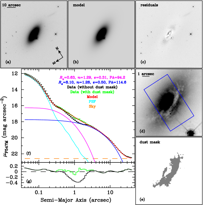
Figure 6.— (a)–(c) HST WFC3 F547M image, best-fit model, and residuals for MCG–6-30-15. Panel (d) zooms in around the nucleus to show the dust lane and spectroscopic extraction aperture (blue rectangle). (e) The final converged dust mask (see text for details). (f) One-dimensional surface brightness profile (black points with error bars), the best-fit model (red line), and the individual component for the bulge (magenta line) and disk (blue line). The PSF is shown as a cyan line. (g) The residuals between the data (with and without the dust mask) and the model.

We use GALFIT (version 3.0.5; Peng et al. 2002, 2010) to perform two-dimensional surface brightness decomposition. The model includes the following components: (1) two PSF profiles for the AGN and the nearby bright star to the south, (2) two Sérsic (1968) profiles for the bulge and disk of the host galaxy, and (3) a constant background sky. A dust mask is needed for the central dust lane (Figure 6d). We generate it iteratively. We first fit the image without a dust mask and generate an initial mask using the pixels with negative residual values that exceed 5 times the error. Then we refit the image with the dust mask and generate a new dust mask based on the new residuals. After a few iterations, both the dust mask and the best-fit parameters converge. The final converged dust mask is shown in Figure 6(e); its shape resembles that of the fuzzy dust lane.

The final best fit using the converged dust mask has a reduced $\chi^{2}$ of 0.994. Panels (b) and (c) of Figure 6 show images of the best-fit model and residuals. Panel (f) shows the one-dimensional surface brightness of the data (with and without the dust mask), the best-fit model, and each component of the model, plotted in different colors. Panel (g) shows the residuals. Table 2 lists the best-fit values of the parameters, which yield a bulge-to-total ($B/T$) light ratio of 0.06 and a bulge Sérsic index $n$ = 1.29. Thus, we classify the bulge of MCG–6-30-15 as a pseudobulge based on its low $B/T$ and $n$ (Gadotti, 2009).

Table 2Surface Brightness Decomposition

Model	$m_{\rm ST}$	$R_{e}$	$n$	$e$	PA	Note
	(mag)	(″)			(°)
PSF	16.53	$\cdots$	$\cdots$	$\cdots$	$\cdots$	AGN
Sérsic	16.44	0.63	1.29	0.31	94.2	Bulge
Sérsic	13.42	8.10	1.26	0.50	114.6	Disk
PSF	15.56	$\cdots$	$\cdots$	$\cdots$	$\cdots$	Star
Sky	26.22	$\cdots$	$\cdots$	$\cdots$	$\cdots$	$\cdots$

Using the results of the surface brightness decomposition, we measure the starlight contribution to the spectroscopic flux, following Bentz et al. (2013). The blue rectangle in Figure 6(d) shows the aperture (4″$\times$7″; Bentz et al. 2009) in which the LAMP 2008 spectra were extracted. We subtract the best-fit AGN and sky components from the data image, and measure the flux within the aperture. Then, we determine the color correction using the IRAF synphot package and the galaxy template adopted in our spectral fitting (Section 3). The host galaxy flux density contribution to the spectra at rest-frame 5100 Å is $4.3\times 10^{-15}$ erg s^-1 cm^-2 Å^-1, after correcting for Galactic extinction. For comparison, our spectral decomposition in Section 3 yields a somewhat lower average host galaxy flux density of $3.1\times 10^{-15}$ erg s^-1 cm^-2 Å^-1. The difference may come from the uncertainty in the spectral decomposition, especially when the spectral slope of the AGN continuum has strong dust reddening, which is not tightly constrained (Reynolds et al., 1997). Also, measuring the flux contribution from the image has an uncertainty of $\sim$10% (Bentz et al., 2013). Finally, we obtain a starlight-subtracted AGN flux density at 5100 Å of $1.1\times 10^{-15}$ erg s^-1 cm^-2 Å^-1.

Note after acceptance.—Bentz et al. (2016) report a determination of H$\beta$ time lag from a different reverberation campaign. Their time lag and that in the present paper are consistent.

References

- Barth et al. (2015) Barth, A. J., Bennert, V. N., Canalizo, G., et al. 2015, ApJS, 217, 26
- Barth & Bentz (2016) Barth, A. J., & Bentz, M. C. 2016, MNRAS, 458, L109
- Barth et al. (2013) Barth, A. J., Pancoast, A., Bennert, V. N., et al. 2013, ApJ, 769, 128
- Bentz et al. (2016) Bentz, M. C., Cackett, E. M., Crenshaw, D. M., et al. 2016, arXiv:1608.01229
- Bentz et al. (2013) Bentz, M. C., Denney, K. D., Grier, C. J., et al. 2013, ApJ, 767, 149
- Bentz et al. (2009) Bentz, M. C., Walsh, J. L., Barth, A. J., et al. 2009, ApJ, 705, 199
- Bentz et al. (2010) Bentz, M. C., Walsh, J. L., Barth, A. J., et al. 2010, ApJ, 716, 993
- Bian et al. (2010) Bian, W.-H., Huang, K., Hu, C., et al. 2010, ApJ, 718, 460
- Blandford & McKee (1982) Blandford, R. D., & McKee, C. F. 1982, ApJ, 255, 419
- Boroson & Green (1992) Boroson, T. A., & Green, R. F. 1992, ApJS, 80, 109
- Bruzual & Charlot (2003) Bruzual, G., & Charlot, S. 2003, MNRAS, 344, 1000
- Cardelli et al. (1989) Cardelli, J. A., Clayton, G. C. & Mathis, J. S. 1989, ApJ, 345, 245
- Collier et al. (1998) Collier, S. J., Horne, K., Kaspi, S., et al. 1998, ApJ, 500, 162
- Du et al. (2015) Du, P., Hu, C., Lu, K.-X., et al. 2015, ApJ, 806, 22
- Edelson et al. (2002) Edelson, R., Turner, T. J., Pounds, K., et al. 2002, ApJ, 568, 610
- Fabian et al. (2002) Fabian, A. C., Vaughan, S., Nandra, K., et al. 2002, MNRAS, 335, L1
- Fausnaugh et al. (2016) Fausnaugh, M. M., Denney, K. D., Barth, A. J., et al. 2016, ApJ, 821, 56
- Gadotti (2009) Gadotti, D. A. 2009, MNRAS, 393, 1531
- Gaskell & Peterson (1987) Gaskell, C. M., & Peterson, B. M. 1987, ApJS, 65, 1
- Gaskell & Sparke (1986) Gaskell, C. M., & Sparke, L. S. 1986, ApJ, 305, 175
- Gonzaga et al. (2012) Gonzaga, S., Hack, W., Fruchter, A., Mack, J., eds. 2012, The DrizzlePac Handbook. (Baltimore, STScI)
- Ho & Kim (2014) Ho, L. C., & Kim, M. 2014, ApJ, 789, 17
- Hu et al. (2015) Hu, C., Du, P., Lu, K.-X., et al. 2015, ApJ, 804, 138
- Kaspi et al. (2000) Kaspi, S., Smith, P. S., Netzer, H., et al. 2000, ApJ, 533, 631
- Koratkar & Gaskell (1991) Koratkar, A. P., & Gaskell, C. M. 1991, ApJS, 75, 719
- Kormendy & Ho (2013) Kormendy, J., & Ho, L. C. 2013, ARA&A, 51, 511
- Krist et al. (2011) Krist, J. E., Hook, R. N., & Stoehr, F. 2011, Proc. SPIE, 8127, 81270J
- Lira et al. (2015) Lira, P., Arévalo, P., Uttley, P., McHardy, I. M. M., & Videla, L. 2015, MNRAS, 454, 368
- Malkan et al. (1998) Malkan, M. A., Gorjian, V., & Tam, R. 1998, ApJS, 117, 25
- Maoz & Netzer (1989) Maoz, D., & Netzer, H. 1989, MNRAS, 236, 21
- Marinucci et al. (2014) Marinucci, A., Matt, G., Miniutti, G., et al. 2014, ApJ, 787, 83
- McHardy et al. (2005) McHardy, I. M., Gunn, K. F., Uttley, P., & Goad, M. R. 2005, MNRAS, 359, 1469
- McLure & Dunlop (2004) McLure, R. J., & Dunlop, J. S. 2004, MNRAS, 352, 1390
- Miniutti et al. (2007) Miniutti, G., Fabian, A. C., Anabuki, N., et al. 2007, PASJ, 59, 315
- O’Donnell (1994) O’Donnell, J. E. 1994, ApJ, 422, 158
- Onken et al. (2004) Onken, C. A., Ferrarese, L., Merritt, D., et al. 2004, ApJ, 615, 645
- Osterbrock & Pogge (1985) Osterbrock, D. E., & Pogge, R. W. 1985, ApJ, 297, 166
- Park et al. (2012) Park, D., Woo, J.-H., Treu, T., et al. 2012, ApJ, 747, 30
- Peng et al. (2002) Peng, C. Y., Ho, L. C., Impey, C. D., & Rix, H.-W. 2002, AJ, 124, 266
- Peng et al. (2010) Peng, C. Y., Ho, L. C., Impey, C. D., & Rix, H.-W. 2010, AJ, 139, 2097
- Peterson (2014) Peterson, B. M. 2014, Space Sci. Rev., 183, 253
- Peterson et al. (2013) Peterson, B. M., Denney, K. D., De Rosa, G., et al. 2013, ApJ, 779, 109
- Peterson et al. (2004) Peterson, B. M., Ferrarese, L., Gilbert, K. M., et al. 2004, ApJ, 613, 682
- Peterson et al. (1998a) Peterson, B. M., Wanders, I., Bertram, R., et al. 1998a, ApJ, 501, 82
- Peterson et al. (1998b) Peterson, B. M., Wanders, I., Horne, K., et al. 1998b, PASP, 110, 660
- Reynolds et al. (1997) Reynolds, C. S., Ward, M. J., Fabian, A. C., & Celotti, A. 1997, MNRAS, 291, 403
- Rodríguez-Pascual et al. (1997) Rodríguez-Pascual, P. M., Alloin, D., Clavel, J., et al. 1997, ApJS, 110, 9
- Sérsic (1968) Sérsic, J. L. 1968, Atlas de Galaxias Australes (Córdoba: Obs. Astron., Univ. Nac. Córdoba)
- Tanaka et al. (1995) Tanaka, Y., Nandra, K., Fabian, A. C., et al. 1995, Nature, 375, 659
- van Groningen & Wanders (1992) van Groningen, E., & Wanders, I. 1992, PASP, 104, 700 (vGW92)
- Walsh et al. (2009) Walsh, J. L., Minezaki, T., Bentz, M. C., et al. 2009, ApJS, 185, 156
- White & Peterson (1994) White, R. J., & Peterson, B. M. 1994, PASP, 106, 879
- Xu et al. (2012) Xu, D., Komossa, S., Zhou, H., et al. 2012, AJ, 143, 83