On properties of the exotic hadrons from QCD sum rules

Abstract

We discuss the specific features of extracting properties of the exotic polyquark hadrons (tetraquarks, pentaquarks) compared to the usual hadrons by the QCD sum-rule approach. In the case of the ordinary hadrons, already the one-loop leading-order $O(\alpha_{s}^{0})$ correlation functions provide the bulk of the hadron observables, e.g., of the form factor; inclusion of radiative corrections $O(\alpha_{s})$ modifies already nonzero one-loop contributions. In the case of an exotic hadron, the situation is qualitatively different: discussing strong decays of an exotic tetraquark meson, which provide the main contribution to its width, we show that the disconnected leading-order diagrams are not related to the tetraquark properties. For a proper description of the tetraquark decay width, it is mandatory to calculate specific radiative corrections which generate the connected diagrams.

1 Properties of individual resonances from QCD correlation functions

One of the most famous applications of the method of QCD sum rules (see svz ; colangelo ; ioffe ) is the calculation of the hadronic ground-state properties from the QCD correlation functions involving power corrections.

1.1 Two-point functions

To recall the basics of the method, we briefly review QCD sum rules arising from two-point functions. For obtaining properties of a hadron $M$, one considers an interpolating current for this hadron, i.e., a current $j(x)$ which produces this hadron from the vacuum:

$$\langle\Omega|j(0)|M\rangle=f_{M}\neq 0.$$ (1)

(For instance, $j(x)=\,\bar{q}_{1}(x)Oq_{2}(x)$ for “normal” mesons, four-quark currents for exotic mesons). One then considers the correlation functions, i.e., the vacuum expectation values of the $T$-products of the interpolating currents. The simplest object is the two-point function

$$\Pi(p^{2})=i\int d^{4}x\,e^{ipx}\left\langle\Omega\left|T\left(j(x)j^{\dagger}(0)\right)\right|\Omega\right\rangle.$$ (2)

Wilson’s operator product expansion (OPE) provides the following expansions, for the $T$-product nsvz1984 ,

$$T\left(j(x)j^{\dagger}(0)\right)=C_{0}(x^{2},\mu)\hat{1}+\sum\limits_{n}C_{n}(x^{2},\mu):\!\hat{O}_{n}(x=0,\mu)\!:,$$ (3)

and, for the two-point function,

$$\Pi(p^{2})=\Pi_{\rm pert}(p^{2},\mu)+\sum_{n}\frac{C_{n}}{(p^{2})^{n}}\langle\Omega|:\!\hat{O}_{n}(x=0,\mu)\!:|\Omega\rangle.$$ (4)

The basic concept of the method is the difference between the physical QCD vacuum, $|\Omega\rangle$, which has a complicated structure, and the perturbative QCD vacuum, $|0\rangle$: properties of the physical vacuum $|\Omega\rangle$ are characterized by the condensates — nonzero expectation values of gauge-invariant operators over the physical vacuum: $\langle\Omega|:\!\hat{O}(0,\mu)\!:|\Omega\rangle\neq 0$ (see condensate_qq ; condensate_GG for the recent determinations). Hereafter, for notational simplicity, we write $\langle\Omega|\cdots|\Omega\rangle\equiv\langle\cdots\rangle$. The two-point function is an analytic function of $p^{2}$:

$$\Pi(p^{2})=\int\frac{ds}{s-p^{2}}\rho(s).$$ (5)

One calculates the spectral densities $\rho(s)$ using both OPE and the language of confined hadron states:

$$\rho_{\rm theor}(s)=\left[\rho_{\rm pert}(s,\mu)+\sum_{n}C_{n}\delta^{(n)}(s)\langle\Omega|\hat{O}_{n}(\mu)|\Omega\rangle\right],\qquad\rho_{\rm hadr}(s)=f^{2}\delta(s-M^{2})+\rho_{\rm cont}(s).$$ (6)

In order to relate to each other the truncated $\Pi_{\rm OPE}(p^{2})$ and the hadronic representation $\Pi_{\rm hadron}(p^{2})$, one has to perform a smearing, e.g., by application of a Borel transformation $p^{2}\to\tau$ $\left[\frac{1}{s-p^{2}}\to\exp(-s\tau)\right]$:

$$\Pi(\tau)=\int ds\,e^{-s\tau}\rho(s) =f^{2}e^{-M^{2}\tau}+\int\limits_{s_{\rm phys}}^{\infty}ds\,e^{-s\tau}\rho_{\rm hadr}(s)$$

$$=\int\limits_{(m_{1}+m_{2})^{2}}^{\infty}ds\,e^{-s\tau}\rho_{\rm pert}(s,\mu)+\Pi_{\rm power}(\tau,\mu).$$ (7)

Here, $s_{\rm phys}$ is the physical threshold, and $f$ is the decay constant defined by (1). In order to get rid of the excited-state contributions, one adopts the duality ansatz shifman1 ; lm ; qcdvsqm : all contributions of excited states are counterbalanced by the perturbative contribution above some effective continuum threshold $s_{\rm eff}(\tau),$ which differs from the physical continuum threshold. Applying the duality assumption yields

$$f^{2}e^{-M^{2}\tau}=\int\limits_{(m_{1}+m_{2})^{2}}^{s_{\rm eff}(\tau)}ds\,e^{-s\tau}\rho_{\rm pert}(s,\mu)+\Pi_{\rm power}(\tau,\mu).$$ (8)

As soon as we have an algorithm lms_2ptsr ; lms_new of fixing the effective threshold $s_{\rm eff}(\tau)$ at our disposal, Eq. (8) provides the decay constant $f$. To this end, we need either to know the hadron mass $M$ or to set $\tau=0$.

2 Strong decays from three-point functions in QCD

Having recalled these basic ideas, let us now consider three-point functions, which are the appropriate QCD quantities for various hadron form factors ioffe3pt ; radyushkin :

$$\Gamma(p,p^{\prime},q)=\int dx\,dx^{\prime}\,\langle T(J(x)j(0)j^{\prime}(x^{\prime})\rangle\exp(ipx-ip^{\prime}x^{\prime}).$$ (9)

                        

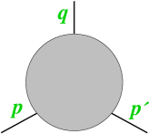
Figure 1: Three-point vertex function (9).

This correlator contains the triple-pole in the Minkowski region, namely,

$$\Gamma(p,p^{\prime},q)=\frac{ff^{\prime}}{(p^{2}-M^{2})({p^{\prime}}^{2}-{M^{\prime}}^{2})}F(q^{2})+\cdots,$$ (10)

where the form factor $F(q^{2})$ contains a pole at $q^{2}=M_{q}^{2}$:

$$F(q^{2})=\frac{f_{q}g_{MM^{\prime}M_{q}}}{(q^{2}-M_{q}^{2})}+\cdots.$$ (11)

Here, $g_{MM^{\prime}M_{q}}$ describes the $M\to M^{\prime}M_{q}$ strong transition; $f$, $f^{\prime}$, and $f_{M_{q}}$ are the decay constants of the mesons: $\langle 0|J(0)|M\rangle=f$, $\langle 0|j^{\prime}(0)|M^{\prime}\rangle=f^{\prime}$, and $\langle 0|j(0)|M_{q}\rangle=f_{q}$.

The three-point function satisfies the double spectral representation

$$\Gamma(p,p^{\prime},q)=\int\frac{ds}{s-p^{2}}\frac{ds^{\prime}}{s^{\prime}-{p^{\prime}}^{2}}\Delta(s,s^{\prime},q^{2})$$ (12)

A double Borel transformation $p^{2}\to\tau$, $p^{\prime 2}\to\tau^{\prime}$ and duality cuts in the $p^{2}$ and $p^{\prime 2}$ channels ioffe3pt ; radyushkin ; bakulev lead to

$$\exp(-M^{2}\tau)\exp(-M^{\prime 2}\tau^{\prime})F(q^{2})=\int\limits^{s_{\rm eff}}ds\exp(-s\tau)\int\limits^{s^{\prime}_{\rm eff}}ds^{\prime}\exp(-s^{\prime}\tau^{\prime})\Delta_{\rm OPE}(s,s^{\prime},q^{2})$$ (13)

Let us discuss this relation for two cases: for normal bilinear and for exotic four-quark currents.

2.1 Normal hadrons

An elastic or a transition form factor of a normal meson corresponds to the choice of the interpolating currents in Eq. (13) in the bilinear form, that is, $J,j,j^{\prime}=\bar{q}_{i}\hat{O}q_{j}$, with appropriate quark fields $q_{i,j}$ and a generic Dirac matrix $\hat{O}$. The perturbative part of the correlation function has the following structure:

$$\Gamma_{\rm OPE}(p^{2},p^{\prime 2},q^{2})=\Gamma_{0}(p^{2},p^{\prime 2},q^{2})+\alpha_{s}\Gamma_{1}(p^{2},p^{\prime 2},q^{2})+\cdots.$$ (14)

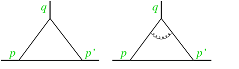
Figure 2: The OPE for the three-point function of the bilinear $\bar{q}q$ interpolating currents for normal mesons. The leading-order diagram and one of the radiative corrections are shown.

Already the one-loop leading-order diagram has a nonzero double-spectral density $\Delta_{0}(s,s^{\prime},q^{2})$ and therefore provides a nonzero contribution to the form factor (and, respectively, to $g_{MM^{\prime}M_{q}}$). Radiative corrections bagan ; fulvia ; braguta give essential contributions, increasingly important at larger $q^{2}$ anisovich ; blm2008plb . However, a reasonable estimate may be obtained already from the leading-order three-point function lm2012prd ; lm2012jpg ; blm2012prd ; ms2012prd .

2.2 Three-point function containing one exotic current

The interpolating current for the exotic state (for the sake of clarity, we focus to the case of tetraquarks, i.e., exotic states with four valence quarks) may be chosen in many different ways (see the discussion in the next section). Let us consider an interpolating current $\theta(x)$ of the following rather general form:

$$\theta(x)=\bar{q}_{1}(x)\hat{O}q_{2}(x)\bar{q}_{3}(x)\hat{O}q_{4}(x),$$ (15)

where $\hat{O}$ is an appropriate combination of Dirac and colour matrices and possibly also of (covariant) derivatives. The OPE for the correlation function $\Gamma^{\theta jj}=\langle T(\theta(x)j(y)j(z)\rangle$ containing one exotic current and two normal currents has the diagrammatic structure shown in Fig. 3 and reads

$$\Gamma^{\theta jj}_{\rm OPE}(p^{2},p^{\prime 2},q^{2})=\Pi(p^{\prime 2})\Pi(q^{2})+\alpha_{s}\Gamma_{\rm connected}(p^{2},p^{\prime 2},q^{2}).$$ (16)

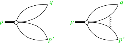
Figure 3: Perturbative expansion of the three-point function containing one exotic tetraquark current and two normal quark–antiquark currents.

As known from the general features of the Bethe-Salpeter equation, the disconnected diagrams are not related to the bound states. This is also clear from the following argument: Performing the Borel transformation $p^{2}\to\tau$ (one of the steps of a sum-rule analysis), the Borel image of the disconnected leading-order contribution vanishes. The connected diagrams, relevant for the exotic states, emerge at order $O(\alpha_{s})$ and higher. Thus, any attempt to extract, e.g., the tetraquark decay amplitude from the leading-order contribution is inconsistent. The common feature of all previous investigations of these decays by QCD sum rules (e.g., nielsen2010 ; nielsen2014 ; wang2014 ; nielsen2016 ) was the attempt to study tetraquark (and pentaquark) decays relying on the factorizable leading-order contribution, which intrinsically has no relation to tetraquark properties [which fact is evident from both the factorization property $\Gamma(p,p^{\prime},q)=\Pi(p^{\prime 2})\Pi(q^{2})$ and the large-$N_{c}$ behaviour of the QCD diagrams Weinberg ; knecht ; cohen ]. Therefore, the existing analyses should be strongly revised by calculating and taking into account the nonfactorizable two-loop $O(\alpha_{s})$ corrections. In other words, the “fall-apart” decay of exotic hadrons differs from the decay mechanism of ordinary hadrons and requires an appropriate treatment within QCD sum rules. The leading-order contribution is not related to the exotic-state decay, as is clear from its factorization property $\Gamma(p,p^{\prime},q)=\Pi(p^{\prime 2})\Pi(q^{2})$ and from the large-$N_{c}$ behaviour of the QCD diagrams. The calculation of the radiative corrections is mandatory for a reliable analysis of the properties of the exotic states.

3 Structure of the exotic states

Obviously, the exotic tetraquark states may have a rather complicated “internal” structure. The most popular scenarios for such a structure are a confined tetraquark state (i.e., a bound state in a confining potential between two colour-triplet diquarks) and a molecular “nuclear-physics-like” bound state in the system of two colourless mesons.

However, an important question about the structure of the exotic state — which to a large extent controls also its production mechanism — is not easy to answer jaffe : (i) by a combined colour–spinor Fierz rearrangement of the tetraquark interpolating current $D(x)$ one can express it in either diquark–antidiquark or meson–meson form; (ii) the same quantum numbers of the exotic interpolating current may be obtained by different combinations of its diquark–antidiquark or meson–meson bilinear parts.

3.1 Set of decay constants of exotic states

The simplest characteristic of a meson is its decay constant, i.e., the transition amplitude between the vacuum and the meson, induced by its interpolating current. For a heavy quarkonium state, the decay constant is analogous to its wave function at spatial origin, $\psi(r=0)$. Whereas an ordinary meson is described by one or few decay constants $\langle 0|\bar{q}_{1}O_{A}q_{2}|M\rangle=f_{A}$, exotic states have many decay constants, related to possible different structures of the interpolating four-quark currents; e.g., the interpolating currents may be chosen in “meson–meson” form $\langle 0|M_{12}(x)M_{34}(x)|\theta\rangle=f_{MM}$ with $M_{12}=\bar{q}_{1}Oq_{2}$, or in “diquark–diquark” form $\langle 0|\bar{D}^{a}_{13}(x)D^{a}_{24}(x)|\theta\rangle=f_{DD}$ with $D^{a}_{24}=\epsilon^{abd}(q^{b}_{c4})^{T}q^{d}_{2}.$ If, in some limit, a certain class of decay constants vanishes, one is eligible to say that the exotic state is, e.g., a pure molecular or a pure diquark–antidiquark state. In general, the mixing of different “components” seems unavoidable.

An appropriate tool to access the decay constants theoretically is the QCD sum rule for two-point functions, $\Pi^{(\theta\theta)}=\langle\theta(x)\theta(0)\rangle$ narison . Let us emphasize, however, that not all contributions to two-point functions of exotic interpolating currents are related to the properties of exotic states. The large-$N_{c}$ behaviour of the different diagrams should be the guiding principle for the selection of appropriate contributions, similar to selecting the connected contributions to three-point functions. After selecting the appropriate contributions to the two-point functions $\Pi_{\theta\theta}$, the set of sum rules should be studied and only then the answer about the structure of the observed narrow exotic candidates may be obtained.

3.2 Form factors of the exotic states

The appropriate quantities which describe the structure of bound states — both normal and exotic — are the form factors. For exotic states, these are the form factors related to the connected parts of the three-point functions involving two exotic interpolating currents, $\langle T(\theta\theta j)\rangle$; so far, no OPE calculations for the corresponding quantities are available in the literature.

4 Conclusions and Outlook

• The three-point (vertex) correlation functions for the normal bilinear quark currents show a crucial difference from the three-point correlation functions of exotic polyquark interpolating currents: the latter are described at leading order by disconnected diagrams, not related to strong decays of exotic hadrons. In the exotic-current case, the relevant diagrams start at order $O(\alpha_{s})$. This requires taking into account $O(\alpha_{s})$ corrections.

• Similar to the case of three-point functions, not all contributions to two-point correlation functions of exotic interpolating currents are related to the properties of the exotic bound state: the $N_{c}$ scaling may be the guiding principle for selecting the appropriate contributions.

• Our experience in the analysis of the normal hadrons proves that a truncated OPE for the correlation function does not enable one to study at the same time both the existence of the isolated ground state and its properties. However, if the mass of such a narrow bound state is known, the QCD-sum rule approach allows one to obtain reliable predictions for decay constants lms_fBetc and form factors hagop . The observed exotic-state candidates are narrow; therefore, any procedure for the extraction of their parameters from the OPE has the same features and the same challenges as for the normal hadrons.

D. M. was supported by the Austrian Science Fund (FWF) under project P29028-N27.

References

- (1) M. A. Shifman, A. I. Vainshtein, and V. I. Zakharov, Nucl. Phys. B 147, 385 (1979).
- (2) P. Colangelo and A. Khodjamirian, hep-ph/0010175.
- (3) B. L. Ioffe, Prog. Part. Nucl. Phys. 56, 232 (2006).
- (4) V. A. Novikov, M. A. Shifman, A. I. Vainshtein, and V. I. Zakharov, Nucl. Phys. B 249, 445 (1985).
- (5) C. T. H. Davies et al., PoS ConfinementX 042 (2012).
- (6) C. Dominguez, L. Hernandez, and K. Schilcher, JHEP 1507, 110 (2015).
- (7) B. Blok, M. Shifman, and D.-X. Zhang, Phys. Rev. D 57, 2691 (1998); 59, 019901(E) (1999); M. Shifman, hep-ph/0009131.
- (8) W. Lucha and D. Melikhov, Phys. Rev. D 73, 054009 (2006).
- (9) W. Lucha, D. Melikhov, and S. Simula, Phys. Lett. B 687, 48 (2010).
- (10) W. Lucha, D. Melikhov, and S. Simula, Phys. Rev. D 76, 036002 (2007); Phys. Lett. B 657, 148 (2007).
- (11) W. Lucha, D. Melikhov, and S. Simula, Phys. Lett. B 671, 445 (2009); Phys. Rev. D 79, 096011 (2009); J. Phys. G 37, 035003 (2010); D. Melikhov, Phys. Lett. B 671, 450 (2009).
- (12) B. L. Ioffe and A. V. Smilga, Phys. Lett. B 114, 353 (1982).
- (13) V. A. Nesterenko and A. V. Radyushkin, Phys. Lett. B 115, 410 (1982).
- (14) A. P. Bakulev and A. V. Radyushkin, Phys. Lett. B 271, 223 (1991).
- (15) E. Bagan, P. Ball, and P. Godzinsky, Phys. Lett. B 301, 249 (1993).
- (16) P. Colangelo, F. De Fazio, and N. Paver, Phys. Rev. D 58, 116005 (1998).
- (17) V. Braguta and A. Onishchenko, Phys. Lett. B 591, 255 (2004); 591, 267 (2004).
- (18) V. V. Anisovich, D. Melikhov, and V. Nikonov, Phys. Rev. D 52, 5295 (1995); 55, 2918 (1997).
- (19) V. Braguta, W. Lucha, and D. Melikhov, Phys. Lett. B 661, 354 (2008).
- (20) W. Lucha and D. Melikhov, Phys. Rev. D 86, 016001 (2012).
- (21) W. Lucha and D. Melikhov, J. Phys. G 39, 045003 (2012).
- (22) I. Balakireva, W. Lucha, and D. Melikhov, J. Phys. G 39, 055007 (2012); Phys. Rev. D 85, 036006 (2012).
- (23) D. Melikhov and B. Stech, Phys. Rev. D 85, 051901 (2012); Phys. Lett. B 718, 488 (2012).
- (24) M. Nielsen, F. S. Navarra, and S.-H. Lee, Phys. Rept. 497, 41 (2010).
- (25) F. S. Navarra and M. Nielsen, Mod. Phys. Lett. A 29, 1430005 (2014).
- (26) Z.-G. Wang and T. Huang, Nucl. Phys. A 930, 63 (2014).
- (27) J. M. Dias et al., Phys. Lett. B 758, 235 (2016).
- (28) S. Weinberg, Phys. Rev. Lett. 110, 261601 (2013).
- (29) M. Knecht and S. Peris, Phys. Rev. D 88, 036016 (2013).
- (30) T. D. Cohen and R. F. Lebed, Phys. Rev. D 89, 054018 (2014); 90, 016001 (2014).
- (31) R. L. Jaffe, Nucl. Phys. A 804, 25 (2008).
- (32) F. Fanomezana, S. Narison, and A. Rabemananjara, Nucl. Part. Phys. Proc. 258–259, 152 (2015); L. Albuquerque et al., Int. J. Mod. Phys. A 31, 1650093 (2016).
- (33) W. Lucha, D. Melikhov, and S. Simula, J. Phys. G 38, 105002 (2011); Phys. Lett. B 701, 82 (2011); Phys. Rev. D 88, 056011 (2013); Phys. Lett. B 735, 12 (2014); Phys. Rev. D 91, 116009 (2015).
- (34) W. Lucha, D. Melikhov, H. Sazdjian, and S. Simula, Phys. Rev. D 80, 114028 (2009).