Experimental preparation of topologically ordered states via adiabatic evolution

Abstract

Topological orders are a class of exotic states of matter characterized by patterns of long-range entanglement. Certain topologically ordered systems are proposed as potential realization of fault-tolerant quantum computation. Topological orders can arise in two-dimensional spin-lattice models. In this paper, we engineer a time-dependent Hamiltonian to prepare a topologically ordered state through adiabatic evolution. The other sectors in the degenerate ground-state space of the model are obtained by applying nontrivial operations corresponding to closed string operators. Each sector is highly entangled, as shown from the completely reconstructed density matrices. This paves the way towards exploring the properties of topological orders and the application of topological orders in topological quantum memory.

, ,

Keywords: topologically ordered state, adiabatic evolution, nuclear magnetic resonance

1 Introduction

The emergence of topological order in fractional quantum Hall effect has broadened our understanding of phases of matter [1, 2, 3]. Phases of matter are much richer than those describable by symmetry-breaking. In the framework of Landau theory [4, 5, 6], all phases of matter were thought to be characterized by different symmetries and their phase transitions were associated with broken symmetries. The discovery of distinct fractional quantum Hall states, which have exactly the same symmetries [3, 7] were the first solid evidence that the Landau symmetry-breaking paradigm is inadequate. In particular, these phases cannot be distinguished by local order parameters. Microscopically, topological order corresponds to patterns of long-range entanglement [8]. Topological entanglement entropy for example can be used as a nonlocal order parameter to (partially) identify the topological phases [9, 11].

Topological orders are of basic scientific interest not only for their topological properties in condensed matter physics [12, 13, 14, 9, 10] but also for their potential application in fault-tolerant quantum computation [15, 16, 17, 18]. This mainly relies on the robustness of degenerate ground states [12] and their patterns of long-range entanglement [8]. Topologically ordered states support degenerate ground states when the system is placed in a geometry with non-trivial topology. In two dimensions, its ground-state degeneracy depends on the genus of the Riemann surface it lives in. Because any two orthogonal sectors in ground-state sub-space are related by non-contractible loop operators, local perturbations only lead to local errors that can be easily detected and corrected. This translates into effective correction of both phase flip and bit flip errors in explicit models. These properties are attractive for constructing a robust memory register [19, 20].

Two-dimensional spin-lattice models exhibit topological orders [15, 21, 22]. However, such models usually include many-body interactions that have not been found in natural physical systems. Feynman suggested that [23] a well-controlled quantum system can be used for the efficient simulation of other quantum systems. This implies that one can bypass limitations set by natural materials, and study detailed quantum phenomenon of exotic systems via quantum simulations. Quantum simulation could be realized by various physical platforms such as trapped ion [24], superconducting circuit [25], nuclear magnetic resonance (NMR) [26], and so on. There have been a lot of successful demonstrations in simulating condensed matter physics [27, 28, 29], high-energy physics [30], atomic physics [31], quantum chemistry [32, 33], and cosmology [34, 35]. Quantum simulation thus provides a powerful tool to investigate topological order [36, 37, 38, 39, 40].

In this paper, we realize the Hamiltonian of Wen-plaquette spin-lattice model with $Z_{2}$ topological orders in an NMR system. There are four-fold degenerate ground states when the Hamiltonian is chosen to have doubly periodic boundary condition, i.e., we have placed the system on a torus. Following the method proposed by Hamma et al. [41], a topologically ordered state is experimentally prepared through adiabatically engineering the time-dependent Hamiltonian. The other sectors in the degenerate ground-state subspace are obtained by performing two nontrivial closed string operations. We reconstruct the density matrices for each sector using complete quantum state tomography technology. The results show that each sector exhibits maximum entanglement. It is a central step to prepare degenerate topologically ordered states for studying topological quantum phase transition [36], measuring modular matrices [38], constructing robust quantum memory, and so on.

2 Wen-plaquette model

The Wen-plaquette model building on an $N\times N$ square lattice is illustrated in figure 1, where each site accommodates a spin $1/2$ [22]. Its Hamiltonian is written as

$$H_{\textrm{Wen}}=-\sum_{\textrm{white plaquettes}}X_{p}-\sum_{\textrm{yellow plaquettes}}Z_{p}.$$ (1)

Here $X_{p}=\prod_{j\in\partial p}\sigma_{j}^{x},Z_{p}=\prod_{j\in\partial p}\sigma_{j}^{z}$ are the plaquette operators that act on four spins surrounding a plaquette $p$, and $\sigma_{j}^{\alpha}$’s stand for Pauli operators. This is an exactly solvable model because $[X_{p},Z_{p^{\prime}}]=0$ for all $p$ and $p^{\prime}$. One can show that both the Wen-plaquette model and the toric code model describe the $Z_{2}$ topological order. The ground state manifold $\mathcal{L}$ is given by

$$\{|\psi_{g}\rangle\in\mathcal{H}:X_{p}|\psi_{g}\rangle=Z_{p}|\psi_{g}\rangle=|\psi_{g}\rangle\textrm{ for all }p\}.$$ (2)

The ground state degeneracy $D$ depends on the genus g of the Riemann surface, i.e., $D=2^{2\textsf{g}}$. If the Riemann surface has genus g, we can define $2\textsf{g}$ non-contractible strings that connect different topological sectors in $\mathcal{L}$. For example, on a torus its four-fold degenerate ground states can be described by using two nontrivial closed strings of $\gamma_{1}$ and $\gamma_{2}$,

$$|\psi_{g}^{(\nu_{1},\nu_{2})}\rangle=\mathcal{T}_{x}^{\nu_{1}}(\gamma_{1})\mathcal{T}_{x}^{\nu_{2}}(\gamma_{2})|\psi_{g}^{(0,0)}\rangle,\nu_{1},\nu_{2}=0,1.$$ (3)

Here the string operators are defined as $\mathcal{T}_{x}(\gamma)=\prod_{j\in\gamma}\sigma_{j}^{x}$. The initial topological sector $|\psi_{g}^{(0,0)}\rangle$ of $\mathcal{L}$ is given by the equal superposition of all contractible closed strings including no string (or say the string is a point). It is not difficult to find that $\mathcal{T}_{x}(\gamma_{3})=\prod_{p\in f}X_{p}$, namely, the product of all plaquette operators in the surface $f$ that satisfies $\partial f=\gamma_{3}$. And for the case of no string, its corresponding operator is the identity matrix $I$. All operators corresponding to such strings form a group denoted as $\mathcal{G}$. Its elements are generated by $n=(N^{2}-2)/2$ independent plaquette operators in the white sublattice, i.e., $g_{s}=\prod_{p=1}^{n}X_{p}^{s_{p}},s_{p}\in\{0,1\}$. Thus,

$$|\psi_{g}^{(0,0)}\rangle=\frac{1}{\sqrt{|\mathcal{G}|}}\sum_{g_{s}\in\mathcal{G}}^{|\mathcal{G}|}g_{s}|00\cdots\rangle,$$ (4)

where $|\mathcal{G}|$ is the number of elements in $\mathcal{G}$. Also, $|0\rangle$ stands for spin-up states along the $z$ axis. According to the closure of group and the commutation relations, we can prove that $X_{p}|\psi_{g}^{(\nu_{1},\nu_{2})}\rangle=Z_{p}|\psi_{g}^{(\nu_{1},\nu_{2})}\rangle=|\psi_{g}^{(\nu_{1},\nu_{2})}\rangle$ for all $p,\nu_{1},\nu_{2}$. Therefore, the states of $|\psi_{g}^{(\nu_{1},\nu_{2})}\rangle$ constructed from equations (3) and (4) are indeed the ground states of the Hamiltonian (1). Besides, it shows that $\langle\psi_{g}^{(\nu_{1},\nu_{2})}|\psi_{g}^{(\nu_{1}^{{}^{\prime}},\nu_{2}^{{}^{\prime}})}\rangle=\delta_{\nu_{1},\nu_{1}^{{}^{\prime}}}\delta_{\nu_{2},\nu_{2}^{{}^{\prime}}}$, meaning that, different topological sectors are orthogonal.

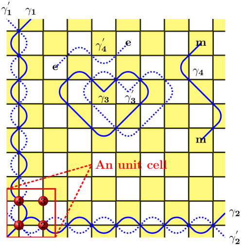
Figure 1: The Wen-plaquette spin-lattice model on a torus. When $N$ is even, there exist two sublattice denoted by white and yellow. The blue solid strings ($\gamma_{1}\sim\gamma_{4}$) and their dual dashed strings ($\gamma_{1}^{{}^{\prime}}\sim\gamma_{4}^{{}^{\prime}}$) are defined in the yellow sublattice and in the white sublattice, respectively. $e$ and $m$ represent the elementary excitations (anyons): electric charge and magnetic vortex, which in pairs generated by open string operators. The red box is an unit cell of square lattice. The red balls represent spins placing on each site.

A unit cell on a torus is illustrated in the red box of figure 1, which consists of $2\times 2$ spins. Although it is the smallest system, the properties of topological orders are still presented in the Wen-plaquette spin-lattice model since they describe fixed wavefunction [22]. This validity also follows from the fairly short-range spin-spin correlations [36]. Under the periodic boundary condition, we can get the Hamiltonian

$$\hat{H}_{\textrm{Wen}}^{4}=-2(X_{p}+Z_{p}).$$ (5)

Two nontrivial loop operators are $\mathcal{T}_{x}(\gamma_{1})=\sigma_{1}^{x}\sigma_{4}^{x}$ and $\mathcal{T}_{x}(\gamma_{2})=\sigma_{1}^{x}\sigma_{2}^{x}$ and all contractible closed-string operators form a group, i.e., $\mathcal{G}=\{I,X_{p}\}$, which are generated by one independent plaquette operator, i.e., $X_{p}$. So from equations (3) and (4), the four-fold degenerate ground states can be described as follows,

$$|\psi_{g}^{(0,0)}\rangle=(|0000\rangle+|1111\rangle)/\sqrt{2}~{}$$ (6)

$$|\psi_{g}^{(0,1)}\rangle=(|0011\rangle+|1100\rangle)/\sqrt{2}~{}$$

$$|\psi_{g}^{(1,0)}\rangle=(|0110\rangle+|1001\rangle)/\sqrt{2}~{}$$

$$|\psi_{g}^{(1,1)}\rangle=(|0101\rangle+|1010\rangle)/\sqrt{2}.$$

Here we work with basis states which are eigenstates of $\sigma_{z}$ at each site. The theory shows that each topological sector in equation (6) is a maximally entangled state through stochastic local quantum operation assisted by classical communication (SLOCC) [42, 43].

3 Experiment

The experiment was carried out on a Bruker AV-400 spectrometer ($9.4T$) at room temperature $T=300$ K. We chose one ¹³C and three ¹⁹F nuclear spins of Iodotrifluroethylene (C₂F₃I) as a 4-qubit quantum simulator. Its molecular structure and relevant parameters are shown in figures 2(a) and 2(b). The natural Hamiltonian of this system under weak coupling approximation is

$$\hat{H}_{\textrm{NMR}}=\sum_{j=1}^{4}\frac{\omega_{j}}{2}\hat{\sigma}_{z}^{j}+\sum_{j<k,=1}^{4}\frac{\pi J_{jk}}{2}\hat{\sigma}_{z}^{j}\hat{\sigma}_{z}^{k},$$ (7)

where $\omega_{j}$ represents the chemical shift of spin $j$ and $J_{jk}$ the coupling constant between spin $j$ and spin $k$.

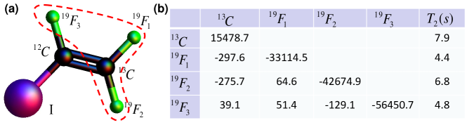
Figure 2: (a) Molecular structure of lodotrifluroehtylene, where ¹³C and three ¹⁹F nuclei are used as a 4-qubit quantum simulator. (b) The chemical shifts and the coupling constants (in units of Hz) are on and below the diagonal in the table.The spin-lattice relaxation times ($T_{1}$) are $21$ s for ¹³C and $12.5$ s for ¹⁹F.

The quantum system was firstly prepared in the initial pseudo-pure state (PPS):$\hat{\rho}_{0000}=\frac{1-\epsilon}{16}\mathbb{I}+\epsilon|0000\rangle\langle 0000|$ using line-selective approach [44], with $\mathbb{I}$ representing $16\times 16$ identity operator and $\epsilon\approx 10^{-5}$ the polarization. Note that $|0000\rangle$ is the ground state of $\hat{H}_{0}=-\sum_{j=1}^{4}\hat{\sigma}_{j}^{z}$. We then adiabatically prepare the ground state $|\psi_{g}^{(0,0)}\rangle$ of Wen-plaquette model by varying the time-dependent Hamiltonian sufficiently slowly,

$$\hat{H}(t)=[1-s(t)]\hat{H}_{0}+s(t)\hat{H}_{\textrm{Wen}}^{4},$$ (8)

where the parameter function $s(t)$ increases monotonically from 0 at $t=0$ to 1 at $t=T$. The energy levels of $\hat{H}(t)$ as the function of the parameter $s(t)$ are shown in figure 3(a). The red and green curves represent the ground-state and first excited-state energies, respectively. To ensure that the system is prepared to the ground state of target Hamiltonian at $t=T$, the variation of the control parameter has to be slow sufficiently, i.e., satisfing the adiabatic condition [45],

$$\frac{\langle\psi_{g}|\frac{\partial\hat{H}(t)}{\partial s(t)}\frac{\partial s(t)}{\partial t}|\psi_{e}\rangle}{(\varepsilon_{e}-\varepsilon_{g})^{2}}=\epsilon\ll 1.$$ (9)

This condition determines the optimal sweep of control parameter $s(t)$, which was interpolated with M discretized scan steps. The duration of each step is defined as $\tau=T/M$. Thus the adiabatic condition is satisfied when both $T,M\to\infty$ and $\tau\to 0$. To determine the optimal $M$ in the adiabatic transfer, we numerically simulated the minimum fidelity $F_{\textrm{min}}$ encountered during the scan as a function of the number of steps, as shown in figure 3(b), where we fixed the total evolution time $T=2.9982$. The fidelity is calculated as the overlap of the theoretical and simulated ground states at each step of adiabatic evolution. In the experiment, we discretized into $M=7$ steps and the minimal fidelity $F_{\textrm{min}}$ is $\geq 0.99$, which indicates that the state of the system is always close to its instantaneous ground state in the whole adiabatic passage.

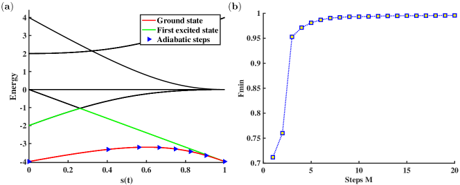
Figure 3: (a) The energy-level diagram of the time-dependent Hamiltonian $\hat{H}[s(t)]$. The red and green curves represent the energies of ground state and first excited state, respectively. The blue $\vartriangleright$ points represent the $M=7$ interpolations on the line of $s(t)$ with the same time interval $\tau$. (b) The minimum fidelity $F_{\textrm{min}}$ during the adiabatic passage as the function of the number of steps $M$.

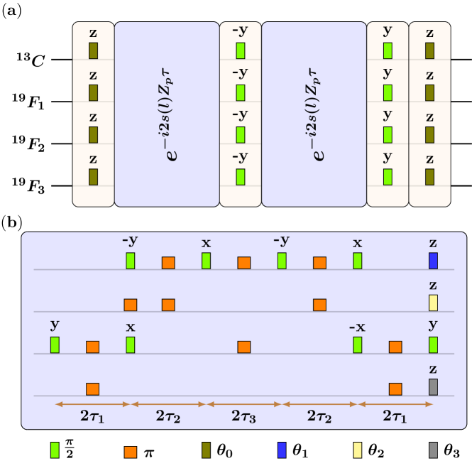
Figure 4: Pulse sequences for (a) implementing the adiabatic evolution of $l_{th}$ step, and (b) effectively creating four-body interaction, i.e., $Z_{p}=\hat{\sigma}_{z}^{1}\hat{\sigma}_{z}^{2}\hat{\sigma}_{z}^{3}\hat{\sigma}_{z}^{4}$, where $\tau_{1}=1/4J_{34},\tau_{2}=1/4J_{12},\tau_{3}=2s(l)\tau/\pi J_{13},\theta_{0}=[1-s(l)]\tau/2,\theta_{1}=-\omega_{1}/J_{34},\theta_{2}=-4\omega_{2}s(l)\tau/\pi J_{13}$ and $\theta_{3}=\omega_{4}/J_{12}+4\omega_{4}s(l)\tau/\pi J_{13}$.

The adiabatic evolution for each step can be decomposed by Suzuki-Trotter expansion as

$$e^{-i\hat{H}[s(l)]\tau}=e^{-i[1-s(l)]\hat{H}_{0}\tau/2}e^{-is(l)\hat{H}_{\textrm{Wen}}^{4}\tau}e^{-i[1-s(l)]\hat{H}_{0}\tau/2}+O(\tau^{3}),$$ (10)

with $l=0,1,\cdots,M$. This expansion faithfully represents the targeted evolution if the duration $\tau$ provided is kept sufficiently short. Due to $[X_{p},Z_{p}]=0$, we have

$$e^{-is(l)\hat{H}_{\textrm{Wen}}^{4}\tau}=\prod_{j=1}^{4}\hat{R}_{j}^{y}(\frac{\pi}{2})e^{i2s(l)Z_{P}\tau}\prod_{j=1}^{4}\hat{R}_{j}^{y}(-\frac{\pi}{2})e^{i2s(l)Z_{p}\tau}.$$ (11)

Here the four-body interaction $Z_{p}$ is effectively created by a combination of RF pulses and free evolutions of NMR system [46, 47]:

$$e^{-i2s(l)Z_{p}\tau}=\hat{R}_{1}^{z}(\theta_{1})\hat{R}_{2}^{z}(\theta_{2})\hat{R}_{4}^{z}(\theta_{3})\hat{R}_{3}^{y}(\frac{\pi}{2})e^{-i\hat{H}_{\textrm{NMR}}\tau_{1}}\hat{R}_{3}^{y}(\pi)\hat{R}_{4}^{y}(\pi)e^{-i\hat{H}_{\textrm{NMR}}\tau_{1}}\hat{R}_{1}^{y}(-\frac{\pi}{2})$$ (12)

$$\cdot\hat{R}_{3}^{x}(-\frac{\pi}{2})e^{-i\hat{H}_{\textrm{NMR}}\tau_{2}}\hat{R}_{1}^{y}(\pi)\hat{R}_{2}^{y}(\pi)e^{-i\hat{H}_{\textrm{NMR}}\tau_{2}}\hat{R}_{1}^{x}(\frac{\pi}{2})e^{-i\hat{H}_{\textrm{NMR}}\tau_{3}}\hat{R}_{1}^{x}(\pi)\hat{R}_{3}^{x}(\pi)$$

$$\cdot e^{-i\hat{H}_{\textrm{NMR}}\tau_{3}}\hat{R}_{1}^{x}(\frac{\pi}{2})e^{-i\hat{H}_{\textrm{NMR}}\tau_{2}}\hat{R}_{1}^{y}(\pi)\hat{R}_{2}^{y}(\pi)e^{-i\hat{H}_{\textrm{NMR}}\tau_{2}}\hat{R}_{1}^{y}(-\frac{\pi}{2})\hat{R}_{3}^{x}(\pi/2)$$

$$\cdot\hat{R}_{2}^{y}(\pi)e^{-i\hat{H}_{\textrm{NMR}}\tau_{1}}\hat{R}_{3}^{x}(\pi)\hat{R}_{4}^{x}(\pi)e^{-i\hat{H}_{\textrm{NMR}}\tau_{1}}\hat{R}_{3}^{y}(\frac{\pi}{2}),$$

where $\hat{R}_{j}^{\alpha}(\theta)=e^{-i\theta\hat{\sigma}_{j}^{\alpha}/2}(\alpha=x,y,z)$. Therefore, the adiabatic evolution for each step can be implemented by the pulse sequences, as shown in figures 4(a) and 4(b). This simulation method is in principle efficient, provided the decoherence time is long enough. In order to overcome the accumulated pulse errors and the decoherence, each step of adiabatic evolution $e^{-i\hat{H}[s(l)]\tau}$ ($l=0,1,2,...,M$) was optimized by the gradient ascent pulse engineering (GRAPE) algorithm [48]. The GRAPE pulses of $e^{-i\hat{H}[s(l)]\tau}$ were designed to have the pulse length of 30 $ms$ and theoretical fidelity of over 0.99 in experiments.

Once the initial topologically ordered state $|\psi_{g}^{(0,0)}\rangle$ was prepared via the adiabatic evolution, the other topological sectors in $\mathcal{L}$ were obtained by performing non-contractible string operators $\mathcal{T}_{x}^{\nu_{1}}(\gamma_{1})\mathcal{T}_{x}^{\nu_{2}}(\gamma_{2})$ on $|\psi_{g}^{(0,0)}\rangle$. Due to $\langle\psi_{g}^{(\nu_{1},\nu_{2})}|\dot{H}|\psi_{g}^{(\nu_{1}^{{}^{\prime}},\nu_{2}^{{}^{\prime}})}\rangle=0$ ($\nu_{1}\neq\nu_{1}^{{}^{\prime}}$ or $\nu_{2}\neq\nu_{2}^{{}^{\prime}}$), the transition between different topological sectors are forbidden during the adiabatic evolution. These nontrivial operators make it possible to have experimental access to different topological sectors. The resulting ${}^{13}C$ spectra for different quantum states are illustrated in figure 5, after a readout pulse $\hat{R}_{1}^{y}(\frac{\pi}{2})$ acting on ${}^{13}C$ observable nucleus. Figures 5(a) $\sim$ 5(d) correspond to the spectra of $|\psi_{g}^{(0,0)}\rangle,|\psi_{g}^{(0,1)}\rangle,|\psi_{g}^{(1,0)}\rangle$, and $|\psi_{g}^{(1,1)}\rangle$, respectively. To further confirm the experiments, we reconstructed the quantum state density matrices using the complete tomography technology [49]. The coefficients of 256 operators for a full density matrix of four-qubit state can be obtained by performing 44 independent experiments. These readout pulses are shown in Table. 1, which involve 28 local rotations and 3 SWAP gates. They were realized by GRAPE pulses with the length of 400 $\mu s$ for local rotations, 9 $ms$ for SWAP gates between ${}^{13}C$ and $F_{1}$, $F_{2}$, and 30 $ms$ for SWAP gate between ${}^{13}C$ and $F_{3}$, respectively. The reconstructed results are shown in figure 6, with the fidelities being $96.46\%,96.59\%,96.06\%\textrm{ and }96.06\%$ for four topological sectors in $\mathcal{L}$, respectively. The receivable fidelities ensure that it is successful to adiabatically prepare the topological orders with patterns of long-range entanglement.

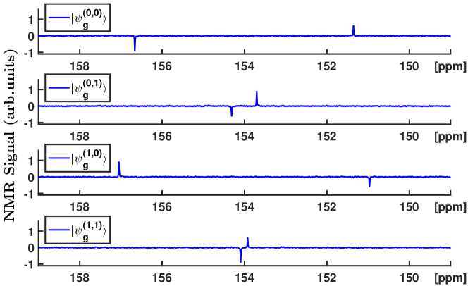
Figure 5: Experimental ${}^{13}C$ spectra corresponding to four topological sectors i.e., $|\psi_{g}^{(0,0)}\rangle,|\psi_{g}^{(0,1)}\rangle,|\psi_{g}^{(1,0)}\rangle$, and $|\psi_{g}^{(1,1)}\rangle$ from top to bottom, respectively.

Table 1: Readout pulses for fully reconstructing a density matrix of 4-qubit state. Here E is the unit operator; X and Y denote a $\pi/2$ rotation along $x$ and $y$ axis; SWAP_ij represents a SWAP gate between spin $i$ and $j$ in order to transfer the ¹⁹F information to ¹³C, and then all signals are obtained from the ¹³C spectra.

EEEE, EXEE, EYEE, EEXE, EXXE, EYXE, EEYE, EXYE, EYYE, EEEX, EXEX,
EYEX, EEXX, EXXX, EYXX, EEYX, EXYX, EYYX, EEEY, EXEY, EYEY, EEXY,
EXXY, EYXY, EEYY, EXYY, EYYY, YEEE, EEEE*$\textrm{SWAP}_{12}$, EEXE*$\textrm{SWAP}_{12}$,
EEYE*$\textrm{SWAP}_{12}$, EEEX*$\textrm{SWAP}_{12}$, EEXX*$\textrm{SWAP}_{12}$, EEYX*$\textrm{SWAP}_{12}$, EEEY*$\textrm{SWAP}_{12}$,
EEXY*$\textrm{SWAP}_{12}$, EEYY*$\textrm{SWAP}_{12}$, EEE*$\textrm{SWAP}_{12}$, EEEE*$\textrm{SWAP}_{13}$, EEEX*$\textrm{SWAP}_{13}$,
EEEY*$\textrm{SWAP}_{13}$, YEEE*$\textrm{SWAP}_{13}$, EEEE*$\textrm{SWAP}_{14}$, YEEE*$\textrm{SWAP}_{14}$.

These experimental results are in good agreement with theoretical expectations. The relatively minor deviations can be attributed mostly to the imperfections of adiabatic approximation, GRAPE pulses and the spectral integrals. The theoretical infidelities of adiabatic approximation and GRAPE pulses are around $1\%$. Taking both errors into account, the numerical simulation gives the fidelities of $97.59\%,97.96\%,97.56\%\textrm{ and }97.75\%$ for four topological sectors. Though we used the spectral fitting method in experiments, there are about $1\%\sim 1.5\%$ errors from the spectral integrals by the comparison of the simulated and experimental results.

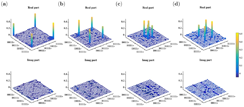
Figure 6: Experimental reconstructed density matrices for different topological sectors, that is, $|\psi_{g}^{(0,0)}\rangle,|\psi_{g}^{(0,1)}\rangle,|\psi_{g}^{(1,0)}\rangle$, and $|\psi_{g}^{(1,1)}\rangle$ corresponding to (a)$\sim$(d), respectively. The top an bottom represent the real parts and imaginary parts.

4 Discussion and conclusion

The Wen-plaquette spin-lattice model with $Z_{2}$ topological order is supported by four-body interactions, which is very rare and yet to be found in naturally occurring systems. Quantum simulation provides a powerful means to investigate these systems. Using an NMR simulator, we realized the model on a $2\times 2$ lattice on a torus. A topologically ordered state was experimentally prepared through adiabatically engineering the time-dependent Hamiltonian and the other sectors in the degenerate ground-state manifold were obtained by performing two non-contractible string operations. The experimental results were confirmed by the complete quantum state tomography. From the reconstructed density matrices, it shows that each topological sector is maximally entangled. The experiment demonstrated the feasibility of adiabatic method to prepare topological orders. In Ref. [41], it was also shown that the adiabatic timescale T scales at worst only as $\sqrt{n}$ for a system of $n$ spins, which means that we can apply the method to larger and more generic systems. The successful preparation of different topological sectors in degenerate ground-state manifold is crucial towards further study of robust properties of topological phase, and initial construction of topologically fault tolerant quantum memory.

References

References

- [1] Wen X G 1990 Int. J. Mod. Phys. B 4 239
- [2] Wen X G 2004 Quantum Field Theory of Many-Body Systems (Oxford University Press, Oxford)
- [3] Tsui D C, Stormer H L and Gossard A C 1982 Phys. Rev. Lett. 48 1559
- [4] Sachdev S 1999 Quantum Phase Transition (Cambridge University. Press, Cambrige)
- [5] Landau L D 1937 Phys. Z. Sowjetunion 11 26
- [6] Ginzburg V L and Landau L D 1950 J. Exp. Eheor. Phys. 20 1064
- [7] Laughlin R B 1983 Phys. Rev. Lett. 50 1395
- [8] Chen X, Gu Z C and Wen X G 2010 Phys. Rev. B 82 155138
- [9] Kitaev A and Preskill J 2006 Phys. Rev. Lett. 96 110404
- [10] Levin M and Wen X G 2006 Phys. Rev. Lett. 96 110405
- [11] Hamma A, Zhang W, Haas S and Lidar D A 2008 Phys. Rev. B 77 155111
- [12] Wen X G and Niu Q 1990 Phys. Rev. B. 41 9377
- [13] Arovas D, Schrieffer J R and Wilczek F 1984 Phys. Rev. Lett. 53 722
- [14] X. G. Wen, Adv. Phys. 44, 405 (1995).
- [15] Kitaev A 2003 Ann. Phys. (N.Y.) 303 2
- [16] Nayak C et al2008 Rev. Mod. Phys. 801083
- [17] Stern A and Lindner N H 2013 Science 339 1179-1181
- [18] Freedman M H, Kitaev A, Larsen M J and Wang Z 2003 Bull. Am. Math. Soc. 40 31
- [19] Dennis E et al2002 J. Math. Phys. 43 4452
- [20] Jiang L et al2008 Nat. Phys. 4 482-488
- [21] Kitaev A 2006 Ann. Phys. (N.Y.) 321 2
- [22] Wen X G 2003 Phys. Rev. Lett. 90 016803
- [23] Feynman R P 1982 Int. J. Theor. Phys. 21 467
- [24] Friedenauer A, Schmitz H, Glueckert J T, Porras D and Schaetz T 2008 Nat. Phys. 4 757
- [25] Clarke J and Wilhelm F K 2008 Nature (London) 453 1031
- [26] Vandersypen L M K and Chuang I L 2005 Rev. Mod. Phys. 76 1037
- [27] Peng X H, Du J F and Suter D 2005 Phys. Rev. A 71 012307
- [28] Kim K et al2010 Nature 465 590
- [29] Kandala A et al2017 Nature 549 242
- [30] Li K, Han M, Long G, Wan Y, Lu D, Zeng B and Laflamme R 2017 arXiv: 1702. 00365
- [31] Bernien H et al2017 Nature 551 579
- [32] Du J F et al2010 Phys. Rev. Lett. 104 030502
- [33] Lanyon B P et al2010 Nat. Chem. 2 106
- [34] Nation P D, Blencowe M P, Rimberg A J and Buks E 2009 Phys. Rev. Lett. 103 087004
- [35] Georgescu I M, Ashhab S and Nori F 2014 Rev. Mod. Phys. 86 153
- [36] Peng X H, Luo Z H, Zheng W Q, Kou S P, Suter D and Du J F 2014 Phys. Rev. Lett. 113 080404
- [37] Luo Z et al2016 Phys. Rev. A. 93 052116
- [38] Luo Z H, Li J, Li Z K, Hung L Y, Wan Y D, Peng X H and Du J F 2018 Nat. Phys 14 160-165
- [39] Kong F et al2016 Phys. Rev. Lett. 117 060503
- [40] Li K, Wan Y, Hung L, Lan T, Long G, Lu D, Zeng B and Laflamme R 2017 Phys. Rev. Lett. 118 080502
- [41] Hamma A and Lidar D A 2008 Phys. Rev. Lett. 100 030502
- [42] Verstraete F, Dehaene J, De Moor B and Verschelde H 2002 Phys. Rev. A. 65 052112
- [43] Regula B, Martino S D, Lee S and Adesso G 2014 Phys. Rev. Lett. 113 110503
- [44] Peng X, Zhu X, Fang X, Feng M, Gao K, Yang X and Liu M 2001 Chem. Phys. Lett. 340 509
- [45] Messiah A 1976 Quantum Mechanics (Wiley, New York)
- [46] Tseng C H et al1999 Phys. Rev. A 61 012302
- [47] Peng X H, Zhang J F, Du J F and Sutter D 2009 Phys. Rev. Lett 103 140501
- [48] Khaneja N, Reiss T, Kehlet C, Schulte Herbrüggen T and Glaser S J 2005 J. Magn. Reson 172 296
- [49] Lee J S 2002 Phys. Lett. A 305 349–353