Global anomalous transport of ICRH- and NBI-heated fast ions

Abstract

By taking advantage of the trace approximation, one can gain an enormous computational advantage when solving for the global turbulent transport of impurities. In particular, this makes feasible the study of non-Maxwellian transport coupled in radius and energy, allowing collisions and transport to be accounted for on similar time scales, as occurs for fast ions. In this work, we study the fully-nonlinear ITG-driven trace turbulent transport of locally heated and injected fast ions. Previous results indicated the existence of MeV-range minorities heated by cyclotron resonance, and an associated density pinch effect. Here, we build upon this result using the t3core code to solve for the distribution of these minorities, consistently including the effects of collisions, gyrokinetic turbulence, and heating. Using the same tool to study the transport of injected fast ions, we contrast the qualitative features of their transport with that of the heated minorities. Our results indicate that heated minorities are more strongly affected by microturbulence than injected fast ions. The physical interpretation of this difference provides a possible explanation for the observed synergy when NBI heating is combined with ICRH. Furthermore, we move beyond the trace approximation to develop a model which allows one to easily account for the reduction of anomalous transport due to the presence of fast ions in electrostatic turbulence.

• Submitted 25 Aug 2016

Fast ions are an important component of a fusion device, being responsible for a portion of heating required to bring tokamaks and stellarators up to fusion-relevant temperatures. Various phenomena can cause radial transport and hence a redistribution of this energy, including: neoclassical transport, transport from nonaxisymmetric magnetic “ripples”, stochastic magnetic field regions, Alfvén waves driven unstable by the fast ions themselves, and microturbulence. This latter effect is what we focus on in this work, taking advantage of recently developed tools to study the coupled radius-energy phase space transport of trace non-Maxwellian species.

With the ion cyclotron resonance heating (ICRH) technique, electromagnetic waves are launched into the plasma at a frequency resonant with that of ion cyclotron motion at some locations. Under certain circumstances, a very small population of minority ions can very efficiently absorb the power and be heated up to MeV-range energies [1]. Previous results indicated that the effect of microturbulence on these heated minorities is to cause a density “pinch” of fast ions against their temperature gradient [2], an effect which is also expected from the quasilinear diffusion coefficients of Maxwellian fast ions [3]. Another auxiliary heating scheme is neutral beam injection (NBI) in which an energetic beam of neutral particles is injected into the plasma, where they collide with thermal ions, ionizing and giving up their energy. This effectively results in a high energy “source” of fast ions taken from the bulk thermal population, mimicking the birth of alpha particles in fusion reactions.

We consider two classes of fast ions in this work: “heated”, where heat is supplied to an already-present species; and “injected”, which involves fast ions entering the plasma at high energy and slowing-down via collisions. The ICRH-heated minorities are an example of the former category, while NBI ions and alpha particles are examples of the latter. Although NBI heating profiles are unlikely to be similar to ICRH ions in real experiments, to assist in directly comparing both types, we will be using the same boundary conditions and energy deposition profile.

This article is organized as follows. In Sec. 1, we introduce our framework for solving the transport problem and describe the case we simulate. In Sec. 2, we describe and interpret our results from the t3core transport simulations, contrasting the behavior of heated and injected fast ions. Finally, in Sec. 3, we improve upon the trace approximation by developing a simple model to adjust the bulk plasma anomalous transport when fast ions are present in significant quantities.

1 Description of the problem

The method we use to solve the multiscale transport problem is based on the trace approximation, in which the fast ions do not have an effect on the turbulence. In a later section, we provide corrections to this approximation. For now, assuming the trace approximation holds, the pitch-angle averaged low-collisionality transport equation reads [4, 5]:

$$\frac{\partial F_{0}}{\partial t}+\frac{1}{V^{\prime}}\frac{\partial}{\partial r}V^{\prime}\Gamma_{r}+\frac{1}{v^{2}}\frac{\partial}{\partial v}v^{2}\Gamma_{v}=S,$$ (1)

where $S$ is the source; $V(r)$ is the volume enclosed by the flux surface labelled by its half-width $r$; $\Gamma_{r}$ is the turbulent radial flux of fast ions as a function of speed $v$; and $\Gamma_{v}$ includes all forms of transport in energy: turbulent energy exchange, direct heating, collisional diffusion and slowing-down. Upon pitch-angle averaging to obtain Eq. (1), we eliminate the pitch-angle scattering from both collisions and turbulence. However, in order to obtain a closed equation for the pitch-angle averaged distribution function $F_{0}$, we neglect the pitch angle dependence of the turbulent diffusivities (which multiply derivatives of $F_{0}$). According to the scalings of Ref. [6], this assumption is incorrect. However, the numerical results of Ref. [7] seem to indicate a very weak dependence of the diffusivity on pitch angle, at least at high energy and for non-extreme pitch angles (e.g. $\xi\lesssim 0.99$). With the caveat that a more complete treatment includes the pitch-angle dependence of the turbulent transport, we proceed to apply the trace approximation [8] to write the fluxes in terms of energy-dependent diffusivities as:

$$\Gamma_{r}=-D_{rr}\frac{\partial F_{0}}{\partial r}-D_{rv}\frac{\partial F_{0}}{\partial v}$$ (2)

$$\Gamma_{v}=-D_{vr}\frac{\partial F_{0}}{\partial r}-v\nu_{s}F_{0}-\left(\frac{1}{2}v^{2}\nu_{\|}+D_{vv}+\frac{P}{3n_{f}m}\right)\frac{\partial F_{0}}{\partial v},$$ (3)

where $\nu_{s}$ and $\nu_{\|}$ are the slowing-down and parallel velocity diffusion collision frequencies [9] summed over all bulk species, $P(r)$ is the heating power per unit volume, $m$ is the fast ion mass, and $n_{f}$ is the local fast ion density. Whether the source $S$ or injected power $P$ is used to inject energy into the system is the difference between “injected” and “heated” fast ions discussed above, and this is a distinction we will continue to make throughout this work. The form of the heating term in Eq. (3) is the same as the equation used by Ref. [10] for the isotropic part of the ICRH-heated distribution. Equations (1), (2), and (3) form a closed two-dimensional partial differential equation and is of similar form to that used in Ref. [5], except our treatment is not a quasilinear model, but is rigorous for trace transport in full nonlinear turbulence. The tool we employ to solve Eq. (1) is t3core, which was originally developed for alpha particle transport [11] and employs a finite-volume method and obtains the diffusion coefficients by post-processing output from gs2 [12] nonlinear gyrokinetic turbulence simulations. This is done by comparing the fluxes of two different trace species with the same charge and mass, but different radial gradients and/or temperatures. For each energy and radius, one can determine the unknowns $D_{rr}$ and $D_{rv}$ by algebraically solving Eq. (2) for each of the two species given the two different equilibrium distributions and the corresponding calculated fluxes.

The local properties of our nominal case at $r=0.25a$, which is the same ITER-like scenario from Ref. [2], are as follows. The shape of the flux surface is such that the ellipticity is $\kappa=1.409$ and triangularity is $\delta=0.075$ (with radial derivatives $a\kappa^{\prime}=0.0914$ and $a\delta^{\prime}=0.1405$, respectively). The center of the flux surface has a major radius of $R=3.29a$, and $R^{\prime}(r)=-0.0818$. The magnetic shear is $\hat{s}=0.127$ and $q=1.27$. The plasma is a mixture of 70% protons and 30% ⁴He by charge density, there is no local gradient in particle density for either electrons or ions. Electrons are a dynamic kinetic species, and our simulations include only electrostatic fluctuations. This case is based off of an ITER hybrid scenario (case 20020100 from the ITPA public database [13]), but with an increased ion temperature gradient scale length $aT_{i}^{\prime}/T_{i}=-1.509$ so that the ion temperature gradient (ITG) mode is marginally unstable. The electron density is $9.24\times 10^{19}/\mathrm{m}^{3}$, temperatures are $T_{i}=T_{e}=25\,\mathrm{keV}$, and $\rho^{*}=\rho_{i}/a=0.0033$.

In our transport simulations for the fast ions, an estimated peak power density of $P_{\mathrm{max}}=140\,\mathrm{kW}/\mathrm{m}^{3}$ is absorbed by the ³He minority, and is radially distributed as a Gaussian with a width of $\Delta r=0.025a$: $P(r)=P_{\mathrm{max}}\exp\left[-\left(r-0.25a\right)^{2}/2\Delta r^{2}\right]$. This is an approximation of the simulated absorption profile in Ref. [2]. When we consider the NBI-like injected case, these are protons injected at 1 MeV with an identical radial power distribution as the ICRH ions: $S\left(r,v\right)\propto\exp\left[-m_{f}\left(v-v_{\mathrm{inj}}\right)^{2}/2T_{i}\right]$, where the constant of proportionality for each radius is numerically calculated so that $\int S(r,v)\left(m_{f}v^{2}/2\right)\,\mathrm{d}^{3}\mathbf{v}=P(r)$.

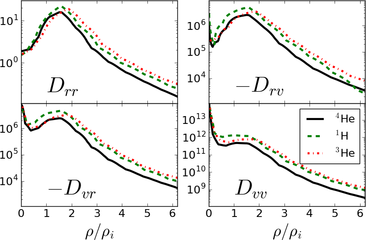
Figure 1: The diffusion coefficients of Eqs. (2) and (3) as functions of energy, for which the Larmor radius $\rho$ is used a proxy. Determined from nonlinear gs2 simulations for the three types of trace fast ions considered in this work: alpha particles (black solid), NBI knock-on hydrogen (green dashed), and ICRH-heated ³He minorities (red dotted). Units for $D_{rr}$ are $\mathrm{m}^{2}/\mathrm{s}$, $D_{rv}$ and $D_{vr}$ are given in $\mathrm{m}^{2}/\mathrm{s}^{2}$, and $D_{vv}$ in $\mathrm{m^{2}}/\mathrm{s}^{3}$.

The domain of our transport simulations is the annulus $0.1\leq r/a\leq 0.4$. Throughout this domain, the turbulence has identical properties as calculated by gyrokinetic flux tube simulations at $r=0.25a$. This is done in order to isolate the effects of transport; although a transport simulation whose flux tubes are radially-varying is more reflective of reality, and certainly possible in our framework, it is an unecessary complication. Figure 1 shows the energy dependence of the four diffusion coefficients as determined from these gs2 simulations. There, we compare several types of fast ions which might be present: ICRH-heated ³He, NBI knock-on ¹H, and fusion produced alpha particles (⁴He). The horizontal axis is expressed as the ratio of the Larmor radius (at a given energy) to the thermal hydrogen Larmor radius $\rho_{i}$. This is done to highlight the consistent physics between the species: the diffusion peaks at approximately the same Larmor radius in all cases, and has similar scaling at high energy. Although the coefficients differ by factors of order unity, qualitatively they are similar functions of energy, when properly scaled to account for different isotopes. These coefficients form the basis of the transport simulations that follow. Note that despite $D_{vr}$ and $D_{vv}$ appearing large when written in SI units, they contribute negligibly to the transport simulations because these terms are small compared to the corresponding radial transport terms and collisions. Nevertheless, these terms are retained in our simulations for completeness. For a disussion of Onsager symmetry between $D_{rv}$ and $D_{vr}$ at high energy, see the appendix.

From our gyrokinetic simulations of this case, we obtain a turbulent heat flux of $0.73\mathrm{MW}/\mathrm{m}^{2}$, which translates to about 100 MW of core heating power, which is beyond ITER’s external heating capability. This indicates that our simulations are too strongly driven. Nevertheless, we will consider this the “nominal” case, and we will routinely rescale the diffusion coefficients by various factors throughout this work to quantitatively examine the range of effect turbulence can have on fast ions. The energy dependence of the diffusion coefficients does not change significantly when more strongly- or weakly-driven turbulence simulations are run, so this practice of rescaling the diffusion coefficients is robust.

The boundary conditions used for the transport solution are as follows. At $r=0.4a$, the population of minorities is held fixed as a Maxwellian at the local ion temperature and a density of $n_{f0}=10^{17}/\mathrm{m}^{3}$, approximately 0.1% of the electron density $n_{e}=9.24\times 10^{19}/\mathrm{m}^{3}$. At the inner boundary $r=0.1a$, the net flux of minorities into the domain is zero at every energy. In velocity space, the flux through $v=0$ vanishes, and the distribution is set to vanish at a suitably high speed $v_{\mathrm{max}}$. The temperature is held fixed at $T_{e}=T_{i}=25\mathrm{keV}$ throughout the domain.

2 Comparing heated and injected ions: results and interpretation

Previous results indicated that microturbulence has the effect of causing a particle pinch of ICRH-heated minority ions against their own strong temperature gradient [2]. This conclusion was reached with a fixed fast ion distribution and radial profiles, while here we let these evolve consistently with the turbulence around the peak heating location. For comparison, we will be comparing this to ions injected at high energy, reflecting the behavior of neutral beam knock-on ions. Specifically, the velocity distribution of ICRH-type ions is more “globally” affected and moments are generally more sensitive to the turbulence, whereas for injected fast ions, turbulence has a localized effect where transport is the strongest, causing an inversion (“bump-on-tail”) in some cases.

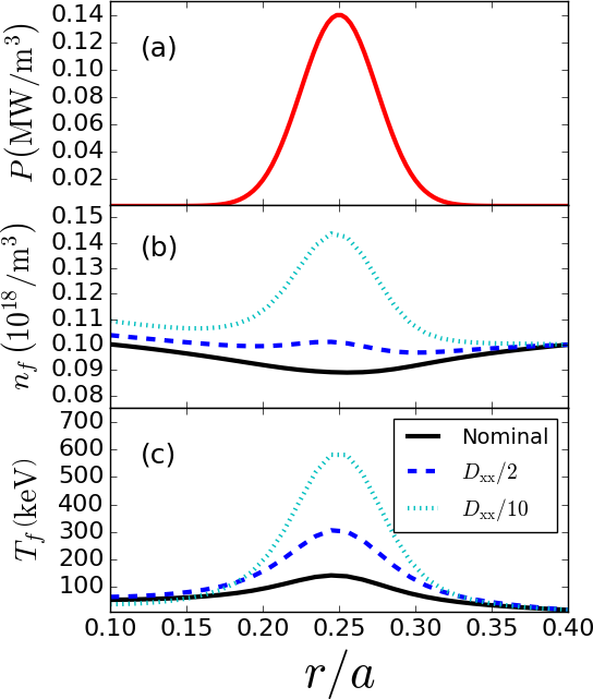
Figure 2: (a) Gaussian heat deposition profile applied in the t3core transport simulations, and the resulting (b) density, and (c) temperature profiles of the ICRH-heated ³He minority, the latter have the turbulent diffusivitives two scaled by the factors indicated.

Figure 2 shows a sample of our results, plotting the radial profile of ICRH ions as a function of radius, showing the effect of decreasing the diffusivities. Naturally, we define the temperature for a non-Maxwellian distribution as $T_{f}=\int\left(mv^{2}/3\right)F_{0}\,\mathrm{d}^{3}\mathbf{v}/n_{f}$. For sufficiently weak transport (or sufficiently strong power injection), one obtains a strong peak in temperature that depends quite strongly on the turbulence. When the turbulence is sufficiently suppressed so as to allow a sharp peak in heated minority temperature, we observe the expected density pinch. In the case of reduced turbulence, where the diffusion coefficients are scaled down by factors of ten, the density of ³He is enhanced around the heating location due to this “thermodiffusion” (a flux of particles against a temperature gradient). Eventually, particle diffusion balances this effect to create the steady-state profiles shown.

We find that the NBI-like “injected” fast ions are less sensitive to the turbulence than the ICRH ions: the peak density only changes by a factor of two when the turbulence is weakened by the same factor of ten, while the temperature changes by less than 15% (300 keV for the nominal case). We demonstrate in Fig. 3 that the peak pressure of ICRH-heated ions is more sensitive to the turbulence than NBI-type ions and, by extension, alpha particles. The latter are capable of reaching higher pressures at a given amplitude of turbulence.

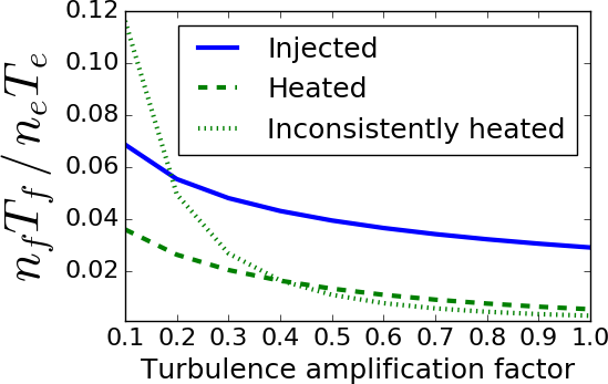
Figure 3: Maximum pressure of fast ions (normalized to the electron pressure) as a function of the turbulence amplification factor. The “inconsistently heated” case is where a constant minority density is assumed throughout the domain when implementing the heating term.

The microturbulence also has an effect on the velocity space distribution (see Fig. 4), and there again we see ICRH-heated fast ions being more sensitive. Note in Fig. 4 that, even when the turbulence is weak, it affects the velocity distribution of heated ions at all energies, while the effect on the distribution of injected ions is more localized around where $D_{rr}$ is dominant over collisions. This localization in velocity space is seen even more clearly in the distribution of alpha particles [11], which extends to yet higher energies, where it is less affected by microturbulence.

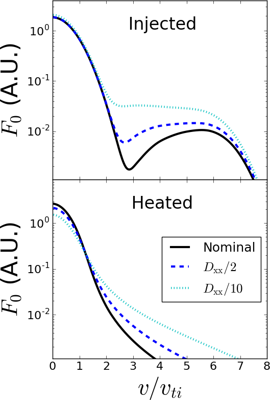
Figure 4: Modification of the distribution function of NBI-knock-ons (top) and ICRH-heated ions (bottom) at the peak heating radius $r=0.25a$. To compare with the over-driven nominal case (solid black), the diffusion coefficients are scaled down by factors of two (dashed blue) and ten (dotted cyan) in each.

To understand the physical reason for this qualitative difference, in Fig. 5 examine the paths through phase space that each type of fast ion takes. Recall that particles with moderately suprathermal energies (where $v\sim 2v_{ti}$) are most affected by the turbulence. Injected ions slow down via collisions before they reach these energies, while heated ions must “pass through” the turbulence-dominated part of velocity space before becoming part of the distribution at high energy. If the turbulence is too strong, heated particles are transported radially before reaching high energies.

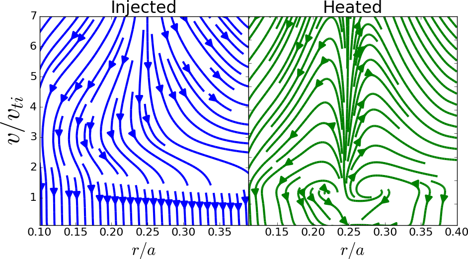
Figure 5: Stream plots showing trajectories of fast ions for the injected (left) and heated (right) case. The slope at each point is the normalized ratio $\Gamma_{v}a/\Gamma_{r}v_{ti}$. The case shown here is where the turbulence intensity is scaled down by a factor of ten. For reference, the injection energy of NBI ions is at $v_{\mathrm{inj}}\approx 6.3v_{ti}$.

3 Fast ion dilution model

The trace approximation is needed when using the diffusive form for the turbulent fluxes in Eqs. (2) and (3). However, even when fast ions are not strictly trace, they may still not participate directly in the drift wave dynamics. Instead, via quasineutrality of the equilibrium, they take the place of the thermal ions which are driving the turbulence. If this near-trace behavior can be easily predicted, one could rescale the anomalous fluxes without running additional turbulence simulations. This section seeks to develop such a model for electrostatic turbulence.

When solving for the perturbed electrostatic potential $\phi$, quasineutrality reads [14]:

$$e\phi=-\,\frac{\sum_{s}Z_{s}\int\left\langle h_{s}\right\rangle_{\mathbf{r}}\,\mathrm{d}^{3}\mathbf{v}}{\sum_{s}Z_{s}^{2}\int\left(\partial F_{0s}/\partial E\right)\,\mathrm{d}^{3}\mathbf{v}},$$ (4)

where $h_{s}$ is the non-adiabatic part of the perturbed distribution of species $s$, $F_{0s}$ is its equilibrium distribution function, and $\left\langle\right\rangle_{\mathbf{r}}$ signifies the gyro-average at fixed position in space. Suppose we have a simulation which contains only singly-charged thermal ions and adiabatic electrons in quasineutrality so that $n_{i}=n_{e}$. In this case, $e\phi\propto n_{i}/\left(n_{i}/T_{i}+n_{e}/T_{e}\right)=T_{i}/\left(1+\tau\right)$, where $\tau\equiv T_{i}/T_{e}$. Now, introduce a population of adiabatic fast ions with charge density $Z_{f}n_{f}$ such that now $n_{i}+Z_{f}n_{f}=n_{e}$. Then, $e\phi\propto n_{i}/\left(n_{i}/T_{i}+n_{e}/T_{e}+Z_{f}^{2}n_{f}/T_{f}\right)=T_{i}/\left(1+\tau_{\mathrm{eff}}\right)$ , which serves to define an “effective temperature ratio” $\tau_{\mathrm{eff}}$, and $T_{f}$ is a suitable “effective temperature” of the fast ions, which may or may not be Maxwellian. In order for the computed $\phi$ to be the same under these circumstances, we can account for the fast ions by adjusting the temperature ratio of the original simulations accordingly:

$$\tau_{\mathrm{eff}}=\left.\left(\tau+\frac{T_{i}}{T_{f}}\frac{Z_{f}^{2}n_{f}}{n_{e}}\right)\middle/\left(1-\frac{Z_{f}n_{f}}{n_{e}}\right)\right.,$$ (5)

where $\tau$ is the original (physical) temperature ratio. This second term in the numerator can be neglected for sufficiently hot ions provided that $T_{f}\gg Z_{f}T_{i}$.

The case used in this section is at $r=0.5a$ of ITER scenario 10010100 from the ITPA database [13], an ELMy H-mode case of 50/50 deuterium/tritium. The physical parameters at this flux surface are: $q=1.54$, $\hat{s}=0.435$, $\kappa=1.49$, $a\kappa^{\prime}=0.38$, $\delta=0.174$, $a\delta^{\prime}=0.44$, and a Shafranov shift derivative of $R_{0}^{\prime}(r)=-0.084$. The bulk ions are deuterium with a temperature $T_{i}=0.86T_{e}$, and nominally have $a/L_{Ti}=1.672$, while $a/L_{Te}=1.732$ and $a/L_{ne}=a/L_{ni}=0$. The fast ions are considered to be deuterium at a temperature of $T_{f}=100T_{i}$ and varying density, with no density or temperature gradients. Due to the large number of simulations required these simulations were of relatively low resolution. The spatial grid is defined by $N_{x}=N_{y}=24$, $L_{x}\approx L_{y}=10\pi\rho_{i}$ perpendicular to the magnetic field, and $N_{\theta}=18$ along the magnetic field. Velocity space has 10 points in energy, and 26 pitch angles.

Figure 6: (a) Turbulent deuterium heat flux, scanning in $a/L_{Ti}$ showing several fast ion concentrations. Dashed lines are the fitted diffusivities. (b) The thermal ion diffusivity as a function of fast ion concentration (black diamonds), a fitted (black dashed) line representing the presented model, and the dominant linear growth rate (red stars). Also shown are the results as determined from higher resolution nonlinear simulations (cyan squares).

Figure 6(a) shows the results of deuterium heat flux from nonlinear gs2 simulations near ITG marginality at several fast ion concentrations. It is evident that dilution has little effect on the critical gradient length scale: $a/L_{Ti0}\approx 1.49\pm 0.04$, but it does reduce the stiffness. The value of $\chi_{i}$ obtained for several fast ion concentrations is shown in Fig. 6(b). There, we also show that $\chi_{i}$ scales similarly to the linear growth rate, as might be expected from critical balance arguments [15]. We choose a power law fit of these simulations to reflect the behavior of Eq. (5), which results in the following model:

$$\chi_{i}\approx\chi_{i,0}\left(1-\frac{Z_{f}n_{f}}{n_{e}}\right)^{2.9},$$ (6)

where $\chi_{i,0}$ is the thermal ion diffusivity without any fast ions. Note that the experimental scaling of thermal diffusivity with respect to temperature ratio $\chi_{i}\propto\tau^{-3}$ [16] is remarkably consistent with our results when applying Eq. (5). We expect this model to be valid to the extent that the following assumptions hold: the turbulence is dominated by electrostatic dynamics; adiabatic electrons and fast ions remain a good approximation; the temperature ratio continues to obey the scaling of Ref. [16]; and one is in the limit of high “temperature” fast ions (i.e. the fast ion term vanishes in the denominator of Eq. (4)). These latter two assumptions can be relaxed by replacing the power in Eq. (6) and/or by including the additional term in the numerator of Eq. (5). Furthermore, we note that previous work done on fast ion dilution [17, 4] is also consistent with this model.

By applying Eq. (6), a transport simulation of the bulk plasma can easily and consistently respond to the stabilizing presence of fast ions, at least to a leading approximation. This could have implications for the formation of internal transport barriers, and the intrepid modeller can optimise the heating profile to take advantage of this effect.

Conclusion

In this work, we explored the global non-Maxwellian transport of isotropic heated minority ions, allowing their radial and velocity distribution to arise naturally from the physics of collisions, gyrokinetic microturbulence, and direct heating. Our aim was to highlight the qualitative differences between their response to microturbulence and that of fast ions such as those generated by NBI or fusion reactions. Despite their very similar diffusion coefficients, these differences fundamentally limit how robustly they can mimic the turbulent transport of alpha particles, and this limitation is primarily due to how each type gains energy. However, their relatively strong sensitivity could allow them to be a useful probe of the turbulence, and as experimental validation for transport tools such as t3core.

It has been experimentally observed that simultaneously applying NBI and IRCH heating simultaneously results in more heating than the sum of either of them alone [18]. Our results provide a possible explanation for this phenomenon. ICRH-heated minorities are more affected by the turbulence because they have the opportunity to transport radially before being heated. Therefore, if one heats ions via ICRH that are already at high energy (via, for example, NBI), where turbulence has less effect, then one avoids the strong-transport region of phase space altogether.

Two important caveats to our results are the electrostatic and isotropic assumptions. Electromagnetic fluctuations, even in primarily electrostatic turbulence, could be important for trace transport at sufficiently high plasma beta. Also, the fast ions considered here are generally not isotropic in velocity space. In order for our results to faithfully reflect the isotropic part of such a velocity distribution, we had to ignore the pitch-angle dependence of the turbulent diffusion coefficients. We believe that our core result (that ICRH ions are more sensitive to the microturbulence, having an impact on the distribution at all energies) is robust to relaxing this assumption, but further study is expected and welcome.

The transport results presented here rely upon fast ions being trace, which is a robust assumption for electrostatic turbulence at small concentrations. Where fast ions might make up a more significant fraction of the plasma, we presented a model to account for their effect on the bulk plasma transport as a next approximation. Although the t3core simulations presented here do not employ this model, we believe it will be very useful for future transport simulations.

The authors would like to thank Yevgen Kazakov for the original inspiration of high-energy heated minority and Torbjörn Hellsten for helpful discussion. Simulations were performed on the SNIC cluster Hebbe (project nr. SNIC2016-1-161) and the NERSC supercomputer Edison. This work was supported by the Framework grant for Strategic Energy Research (Dnr. 2014-5392) from Vetenskapsrådet, the International Career Grant (Dnr. 330-2014-6313), and the U.S. Department of Energy Office of Fusion Energy Science (DEFG0293ER54197 and DEFC0208ER54964).

Appendix A Onsager symmetry for quasilinear phase space transport

The astute reader might notice a type of Onsager symmetry between $D_{rv}$ and $D_{vr}$ at high energy in Fig. 1. A proof of Onsager symmetry for quasilinear radial transport of a Maxwellian species has already been shown [19], but this is not the case for nonlinear turbulence [20]. In this appendix, we’ll show that this symmetry holds for quasilinear transport even in $r$-$v$ phase space, as has been observed here and elsewhere [5]. This is more than coincidence, and here we show that this is rigorous as long as the magnetic drift velocity is dominant over the nonlinear drift velocity in the gyrokinetic equation.

The operator $\mathcal{L}$ is the left-hand side of the collisionless gyrokinetic equation, so that when acting on the non-adiabatic perturbed distribution $h$:

$$\mathcal{L}\left[h\right]\equiv\frac{\partial h}{\partial t}+\left(v_{\|}\mathbf{b}+\mathbf{v_{d}}+\mathbf{v}_{\phi}\right)\cdot\nabla h,$$ (7)

where $\mathbf{v}_{d}$ is the magnetic drift velocity including the $\nabla B$ and curvature drifts, and $\mathbf{v}_{\phi}\equiv\left(c/B\right)\mathbf{b}\times\nabla\left\langle\phi\right\rangle_{\mathbf{R}}$. The unit vector $\mathbf{b}$ points in the direction of the equilibrium magnetic field.

What makes our transport calculations possible is that, for a trace species only, $\mathcal{L}$ is a linear operator, although it does in general depend on $\phi$. Note that this is not equivalent to the quasilinear approximation used, for example, in Refs. [3] and [5], and is more generally applicable. The quasilinear approximation is when one further assumes that the $\mathbf{v}_{\phi}$ term in Eq. 7 is negligible. This becomes more accurate at high energy, when $\mathbf{v}_{d}\gg\mathbf{v}_{\phi}$.

Now, consider the following expressions for the diffusion coefficients:

$$D_{rr}=\left\langle\sum_{\sigma_{\|}}\int\mathcal{L}^{-1}\left[\mathbf{v}_{\phi}\cdot\nabla r\right]\left(\mathbf{v}_{\phi}\cdot\nabla r\right)\mathcal{J}_{v}\mathrm{d}\lambda\right\rangle_{t}$$ (8)

$$D_{rv}=\left\langle\sum_{\sigma_{\|}}\int\mathcal{L}^{-1}\left[\frac{\partial\left\langle\phi\right\rangle_{\mathbf{R}}}{\partial t}\right]\frac{Ze}{mv}\left(\mathbf{v}_{\phi}\cdot\nabla r\right)\mathcal{J}_{v}\mathrm{d}\lambda\right\rangle_{t}$$ (9)

$$D_{vr}=\left\langle\sum_{\sigma_{\|}}\int\mathcal{L}^{-1}\left[\mathbf{v}_{\phi}\cdot\nabla r\right]\frac{Ze}{mv}\left(\frac{\partial\left\langle\phi\right\rangle_{\mathbf{R}}}{\partial t}\right)\mathcal{J}_{v}\mathrm{d}\lambda\right\rangle_{t}$$ (10)

$$D_{vv}=\left\langle\sum_{\sigma_{\|}}\int\mathcal{L}^{-1}\left[\frac{\partial\left\langle\phi\right\rangle_{\mathbf{R}}}{\partial t}\right]\frac{Z^{2}e^{2}}{m^{2}v^{2}}\left(\frac{\partial\left\langle\phi\right\rangle_{\mathbf{R}}}{\partial t}\right)\mathcal{J}_{v}\mathrm{d}\lambda\right\rangle_{t}.$$ (11)

Here, $\mathcal{J}_{v}$ is the velocity space Jacobian for coordinates $v$ and $\lambda=v_{\perp}^{2}/v^{2}$, $\sigma_{\|}$ is the sign of the parallel velocity (which would otherwise ambiguous in these coordinates), and $\left\langle\right\rangle_{t}$ represents a time-average and a spatial average over the flux-tube. Consider the off-diagonal terms defined in Eqs. 9 and 10. If we assume that $\mathcal{L}$ does not depend on $\phi$ (thus has no explicit time dependence), then we can show that $D_{rv}=D_{vr}$ by Fourier transforming in time. For convenience, let $\mathcal{D}\equiv\mathcal{L}-\partial/\partial t$. Recalling the definition of time average to be an integral over time:

$$\int\mathcal{L}^{-1}\left[\mathbf{v}_{\phi}(t)\cdot\nabla r\right]\frac{\partial\left\langle\phi\right\rangle_{\mathbf{R}}}{\partial t}\,dt$$ (12)

$$=\int\frac{\partial\left\langle\phi\right\rangle_{\mathbf{R}}}{\partial t}\int\,\tilde{\mathcal{L}}^{-1}\left[\mathbf{v}_{\phi}(t)\cdot\nabla r\right]\left(\omega\right)e^{i\omega t}d\omega\,\,dt$$ (13)

$$=\int\frac{\partial\left\langle\phi\right\rangle_{\mathbf{R}}}{\partial t}\int\,\frac{\tilde{\mathbf{v}}_{\phi}(\omega)\cdot\nabla r}{-i\omega+\mathcal{D}}e^{i\omega t}\,d\omega\,dt$$ (14)

$$=\int\int\int\frac{\partial\left\langle\phi\right\rangle_{\mathbf{R}}}{\partial t}\,\frac{\mathbf{v}_{\phi}(t^{\prime})\cdot\nabla r}{-i\omega+\mathcal{D}}e^{i\omega\left(t-t^{\prime}\right)}\,dt^{\prime}\,d\omega\,dt$$ (15)

$$=\int\int\int\mathbf{v}_{\phi}(t)\cdot\nabla r\frac{\partial\left\langle\phi\right\rangle_{\mathbf{R}}/\partial t^{\prime}}{-i\omega+\mathcal{D}}e^{i\omega\left(t^{\prime}-t\right)}\,dt^{\prime}\,d\omega\,dt$$ (16)

$$=\int\mathcal{L}^{-1}\left[\frac{\partial\left\langle\phi\right\rangle_{\mathbf{R}}}{\partial t^{\prime}}\right]\mathbf{v}_{\phi}(t^{\prime})\cdot\nabla r\,dt^{\prime},$$ (17)

which shows that Eqs. 9 and 10 are equivalent. The key approximation was that $\mathcal{D}$ does not depend on time, which is the case for the quasilinear approximation. Therefore, while not generally applicable in nonlinear turbulence, Onsager symmetry is expected at high energy to the extent that $\mathbf{v}_{\phi}\ll\mathbf{v}_{d}$.

References

References

- [1] Ye.O. Kazakov, D. Van Eester, R. Dumont, and J. Ongena. On resonant ICRF absorption in three-ion component plasmas: a new promising tool for fast ion generation. Nuclear Fusion, 55(3):032001, March 2015.
- [2] István Pusztai, George J Wilkie, Yevgen O Kazakov, and Tünde Fülöp. Turbulent transport of MeV range cyclotron heated minorities as compared to alpha particles. Plasma Physics and Controlled Fusion, 58(10):105001, November 2016.
- [3] C. Angioni and A. G. Peeters. Gyrokinetic calculations of diffusive and convective transport of particles with a slowing-down distribution function. Physics of Plasmas, 15(5):052307, 2008.
- [4] G. J. Wilkie. Microturbulent transport of non-Maxwellian alpha particles. PhD thesis, University of Maryland, 2015.
- [5] R. E. Waltz, E. M. Bass, and G. M. Staebler. Quasilinear model for energetic particle diffusion in radial and velocity space. Physics of Plasmas, 20(4):042510, 2013.
- [6] T. Hauff, M. J. Pueschel, T. Dannert, and F. Jenko. Electrostatic and magnetic transport of energetic ions in turbulent plasmas. Physical Review Letters, 102(7), February 2009.
- [7] M.J. Pueschel, F. Jenko, M. Schneller, T. Hauff, S. Günter, and G. Tardini. Anomalous diffusion of energetic particles: connecting experiment and simulations. Nuclear Fusion, 52(10):103018, October 2012.
- [8] G. J. Wilkie, I. G. Abel, E. G. Highcock, and W. Dorland. Validating modeling assumptions of alpha particles in electrostatic turbulence. Journal of Plasma Physics, 81(03):905810306, 2015.
- [9] P. Helander and D. Sigmar. Collisional Transport in Magnetized Plasmas. Cambridge University Press, Cambridge, 2002.
- [10] Thomas Howard Stix. Fast-wave heating of a two-component plasma. Nuclear Fusion, 15(5):737, 1975.
- [11] G. J. Wilkie, I. G. Abel, M. Landreman, and W. Dorland. Transport and deceleration of fusion products in microturbulence. Physics of Plasmas, 23(6):060703, June 2016.
- [12] W. Dorland, F. Jenko, M. Kotschenreuther, and B. N. Rogers. Electron Temperature Gradient Turbulence. Physical Review Letters, 85(26):5597, 2000.
- [13] C.M. Roach, M. Walters, R.V. Budny, F. Imbeaux, T.W. Fredian, M. Greenwald, J.A. Stillerman, D.A. Alexander, J. Carlsson, J.R. Cary, F. Ryter, J. Stober, P. Gohil, C. Greenfield, M. Murakami, G. Bracco, B. Esposito, M. Romanelli, V. Parail, P. Stubberfield, I. Voitsekhovitch, C. Brickley, A.R. Field, Y. Sakamoto, T. Fujita, T. Fukuda, N. Hayashi, G.M.D Hogeweij, A. Chudnovskiy, N.A. Kinerva, C.E. Kessel, T. Aniel, G.T. Hoang, J. Ongena, E.J. Doyle, W.A. Houlberg, A.R. Polevoi, ITPA Confinement Database and Modelling Topical Group, and ITPA Transport Physics Topical Group. The 2008 Public Release of the International Multi-tokamak Confinement Profile Database. Nuclear Fusion, 48(12):125001, December 2008.
- [14] I G Abel, G G Plunk, E Wang, M Barnes, S C Cowley, W Dorland, and A A Schekochihin. Multiscale gyrokinetics for rotating tokamak plasmas: fluctuations, transport and energy flows. Reports on Progress in Physics, 76(11):116201, November 2013.
- [15] M. Barnes, F. I. Parra, and A. A. Schekochihin. Critically Balanced Ion Temperature Gradient Turbulence in Fusion Plasmas. Physical Review Letters, 107(11), September 2011.
- [16] C. C. Petty, M. R. Wade, J. E. Kinsey, R. J. Groebner, T. C. Luce, and G. M. Staebler. Dependence of heat and particle transport on the ratio of the ion and electron temperatures. Physical review letters, 83(18):3661, 1999.
- [17] G Tardini, J Hobirk, V.G Igochine, C.F Maggi, P Martin, D McCune, A.G Peeters, A.C.C Sips, A Stäbler, J Stober, and the ASDEX Upgrade Team. Thermal ions dilution and ITG suppression in ASDEX Upgrade ion ITBs. Nuclear Fusion, 47(4):280–287, April 2007.
- [18] A V Krasilnikov, D Van Eester, E Lerche, J Ongena, V N Amosov, T Biewer, G Bonheure, K Crombe, G Ericsson, B Esposito, L Giacomelli, C Hellesen, A Hjalmarsson, S Jachmich, J Kallne, Yu A Kaschuck, V Kiptily, H Leggate, J Mailloux, D Marocco, M-L Mayoral, S Popovichev, M Riva, M Santala, M Stamp, V Vdovin, A Walden, and JET EFDA Task Force Heating and JET EFDA contributors. Fundamental ion cyclotron resonance heating of JET deuterium plasmas. Plasma Physics and Controlled Fusion, 51(4):044005, April 2009.
- [19] H. Sugama, M. Okamoto, W. Horton, and M. Wakatani. Transport processes and entropy production in toroidal plasmas with gyrokinetic electromagnetic turbulence. Physics of Plasmas, 3(6):2379, 1996.
- [20] R. Balescu. Is Onsager symmetry relevant in the transport equations for magnetically confined plasmas? Physics of Fluids B: Plasma Physics, 3(3):564, 1991.