“Sampling” as a Baseline Optimizer for Search-based Software Engineering

Abstract

Increasingly, Software Engineering (SE) researchers use search-based optimization techniques to solve SE problems with multiple conflicting objectives. These techniques often apply CPU-intensive evolutionary algorithms to explore generations of mutations to a population of candidate solutions. An alternative approach, proposed in this paper, is to start with a very large population and sample down to just the better solutions. We call this method “Sway ”, short for “the sampling way”. This paper compares Sway versus state-of-the-art search-based SE tools using seven models: five software product line models; and two other software process control models (concerned with project management, effort estimation, and selection of requirements) during incremental agile development. For these models, the experiments of this paper show that Sway is competitive with corresponding state-of-the-art evolutionary algorithms while requiring orders of magnitude fewer evaluations. Considering the simplicity and effectiveness of Sway , we, therefore, propose this approach as a baseline method for search-based software engineering models, especially for models that are very slow to execute.

1 Introduction

Software engineers often need to answer questions that explore trade-offs between competing goals. For example:

1. What is the smallest set of test cases that cover all program branches?

2. What is the set of requirements that balances software development cost and customer satisfaction?

3. What sequence of refactoring steps take the least effort while most decreasing the future maintenance costs of a system?

SBSE, or search-based software engineering, is a commonly-used technique for solving such problems. Two things are required for using SBSE methods:

• The model is some device which, if its inputs are perturbed, generates multiple outputs (one for each objective).

• The optimizer is the a device that experiments with different model inputs to improve model outputs.

Different models can require different optimizers. According to Wolpert & Macready [72], no single algorithm can ever be best for all optimization problems. They caution that for every class of problem where algorithm $A$ performs best, there is some other class of problems where $A$ will perform poorly. Hence, when commissioning a new domain, there is always the need for some experimentation to match the particulars of the local model to particular algorithms.

When conducting such commissioning experiments, it is very useful to have a baseline optimizer; i.e., an algorithm which can generate floor performance values. Such baselines let a developer quickly rule out any optimization option that falls “below the floor”. In this way, researchers and industrial practitioners can achieve fast early results, while also gaining some guidance in all their subsequent experimentation (specifically: “try to beat the baseline”).

This paper proposes a new algorithm called Sway (short for the sampling way) as a baseline optimizer for search-based SE problems. As described in the next section, Sway has all the properties desirable for a baseline method such as simplicity of implementation and fast execution times. Further, the experiments of this paper show that Sway usually performs as well as, or better than, more complex algorithms even for some very hard problems (e.g., selecting candidate products according to five objectives from highly constrained product lines). Most importantly, Sway adds very little to the overall effort required to study a new problem. For example, we tested Sway in three different SE problems: 1) reducing risk, defects as well as development efforts of a project, 2) optimizing agile project structures, and 3) utilizing software product line model to find out features to develop in requirement engineering. For all models, Sway ’s median cost was just 3% of runtimes and 1% of the number of model evaluations (compared to only running the standard optimizers).

The rest of this paper is structured as follows: The remainder of this section will introduce our prior work and main contributions of this paper. Section 2 briefly introduces the background of SBSE and evolutionary algorithms. Section 3 shows the core algorithms of Sway. In Section 4, Sway is applied on above three SE case studies. Results from these case studies are discussed in Section 5. After that, the rest of the paper explores threats to validity, reviews some more related work.

The conclusion of this paper is not that Sway is always the best choice optimizing SBSE models. Rather, since Sway is so simple and so fast, it is a reasonable first choice for benchmarking other approaches. To aid in that benchmarking process, all our scripts and sample problems are available online in Github. Also, to simplify all future references to this material, the same content has been assigned a digital object identifier in a public-domain repository.

1.1 Relation to Prior Work

This paper significantly extends prior work of the authors. In 2014, Krall & Menzies proposed GALE [36, 35, 37] that solved multi-objective problems via a combination of methods. A subsequent report [64] found that GALE needlessly over-elaborated some aspects of its design. That subsequent report evaluated a preliminary version of Sway using results from two similar models, XOMO and POM3 models, both of whose decision representation are a continuous numeric array. That subsequent the report was expanded into a journal article [13] to explore a lightly constrained model for Next Release Problem (NRP). This current paper began when it was realized that the methods used in that journal article failed when applied to heavily constrained models and models with binary decisions.

In heavily constrained models, a naive “generate-at-random” strategy results in too few candidate solutions. Accordingly, this paper processes heavily constrained models using an SAT solver to generate the initial population.

Our prior versions of Sway used various heuristics to divide the space of candidates– all of which fail for models with binary decision variables. The reason for this is simple: numeric decisions tend to spread candidates all over the $D$-dimensional space containing the $D$ decisions. However, for $D$ binary decisions, all the candidates fall to the vertexes of the $D$-dimensional decision space. Hence, Sway was failing when it kept proposing useless divisions of the empty space between the vertices. Accordingly, to distribute the candidates containing binary decisions, this paper uses a novel coordinate system. In that coordinate system, initial candidates are first divided by problem-specific heuristics, then grouped by similarities.

Another important distinctive feature of this paper is its evaluation methodology. In this paper, when evaluating the performance of Sway on our models, we took care to compare against demonstrably state-of-the-art alternatives. For example, we do not use the default settings of the NSGA-II [17] optimizer but instead, apply an extensive grid search operation to find better settings.

Overall, the unique contributions of this paper are:

1. A new baseline approach to multi-objective optimization;

2. Two forms of this new approach: one for continuous variables and another one for discrete variables (this discrete version of Sway has not been published before);

3. Results are evaluated by more metrics (Generational Distance, Generated Spread, Pareto Front Size, and Hypervolume);

4. Results are compared against state-of-the-art or highly-tuned algorithms;

5. Case studies show that Sway allows for a very rapid processing of complex and large heavily constrained models;

6. Defining an executable method for baselining new SBSE methods. To allow ready access to that method, our scripts and sample problems are available online for free download.

2 Background

2.1 Baselining with Sway 

Experienced researchers endorse the use of baseline algorithms. For example, in his textbook on Empirical Methods for AI, Cohen [16] strongly advocates comparing supposedly sophisticated systems against simpler alternatives. In the machine learning community, Hotle [32] uses the OneR baseline algorithm as a scout that runs ahead of a more complicated learner as a way to judge the complexity of up-coming tasks. In the software engineering community, Whigham et al. [71] recently proposed baseline methods for effort estimation (for other baseline methods in effort estimation, see Mittas et al. [48]). Shepperd and Macdonnel [62] argue convincingly that measurements are best viewed as ratios compared to measurements taken from some minimal baseline system. Work on cross versus within-company cost estimation has also recommended the use of some very simple baseline (they recommend regression as their default model) [33].

In their recent article on baselines in software engineering, Whigham et al. [71] propose guidelines for designing a baseline implementation that include:

1. Be simple to describe and implement;

2. Be applicable to a range of models;

3. Be publicly available via a reference implementation and associated environment for execution;

To their criteria, we would add that for multi-objective optimization algorithms, such baselines should also:

1. Offer comparable performance to standard methods. While we do not expect a baseline method to out-perform all state-of-the-art methods, for a baseline to be insightful, it needs to offer a level of performance that often approaches the state-of-the-art.

2. Not be resource expensive to apply (measured in terms of required CPU or number of evaluations). The resources required to reach a decision are not a major concern for Whigham’s cost estimation work. Before a community adopts SBSE baseline methods, we must first ensure that baseline executes very quickly. Some search-based software engineering methods can require days to years of CPU-time to terminate [70]. Hence, unlike Whigham et al., we take care not to select baseline methods that are impractically slow.

Sway satisfies all the above criteria. The method is straightforward:

• Generate a very large population of random candidates;

• Evaluate a small number of representative candidates (using the methods described in §3);

• Cull any candidates that are near the poorly performing representatives.

Note that this uses much less machinery than a standard genetic algorithm; i.e., there are no complex selection, mutation or crossover operators. Nor does Sway employ multi-generational reasoning. As a result, it is a simple matter to code Sway (see pseudocode in Algorithm 1).

As to being applicable to a wide range of models, in this paper we apply Sway to models with boolean and continuous decision variables:

• Our models with continuous decision variables are XOMO and POM3. XOMO [44, 47, 46] is an SE model where the optimization task is to reduce the defects, risk, development months, and the total number of staff members associated with a software project. POM3 [10, 56, 8] is an SE model of agile development towards negotiating what tasks to do next within a team.

• Our model with boolean decision variables is software product lines [58, 59] for which the optimization task is to extract (a) valid products that (b) have more features and use (c) the most familiar features that (d) costs the least to implement and which (e) has the fewest known bugs.

As to public availability, a full implementation of Sway including all the case studies presented here (including working implementations of other multi-objective evolutionary algorithms and our evaluation models in [64]) is available online.

In terms of comparative performance, for each model, we compared Sway ’s performance against the established state-of-the-art method as reported in the literature. In those comparative results, Sway was usually as good, and sometimes even a little better, than the state-of-the-art.

Sway is also not resource expensive to apply. The algorithm does not evaluate all of its random candidates. Instead, Sway employs a top-down bi-cluster procedure that finds two distant points $X,Y$, then labels all points according to which of $X,Y$ they are closest to. The points are then evaluated, and all points near the worst one are culled. Hence, Sway only evaluates $log(N)$ of $N$ candidates, which makes it a relatively very fast algorithm:

• Measured in terms of addition model evaluations, collecting baseline results from Sway would require $\{1,1,1,2,2,6,6,9,33\}\%$ additional evaluations in various models.

• Measured in terms of total runtime, Sway adds $\{1,1,1,1,1,1,2,2,3\}\%$ to the runtime of other optimizers.

Note that in the above, values less than 100 denote evaluations that are fewer and hence better than other methods. Note also that, usually, Sway terminates very quickly.

This reduction in runtime is an important feature of Sway since some optimization studies can be very CPU intensive. For example, recent MOEA studies in software engineering by Fu et al. [26] and Wang et al. [70] required 22 days and 15 years of CPU time respectively. While, to some extent, this high CPU cost can be managed via the use of cloud computing services, those computing environments are extensively monetized so the total financial cost of tuning can be prohibitive. We note that all that money is a wasted resource if there is a more straightforward way (e.g., Sway ) to achieve similar results.

Sway offers many benefits to practitioners and researchers:

1. Researchers can use results of Sway as the “sanity checker”. Experiments showed that results of Sway are much better than random configurations and in most times, it is comparable to standard optimizers. Consequently, when designing new optimizers, researchers can compare their results to Sway ’s to see whether their superiority is significant.

2. Practitioners can use Sway to get quick feedback on their adjustments. For example, in agile development, managers can apply Sway to POM3 to quickly get approximate changes of developing efforts or costs when they adjust release plans or team personnel, etc.

2.2 Search Based Software Engineering (SBSE)

Sway is our proposed baseline algorithm for search-based software engineering (SBSE). This section reviews the field of SBSE.

Throughout the software engineering life cycle, from requirement engineering, project planning to software testing, maintenance, and re-engineering, software engineers need to find a balance between different goals such as:

• Software product line optimization: Sayyad et. al. [59] compared several MOEAs, including SPEA2, IBEA, NSGA-II[17], etc, and found that IBEA algorithm performed best in generating valid products from product line descriptions (for details see §4.1.3).

• Project planning: Ferrucci et al. [23, 57] modified the crossover operator in the NSGA-II algorithm and found that their approach (called NSGA-II_v) was useful for planning how to make the best use of project overtime.

• Test suite minimization: Wang et al.[68] showed that their “weighted-based” genetic algorithm significantly outperformed other methods using industrial case study for Cisco Systems.

• Improving defect prediction: Fu et al. [26] and Harman et at. [27] report that software quality predictors learned from data miners can be improved if an evolutionary algorithm first adjusts the tuning parameters of the learner.

• Software clone detectors: Wang, Harman et al. [70] report that the arduous task of configuring complex analysis tools like software clone detectors can be automated via multi-objective evolutionary algorithms.

All of these problems can be viewed as optimization problems; i.e., tune the configuration parameters of a model such that, when that model runs, it generates “good” outputs (i.e., output demonstrably better than other possible outputs). Given the complexities of software engineering, SE models are often too complicated to prove that output is optimal. For such models, the best we can do is run multiple optimizers and report the best output seen across all those optimizers. In the past, due to the simplicity of software structure, developers/experts could make a decision based on their empirical knowledge. For such models of such simple knowledge, it may have been possible to demand that those outputs are “optimal”; i.e., there exists no other configuration such that a better output can be generated. However, modern software is becoming increasingly complex. Finding the optimal solution to such kind of problems may be difficult/impossible. For example, in a project staffing problem, if there are ten experts available and 10 activities to be accomplished, the total number of available combinations is 10 billion ($10^{10}$). For such large search spaces, exhaustively enumerating and assessing all possibilities is impractical.

When brute force methods fail, it is possible to employ Metaheuristic search algorithms to explore complex models. The Search Based Software Engineering (SBSE)’s favorite meta-heuristic search algorithms are evolutionary algorithms [31]. Such algorithms offer “a higher-level procedure or heuristic designed to find, generate, or select a heuristic (partial search algorithm) that may provide a sufficiently good solution to an optimization/search problem, especially with incomplete or imperfect information or limited computation capacity” [7]. As seen in Figure 1, within the research community, this has become a very popular approach.

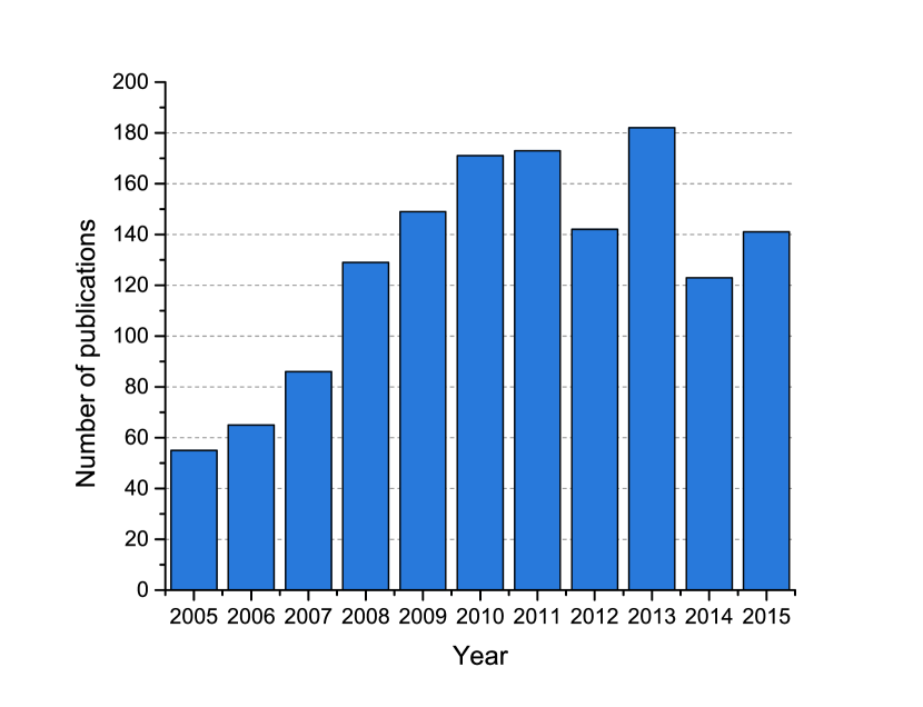
Figure 1: SBSE publications. From [74]

One advantage of these meta-heuristic algorithms is that they can simultaneously explore multiple goals at the same time. The next section of this paper introduces multi-objective evolutionary optimization algorithms, which are widely used in SBSE.

2.3 Multi-Objective Evolutionary Algorithms (MOEA)

In SBSE, the software engineering problem is treated as a mathematical model: given the numeric (or boolean) configurations/decisions variables, the model should return one or more objectives. In a nutshell, the model can convert decisions “d” into objective scores “o”, i.e.

o = model(d) (1)

The direction of optimization for the objectives can be to either maximize or minimize their values. For example, in software engineering, we might want to maximize the delivered functionality while also minimizing the cost to make that delivery. If model delivers just one objective, then we call the this a single-objective optimization problem. On the other hand, when there are many objectives we call that a multi-objective optimization problem.

For the multi-objective optimization problem, often there is no “$d$” which can minimize (or maximize) all objectives. Rather, the “best” $d$ offers a good trade-off between competing objectives. In such a space of competing goals, we cannot be optimal on all objectives, simultaneously. Rather, we must seek a Pareto frontier or solution of multiple solutions where no other solutions in the frontier “dominate” any other [77].

There are two types of dominance– binary dominance and continuous dominance. Binary dominance is defined as follows: solution $x$ is said to binary dominate the solution $y$ if and only if the objectives in $x$ is partially less (larger when the corresponding objective is to maximize) than the objectives in $y$, that is,

$\forall o\in\textit{obj }o_{x}\succeq o_{y}\text{ and }\exists o\in\textit{obj }o_{x}\succ o_{y}$

where obj are the objectives and ($\succeq,\succ$) tests if an objective score in one individual is (no worse, better) than the other. Continuous dominance [76], favors $x$ over $y$ if $x$ “losses” least:

$$\begin{array}[]{rcl}x\succ y&=&\textit{loss}(y,x)>\textit{loss}(x,y)\\ \textit{loss}(x,y)&=&\sum_{j}^{n}-e^{\Delta(j,x,y,n)}/n\\ \Delta(j,x,y,n)&=&w_{j}(o_{j,x}-o_{j,y})/n\end{array}$$ (2)

MOEAs create the initial population first, and then execute the crossover and mutation repeatedly until “tired or happy”; i.e., until we have run out of CPU time limitation or until we have reached solutions that suffice for the purposes at hand. The basic framework for MOEAs is as follows:

1. Generate generation 0 using some initialization policy

2. Evaluate all individuals in generation 0

3. Repeat until tired or happy

   1. Cross-over items in current generation to make new population;

   2. Mutate population by making small changes;

   3. Evaluate individuals in the population;

   4. Select some elite subset of the population to form a new generation.

One simple way to understand MOEAs is to compare them with Darwin’s theory of evolution. To find good scores for the objectives, start from a group of individuals. As time goes by, the individuals inside the group crossover. The offspring which have better fitness scores tend to survive (in the selection step). During the evolution, the mutation operation can increase the diversity of the group and avoid the evolution from getting trapped in the local optimal.

Standard MOEA algorithms might be not suitable for some SE models. For example, the standard initiation operator is to build members of the population by selecting, at random, across the range of all known decisions. However, this may not be the best procedure for all models. For example:

• Sayyad et al. found that the best way to seed a population for a five-goal optimization problem was to first run a two-goal optimizer (for the hardest pair of goals), then use the two-goal optimizer as input to the five-goal optimizer [58].

• Later in this paper (§4.1.3), we will use a case-study of optimizing a heavily constrained model. For that case study, only three out of 10,000 randomly generated candidates satisfied the constraints of that model. Hence, for that model, Sway uses an SAT-solver to initialize the space of candidates.

There are many cross-over and mutation operators, such as one/two point(s) cross-over, Gaussian mutation, FlipBit mutation, uniform partially matched crossover (UPMX) [15], etc. Specific domains might require specialized cross-over operators. For example, for program repair, [50] created a new cross-over operator, Unif1Space which improved the fix rate by 34%.

When exploring new MOEAs, much attention has been paid to the selection operator. For example, the core innovation in NSGA-II [18] is its method of performing the selection. Candidates are sorted heuristically into bands according to how many other candidates they dominate. The top $B$ bands containing some desired number $N$ candidates survive to the next generation. If these $B$ bands contain more than $N$ candidates, then:

• NSGA-II sorts candidates by each objective $o_{x}$.

• Next, NSGA-II annotates each candidate $y$ with the gap $g_{o}^{y}$ to its nearest neighbors within the sort of objective $o$, where $o(x)<o_{x}(y)<o(z)$ and $g_{o}^{y}=o(z)-o(x)$

• The crowding-distance $D$ around a candidate $y$ is a hyper-rectangle with volume $D_{y}=\prod_{o\in\textit{obj }}g_{o}^{y}$.

• NSGA-II sorts the candidates $D_{y}$ in the last band, then selects the candidates from the least crowded regions.

The rationale for this select rule is as follows. In crowded regions, we can reject some candidates while still retaining many others. However, in order to retain the shape of the Pareto frontier, it is important to retain candidates from the less-crowded regions.

As to the evaluation operator, the standard approach is, for each decision, run the underlying model to generate objective scores for those decisions. Such an evaluation operator may be too cumbersome for many reasons:

• Verrappa and Letier warn that “..for industrial problems, these algorithms generate (many) solutions, which makes the tasks of understanding them and selecting one among them difficult and time-consuming” [65].

• Zuluaga et al. comment on the cost of evaluating all decisions for their models of software/hardware co-design: “synthesis of only one design can take hours or even days.”  [78].

• Harman comments on the problems of evolving a test suite for software: if every candidate solution requires a time-consuming execution of the entire system: such test suite generation can take weeks of execution time [73].

• Krall & Menzies explored the optimization of complex NASA models of air traffic control. After discussing the simulation needs of NASA’s research scientists, they concluded that those models would take three months to execute, even utilizing NASA’s supercomputers [36].

Hence, Sway’s evaluation operator strives to reduce the number of requested model evaluation. To achieve this goal, Sway applies a sampling technique (discussed in §3) that reduces the number of model evaluations and, hence, the total running time.

3 Sway : The Sampling WAY

This section introduces our method Sway that recursively clusters the candidates in order to isolate the superior cluster. Unlike the common MOEA algorithms (where candidates are improved by multiple generations of mutation, crossover, and selection), Sway just selects a small superior set candidates among a group of candidates. Consequently, the first step of Sway is to generate a huge amount of candidates. We generated 10,000 in our experiments.

If we cluster the candidates through their objectives, we need to evaluate all candidates (just like common MOEA algorithms), Sway would be very slow, since model evaluations in many SE problems are extremely time-consuming (see §2.2). Instead, the Sway clusters the candidates by their decisions (recall that decisions and objectives were distinguished in §2.3 Equation 1).

Implicit in decision clustering is the assumption that there exists a close association between the genotype (decision) and phenotype objective) spaces. In SE, this is not an unwarranted assumption. For example, cloud environment configuration meets such requirement– an improved number of VM/memories can lead to better quality service  [3]. Also, in the POM3, XOMO model and software product line model (see §4.1), Sway worked satisfactorily suggesting that at least models have a closely associated genotype/phenotype spaces.

Input : items – The candidates

Output : pruned results

Parameter : enough – The minimum cluster size

Require Func :  Split, see §3.1, §3.2

Better, see §3.3

1

2if numberOf(items) ¡ enough then

3       return items

4      

5 else

6       $\Delta_{1},\Delta_{2}\leftarrow\emptyset,\emptyset$

7       [west, east], [westItems, eastItems] $\leftarrow$ Split(items)

8       if $\neg$Better(west, east) then  $\Delta_{1}\leftarrow$ Sway (eastItems)

9       if $\neg$Better(east, west) then  $\Delta_{2}\leftarrow$ Sway(westItems)

10       return $\Delta_{1}+\Delta_{2}$

11

Algorithm 1 Sway 

Algorithm 1 shows the general framework of Sway. The candidates are split into two parts according to their decisions. Then Sway prunes half of them based on the objectives of the corresponding representatives, where the limited number of model evaluations come from. The Split function may differ for different types of decision representation and we will discuss the Split function very soon:

• If the population size is smaller than some threshold, then we just return all candidates (line 1). Otherwise, Sway splits the candidates into two parts, “west side” and the “east side.”

• After that, lines 6 and 7 compare representatives of the sides. Sway uses different methods to find those representatives– see §3.1 and 3.2.

• Prune the candidates based on a comparison of the representatives. If neither representative is better, then we Sway on each part.

Sway is a divide-and-conquer process. If the number of candidates is $N$ the number of candidate evaluations is $O(logN)$.

The decision spaces in SE models have various types of representations, such as continuous/discrete arrays, graph/tree-based structures, permutations, etc. The Split function is designed according to each of these different types. In this paper, we use two Split function, one for continuous decision spaces, another for the binary (and this second split operator is a unique contribution of this paper).

3.1 Split for continuous decision spaces

Split clusters the candidate into parts then picks up representatives for each part. For models with continuous decisions, we use the Fastmap heuristic[55, 22] to quickly split the candidates. Platt [55] shows that FastMap is a Nyström algorithm that finds approximations to eigenvectors.

Input : items – The candidates to split

Output : [west, east] – representatives;

[westItems, eastItems] – two parts

Require Func : Distance

1

2rand $\leftarrow$ randomly selected item in candidates

east $\leftarrow$ furthest item apart from rand // Distance required

west $\leftarrow$ furthest item apart from east // Distance required

3 c $\leftarrow$ Distance(east, west)

4 foreach x $\in$ items do

5       a $\leftarrow$ Distance(x, west)

6       b $\leftarrow$ Distance(x, east)

       x.d $\leftarrow$ $(a^{2}+c^{2}-b^{2})/(2c)$ // cosine rule

7      

8sort items by $x.d$

9 eastItems $\leftarrow$ first half of items

10 westItems $\leftarrow$ second half of items

return [west, east], [westItems, eastItems]

Algorithm 2 Split for continuous space (uses FASTMAP)

Input : items – The candidates to split

Output : [west, east] – representatives;

[westItems, eastItems] – two parts

Parameter : totalGroup – the granularity

Require Func : Distance

1

2rand $\leftarrow$ randomly selected item in candidates

3 foreach x $\in$ items do

       x.r $\leftarrow$ $|\forall d_{i}\in x\wedge x==1|$ // sum all the ‘‘1’’ values

4       x.d $\leftarrow$ Distance(x, rand)

5      

6normalize $x.r$ into $[0,1]$

R $\leftarrow$ $\{$i.r — i $\in$ items$\}$ // all possible radius

7 foreach k $\in$ R do

       // for each possible radius

       // equally distribute the candidates with k-radius into the concentric-circle

8       g $\leftarrow$ $\{i|i.r=k\}$

9       sort g by $x.d$. g $\leftarrow$ $x_{1},x_{2},\ldots,x_{|g|}$

10       for i $\in$ $[1,|g|]$ do

11             $x_{i}.\theta$ $\leftarrow$ $\frac{2\pi i}{|g|}$

12            

13      

// split the candidates

thk $\leftarrow$ max (R)/(totalGroup) // the thickness

14 foreach a $\leq$ totalGroup do

       // for the annulus with $(a-1)$thk$\leq radius\leq a$ thk

15       g $\leftarrow$ $\{i|(a-1)$thk$\leq i.r\leq a$thk$\}$

16       $c_{1}$ $\leftarrow$ the item with minimum $\theta$ in g

17       add $c_{1}$ to east

18       $c_{2}$ $\leftarrow$ the item with maximum $\theta$ in g

19       add $c_{2}$ to west

20       add items with $\theta\leq\pi$ in $g$ to eastItems

21       add items with $\theta>\pi$ in $g$ to westItems

22      

return [west, east],[westItems, eastItems]

Algorithm 3 Split for binary decision spaces

Algorithm 2 lists the details of Split function. To split the candidates into two parts according to the FastMap heuristic, first, pick any random candidate (line 1) and then find the two extreme candidates based on the distances (line 2-3). The Distance used in our case studies is the Euclidean distance. All other candidates are then projected onto the line joining the two extreme candidates(line 5-8). Finally, split the candidates into two parts based on their projection in the line.

3.2 Split for binary decision spaces

Sway using Algorithm 2 performed well on models with numerical decisions. However, when applied to the problem with binary decisions, i.e., $D=\{0,1\}^{n}$, it was observed that Sway performed far worse than standard MOEAs. On investigations, we found that for $D$ binary decisions, all the candidates fall to the vertices of the $D$-dimensional decision space. Hence, the continuous version of Split described in the last section was failing when Sway kept proposing useless divisions of the empty space between the vertices.

Figure 2: Map candidates into a circle. The large white dot in the center is the “pivot”, selected randomly among the candidates. The horizontal black line denotes $\omega=0$. All other candidates (the black dots) are located based on their radius and angular coordinates. The circle is divided into multiple equal-thickness annuli. The candidates with minimum angular coordinates form the east representatives. The candidates with maximum angular coordinates form the west representatives. Candidates whose angular coordinate is less than $\pi$(upper semicircle) form the eastItems and others (locates in lower semicircle) form the westItems.

Accordingly, inspired by the research in radial basis function kernel[14], we applied a radial coordinate system. This co-ordinate for vectors of binary decisions forces them away from outer edges into the inner volume of the decision space. Candidates representing similar-size individuals (i.e., that share a similar number of “1” bits) are grouped, and comparisons only are performed inside the group. Algorithm 3 implements such a radial co-ordinate system. This algorithm splits our binary decision using a randomly selected “pivot” point. After that, it maps the other candidates into a circle, rather than the line showed in Algorithm 2.

To map the candidates into this circle, first, for the candidate $x=(d_{0},d_{1},\ldots,d_{n})$ ($d_{i}\in\{0,1\}$), we assign $x.r$ as $\sum_{i=0}^{n}d_{i}$ and $x.d$ as the Jaccard distance between $x$ and the “pivot” candidate(lines 2-4). The Jaccard distance between A and B is defined as

$$\sum|a_{i}-b_{i}|\quad 0\leq i\leq n$$

where $A=(a_{0},\ldots,a_{n}),B=(B_{0},\ldots,B_{n})$ and $a_{i},b_{i}\in\{0,1\}$.

This Jaccard distance is a common distance measurement for binary strings. Similar to Euclidean distance applied in §3.1, the Jaccard distance is easy to compute and satisfies the triangle inequality [34] – one of the requirements for metric space.

Once mapped into a circle, we then uniformly spread all candidates with similar $r$ values into a circumference whose radius is $r$, based on their $d$ values– the one with minimum $d$ values has the minimum angular coordinate; the one with second minimum $d$ values has a larger coordinate, and so on (lines 7-11). For example:

• Suppose this split procedure randomly selects $r=(1,0,1,1,0)$ as the pivot. Using this pivot, we can place $x_{1}=(0,0,1,1,0)$, $x_{2}=(0,1,0,0,1)$ and $x_{3}=(1,1,1,1,0)$ onto Figure 2 as follows.

• $x_{1},x_{2},x_{3}$ contain $\{2,2,4\}$ “1” values (respectively). Hence, these are placed in rings 2 and 4 of Figure 2.

• $x_{2},x_{3}$ are the most similar, different (respectively) to the pivot $r$. Hence, these vectors get the smallest, largest $\theta$ values from the black line in Figure 2 that denotes $\theta=0$.

This circle is then used to generate the partitions. Figure 2 shows how this circle is divided into several equal-thickness annuli (the number of annuli, i.e., the granularity of Split is a configurable parameter). After the division:

• The candidates with minimum $\theta$ in each annulus area form the east;

• The candidates with maximum $\theta$ form the west.

• Candidates in the upper semicircle form the eastItems and others form the westItems.

3.3 The Better function and Other Parameters

The better function is for comparing the representatives for two halves of the candidates. Sway uses binary domination for individual comparisons. When the representatives are paired into different groups (such as in Algorithm 3), and if there are more pairs such that east representative dominates west representatives, then Sway prunes the west half (and vice versa).

The enough parameter in Algorithm 1 controls the size of final cluster. Sway set it as $\sqrt{N}$, where $N$ is number of total candidates, i.e. 10,000 in our experiments.

The “totalGroup” is the granularity in Algorithm 3. Some engineering judgment is required to set this parameter. For this paper, we tried 2, 4, 6,…, 20 and found no improvement in Hypervolume after a value of 10. Hence, that value was used for the rest of this paper.

3.4 Application of Sway Other SBSE Problems

Based on our experience with Sway, this section offers guidelines on how to apply this algorithm in different domains.

In the following, we will say a model:

• is numeric if its decision variables range across the number plans; e.g. “age” would be numeric.

• is discrete if the decision variables come from a small range; e.g. “days of week” would be discrete.

• is boolean if the decision variables are discrete and have the range true, false.

• is highly constrained if more than 50% of randomly generated solutions do not satisfy the constraints of that model.

Using that terminology, we can offer the following guidelines on how to use Sway.

• As described in [49], use Algorithm 2 for numeric models.

• As described in [13], for discrete models, first, find a way to do a coarse-grain grouping of the decisions (e.g., for decision that follows some temporal sequence, group the earlier decisions before the later decisions). Once decisions are so grouped, apply Algorithm 2 to each grouping.

• As described in this paper, for boolean, highly constrained models, use a radial coordinate system for the decisions and an SAT solver to generate the initial population sample.

Another frequently asked question relates to our use of SAT solver technology. The whole point of Sway is that it is a simple baseline method. If such a method requires an SAT solver, does it not negate the “simplicity” requirement of a baseline method?

To answer this second question, we note that SAT is a very mature technology. This work used PicoSAT solver, which is a python package that can be readily installed using the standard package mangers. Once installed, it took less than an hour to make that code accept the CNF formulae, and then to return candidate items for our initial population.

4 Case Studies

To explore and analyze the efficiency of Sway, we compared Sway with commonly used MOEA algorithms under three benchmarks. In this section, we will briefly introduce these three benchmarks, including the model definition and related research work for each of them, and then the exploration process to several research questions. Finally, we describe the performance measures we used in our experiments.

4.1 Benchmarks

In selecting case studies for this paper, we reflected over the space of model types seen in the SBSE literature. The following is an approximate characterization of those models:

• Model size: large or small;

• Conflicting constraints: many or few;

• Decision types: discrete or continuous.

Our reading of the literature is that:

1. The most frequently seen are small models with continuous decisions and no constraints.

2. The hardest models to solve, that are most used to stress test MOEAs, are large discrete models with many conflicting constraints.

For our evaluation, we selected models that fall across the range of the above model types. For example:

• The software product lines discussed below have discrete-valued decisions and many conflict constraints.

• At the other extreme, the XOMO model discussed below is a much smaller model with continuous-valued decisions and no constraints.

• In between these two extremes, we added the POM3 model (that used continuous-valued decisions) since prior work showed that POM3 is very slow to optimize [35].

Another reason to use the models described below is the existence of prior results from these models [36, 35, 37, 39, 58]. That is, by using the particular models described below, we can compare Sway to the state-of-the-art.

Note that some consideration was given to using artificially generated models that could better span the space of models size, constraints, and decision types. In prior work, we used such models [41, 54, 53, 42, 43], but based on feedback from the SE community, we can no longer endorse that approach. Specifically, the space of possible artificially generated models is so huge that it is difficult to show that results from any artificial model are relevant to any specific model.

scale factors	prec:	have we done this before?
(exponentially	flex:	development flexibility
decrease effort)	resl:	any risk resolution activities?
	team:	team cohesion
	pmat:	process maturity
upper	acap:	analyst capability
(linearly decrease	pcap:	programmer capability
effort)	pcon:	programmer continuity
	aexp:	analyst experience
	pexp:	programmer experience
	ltex:	language and tool experience
	tool:	tool use
	site:	multiple site development
	sced:	length of schedule
lower	rely:	required reliability
(linearly increase	data:	2nd memory requirements
effort)	cplx:	program complexity
	ruse:	software reuse
	docu:	documentation requirements
	time:	runtime pressure
	stor:	main memory requirements
	pvol:	platform volatility

Figure 3: Descriptions of the XOMO variables.

	ranges			values
project	feature	low	high	feature	setting
	rely	3	5	tool	2
FLIGHT:	data	2	3	sced	3
	cplx	3	6
JPL’s flight	time	3	4
software	stor	3	4
	acap	3	5
	apex	2	5
	pcap	3	5
	plex	1	4
	ltex	1	4
	pmat	2	3
	KSLOC	7	418
	rely	1	4	tool	2
GROUND:	data	2	3	sced	3
	cplx	1	4
JPL’s ground	time	3	4
software	stor	3	4
	acap	3	5
	apex	2	5
	pcap	3	5
	plex	1	4
	ltex	1	4
	pmat	2	3
	KSLOC	11	392
	prec	1	2	data	3
OSP:	flex	2	5	pvol	2
	resl	1	3	rely	5
Orbital space	team	2	3	pcap	3
plane nav&	pmat	1	4	plex	3
gudiance	stor	3	5	site	3
	ruse	2	4
	docu	2	4
	acap	2	3
	pcon	2	3
	apex	2	3
	ltex	2	4
	tool	2	3
	sced	1	3
	cplx	5	6
	KSLOC	75	125
	prec	3	5	flex	3
OSP2:	pmat	4	5	resl	4
	docu	3	4	team	3
OSP	ltex	2	5	time	3
version 2	sced	2	4	stor	3
	KSLOC	75	125	data	4
				pvol	3
				ruse	4
				rely	5
				acap	4
				pcap	3
				pcon	3
				apex	4
				plex	4
				tool	5
				cplx	4
				site	6

Figure 4: Four project-specific XOMO case studies.

4.1.1 XOMO

XOMO, introduced in [45], is a general framework for Monte Carlo simulations that combine four COCOMO-like software process models from Boehm’s group at the University of Southern California. Figure 3 lists the description of XOMO input variables (All should be within $[1,6]$). The XOMO user begins by defining a set of ranges or a specific value of these variables to address his or her real situation in one software project. For example, if the project has (a) relaxed schedule pressure, they should set sced to its minimal value; (b) reduced functionalists, they should halve the value of kloc and minimize the size of the project database (by setting data=2); (c) reduced quality (for racing something to market), they might move to lowest reliability, minimize the documentation work and the complexity of the code being written, reduce the schedule pressure to some middle value– in the language of XOMO, this last change would be rely=1, docu=1, time=3, cplx=1.

XOMO computes four objective scores: (1) project risk; (2) development effort; (3) predicted defects; (4) total months of development. Effort and defects are predicted from mathematical models derived from data collected from hundreds of commercial and Defense Department projects [9]. As to the risk model, this model contains rules that trigger when management decisions decrease the odds of completing a project: e.g., demanding more reliability (rely) while decreasing analyst capability (acap). Such a project is “risky” since it means the manager is demanding more reliability from less skilled analysts. XOMO measures risk as the percent of triggered rules.

The optimization goals for XOMO are to:

1. Reduce risk;

2. Reduce effort;

3. Reduce defects;

4. Reduce months.

Note that this is a non-trivial problem since the objectives listed above as non-separable and conflicting. For example, increasing software reliability reduces the number of added defects while increasing the software development effort. Also, more documentation can improve team communication and decrease the number of introduced defects. However, such increased documentation increases the development effort. Consequently, XOMO is multi-objective optimization problem. MOEA algorithms can handle this. [35] and [39] pointed out that the NSGA-II [17] can solve this problem and return quite good results. In our experiments, we will compare Sway with the NSGA-II algorithm in solving XOMO cases.

In our case studies with XOMO, we use four scenarios taken from NASA’s Jet Propulsion Laboratory [47]. As shown in Figure 4, FLIGHT and GROUND are general descriptions of all JPL flight and ground software while OSP and OPS2 are two versions of the flight guidance system of the Orbital Space Plane.

From Figure 4, we can know that the FLIGHT model is more flexible than other cases, that is, the decision space for FLIGHT is larger than the GROUND or OSPs. Similarly, sorting the decision space of the cases, we have

$$\text{OSP}\approx\text{OSP2}<\text{GROUND}<\text{FLIGHT}$$ (3)

4.1.2 POM3– A Model of Agile Development

Short name	Decision	Description
Cult	Culture	Number (%) of requirements that change.
Crit	Criticality	Requirements cost effect for safety critical systems.
Crit.Mod	Criticality Modifier	Number of (%) teams affected by criticality.
Init. Kn	Initial Known	Number of (%) initially known requirements.
Inter-D	Inter-Dependency	Number of (%) requirements that have interdependencies to other teams.
Dyna	Dynamism	Rate of how often new requirements are made.
Size	Size	Number of base requirements in the project.
Plan	Plan	Prioritization Strategy: 0= Cost Ascending; 1= Cost Descending; 2= Value Ascending; 3= Value Descending; 4=  $\frac{Cost}{Value}$ Ascending.
T.Size	Team Size	Number of personnel in each team

Figure 5: List of inputs to POM3. These inputs come from Turner & Boehm’s analysis of factors that control how well organizers can react to agile development practices [10].

	POM3a	POM3b	POM3c
	A broad space of projects.	Highly critical small projects	Highly dynamic large projects
Culture	[0.10, 0.90]	[0.10, 0.90]	[0.50, 0.90]
Criticality	[0.82, 1.26]	[0.82, 1.26]	[0.82, 1.26]
Criticality Modifier	[0.02, 0.10]	[0.80, 0.95]	[0.02, 0.08]
Initial Known	[0.40, 0.70]	[0.40, 0.70]	[0.20, 0.50]
Inter-Dependency	[0.0, 1.0]	[0.0, 1.0]	[0, 50]
Dynamism	[1, 50]	[1.0, 50.0]	[40, 50]
Size	[30, 100]	[3, 30]	[30, 300]
Team Size	[1, 44]	[1, 44]	[20, 44]
Plan	[0, 4]	[0, 4]	[0, 4]

Figure 6: Three specific POM3 scenarios.

POM3 model is a tool for exploring the management challenge of agile development[10, 56, 8]– balancing idle rates, completion rates and overall cost. More specifically,

• In the agile world, projects terminate after achieving a completion rate of $X$% $(X<100)$ of its required tasks;

• Team members become idle if forced to wait for a yet-to-be-finished task from other teams;

• To lower the idle rate and improve the completion rate, management can hire staff–but this increase the overall cost.

The POM3 model simulates the Boehm and Turner model of agile programming [9] where teams select tasks as they appear in the scrum backlog. Figure 5 lists the inputs of POM3 model. What users feel interested in is how to tune the decisions to:

• increase completion rates,

• reduce idle rates,

• reduce overall cost.

One way to understand POM3 is to consider a set intra-dependent requirements. A single requirement consists of a prioritization value and a cost, along with a list of child-requirements and dependencies. Before any requirement can be satisfied, its children and dependencies must first be satisfied. POM3 builds a requirements heap with prioritization values, containing 30 to 500 requirements, with costs from 1 to 100 (values chosen in consultation with Richard Turner [10]). Since POM3 models agile projects, the cost, value figures are constantly changing (up until the point when the requirement is completed, after which they become fixed). Now imagine a mountain of requirements hiding below the surface of a lake; i.e., it is mostly invisible. As the project progresses, requirements (and their dependencies) becomes visible to the on-looking

Programmers are organized into teams. Every so often, the teams pause to plan their next sprint. At that time, the backlog of tasks comprises the visible requirements. For their next sprint, teams prioritize work for their next sprint using one of five prioritization methods: (1) cost ascending; (2) cost descending; (3) value ascending; (4) value descending; (5) $\frac{\textit{cost}}{\textit{value}}$ ascending. Note that prioritization might be sub-optimal due to the changing nature of the requirements cost, value as the unknown nature of the remaining requirements. POM3 has another wild card; it contains an early cancellation probability that can cancel a project after $N$ sprints (the value directly proportional to number of sprints). Due to this wild-card, POM3’s teams are always racing to deliver as much as possible before being re-tasked. The final total cost is a function of:

• Hours worked, taken from the cost of the requirements;

• The salary of the developers: less experienced developers get paid less;

• The criticality of the software: mission-critical software costs more since they are allocated more resources for software quality tasks.

In our study, we explore three scenarios proposed by Boehm personnel communication (Figure 6). Among them, POM3a covers a wide range of projects; POM3b represents small and highly critical projects and POM3c represent large projects that are highly dynamic, where cost and value can be altered over a large range. According to Lekkalapudi’s report [39], the POM3c is the most complex model among them, or

$$\text{POM3a}<\text{POM3b}<\text{POM3c}$$ (4)

Similar to the XOMO benchmark, this is also a multi-objective optimization problem. From Lekkalapudi’s report, NSGA-II can solve this problem and return quite good results. Consequently, same as the XOMO series, we will compare Sway with the NSGA-II algorithm in solving POM3 study cases.

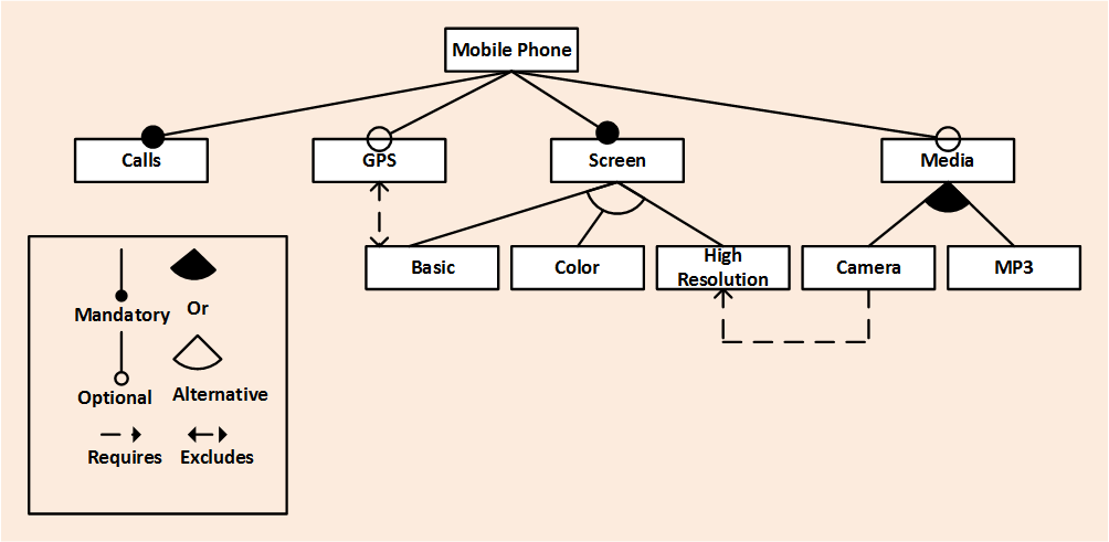
Figure 7: Feature model for mobile phone product line. To form a mobile phone, “Calls” and “Screen” are the mandatory features(shown as solid $\bullet$), while the “GPS” and “Media” features are optimal(shown as hollow $\circ$). The “Screen” feature can be “Basic“, “Color” or “High resolution” (the alternative relationship). The “Media” feature contains “camera”, “MP3”, or both (the Or relationship).

$$\left\{\begin{array}[]{ll}\neg\text{Mobile Phone}\lor\text{Calls}\\ \text{Mobile Phone}\lor\neg\text{Calls}\\ \neg\text{Mobile Phone}\lor\text{Screen}\\ \text{Mobile Phone}\lor\neg\text{Screen}\\ \text{Mobile Phone}\lor\neg\text{GPS}\\ \text{Mobile Phone}\lor\neg\text{Media}\\ \text{Media}\lor\neg\text{Camera}\\ \text{Media}\lor\neg\text{MP3}\\ \neg\text{Media}\lor\text{Camera}\lor\text{MP3}\\ \text{Screen}\lor\neg\text{Basic}\\ \text{Screen}\lor\neg\text{Color}\\ \text{Screen}\lor\neg\text{High resolution}\\ \neg\text{Screen}\lor\text{Basic}\lor\text{Color}\lor\text{High resolution}\\ \neg\text{Basic}\lor\neg\text{Color}\lor\neg\text{High resolution}\\ \text{Basic}\lor\neg\text{Color}\lor\neg\text{High resolution}\\ \neg\text{Basic}\lor\text{Color}\lor\neg\text{High resolution}\\ \neg\text{Basic}\lor\neg\text{Color}\lor\text{High resolution}\\ \neg\text{GPS}\lor\neg\text{Basic}\\ \neg\text{Camera}\lor\text{High resolution}\end{array}\right.$$

Figure 8: Figure 7 expressed as CNF

4.1.3 Software Product Lines

A software product line (SPL) is a collection of related software products, which share some core functionality [28]. From one product line, many products can be generated. For example, Apel et al. [63] model the compilation configuration parameters of databases as a product line. By adjusting those configurations, a suite of different database solutions can be generated.

Figure 7 shows a feature model for a mobile phone product line. All features are organized as a tree. The relationship between two features might be “mandatory”, “optional”, “alternative”, or “or”. Also, there exist some cross-tree constraints, which means the preferred features are not in the same sub-tree. These cross-tree constraints complicate the process of exploring feature models. In practice, all constraints, including the tree-structure constraints and the cross-tree constraints can be expressed by the CNF (conjunctive normal form). For example, Figure 7 can be expressed as the set of CNF formulas shown in Figure 8.

Researchers who explore these kinds of models [59, 58, 28, 30] define a “good” product as the one that satisfies five objectives:

1. Find the valid products (products not violating any cross-tree constraint or tree structure) which have.

2. More features; and

3. Less known defects; and

4. Less total cost; and

5. Most features used in prior applications.

Following the approach of Sayyad [58], defect, cost, and knowledge of usage in prior applications is set stochastically.

A major problem with analyzing software product lines is that it can be very hard to find valid product since real-world software product lines can be far more complex than our example. Some software product line models comprise up to tens of thousands of features, with 100,000s of constraints (see Table  I). These networks of constraints can get so complex that random assignments of “use” or “do not use” to the features have a very low probability of satisfying the constraints. For example, in one of our software product lines, the linux model, we generated 10,000 random sets of decisions for the features. Within that space, less than four decisions were valid.

Consequently, much of the research on optimizing the generation of products from a software product lines have focused on how best to optimize within these heavily-constrained models:

• Sayyad et al. [58] introduced the IBEASEED method– a five-goal optimization problem had its first generation of candidates initialized by a pre-processor that just sought out valid products (and one other goal).

• SATIBEA was introduced by Henard et al. [30]. This makes full use of SAT solver technology to fix the invalid candidates every time the “mutate” or “crossover” operation is performed in the IBEA algorithm. Results showed that the SATIBEA algorithm could find the valid products for the extremely large feature models by tens of thousands evaluations, much better than other algorithms.

To the best of our knowledge, the SATIBEA method is the best algorithm to find the optimal SPL which are represented in the form of CNFs. Consequently, we will compare Sway with SATIBEA algorithm.

We used five product line models from SPLOT and LAVT repositories. Table  I shows the basic information of our five cases. According to the number of features or constraints, the size of decision spaces of five cases are subjected to

$$\text{webportal}<\text{eshop}<\text{fiasco}\approx\text{freebsd}<\text{linux}$$ (6)

Table I: Feature models used in this study, sorted by the number of constraints. The constraints include the tree-structure and cross-tree constraints. SPLOT models can be found at http://www.splot-research.org/ and LVAT models are at https://code.google.com/archive/p/linux-variability-analysis-tools/

Name(Source)	Number of features	Number of constraints	Reference
webportal (SPLOT)	49	81	[40]
eshop (SPLOT)	330	506	[38]
fiasco (LVAT)	1638	5,228	[5]
freebsd (LVAT)	1396	62,138	[61]
linux (LVAT)	6888	343,944	[61]

Table II: Parameters tuned by grid search for the NSGA-II algorithm in solving XOMO and POM3 cases.

Name	MU	CXPB	MUTPB
OSP	200	0.9	0.1
OSP2	100	0.8	0.2
GROUND	200	0.8	0.15
FLIGHT	300	0.9	0.15
POM3a	300	0.8	0.15
POM3b	160	0.9	0.1
POM3c	200	0.9	0.2

4.2 Research Questions

To explore Sway, we organized our exploration around the following research questions (RQ):

1. (RQ1) To what extent is Sway faster than typical MOEAs?

2. (RQ2) Can Sway find the solution with maximized (minimized) objective as other MOEAs?

RQ1 questions how fast Sway is while RQ2 questions whether the results from Sway are comparable to other MOEA algorithms. Equation (3), (4) and (6) indicates the order of problem size. In the following, all results will be presented in that size order.

Table III: Parameter configurations overview

Strategy	Algorithm	Pop Size	Crossover Rate	Mutation Rate	Repeat	Termination
MOEA	NSGA-II	See Table II			30	Not improved in 5 gens
	SATIBEA	300$\dagger$	0.05	0.001*	30	Not improved in 5 gens
Sample	SWAY	10,000	/	/	30	See Algorithm 1
Brute-Force	Groud-Truth	10,000	/	/	30	Generation 0

$\dagger$ archive size = pop size = 300

* Standard mutate: 0.001; Smart mutate: 0.98

POM3 and XOMO models are optimized by NSGA-II, SWAY and GroundTruth

SPL models are optimized by SATIBEA, SWAY and GroundTruth

There are many MOEA algorithms or modified MOEA to solve our benchmarks. In the following, we compare Sway against some arguably state-of-the-art methods. Our reading of the literature is that:

• Best prior results for XOMO and POM3 were reported using NSGA-II [17, 35];

• Best prior results for configuring products from product lines were obtained using SATIBEA [30].

When applying SATIBEA to the software product line models, we used the control parameters suggested by Henard et al. [30]. As to applying NSGA-II to XOMO or POM3, prior reports [35] and [39] did not state their control parameters. To adddress that issue:

• We ran a grid search [6] for the three parameters: population size (MU), cross-over probability (CXPB) and mutation probability (MUTPB).

• Our grid search space was defined as $\{\text{MU}=[100,120,\ldots,300]\}\times\{\text{CXPB}=[0.9,0.8,\ldots,0.6]\}\times\{\text{MUTPB}=[0.1,0.15,\ldots,0.25]\}$.

• We use hypervolume (see §4.3) as the quality indicator when grid searching. Here we used hypervolume since it is the combination of convergence and diversity indicator.

• Table  II shows the tuned parameters.

Parameter tuning is necessary for SE exploration, especially in the area of search-based SE. For example, in a very recent FSE’17 paper, Fu et al. [25] found that naive learner, e.g., SVM, with parameter tuning can even outperform complex deep learning techniques.

However, when discussing this work with other researchers and colleagues, one common question is “why grid search?”. Our answer is that: “grid search” is simple enough. Even though researchers created many parameter tuners, for example, Fu [25] applied differential evolutionary optimizer, Arcuri [2] applied the central composite design to reduce the number of explored configurations, etc., grid search can cover most of the possible configurations.

In the following, whenever we mention NSGA-II, this will be that algorithm plus the parameters of Table  II.

All of our experiments were implemented using the DEAP [24] MOEA Python framework. In SATIBEA and the candidate initialization of SPL candidates, an SAT solver is required. Henard et.al [30] used the SAT4j solver. In this paper, we used PicoSAT [1] instead. We used PicoSAT since it recently achieved impressive comparative performance results in an international SAT-Race 2015 competition [4].

The termination of Sway is controlled by the minimum cluster size (see §3.3). The termination of NSGA-II and SATIBEA can be defined as maximum running time, a number of evolution generations or even manual termination, etc. In this paper, to enable a fair comparison with the state-of-the-art algorithm, we set the termination of existing MOEA algorithm as the point where solution quality does improve for consecutive five generations. Here, quality was measured by combing convergence and diversity using the hypervolume metric (see §4.3).

Finally, since there is no mutation or cross-over operations in Sway , all results are from initial random-generated candidate sets. To address the tradeoff of Sway , we also used the NSGA-II selection operator to find the Pareto frontier among the set of initial candidates. This calculation was time-consuming since it needs to evaluate all candidates (10,000 in our experiments) and sorted them. In the following, we call this method the GroundTruth. Table III concludes all parameters.

4.3 Performance Measures

Our research questions concern how fast the Sway runs and how good the results are. To explore how fast of Sway (efficiency), we record following two measures.

1. (M1) Runtime: The execution time from one algorithm starts to the terminal of that algorithm. Running time is a direct method to compare different method.

2. (M2) Number of evaluations: Sometimes comparing the running time is not enough. While all of our methods were coded in the same language (Python), some of the implementation is more mature (and have been optimized better) than others. Since, part of runtimes, we also record the number of evaluations.

To measure how good the result of Sway are (effectiveness), we followed the guidance of a recent ICSE’16 [69] paper. That guide advises to record four quality measures: generational distance, generated spread, pareto front size and hypervolume. Here we first define $PF_{c}$ and $PF_{0}$. $PF_{c}$ is the Pareto front obtained by an algorithm while $PF_{0}$ is the optimal Pareto Front for a specific problem. In SE models, it is unfeasible to obtain the optimal Pareto Front  [19]. Hence, we collected all solutions found by any algorithm and picked up all non-dominated solutions to form the $PF_{0}$. This strategy is widely applied in the area of MOEA applications [69].  

1. (M3) Generational Distance (GD): GD is a measure for convergence. It is the Euclidean distance between solutions in $PF_{c}$ and nearest solutions in $PF_{0}$ [66]. It can be calculated by

   $$GD=\frac{\sqrt{\sum^{|PF_{c}|}_{i=1}d(x_{i},PF_{0})^{2}}}{|PF_{c}|}$$ (7)

   where $d(x_{i},PF_{0})$ refers to the minimum Euclidean distance from solution $x_{i}$ in $PF_{c}$ to $PF_{0}$. A lower GD indicates the result is closer to the Pareto frontier of a specific problem. A value of 0 means that all obtained solutions are optimal; i.e. lower values of GD are better.

2. (M4) Generated Spread (GS): GS [75] is a diversity indicator. It is defined to extend the quality indicator Spread which only works for bi-objective problems. GS can be calculated by

   $$GS=\frac{\sum^{m}_{i=1}d(e_{i},PF_{c})+\sum_{x\in PF_{c}}|d(x,PF_{c})-\bar{d}|}{\sum^{m}_{i=1}d(e_{i},PF_{c})+|PF_{c}|*\bar{d}}$$ (8)

   where $(e_{1},e_{2},\ldots,e_{m})$ refers to $m$ extreme solutions for each objective in $PF_{0}$; $d(*,\dagger)$ refers to the minimum Euclidean distance from solution $*$ to the set $\dagger$; $\bar{d}$ is the mean value of $d(x,PF_{c})$ for all solutions in $PF_{c}$. A lower value of GS shows that the results have a better distribution; i.e. lower values of GS are better.

   

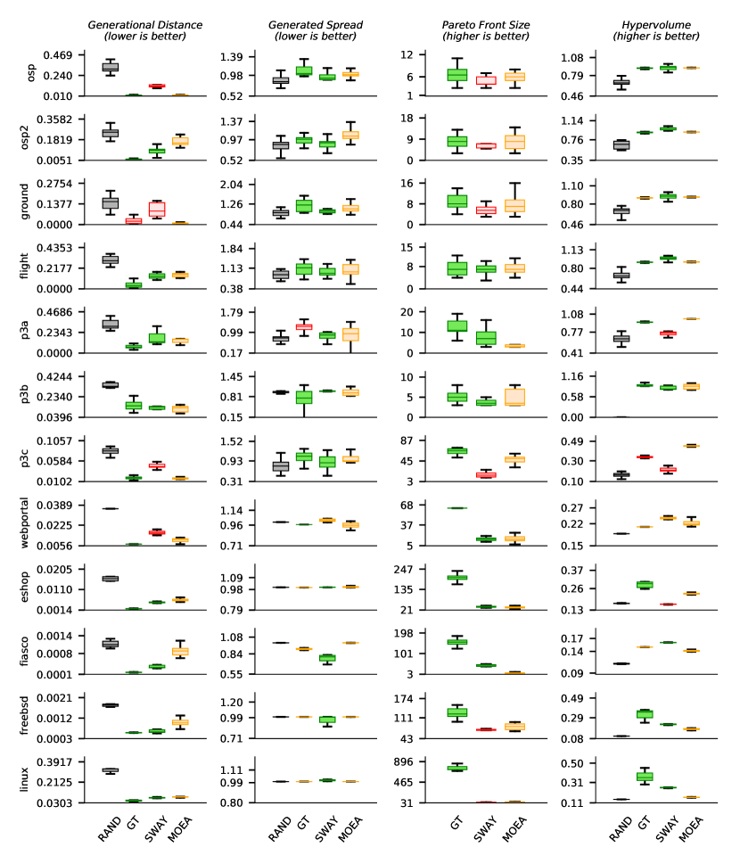
   Figure 9: The box-plot of four quality indicators in each study cases (30 runs). In a boxplot, the middle “box” represents the middle 50% of results among all 30 runs and the line dividing “box” into two parts shows the median of all runs. The upper/lower “whiskers” mark the extreme results outside middle 50% of all runs. In each plot: RAND=“sanity check” – randomly generated candidates (size = MOEA’s pareto front size); GT= GroundTrue (the frontier of 10k random generated populations); Sway = the method proposed in this paper; MOEA=the prior state-of-the-art MOEA for that corresponding study case. Recall that “generational distance” is a coverage indicator; “generated spread” and “Pareto front size” are diversity indicators; and “hypervolume” is a combination of convergence and diversity. Note that higher values are better for “Pareto front size” and “hypervolume” while lower values are better for “generational distance” and “generated spread”. Using a Wilcoxon test (5% significance level) we color these results as follows: ORANGE boxes mark results that are statistically insignificantly different from state-of-the-art method; and GREEN, RED marks results that are statistically significant better, worse (respectively) than the state-of-the-art. For a summary of these results, see Figure 10 and Figure 11.

3. (M5) Pareto front size (PFS): PFS is another diversity indicator. It measures the number of solutions included in $PF_{c}$, i.e. $|PF_{c}|$. A higher PFS means that the users have more options to choose, that is, a more diverse obtained Parto front; i.e. higher values of PFS are better.

4. (M6) Hypervolume (HV): HV is the combination of convergence and diversity indicator. As defined in [77], HV measures the size of space the obtained frontier covered. Formally,

   $$\text{Hypervolume}=\lambda\left(\bigcup_{x\in PF_{c}}\{x^{\prime}|x\prec x^{\prime}\prec x_{\text{ref}}\}\right)$$ (9)

   where $\lambda(\cdot)$ is the Lebesgue measure, the standard way measures the subset of n-dimensional Euclidean space. For example, the Lebesgue measure is the length, area or volume when the number of dimensions is $n=1,2,3$ respectively; $\prec$ is the binary domination comparator; $x_{\text{ref}}$ denotes a reference point which should be dominated by all obtained solutions. Note that, in this study, all objectives are normalized to $[0,1]$ and set $x_{\text{ref}}=(1,1,\ldots,1)$. Notice that a higher value of HV demonstrates a better performance of $PF_{c}$; higher values of Hypervolume are better.

To test the performance robustness and reduce the observational error, we repeated these case studies 30 times with 30 different random seeds. To simulate real practice, such random seeds are used in initial population creation as well as the successive process. To check the statistical significance of the differences between the algorithms, we performed a statistical test using Wilcoxon test at a 5% significance level. Wilcoxon test is a non-parametric test and suitable for the samples when the population cannot be assumed to be normally distributed.

Table IV: Median value of runtime and model evaluation numbers from 30 independent runs. Numbers rounded to the nearest percent (so “0%” means “less than 0.005”)

	Runtime(seconds)			# Evaluations
	Sway ($R_{S}$)	MOEA ($R_{M}$)	$\frac{R_{S}}{R_{S}+R_{M}}$	Sway ($E_{S}$)	MOEA ($E_{M}$)	$\frac{E_{S}}{E_{S}+E_{M}}$
osp	3.23	320	1%	18	4630	0%
osp2	3.31	112	3%	16	2432	1%
ground	3.29	388	1%	20	5321	0%
flight	5.62	663	1%	33	10980	1%
POM3a	4.69	450	1%	26	3836	1%
POM3b	5.01	583	1%	32	4532	1%
POM3b	6.33	990	1%	40	8302	0%
webportal	6	244	2%	134	5100	3%
eshop	18	321	5%	136	6732	2%
fiasco	63	1065	6%	122	20102	1%
freebsd	188	2058	8%	136	26146	1%
linux	1103	3295	25%	168	8900	2%

		Generational	Generated	Pareto	Hyper-
n	model	Distance	Spread	Front Size	volume
1	osp	0.5	1.95	0.46	0.6
2	ops2	1.30	0.82	0.72	0.65
3	ground	0.79	0.86	0.71	0.30
4	flight	1.96	0.86	0.42	0.52
5	pom3a	0.79	0.53	01.30	0.85
6	pom3b	0.75	0.43	0.56	0.85
7	pom3c	0.69	0.42	0.82	1.03
8	webportal	0.63	0.90	1.86	0.63
9	eshop	0.74	0.29	1.23	1.29
10	fiasco	1.97	0.49	1.99	0.23
11	freebsd	0.79	0.22	1.98	0.63
12	linux	0.72	0.13	1.99	1.97
	same + better	11/12	11/12	12/12	11/12

Figure 10: GroundTruth vs state-of-the-art: How often is ground truth worse, same, or better? Summarized from Figure 9. Color patterns are the same as Figure 9. Decimal in each cell is the effect size. Generating and evaluating all the models in this figure took 52 hours of CPU.

		Generational	Generated	Pareto	Hyper-
n	model	Distance	Spread	Front Size	volume
1	osp	1.97	0.45	0.36	0.63
2	ops2	0.99	0.56	0.46	0.49
3	ground	0.93	0.60	0.46	0.64
4	flight	0.72	0.63	0.49	0.59
5	pom3a	0.67	0.50	1.93	1.58
6	pom3b	0.67	0.84	0.69	0.66
7	pom3c	1.57	0.54	1.44	1.41
8	webportal	1.97	0.63	0.69	1.00
9	eshop	0.78	0.67	0.49	1.56
10	fiasco	1.23	1.63	0.96	0.99
11	freebsd	0.78	0.64	0.88	1.53
12	linux	1.04	0.69	0.63	1.92
	same + better	8/12	11/12	6/12	8/12

Figure 11: Sway vs state-of-the-art: How often is Sway worse, same, or better? Summarized from Figure 9.Color patterns are the same as Figure 9. Decimal in each cell is the effect size. Generating and evaluating all the models in this figure took the runtimes seen in Table IV.

5 Results

5.1 RQ1: is Sway Faster than Typical MOEAs?

We compared the speed of the algorithms through their runtime as well as the number of model evaluations. Table  IV shows the median runtime and evaluation numbers recorded in our experiments. As can be seen in all cases, Sway is faster than the state-of-the-art evaluation algorithms, often by two orders of magnitude (especially for the smaller models at the top of the table). And even for the largest models, Sway offered some speed up advantages. For example, in the study case linux, the median runtime of Sway was 1103s (18min), while the runtime of SATIBEA algorithm was near an hour.

Consequently, from Table  IV, our answer to RQ1 is Sway usually terminates orders of magnitude faster of the other algorithms used in this evaluation.

5.2 RQ2: Are Sway ’s Solutions as good as Other Optimizers?

Figure 9 shows boxplot of quality indicators among the 30 independent runs in our experiment (where each run used a different random number seed). In that figure:

• The RAND method is a “sanity check” for our technology. In this approach, $N$ candidates were generated at random and then pruned to a final frontier by discarding any dominated points (domination computed from §2.3). Note that, to select $N$ for this method, we used the strategy of [52]: i.e., set $N$ to the median size of the frontier generated by was used by MOEA.

• The GroundTruth method, introduced in §4.2, generates and evaluates many solutions, then reports the best parts of the Pareto frontier (found using the NSGA-II sorting strategy).

• The Sway method randomly generates solutions, and then fetch some of them through the sampling strategies described in §3. Note that Sway only evaluates a very small number of solutions.

• The MOEA method refers to the state-of-the-art method defined for each case study. Recall from §4.1 that this state-of-the-art is one of (a) the grid-search-tuned NSGA-II or (b) combining the SAT solver and IBEA algorithm.

In Figure 9, the colors denote a statistical comparison with the state of the art, where the statistical test is a non-parametric Wilcoxon comparisons at a 5% significance level:

• GREEN, RED denote results at are better, worse (respectively) than the state-of-the-art;

• Results that statistically insiginficantly different to the state-of-the-art are marked in ORANGE.

Figure 10 and Figure 11 summarize Figure 9 using the same color scheme. As shown in Figure 10, GroundTruth often found best results. At first glance, the results of Figure 10 seem to say that all work on heuristic multi-objective optimization should halt since merely making up lots of random solutions performs comparatively very well indeed. However, not shown in Figure 10 is the CPU time to achieve those results. Recall from Table IV that Sway required just under 25 minutes to optimize all the models of this paper (and 80% of that time was spent on the largest linux model). By way of comparison, evaluating all the solutions in Figure 10 required 52 hours; i.e., that approach was 124 times slower. Figure 11 comments on the value of the solutions achieved via that very slow random GroundTruth method vs Sway.

Figure 11 summarizes the results achieved by Sway. In the majority case, across all performance measures, Sway performs the same or better as the state-of-the-art. Note that these results were achieved with the number of evaluations seem in Table  IV; i.e. after merely dozens to a few hundred evaluations.

One quirk in Figure 9 is that sometimes, very simple RAND method achieved comparable generated spread values to MOEA or Sway . This is due to the nature of solutions in multi-dimensional space. As noted by Domingos, random points in large dimensions space are often very distant [20]. Hence, it is not surprising that a random selection does very well (as measured by spread). Note that achieving good spread scores via random methods says nothing about the value of the optimizations achieved via that method (merely the dispersion of those candidates). For a comment on the value of the optimization achieved, see the generational distance and hypervolume results of Figure 9 where, as we would expect, RAND performs much worse than other optimizers.

6 Threats to Validity

6.1 Optimizer bias

The goal of this paper was not to prove that Sway is the best optimizer for all models. Rather, our goal was to say that, compared to current practice in the literature, Sway offers competitive solutions at a small fraction of the evaluation costs of other methods. Hence, we propose Sway as a reasonable first choice for benchmarking other approaches.

For that goal, it is not necessary to compare Sway against all other optimizers. Rather, Sway should be compared against known state-of-the-art in the literature.

6.2 Internal bias

Internal bias originates from the stochastic nature of multi-objective optimization algorithms. The evolutionary process required many random operations, same as the Sway introduced in this paper.

To mitigate these threats, we repeated our experiments for 30 runs and reported the median/boxplot of the indicators. We also employed statical tests to check the significance of the achieved results.

6.3 Sampling bias

This paper studied the performance of Sway using three classes of models: XOMO, POM3, and software product lines. There are many other optimization problems in the area of software engineering, and it is possible that the results of this paper will not apply to those models. Future research should explore more models to check the validity of our results.

7 Related Work

We introduced a baseline method to solve the SBSE problems through sampling. Many researchers tried to solve the tricky or computationally expensive problems through sampling and other strategies in other domains.

For example, sampling has been successively applied to the noisy real-word optimization problems by Cantu-Paz [11]. They introduced an adaptive sampling policy which they test on a 100-bit onemax function. While Cantu-Paz demonstrated that the adaptive sampling could find better solutions, from our perspective, the drawback with that work is that it requires far more computation time.

Shahrzad et al. [60] analyzed the advantage of age-layering in an evolutionary algorithm as well. In aged-layered evolutionary algorithms, a small sample of candidates are evaluated first; and if they seem promising, they are evaluated with more samples. The age-layering method effectively reduces the fitness evaluations and speedups the evolution process. However, at least for the aged-layered algorithm reported by Shahrzad et al. [60], this approach still requires millions of model evaluations, Hence, it would not be a candidate for a baseline SBSE method.

(1+1) EA is another strategy which can reduce the computing intensity of evolution algorithms [21]. In (1+1) EA, the population size is set to one. The candidate is mutated in some probability and then replaces the former one if better fitness is found. Compared to the common evolution algorithms which population size can up to hundreds or even thousands, the (1+1) EA can significantly reduce the fitness evaluations [21]. But the drawback for standard (1+1) EA is that it did not naturally handle models with multi-objectives, or conflicting objectives, which are very common in SBSE.

Another strategy to speed up the evolutionary algorithms is the use of a surrogate model. Ong et al. [51] presented a parallel evolutionary algorithm which leverages surrogate model for solving the computational expensive design problems. A surrogate model is a statical model built to approximate the computationally expensive model. They created a surrogate model basing on the radial basis function. The computation of RBF is much cheaper than the original model. But the precise of surrogate model strongly depends on the evaluated candidates. To improve the precision of surrogate model for search-based software engineering problems, we have to enlarge the number of model evaluations [60].

8 Conclusions and Future Work

Wolpert et al. [72] caution no optimization algorithm always works best for all domains. Hence, when encountering a new domain, multiple methods should be applied.

When applying multiple methods, it is useful to have a very fast baseline method to try first since:

• That offers a useful baseline which can be used to understand the relative value of other methods.

• If this initial baseline method achieved adequate results, the search through the other methods can stop sooner.

For these reasons, many researchers in the field of SE [71, 48, 62, 33] and elsewhere [16, 32] note that any field that conducts empirical experiments with algorithms can utilize baseline methods. Such baselines allow for early feedback about whether or not the optimization is correctly integrated into the model. They can also be used as scouts that run ahead of more expensive processes to report the complexity of up-coming tasks. For example, Shepperd and Macdonnel [62] argue convincingly that measurements are best viewed as ratios compared to measurements taken from some minimal baseline method.

In this paper, we introduced a baseline method, Sway, to explore optimization problems in the context of search-based software engineering problems. Sway can find promising individuals among a large set of candidates using a very small number of model evaluations. Since the number of required model evaluations is much less than that of common evolutionary algorithms, Sway terminates very early. Sway would be especially useful when the model evaluation is computation expensive (i.e., very slow).

Sway satisfies all the criteria of a baseline method, introduced in §2.1; e.g., simple to code, applicable to a wide range of models. This paper tested Sway via numerous scenarios within three SE models. These models differed in their type of decisions as well as the size of their decision space. Results showed the quality of outputs from Sway were comparable to the state-of-the-art evolutionary algorithms for those specific problems. Sway is also very fast. Among 15 cases studied in this paper, Sway only requires less than 5% (in median) of the runtime of the standard evolutionary algorithms, but in majority case across all performance measures, Sway performs the same or better as the state-of-the-art.

Extending this work in several ways is possible. In this paper, we have explored three SE models from the areas of effort estimation, project management as well as requirement engineering. There are many other domains in SE that might benefit from this approach such as testing, debugging and cloud environment configuration, etc. For example, Wang et al. [67] introduced a regression test selection for service-oriented workflow applications. We also have further research in configuring the workflows into cloud environment basing on Sway  [12]. In our future work, we will explore the sampling techniques in service-oriented workflow applications as well as other SE models.

Second, we introduced the Sway for two types of decision space – continuous decision spaces (§3.1) and binary decision spaces (§3.2). In the future, we will explore more types of problems, for example, the graph-based models like software modularization [29].

Third, the parameters of Sway , such as “enough” in Algorithm 2, were set manually in this paper. Discussion of relations between these parameters and final results is left for future work.

Finally, in Figure 9 we can find that the GroundTruth method is almost always comparable to the MOEA methods. But the Sway is beat by the MOEA in some cases. This is the tradeoff of Sway ’s fast termination. Can we increase the number of model evaluation in some strategy to improve the quality? This is worth exploring.

Jianfeng Chen is a computer science PhD candidate at North Carolina State University. He received his bachelor degree in Shandong University, China. His research relates to automated software engineering, artificial intelligence and multi-objectives optimization (with a particular focus on utilizing stochastic sampling techniques to speed up search-based software engineering solvers). He also explores methods relating to fuzz testing, regression testing and cloud environment configurations. He has published papers in IEEE Transactions on Software Engineering, Information Software Technology, International Symposium on Search Based Software Engineering. For more, see his homepage http://jianfeng.us.

Vivek Nair is a fifth year Ph.D. student in department of Computer Science at North Carolina State University. He received his bachelor and master degree in West Bengal University of Technology and National Institute of Technology, Durgapur respectively. His primary interest lies in the exploring possibilities of using multi-objective optimization to solve problems in Software Engineering. He is currently working on performance prediction models of highly configurable systems. He received his master degree and worked in the mobile industry for a period of 2 years before returning to graduate school. For more information, visit http://vivekaxl.com.

Rahul Krishna is a third year Ph.D. student in the department of Computer Science at North Carolina State University. He received his master’s degree in Electrical Engineering also at North Carolina State University. His primary interest lies in exploring ways in which aspects of pattern recognition and artificial intelligence can be used to generate actionable analytics for software engineering. He currently works on developing machine learning algorithms that go beyond prediction to generate insights to assist decision making. He also works on transfer learning methodologies that can help transfer models between software projects. For more information, visit http://rkrsn.us.

Tim Menzies (Ph.D., UNSW, 1995) is a full Professor in CS at North Carolina State University, where he explores SE, data mining, AI, search-based SE, and open access science. He is the author of over 250 referred publications and co-founder of the PROMISE conference series devoted to reproducible experiments in SE (http://tiny.cc/seacraft). Dr. Menzies also serves as associated editor of many journals: IEEE Transactions on Software Engineering (2010 to 2016), ACM Transactions on Software Engineering Methodologies, Empirical Software Engineering, the Automated Software Engineering Journal the Big Data Journal, Information Software Technology, IEEE Software, and the Software Quality Journal. He has served as co-general chair of ICSME’16 and co-PC chair for ASE’12, ICSE’15, SSBSE’17. For more, see http://menzies.us.

References

- [1] Boolector at the SMT competition 2016. Technical report, FMV Reports Series, Institute for Formal Models and Verification, Johannes Kepler University, Altenbergerstr. 69, 4040 Linz, Austria, 2016.
- [2] Andrea Arcuri and Gordon Fraser. Parameter tuning or default values? an empirical investigation in search-based software engineering. Empirical Software Engineering, 18(3):594–623, 2013.
- [3] Danilo Ardagna, Giovanni Paolo Gibilisco, Michele Ciavotta, and Alexander Lavrentev. A multi-model optimization framework for the model driven design of cloud applications. In International Symposium on Search Based Software Engineering, pages 61–76. Springer, 2014.
- [4] Tomáš Balyo, Armin Biere, Markus Iser, and Carsten Sinz. Sat race 2015. Artificial Intelligence, 241:45–65, 2016.
- [5] Thorsten Berger, Steven She, Rafael Lotufo, Andrzej Wasowski, and Krzysztof Czarnecki. Variability modeling in the systems software domain. Generative Software Development Laboratory, University of Waterloo, Technical Report, 2012.
- [6] James Bergstra and Yoshua Bengio. Random search for hyper-parameter optimization. Journal of Machine Learning Research, 13(Feb):281–305, 2012.
- [7] Leonora Bianchi, Marco Dorigo, Luca Maria Gambardella, and Walter J. Gutjahr. A survey on metaheuristics for stochastic combinatorial optimization. Natural Computing, 8(2):239–287, 2009.
- [8] B. Boehm and R. Turner. Using risk to balance agile and plan-driven methods. Computer, 36(6):57–66, 2003.
- [9] Barry Boehm, Ellis Horowitz, Ray Madachy, Donald Reifer, Bradford K. Clark, Bert Steece, A. Winsor Brown, Sunita Chulani, and Chris Abts. Software Cost Estimation with Cocomo II. Prentice Hall, 2000.
- [10] Barry Boehm and Richard Turner. Balancing Agility and Discipline: A Guide for the Perplexed. Addison-Wesley Longman Publishing Co., Inc., 2003.
- [11] Erick Cantú-Paz. Adaptive sampling for noisy problems. In Genetic and Evolutionary Computation Conference, pages 947–958. Springer, 2004.
- [12] Jianfeng Chen and Tim Menzies. Riot: a novel stochastic method for rapidly configuring cloud-based workflows. arXiv preprint arXiv:1708.08127, 2017.
- [13] Jianfeng Chen, Vivek Nair, and Tim Menzies. Beyond evolutionary algorithms for search-based software engineering. Information and Software Technology, pages –, 2017.
- [14] Kai-Min Chung, Wei-Chun Kao, Chia-Liang Sun, Li-Lun Wang, and Chih-Jen Lin. Radius margin bounds for support vector machines with the rbf kernel. Neural computation, 15(11):2643–2681, 2003.
- [15] Vincent A Cicirello and Stephen F Smith. Modeling genetic algorithm performance for control parameter optimization. In Proceedings of the 2nd Annual Conference on Genetic and Evolutionary Computation, pages 235–242. Morgan Kaufmann Publishers Inc., 2000.
- [16] P R Cohen. Empirical Methods for Artificial Intelligence. MIT Press, 1995.
- [17] Kalyanmoy Deb, Samir Agrawal, Amrit Pratap, and Tanaka Meyarivan. A fast elitist non-dominated sorting genetic algorithm for multi-objective optimization: Nsga-ii. In International Conference on Parallel Problem Solving From Nature, pages 849–858. Springer, 2000.
- [18] Kalyanmoy Deb, Amrit Pratap, Sameer Agarwal, and TAMT Meyarivan. A fast and elitist multiobjective genetic algorithm: Nsga-ii. IEEE transactions on evolutionary computation, 6(2):182–197, 2002.
- [19] Kalyanmoy Deb, Lothar Thiele, Marco Laumanns, and Eckart Zitzler. Scalable Test Problems for Evolutionary Multi-Objective Optimization. TIK Report 1990, Computer Engineering and Networks Laboratory (TIK), ETH Zurich, July 2001.
- [20] Pedro Domingos. A few useful things to know about machine learning. Communications of the ACM, 55(10):78–87, 2012.
- [21] Stefan Droste, Thomas Jansen, and Ingo Wegener. On the analysis of the (1+ 1) evolutionary algorithm. Theoretical Computer Science, 276(1-2):51–81, 2002.
- [22] Christos Faloutsos and King-Ip Lin. Fastmap: a fast algorithm for indexing, data-mining and visualization of traditional and multimedia datasets. In ACM SIGMOD international conference on Management of data, 1995.
- [23] Filomena Ferrucci, Mark Harman, Jian Ren, and Federica Sarro. Not going to take this anymore: multi-objective overtime planning for software engineering projects. In Proceedings of the 2013 International Conference on Software Engineering, pages 462–471. IEEE Press, 2013.
- [24] Félix-Antoine Fortin, François-Michel De Rainville, Marc-André Gardner, Marc Parizeau, and Christian Gagné. DEAP: Evolutionary algorithms made easy. Journal of Machine Learning Research, 13:2171–2175, jul 2012.
- [25] Wei Fu and Tim Menzies. Easy over hard: A case study on deep learning. arXiv preprint arXiv:1703.00133, 2017.
- [26] Wei Fu, Tim Menzies, and Xipeng Shen. Tuning for software analytics: Is it really necessary? Information and Software Technology, 76:135–146, 2016.
- [27] Mark Harman, Syed Islam, Yue Jia, Leandro L Minku, Federica Sarro, and Komsan Srivisut. Less is more: Temporal fault predictive performance over multiple Hadoop releases. In International Symposium on Search Based Software Engineering, pages 240–246. Springer, 2014.
- [28] Mark Harman, Yue Jia, Jens Krinke, William B Langdon, Justyna Petke, and Yuanyuan Zhang. Search based software engineering for software product line engineering: a survey and directions for future work. In Proceedings of the 18th International Software Product Line Conference-Volume 1, pages 5–18. ACM, 2014.
- [29] Mark Harman, Stephen Swift, and Kiarash Mahdavi. An empirical study of the robustness of two module clustering fitness functions. In Proceedings of the 7th annual conference on Genetic and evolutionary computation, pages 1029–1036. ACM, 2005.
- [30] Christopher Henard, Mike Papadakis, Mark Harman, and Yves Le Traon. Combining multi-objective search and constraint solving for configuring large software product lines. In Software Engineering (ICSE), 2015 IEEE/ACM 37th IEEE International Conference on, volume 1, pages 517–528. IEEE, 2015.
- [31] John H. Holland. Genetic Algorithms. Scientific American, 267(1):66–72, 1992.
- [32] R C Holte. Very Simple Classification Rules Perform Well on Most Commonly Used Datasets. Machine Learning, 11:63, 1993.
- [33] B a Kitchenham, E Mendes, and G H Travassos. Cross- vs. Within-Company Cost Estimation Studies: A Systematic Review. IEEE Transactions on Software Engineering, 33(5):316–329, 2007.
- [34] Sven Kosub. A note on the triangle inequality for the Jaccard distance. arXiv preprint arXiv:1612.02696, 2016.
- [35] J. Krall, T. Menzies, and M. Davies. Gale: Geometric active learning for search-based software engineering. IEEE Transactions on Software Engineering, 41(10):1001–1018, Oct 2015.
- [36] J. Krall, T. Menzies, and M. Davies. Learning mitigations for pilot issues when landing aircraft (via multiobjective optimization and multiagent simulations). IEEE Transactions on Human-Machine Systems, 46(2):221–230, April 2016.
- [37] Joseph Krall, Tim Menzies, and Misty Davies. Learning the task management space of an aircraft approach model. In Proceedings of the 2014 AAAI Conference, AAAI’14, 2014.
- [38] Sean Quan Lau. Domain analysis of e-commerce systems using feature-based model templates. University of Waterloo Ontario, Canada, 2006.
- [39] Naveen Kumar Lekkalapudi. Cross trees: Visualizing estimations using decision trees. WEST VIRGINIA UNIVERSITY, 2014.
- [40] Marcílio Mendonça, Thiago Tonelli Bartolomei, and Donald Cowan. Decision-making coordination in collaborative product configuration. In Proceedings of the 2008 ACM symposium on Applied computing, pages 108–113. ACM, 2008.
- [41] Tim Menzies, Robert F. Cohen, Sam Waugh, and Simon Goss. Applications of abduction: Testing very long qualitative simulations. IEEE Transactions on Knowledge and Data Engineering, 14(6):1362–1375, 2002.
- [42] Tim Menzies and Paul Compton. Applications of abduction: Hypothesis testing of neuroendocrinological qualitative compartmental models. Artificial intelligence in medicine, 10(2):145–175, 1997.
- [43] Tim Menzies and Bojan Cukic. When to test less. IEEE Software, 17(5):107–112, 2000.
- [44] Tim Menzies, Oussama El-Rawas, J. Hihn, M. Feather, B. Boehm, and R. Madachy. The business case for automated software engineerng. In ASE ’07: Proceedings of the twenty-second IEEE/ACM international conference on Automated software engineering, pages 303–312, New York, NY, USA, 2007. ACM.
- [45] Tim Menzies and Julian Richardson. Xomo: Understanding development options for autonomy. In COCOMO forum, volume 2005, 2005.
- [46] Tim Menzies, S. Williams, Oussama El-Rawas, D. Baker, B. Boehm, J. Hihn, K. Lum, and R. Madachy. Accurate estimates without local data? Software Process Improvement and Practice, 14:213–225, July 2009.
- [47] Tim Menzies, S. Williams, Oussama El-Rawas, B. Boehm, and J. Hihn. How to avoid drastic software process change (using stochastic stability). In ICSE’09, 2009.
- [48] Nikolaos Mittas and Lefteris Angelis. Ranking and Clustering Software Cost Estimation Models through a Multiple Comparisons Algorithm. IEEE Transactions of Software Engineering, 2013.
- [49] Vivek Nair, Tim Menzies, and Jianfeng Chen. An (accidental) exploration of alternatives to evolutionary algorithms for sbse. In International Symposium on Search Based Software Engineering, pages 96–111. Springer, 2016.
- [50] Vinicius Paulo L Oliveira, Eduardo FD Souza, Claire Le Goues, and Celso G Camilo-Junior. Improved crossover operators for genetic programming for program repair. In International Symposium on Search Based Software Engineering, pages 112–127. Springer, 2016.
- [51] Yew S Ong, Prasanth B Nair, and Andrew J Keane. Evolutionary optimization of computationally expensive problems via surrogate modeling. AIAA journal, 41(4):687–696, 2003.
- [52] Ali Ouni, Raula Gaikovina Kula, Marouane Kessentini, Takashi Ishio, Daniel M German, and Katsuro Inoue. Search-based software library recommendation using multi-objective optimization. Information and Software Technology, 83:55–75, 2017.
- [53] David Owen, Bojan Cukic, and Tim Menzies. An alternative to model checking: Verification by random search of and-or graphs representing finite-state models. In High Assurance Systems Engineering, 2002. Proceedings. 7th IEEE International Symposium on, pages 119–126. IEEE, 2002.
- [54] David Owen, Tim Menzies, and Bojan Cukic. What makes finite-state models more (or less) testable? In Automated Software Engineering, 2002. Proceedings. ASE 2002. 17th IEEE International Conference on, pages 237–240. IEEE, 2002.
- [55] John C. Platt. Fastmap, metricmap, and landmark MDS are all nystrom algorithms. In In Proceedings of 10th International Workshop on Artificial Intelligence and Statistics, pages 261–268, 2005.
- [56] D. Port, A. Olkov, and T. Menzies. Using simulation to investigate requirements prioritization strategies. In Automated Software Engineering, pages 268–277, 2008.
- [57] Federica Sarro, Filomena Ferrucci, Mark Harman, Alessandra Manna, and Jian Ren. Adaptive multi-objective evolutionary algorithms for overtime planning in software projects. IEEE Transactions on Software Engineering, 2017.
- [58] A. Sayyad, J. Ingram, T. Menzies, and H. Ammar. Scalable product line configuration: A straw to break the camel’s back. In ASE’13, Palo Alto, CA, 2013.
- [59] Abdel Salam Sayyad, Tim Menzies, and Hany Ammar. On the value of user preferences in search-based software engineering: A case study in software product lines. In Proceedings of the 2013 International Conference on Software Engineering, ICSE ’13, pages 492–501, 2013.
- [60] Hormoz Shahrzad, Babak Hodjat, and Risto Miikkulainen. Estimating the advantage of age-layering in evolutionary algorithms. In Proceedings of the 2016 on Genetic and Evolutionary Computation Conference, pages 693–699. ACM, 2016.
- [61] Steven She, Rafael Lotufo, Thorsten Berger, Andrzej Wøsowski, and Krzysztof Czarnecki. Reverse engineering feature models. In Software Engineering (ICSE), 2011 33rd International Conference on, pages 461–470. IEEE, 2011.
- [62] Martin J. Shepperd and Steven G. MacDonell. Evaluating prediction systems in software project estimation. Information & Software Technology, 54(8):820–827, 2012.
- [63] Norbert Siegmund, Sergiy S Kolesnikov, Christian Kästner, Sven Apel, Don Batory, Marko Rosenmüller, and Gunter Saake. Predicting performance via automated feature-interaction detection. In Proceedings of the 34th International Conference on Software Engineering, pages 167–177. IEEE Press, 2012.
- [64] T. Menzies V. Nair and J.Chen. An (accidental) exploration of alternatives to evolutionary algorithms for sbse. In SSBSE’16, 2016.
- [65] Varsha Veerappa and Emmanuel Letier. Understanding clusters of optimal solutions in multi-objective decision problems. In Proceedings of the 2011 IEEE 19th International Requirements Engineering Conference, RE 2011, pages 89–98, 2011.
- [66] David A. Van Veldhuizen and Gary B. Lamont. Evolutionary computation and convergence to a pareto front. In Stanford University, California, pages 221–228. Morgan Kaufmann, 1998.
- [67] Hongda Wang, Jianchun Xing, Qiliang Yang, Ping Wang, Xuewei Zhang, and Deshuai Han. Optimal control based regression test selection for service-oriented workflow applications. Journal of Systems and Software, 124:274–288, 2017.
- [68] Shuai Wang, Shaukat Ali, and Arnaud Gotlieb. Minimizing test suites in software product lines using weight-based genetic algorithms. In Proceedings of the 15th annual conference on Genetic and evolutionary computation, pages 1493–1500. ACM, 2013.
- [69] Shuai Wang, Shaukat Ali, Tao Yue, Yan Li, and Marius Liaaen. A practical guide to select quality indicators for assessing pareto-based search algorithms in search-based software engineering. In Proceedings of the 38th International Conference on Software Engineering, pages 631–642. ACM, 2016.
- [70] Tiantian Wang, Mark Harman, Yue Jia, and Jens Krinke. Searching for better configurations: A rigorous approach to clone evaluation. In 9th Joint Meeting on Foundations of Software Engineering. ACM, 2013.
- [71] Peter A. Whigham, Caitlin A. Owen, and Stephen G. Macdonell. A baseline model for software effort estimation. ACM Trans. Softw. Eng. Methodol., 24(3):20:1–20:11, May 2015.
- [72] D. H. Wolpert and W. G. Macready. No free lunch theorems for optimization. Trans. Evol. Comp, 1(1):67–82, April 1997.
- [73] Shin Yoo, Mark Harman, and Shmuel Ur. Gpgpu test suite minimisation: search based software engineering performance improvement using graphics cards. Empirical Software Engineering, 18(3):550–593, 2013.
- [74] Yuanyuan Zhang, Mark Harman, and A Mansouri. The sbse repository: A repository and analysis of authors and research articles on search based software engineering. CREST Centre, UCL, crestweb.cs.ucl.ac.uk/resources/sbse _repository, 2016.
- [75] Aimin Zhou, Yaochu Jin, Qingfu Zhang, Bernhard Sendhoff, and Edward Tsang. Combining model-based and genetics-based offspring generation for multi-objective optimization using a convergence criterion. In Evolutionary Computation, 2006. CEC 2006. IEEE Congress on, pages 892–899. IEEE, 2006.
- [76] Eckart Zitzler and Simon Künzli. Indicator-based selection in multiobjective search. In International Conference on Parallel Problem Solving from Nature, pages 832–842. Springer, 2004.
- [77] Eckart Zitzler and Lothar Thiele. Multiobjective evolutionary algorithms: a comparative case study and the strength pareto approach. IEEE transactions on evolutionary computation,, 3(4):257–271, 1999.
- [78] Marcela Zuluaga, Andreas Krause, Guillaume Sergent, and Markus Püschel. Active learning for multi-objective optimization. In International Conference on Machine Learning (ICML), 2013.