Wide-Band Spectra of Giant Radio Pulses from the Crab Pulsar

Abstract

We present the results of the simultaneous observation of the giant radio pulses (GRPs) from the Crab pulsar at 0.3, 1.6, 2.2, 6.7, and 8.4 GHz with four telescopes in Japan. We obtain 3194 and 272 GRPs occurring at the main pulse and the interpulse phases, respectively. A few GRPs detected at both 0.3 and 8.4 GHz are the most wide-band samples ever reported. In the frequency range from 0.3 to 2.2 GHz, we find that about 70% or more of the GRP spectra are consistent with single power laws and the spectral indices of them are distributed from $-4$ to $-1$. We also find that a significant number of GRPs have such a hard spectral index (approximately $-1$) that the fluence at 0.3 GHz is below the detection limit (“dim-hard” GRPs). Stacking light curves of such dim-hard GRPs at 0.3 GHz, we detect consistent enhancement compared to the off-GRP light curve. Our samples show apparent correlations between the fluences and the spectral hardness, which indicates that more energetic GRPs tend to show softer spectra. Our comprehensive studies on the GRP spectra are useful materials to verify the GRP model of fast radio bursts in future observations.

1. Introduction

From several pulsars, sporadic intense radio pulses that are much brighter than the normal pulse flux, called “Giant Radio Pulses (GRPs)”, are observed. The distinctive feature of GRPs is that their amplitude distribution follows a power law (e.g. Argyle & Gower, 1972), while that of “normal” pulses follows a log-normal distribution (Burke-Spolaor et al., 2012). GRPs are detected from about 10 pulsars, including some young pulsars such as the Crab pulsar (PSR B0531+21) (e.g. Majid et al., 2011) and PSR B0540-69 (Johnston & Romani, 2003), and some millisecond pulsars such as PSR B1937+21 (Soglasnov et al., 2004) and PSR B1821-24A (Bilous et al., 2015). Even some of relatively slowly rotating pulsars, such as PSR B0950+08 (e.g. Tsai et al., 2015), show GRPs, and in other cases, e.g. PSR B1133+16 (Kazantsev & Potapov, 2015), GRP-like anomalous intense pulses are detected. Although several theoretical models of GRPs have been proposed (e.g. Lyutikov, 2007; Petrova, 2004), the emission mechanism of GRPs has not yet been revealed.

The GRPs from the Crab pulsar are the most extensively observed, and they have provided a lot of information. The Crab GRPs were detected in the frequency range from 20 MHz (Ellingson et al., 2013) to 46 GHz (Hankins et al., 2015). The Crab GRPs occur at the two rotational phases: the main pulse or the interpulse phases of the normal pulse (Cordes et al., 2004). The GRP light curves often consist of a number of (sub-)nanosecond bursts, so-called nanoshots. Their peak flux densities sometimes exceed several million Jy, and their brightness temperatures sometimes reach $\sim 10^{41}$K (Hankins & Eilek, 2007), which are higher than any other astronomical phenomena ever found (e.g. Figure 7 of Aoki et al., 2014).

From simultaneous multi-frequency observations, the spectra of the Crab GRPs have been investigated in several studies. Sallmen et al. (1999) showed that the spectral indices distribute between $-4.9$ and $-2.2$ for the GRPs simultaneously detected at 0.6 and 1.4 GHz. Oronsaye et al. (2015) also reported the index distribution between $-4.9$ and $-3.6$ based on observations at 0.2 and 1.4 GHz. At 1.30–1.45 GHz, Karuppusamy et al. (2010) claimed that the indices of the GRPs occurring at the main pulse and the interpulse phases were $-1.4\pm 3.3$ and $-0.6\pm 3.5$, respectively. They also reported that some fractions of GRPs were not detected at the frequency sub-bands of 1.30–1.45 GHz, indicating narrow-band spectral feature intrinsic to the GRPs. From simultaneous observations at 0.6, 1.65, and 4.85 GHz, Popov et al. (2008) claimed that the average GRP spectra seem to be bent harder with increasing frequency. Even in Popov et al. (2009), based on 27 samples observed at 0.6, 1.4, and 2.2 GHz, the spectral hardening with frequency was claimed again.

Recently, the discovery of another sporadic phenomenon, fast radio bursts (FRBs), has been reported (e.g. Lorimer et al., 2007; Thornton et al., 2013). FRBs are radio transients that have durations of a few milliseconds and have high dispersion measures (hereafter DMs) that exceed that expected from the interstellar medium of our own Galaxy. Considering the large DM, the origin of the FRBs is extragalactic, but the source object itself is not unknown. Repeating bursts were observed from a position of FRB 121102 (Spitler et al., 2016; Scholz et al., 2016) with a power-law distribution of its fluence (Wang & Yu, 2016; Lu & Kumar, 2016), which rules out catastrophic events such as a neutron star merger (e.g. Totani, 2013) and a white dwarf merger (Kashiyama et al., 2013) at least for this FRB. GRPs from young pulsars are discussed as one of the candidates of the FRB (e.g. Cordes & Wasserman, 2016; Connor et al., 2016). Revealing the spectral features of known GRPs are indispensable to test the young pulsar model as a candidate of FRBs, and provide the expected event rate in other energy bands (e.g. Bera et al., 2016).

Motivated by the situation mentioned above, we operated simultaneous multi-frequency observations of the Crab GRPs at 0.3, 1.6, 2.2, 6.7, and 8.4 GHz with the four radio telescopes in Japan, and report the results in this paper. In most of the previous studies, the sample number of GRPs is insufficient to discuss the statistical properties of the spectra, except for Popov et al. (2008) and Karuppusamy et al. (2010). In Popov et al. (2008) focused only the average spectrum based on $\sim 1500$ samples, while the frequency separation ($\Delta\nu/\nu\sim 0.1$) in the observation of Karuppusamy et al. (2010) is too narrow to discuss the global structure of the spectra. Our study is carried out in order to overcome those weak points. The outline of our observation and data analysis are described in Section 2. Spectral analyses with about 3200 main pulse GRPs and about 250 interpulse GRPs at a frequency range from 0.3 to 2.2 GHz, are shown in Section 3. We also show some examples that apparently contradict with a single power law. Wider spectra from 0.3 to 8.4 GHz are shown in Section 4. Our results are summarized with a discussion in Section 5.

2. Observation and Analysis

Our radio wide-band observational campaign was conducted from UTC 14^h30^m on September 6 to 04^h00^m on 2014 September 7. Simultaneous observations at all observatories were overlapped from UTC 21^h35^m on September 6 to 02^h20^m on September 7. We summarize our observation in Table 1.

Table 1Observation summary.

Observatory (Longitude, Latitude) Antenna	Start Timea (Duration)	Center Frequency $\nu_{\rm c}$ [MHz] (Band Name)b	Bandwidthc $\Delta\nu$ [MHz] (Bits/Sample) Polarizationd	SEFDe (Jy)	$S_{\rm CN}^{\rm f}$ (Jy)	Selection Threshold ($\Delta t,\mbox{S/N}$)
Iitate (140o 40’E, 37o 42’N) 31m$\times$16.5m, 2 asymmetric offset dishes	15:11 (680 minutes)	325.1 (P)	4(8) Linearg	1066-1326	1164$\pm$128	$500\mu$s, $5\sigma$
Kashima (140o 40’E, 35o 57’N) 34m dish	14:30 (810 minutes)	1586(L2)     $\equiv$ LL $\left.\begin{array}[]{c}1674(\rm L6)\\ \underline{1696}(\rm L7)\\ 1718(\rm L8)\end{array}\right\}\equiv{\rm LH}$	32(4) R $\left.\begin{array}[]{c}32(4)~{}\rm R\\ 32(4)~{}\rm R\\ 32(4)~{}\rm R\end{array}\right\}\underline{76}$	422-543 357-443 400-549 416-525	816$\pm$16 801$\pm$16 797$\pm$16 794$\pm$16	$10\mu$s, $6\sigma$ $10\mu$s, $6\sigma$
Usuda (138o 22’E, 36o 08’N) 64m dish	20:50 (430 minutes)	$\left.\begin{array}[]{c}2198(\rm S1)\\ 2224(\rm S2)\\ \underline{2250}(\rm S3)\\ 2276(\rm S4)\\ 2302(\rm S5)\end{array}\right\}\equiv{\rm S}$ 8445 (X)	$\left.\begin{array}[]{c}32(4)\rm R\\ 32(4)\rm R\\ 32(4)\rm R\\ 32(4)\rm R\\ 32(4)\rm R\end{array}\right\}\underline{136}$ 32(4) R	112-122 106-116 103-112 102-111 107-117 100-110	661$\pm$13 657$\pm$13 653$\pm$13 648$\pm$13 644$\pm$13 125$\pm$15	$10\mu$s, $6\sigma$ $1\mu$s, $9\sigma$
Takahagi (140o 42’E, 36o 42’N) 32m dish	15:00 (730 minutes)	6672 (C)	16(4) L	289-359	406$\pm$9	$1\mu$s, $10\sigma$

^aUTC on 2014 September 6.
^bThe channel L2 is renamed LL. The channels L6–L8 and S1–S5 are synthesized, and renamed LH and S, respectively (see section 2.1). The central frequencies after the synthesizing procedure are underlined.
^cEffective bandwidth after the synthesizing procedure are underlined.
^dR/L: Right/left-handed circular polarization.
^eSystem equivalent flux density. Characteristic values during our observing session are shown.
^fReceived flux density of the Crab nebula. See Section 2.3 and Appendix A.
^gHorizontal component.

The observation at 0.3 GHz (P band) was made with the Iitate Planetary Radio Telescope (IPRT), Tohoku University (Misawa et al., 2003; Tsuchiya et al., 2010). The telescope consists of two sets of asymmetric offset dish antennae of 31m$\times$16.5m. To record the data, we used the K5/VSSP32 sampler (Kondo et al., 2003). The signal was 8-bit sampled at the Nyquist rate of 8 MHz with 4 MHz bandwidth. Only the horizontal polarization signal was recorded.

The GRP data for 1.4–1.6 GHz (L band) was obtained with the 34m telescope at the Kashima Space Technology Center (Takefuji et al., 2016) operated by the National Institute of Information and Communications Technology (NICT). We recorded the data with the ADS3000+ recorder (Takefuji et al., 2010). The signals were 4-bit sampled at the Nyquist rate of 64 MHz, and the data were divided into eight channels (L1–L8) with 32 MHz bandwidths. Only the right-handed circular polarization (RHCP) signal was received at all the frequency channels. At Kashima observatory, to avoid radio frequency interference (RFI) from cell phone base stations, a superconductor filter is installed. Nevertheless, frequent RFI occurred during our observation at some frequency channels. We only use the four channels of L2, L6, L7, and L8, which are less affected by RFI in subsequent analysis.

The 64m telescope, belonging to the Usuda Deep Space Center of the Institute of Space and Astronautical Science (ISAS), took part in the observation at 2.2 GHz (S band) and 8.4 GHz (X band). The data acquisition system is the same as that of the Kashima observatory. We recorded the data with the ADS3000+ recorder. The signals were four-bit sampled at the Nyquist rate of 64 MHz and the data were divided into eight channels with 32 MHz bandwidths. Seven of their channels were assigned to S-band data (S1–S7), and the other one channel was used for X band data. Only the RHCP signal was received at all the frequency channels. Since the receiver sensitivities in S6 and S7 were insufficient, only the data at S1–S5 and X bands were analyzed.

The observation at 6.7 GHz (C band) was made with the Takahagi 32m antenna, which is a branch of Mizusawa VLBI observatory of National Astronomical Observatory of Japan (Yonekura et al., 2016). We recorded the data with the K5/VSSP32 sampler. The signals were four-bit sampled at the Nyquist rate of 32 MHz with 16 MHz bandwidth. Only the LHCP signals was received.

During the simultaneous observation period, calibration observations were intermittently made in all of the observatories described above. At L band in Kashima, the data for the periods of RFI were manually removed. As a result, the effective simultaneous observation time becomes 2.9 hr.

We determined the DM by aligning the peak times of some bright main pulse GRPs at the frequency channels of L band (L2, L6, L7, and L8) and S band (from S1 to S5). The times of arrival (TOAs) of the GRPs were converted to Barycentric Dynamical Times at the solar system barycenter with the pulsar timing package TEMPO2 (Hobbs et al., 2006). The accuracy of the TOAs in our analysis is within $1\ \mu$s. According to the dispersion delay formula between frequencies $\nu_{1}$ and $\nu_{2}$,

$$\Delta t_{12}\simeq\frac{e^{2}}{2\pi m_{e}c}\left(\frac{1}{\nu_{1}^{2}}-\frac{1}{\nu_{2}^{2}}\right)\mbox{DM},$$ (1)

the DM value was determined as 56.764 pc/cm³ in our observation period. The sampled data for each frequency channel were dedispersed with this DM value, based on the coherent dedispersion method (Hankins & Rickett, 1975; Lorimer & Kramer, 2004).

Examples of the pre-dedispersed dynamic spectra and the dedispersed pulse profiles of a GRP are shown in Figures 1 and 2, respectively. In Figure 1, the dispersive delays of the GRP signal expected from equation (1) are clearly shown, indicating that this signal is a real GRP. The GRP profile shown in Figure 2 was simultaneously observed with the frequency coverage over $\sim 1.5$ decades, which is the most wide-band ever reported.

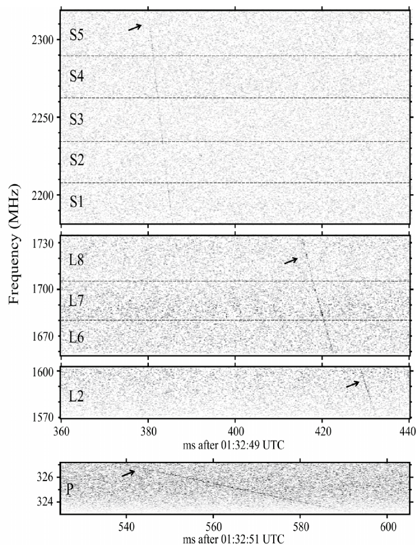
Figure 1.— Dynamic spectra of the GRP #2677, which occurred at 01:32:49-51 UTC on 2014 September 7. This GRP occurred at the main pulse phase.

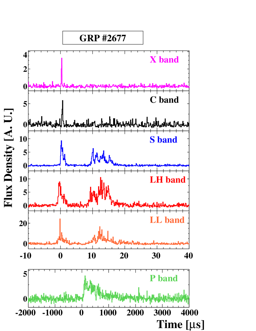
Figure 2.— Dedispersed light curves of the GRP #2677 (same GRP as that shown in Figure 1), which is simultaneously detected at all the bands. The curve in the P band is smoothed with $10\ \mu$s time-bin. The other curves are smoothed with $125$ ns. The spectrum of this GRP is shown in Figure 16.

2.1. Systematic search of GRPs

Below, we describe our methods of GRP search. To extract real GRPs, we set two criteria for the GRP selection: (1) a peak signal-to-noise ratio (S/N) value of dedispersed data exceeds the threshold S/N tabulated in Table 1, and (2) the signal appears at the rotational phase of the main pulse or interpulse.

We smoothed the time series of the dedispersed data for each channel with time resolutions $\Delta t$ tabulated in Table 1, which are adjusted to draw the typical GRP light curve with a few time-bins. From off-pulse phases, we obtained the noise flux, which is mainly due to the Crab nebula background. Based on the noise level and fluctuation, we calculated the S/N of the time series of the data. In order to improve the S/N and mitigate the effects of the interstellar scintillation (see Section 2.2), the data from L6 to L8 channels, and the data from S1 to S5 channels were merged taking into account the overlaps of the frequency intervals of those channels. Hereafter, we call those merged frequency bands “LH band” and “S band”, respectively. We also treat the L2 (hereafter, “LL”) band separately from the LH band, because the frequency separation between the L2 and the L6 bands is larger than their bandwidths.

RFI and statistical fluctuations of the noise give rise to fake signals. The thresholds S/N for the GRP selection (hereafter, “selection thresholds”) were determined to collect as many GRPs as possible and to avoid contamination of fake GRPs. The GRP candidates, whose peak S/N values exceed the selection thresholds, are plotted in Figure 3, where the peak time of the main pulse in LL–S bands is defined as 0.5 in the rotational phase. For P, LL, LH, and S bands, the phase ranges defined to accept signals as GRPs were empirically determined from the distribution of the GRP candidates in our samples. For LL, LH, and S bands, the phase widths are 0.03 rotational period centering at the peak phases for both the main pulse and interpulse phase ranges. The width for the P band is a 0.05 rotational period. At C and X bands, the number of the candidates is too small to determine the phase ranges for the GRP selection. We adopted the same phase ranges as those at S band for the main pulse. For the interpulse phase, we shift the central position 0.015 rotational period earlier than that in S band with a width of 0.06 rotational period following the results of Cordes et al. (2004), who reported that the occurrence phases of GRPs shift $\sim 0.03$ period earlier at above $\sim 4$ GHz. Even in the other phase ranges so-called HFC1/2, Jessner et al. (2005) and Mickaliger et al. (2012) reported the detections of GRPs at X band (however, see Cordes et al., 2004). Though the HFC GRPs are worth investigating, the wide phase range and its low occurrence rate make it difficult to distinguish real GRPs from fake signals due to RFI in our samples. We do not discuss HFC GRPs in this paper.

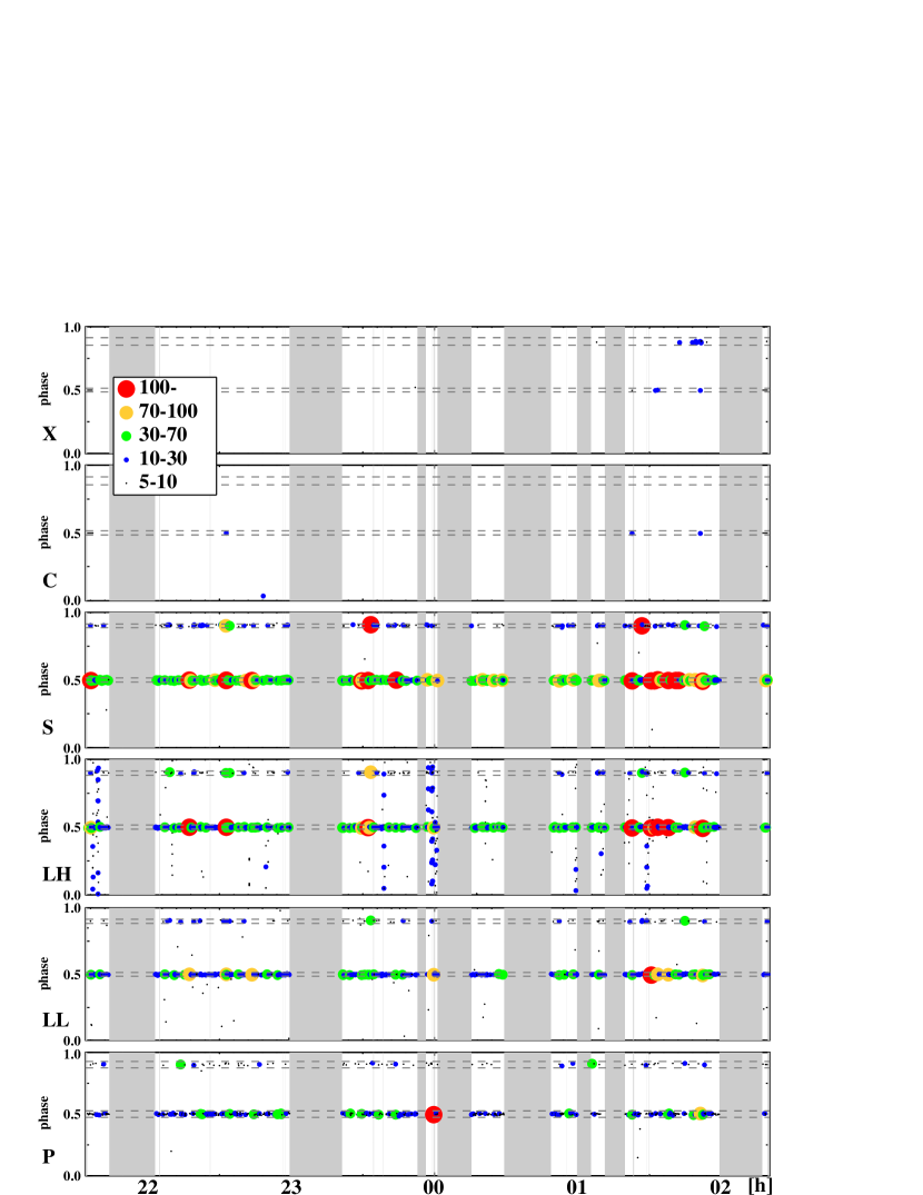
Figure 3.— Scatter plots of phase and time for the GRP candidates from 21^h30^m on 2014 September 6th to 02^h20^m on 2014 September 7th for all the frequency bands. The gray shaded areas are the excluded periods: the calibration observation or the period heavily affected by RFI. The GRP selection phases are denoted by the horizontal dashed lines.

Some candidates appearing outside the defined phases are identified as fake signals. We estimate the expected number of the fake signals appearing accidentally at the GRP selection phases. The expected number of such contamination is at most $\sim 5.2\pm 2.3$ (at the LH band, the errors are estimated assuming that the fake signals follow the Poisson statistics.) during the entire time of the simultaneous observation at all the observatories (see Table 2). The contamination is almost negligible compared to our sample number ($\sim 3000$). The fake signal numbers for C and X bands are very sensitive to the threshold S/N, so that we need to set a relatively higher S/N for the selection threshold in those bands as shown in Table 1.

Table 2Expected number of fake signals appearing accidentally at the GRP selection phases during entire time of the simultaneous observation.

Frequency	Number
Band
X	$9.9\times 10^{-2}$
C	$9.9\times 10^{-2}$
S	$0.45$
LH	$5.2$
LL	$2.5$
P	$1.0$

As a result, we obtained 3194 GRPs occurring at the main pulse phase (hereafter MPGRPs), and 272 GRPs occurring at the interpulse phase (hereafter IPGRPs) during the effective observation time of 2.9 hr. Only 5 MPGRPs and 19 IPGRPs exceeds the selection thresholds at C and/or X band(s). All of those 5 MPGRPs were simultaneously detected at lower frequency bands (P–S). In contrast, all the 19 IPGRPs were detected only at X band.

2.2. Scintillation Effects

Extrapolating the data in Figure 3 of Rickett & Lyne (1990), the timescales of the refractive interstellar scintillation (RISS) are estimated to be about 12 hr or longer for the frequency range lower than $\sim 2$ GHz. Therefore, at these frequency bands, the intensity modulation due to the RISS can be almost negligible during our about 5 hr simultaneous observing session. In contrast, the RISS timescales for C and X band observations are about one hour so that the pulse flux could be modulated during our observing session. Indeed, in the 8.9 GHz observation of the Crab pulsar, Bilous et al. (2011) showed that the numbers of the detected GRPs during two observing sessions of 2 hr in the same day were quite different. This variation of the detection rate may be due to the RISS rather than the intrinsic variation of the GRP activity. In our observation at C or X band, a cluster of GRP candidates can be also seen around 01^h30^m on September 7 (see Figure 3). Therefore, the fluences at our C and X bands may be affected by the RISS.

As for the diffractive interstellar scintillation (DISS), Cordes et al. (2004) measured the scintillation bandwidths as $<0.024$ MHz, $<0.8$ MHz, and $2.3\pm 0.4$ MHz at 0.43, 1.48, and 2.33 GHz, respectively. In our observation at P, L, and S bands, they are at least an order of magnitude smaller than our bandwidths of the frequency channels (see Table 1). The scintillation modulation is presumed to be averaged out at those frequency bands . Also, at L and S bands, the synthesis procedure of the multiple channels described in Section 2.1 may reduce the effect of the DISS. In contrast, extrapolating the result in Cordes et al. (2004) with $\nu^{4.4}$ scaling (corresponding to the Kolmogorov spectrum for the interstellar electron density fluctuation), the scintillation bandwidths for C and X bands are larger than the observation bandwidths. Therefore, the fluences at our C and X bands may be significantly affected by the DISS. Indeed, in the observation by Cordes et al. (2004), the mean pulse flux density was deeply modulated on timescales as short as five minutes at frequencies $\gtrsim 3$ GHz.

As we described above, the fluences at P–S bands may be less affected by the interstellar scintillation so that the fluences in this frequency range are relatively reliable compared to the fluences at the higher frequency bands. Therefore, we first discuss the spectra at P–S bands in Section 3, and then show the spectra including the fluences at C and X bands in Section 4.

2.3. Fluence Estimate

Hereafter, we focus on the time-integrated flux (fluence) of the GRPs rather than the peak flux, because the scatter broadening of the pulse profile depends on frequency (e.g. Cronyn, 1970). In our samples, the GRP durations at LL–X bands distribute widely, while the typical one is $\sim 2\ \mu$s. The P-band pulse profiles show a typically $\sim 1$ ms extent. When we estimate the fluences, we generate time-series of the S/N values with 1 $\mu$s time bin for LL–X bands, and $500\mu$s time bin for P band. Then, the S/N values of all the frequency bands are transformed to the flux density calibrated by reference sources such as Cas A, Cyg A, and so on. In the calibration procedure, we also estimate a received fraction of the flux density from the background nebula taking into account the sizes of the antenna beam and the nebula, and the spatial intensity profile of the nebula. The details of the calibration procedure are described in Appendix A. In the time integration procedure to obtain the fluence $F$, a too long time interval compared to the actual duration of a GRP leads to an excessively large error. We set the time interval individually for each GRP to contain the entire pulse sufficiently. The details to determine the time interval are summarized in Appendix B. Since the sample numbers in C and X bands are small, we do not establish a systematic way to determine the time interval for those bands. The intervals determined manually will be explicitly shown in the light curves in Section 4. As long as a GRP is selected in a certain band with the method described in Section 2.1, the fluences or their upper-limits are estimated for all the bands.

Figure 4 shows the fluence histograms $dN/dF$ of MPGRPs for the P, LL, LH, and S bands. Representing the fluence distribution by a power law $dN/dF\propto F^{\Gamma}$ for the high-fluence portion, the index $\Gamma$ obtained at each band is shown in Table 3. The obtained indices $\Gamma$ are consistent with the previous studies (e.g. Mickaliger et al., 2012).

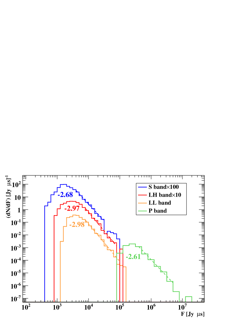
Figure 4.— Fluence histograms $dN/dF$ of MPGRPs in the four bands P, LL, LH, and S. Dashed lines show the fitted power-law function $\propto F^{\Gamma}$. The numbers in the figure are corresponding $\Gamma$.

Table 3Power-law index $\Gamma$ for the fluence distribution.

Band	$\Gamma$ (Sample Number)
	MPGRP	IPGRP
P	$-2.61^{+0.13}_{-0.15}$ (760)	$-2.73^{+0.55}_{-0.83}$ (101)
LL	$-2.98^{+0.11}_{-0.12}$ (2166)	$-2.88^{+0.37}_{-0.50}$ (171)
LH	$-2.97^{+0.13}_{-0.15}$ (2574)	$-2.75^{+0.72}_{-0.87}$ (192)
S	$-2.68^{+0.11}_{-0.13}$ (2681)	$-3.62^{+0.55}_{-0.70}$ (192)

3. GRP Spectra from P to S Bands

In Figures 5 and 6, we show some examples of the spectra. Here, we examine what fraction of the wide band spectra in our samples are consistent with single power laws (hereafter SPLs). The GRP spectra are fitted by the SPL as a function of frequency $\nu$,

$$F(\nu)=F_{0.3}\left(\frac{\nu}{325.1\mathrm{MHz}}\right)^{\alpha},$$ (2)

with a normalization parameter $F_{0.3}$ and index $\alpha$. The goodness-of-fit test is done by means of the $\chi^{2}$ statistic. All the fluences from P to S bands are not always determined. Even if upper limits are included in some frequency bands, we can test the consistency with a SPL for each GRP by the modified $\chi^{2}$ statistic as

$$\hat{\chi}^{2} = \sum_{i}\chi_{i,{\rm det}}^{2}+\sum_{j}\chi_{j,{\rm UL}}^{2}.$$ (3)

For the band $i$, where a certain fluence $F_{i}$ is determined, its contribution to the $\chi^{2}$ statistic is written as

$$\chi_{i,{\rm det}}^{2} \equiv \left(\frac{F_{i}-F(\nu_{i})}{\sigma_{i,{\rm tot}}}\right)^{2},$$ (4)

where $\sigma_{i,{\rm tot}}$ is the $1\sigma$ total error for the given time interval in the band $i$ (see Appendix A). For the band $j$, where a fluence upper limit $F_{j,{\rm max}}$ (see Appendix A) is set, its contribution is

$$\chi_{j,{\rm UL}}^{2} \equiv -2\ln\int_{-\infty}^{F_{j,{\rm max}}}\frac{\exp\left(\frac{-\left(F^{\prime}-F(\nu_{j})\right)^{2}}{2\sigma_{j,{\rm tot}}^{2}}\right)}{\sqrt{2\pi\sigma_{j,{\rm tot}}^{2}}}dF^{\prime},$$ (5)

(Avni et al., 1980; Sawicki, 2012).

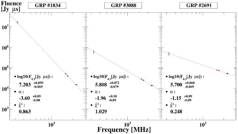
Figure 5.— Examples of the GRP spectra consistent with SPLs. The best-fit power-law functions are plotted with the dotted lines. The obtained parameters with 68% confidence intervals and the minimum $\hat{\chi}^{2}$ are also shown.

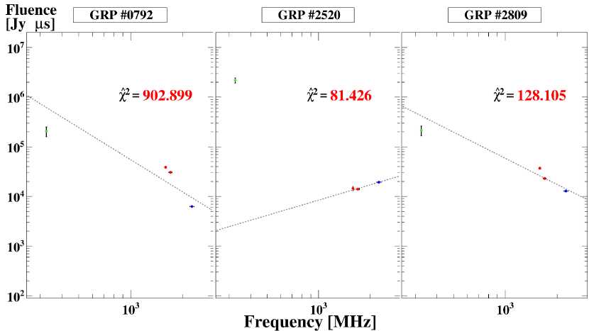
Figure 6.— Examples of the GRP spectra inconsistent with SPLs: hard-to-soft (left), soft-to-hard (middle), and other (right) spectra. The minimum $\hat{\chi}^{2}$ values and corresponding SPL functions (dotted lines) are shown.

We set a critical value of $\hat{\chi}^{2}$ to reject the SPL hypothesis assuming that $\hat{\chi}^{2}$ follows a $\chi^{2}$ distribution with $n-2$ degrees of freedom (DoFs) for $n$ data points. In the case of the spectra for P–S bands, the number of the data points implies $2$ DoFs for $\chi^{2}$ distribution. We adopt a critical value of $\hat{\chi}^{2}=5.99$ (significance level of 5%).

For the GRPs whose spectra are consistent with SPLs, we estimate the confidence intervals or the upper-limits of the fitting parameters as follows. For each pair of the parameters $(F_{0.3},\alpha)$, we calculate $\hat{\chi}^{2}$, and express

$$\hat{\chi}^{2}=\hat{\chi}^{2}_{\rm{min}}+\Delta\hat{\chi}^{2},$$ (6)

where $\hat{\chi}^{2}_{\rm{min}}$ is the minimum value of $\hat{\chi}^{2}$. According to Lampton et al. (1976), we assume that $\Delta\hat{\chi}^{2}$ follows a chi-square distribution with $p$ DoFs, where $p$ is the number of fitting parameters. A 68% confidence interval of each fitting parameter is that satisfying

$$\Delta\hat{\chi}^{2}=2.3,$$ (7)

for $p=2$ in our case.

First, we focus on the GRPs detected at all the four frequency bands. The fractions of such ideal samples are relatively small, 8.4% and 18% for MPGRPs and IPGRPs, respectively (see Table 4). In those samples, we find that 86 of 268 (32%) MPGRPs, and 27 of 46 (59%) IPGRPs are consistent with SPL spectra at a significance level of $5\%$. The spectral index widely distributes between $\sim-4$ and $\sim-1$ (see Figures 5 and 10), while the spectral index of the normal main pulse and interpulse are $-3.0$ and $-4.1$, respectively (Moffett & Hankins, 1999). GRP spectra may show a wider variety in their indices than those of normal pulses. If the significance level is set to 0.1% ($\hat{\chi}^{2}<13.82$), 143 (53%) MPGRPs, and 35 (76%) IPGRPs are consistent with SPL spectra. Furthermore, the goodness of fit depends on the method of the error estimate. When we impose more conservative errors on the fluences (Method B, see Appendix C), the fraction of the consistent spectra with SPLs becomes $\sim 90\%$. Even in the ideal samples, we do not find any strong evidence that the majority of the GRP spectra have a spectral break or multiple components.

3.1. Detection Category

In most of our samples, the fluence data points in the given four bands include several upper-limits. As described below, we categorize our GRPs into the three groups according to the detection/non-detection in the individual bands. Since we focus on the wide-band spectra, we do not discriminate LL and LH bands in the detection category. The GRPs detected at LL and/or LH bands are categorized as GRPs detected at L band.

The GRPs in Group (I) are detected at multiple frequency bands including P band. For Group (I) GRPs, the parameters $F_{0.3}$ and $\alpha$ are determined more precisely than the GRPs in the other groups. An example of the $\hat{\chi}^{2}$-map of the GRPs in Group (I) is shown in the top panel of Figure 7.

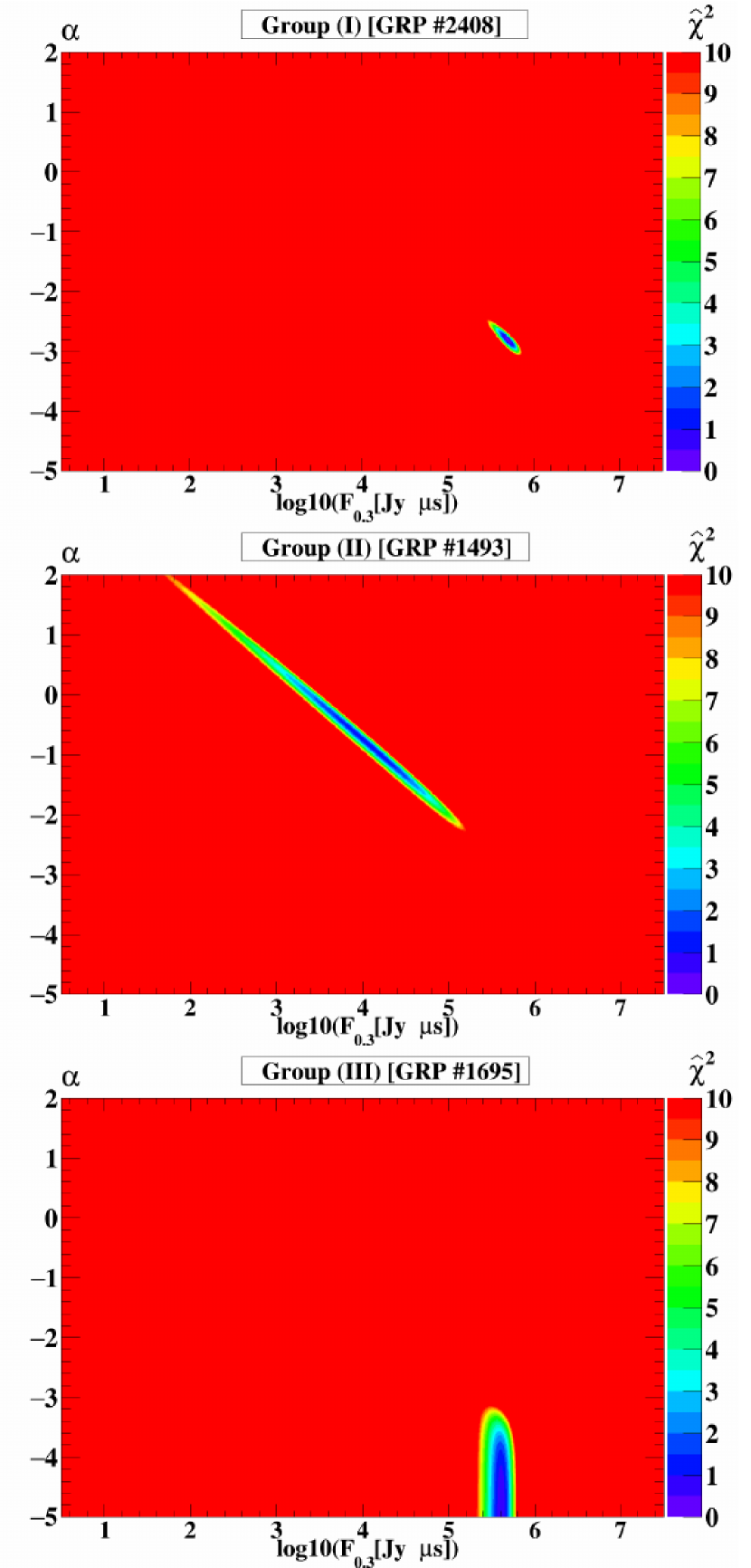
Figure 7.— Behavior of $\hat{\chi}^{2}$ in the parameter space ($F_{0.3},\alpha$) for the typical GRPs in Groups (I)–(III) (see Section 3.1).

Group (II) is defined as the GRPs detected at both L and S bands, but not detected (set an upper-limit) at the P band. For those GRPs, the P-band fluence is estimated by extrapolation using the fluences at L and S bands. For the samples consistent with SPLs in Group (II), of course, the extrapolated value does not conflict with the upper-limit at the P band. As shown in the middle panel of Figure 7, the typical allowed region in the parameter space for Group (II) GRPs is obliquely elongated. In this case, the spectral index is loosely determined because of the relatively narrow frequency separation between L and S bands.

The GRPs detected at P band, but neither L nor S band, belong to Group (III). For those GRPs, while the fluence at P band, $F_{0.3}$, is precisely determined, the upper-limits at higher frequency bands merely provide an upper-limit on $\alpha$. The $\hat{\chi}^{2}$-map in the bottom panel of Figure 7 shows the allowed region is vertically elongated. In this case, we set $\hat{\chi}_{\rm{min}}^{2}=0$. Then, we set the 68% upper limit of $\alpha$ as the maximum value of $\alpha$, satisfying $\Delta\hat{\chi}^{2}=\hat{\chi}^{2}=2.3$.

3.2. Test of SPL hypothesis

Table 4The numbers of GRPs divided according to the detection/non-detection in the individual bands. The samples are classified with the consistency with SPL spectra as well.

		SPL Hypothesis (MPGRP)			SPL Hypothesis (IPGRP)
Detection Y/N	Groupa	Consistent	Inconsistent		Consistent	Inconsistent
(P, LL, LH, S band)		($\hat{\chi}_{\mbox{min}}^{2}<5.99$)	($\hat{\chi}_{\mbox{min}}^{2}>5.99$)		($\hat{\chi}_{\mbox{min}}^{2}<5.99$)	($\hat{\chi}_{\mbox{min}}^{2}>5.99$)
(Y, Y, Y, Y)	I	86	182		27	19
(Y, Y, Y, N)	I	0	3		0	0
(Y, N, N, Y)	I	0	1		0	0
(Y, Y, N, Y)	I	0	0		0	0
(Y, N, Y, Y)	I	5	11		1	1
(Y, Y, N, N)	I	0	0		0	0
(Y, N, Y, N)	I	0	0		0	0
(N, Y, Y, Y)	II	1230	619 ($\alpha>2$ : 9)		88	34
(N, Y, N, Y)	II	13	7		0	0
(N, N, Y, Y)	II	342	60 ($\alpha>2$ : 4)		15	1
(N, Y, Y, N)	$\cdots$	0	24		0	1
(N, N, N, Y)	$\cdots$	103	22 ($\alpha>2$ : 22)		6	0
(N, Y, N, N)	$\cdots$	0	2		0	2
(N, N, Y, N)	$\cdots$	1	11		0	5
(Y, N, N, N)	III	471	1 ($\alpha<-5$ : 1)		52	1 ($\alpha<-5$ : 1)
Total		2251	943		189	64
			($\alpha>2$ : 35, $\alpha<-5$ : 1)			($\alpha>2$ : 0, $\alpha<-5$ : 1)

a: We categorize the GRPs into three groups, from I to III. See Section 3.1.

The numbers of the GRPs divided according to the consistency of their spectra with SPLs, are summarized in Table 4 and Figure 8. In this analysis, GRP samples with an extreme spectral index, $\alpha>2$ or $<-5$, are excluded from the SPL samples even if the $\hat{\chi}^{2}$-value is small enough. Such examples are shown in Figure 9. We find that the spectra of 2251 of 3194 MPGRPs (70.5%) and 189 of 253 IPGRPs (74.7%) are consistent with SPLs at a significance level of 5%. We show the histograms of the spectral indices sorted by $F_{\rm P}$ or $F_{0.3}$ in Figure 10. Their mean spectral indices of them are also shown in Table 5.

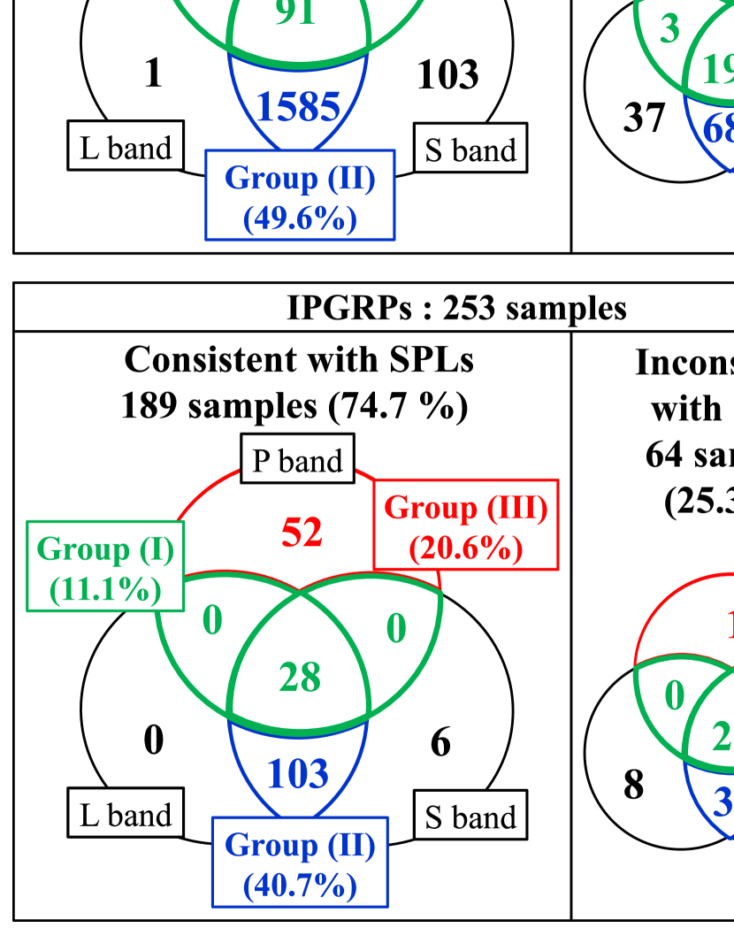
Figure 8.— Categorization of our spectral samples. The numbers in the regions, where circles overlap each other mean the number of GRPs detected at corresponding multiple bands. The GRPs detected at LL band and/or LH band are merged into the category of the “L band” detection. See also Table 4.

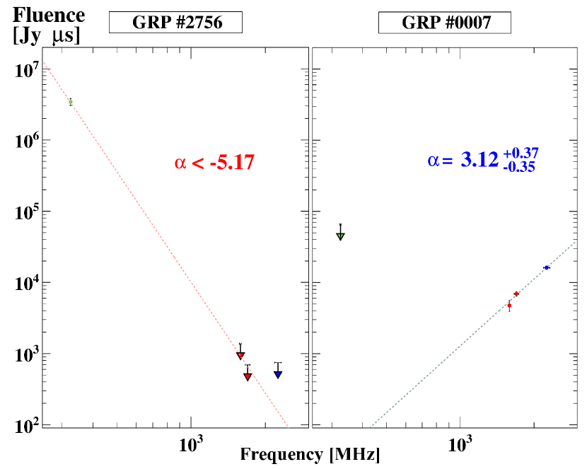
Figure 9.— Examples of the spectra of the ”ultra-soft” (left) and the ”ultra-hard” (right) GRPs. For the ultra-soft GRP, the SPL function with the 68% confidence upper-limit of $\alpha$ is plotted with the dotted line. Also for the ultra-hard GRP, the best-fit SPL function is plotted.

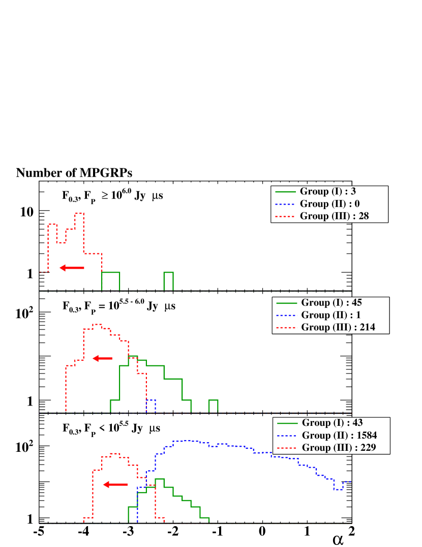
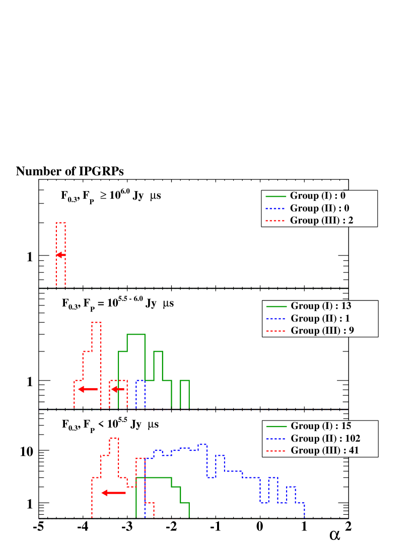
Figure 10.— Histograms of the spectral index $\alpha$ for the MPGRPs (left) and IPGRPs (right). Each panel is divided according to the fluence at P band: $(F_{0.3},F_{\rm P})\geq 10^{6}\mathrm{Jy}~{}\mu\rm{s}$ (top), $10^{5.5}\mathrm{Jy}~{}\mu\rm{s}\leq(F_{0.3},F_{\rm P})<10^{6}\mathrm{Jy}~{}\mu\rm{s}$ (middle), and $(F_{0.3},F_{\rm P})<10^{5.5}\mathrm{Jy}~{}\mu\rm{s}$ (bottom). The errors in $\alpha$ are neglected, and the histogram of Group (III) represents the upper-limit values; i.e. the histograms with dashed lines (Group (II) and (III)) implies that the values $\alpha$ are not determined firmly.

Table 5Mean spectral index $\alpha$ sorted by $F_{\rm P}$ or $F_{0.3}$.

$F_{\rm P}$ or $F_{0.3}$	Group	$\alpha$
		MPGRP		IPGRP
	I	$-3.03\pm 0.61$		$\cdots$
$\geq 10^{6.0}$ Jy $\mu$s	II	$\cdots$		$\cdots$
	III	$<-3.66$		$<-4.49$
	I	$-2.58\pm 0.44$		$-2.61\pm 0.40$
$10^{5.5}-10^{6.0}$ Jy $\mu$s	II	$-2.59$		$-2.61$
	III	$<-2.68$		$<-3.06$
	I	$-2.23\pm 0.37$		$-2.29\pm 0.31$
$<10^{5.5}$ Jy $\mu$s	II	$-0.91\pm 0.98$		$-1.38\pm 0.82$
	III	$<-2.34$		$<-2.59$
	I	$-2.44\pm 0.47$		$-2.44\pm 0.38$
ALL	II	$-0.91\pm 0.98$		$-1.39\pm 0.82$
	III	$<-2.34$		$<-2.59$

Note that our result does not necessarily imply that remaining $\sim 30$% of the GRP spectra totally deviate from an SPL. As we mentioned before, the goodness of fit depends on the method of the error estimate (see Appendix C). Although we cannot conclude that the majority of GRP spectra are definitely SPLs, there is no strong evidence that rejects SPLs as the typical spectral shape. In Sections 3.3 and 3.4, we discuss the GRP spectra consistent with SPLs, and then discuss the inconsistent ones in Section 3.5.

3.3. The P-band Fluence and Hardness

Similarly to the result in Sallmen et al. (1999), we do not find a significant correlation between the fluences at P and L bands. This suggests that the spectral index distributes widely. We investigate the distributions of the index $\alpha$ as a function of the fluence below.

Since the most of the radiation energy is released at P band or lower frequencies for an SPL GRP with $\alpha<-1$, we focus on the P-band fluence here. For the samples consistent with SPLs, we show the scatter plots in the parameter space of SPL in the central panel of Figures 11 and 12 for the MPGRPs and IPGRPs, respectively. In those figures, we plot the observed fluences $F_{\rm P}$ for Groups (I) and (III), while the values $F_{0.3}$ estimated from Equation (2) are plotted for Group (II). With the 68% confidence interval, the errors in the figures are plotted in the standard manner for Group (I), but the confidence region ellipses (Press et al., 1992) are directly drawn for Group (II). This is because the allowed regions for Group (II) are inclined and elongated, as shown in the middle panel of Figure 7, reflecting the fact that the value of $F_{0.3}$ estimated from extrapolation largely depends on $\alpha$. For Group (III), we plot the upper limits on $\alpha$ with the observed $F_{\rm P}$.

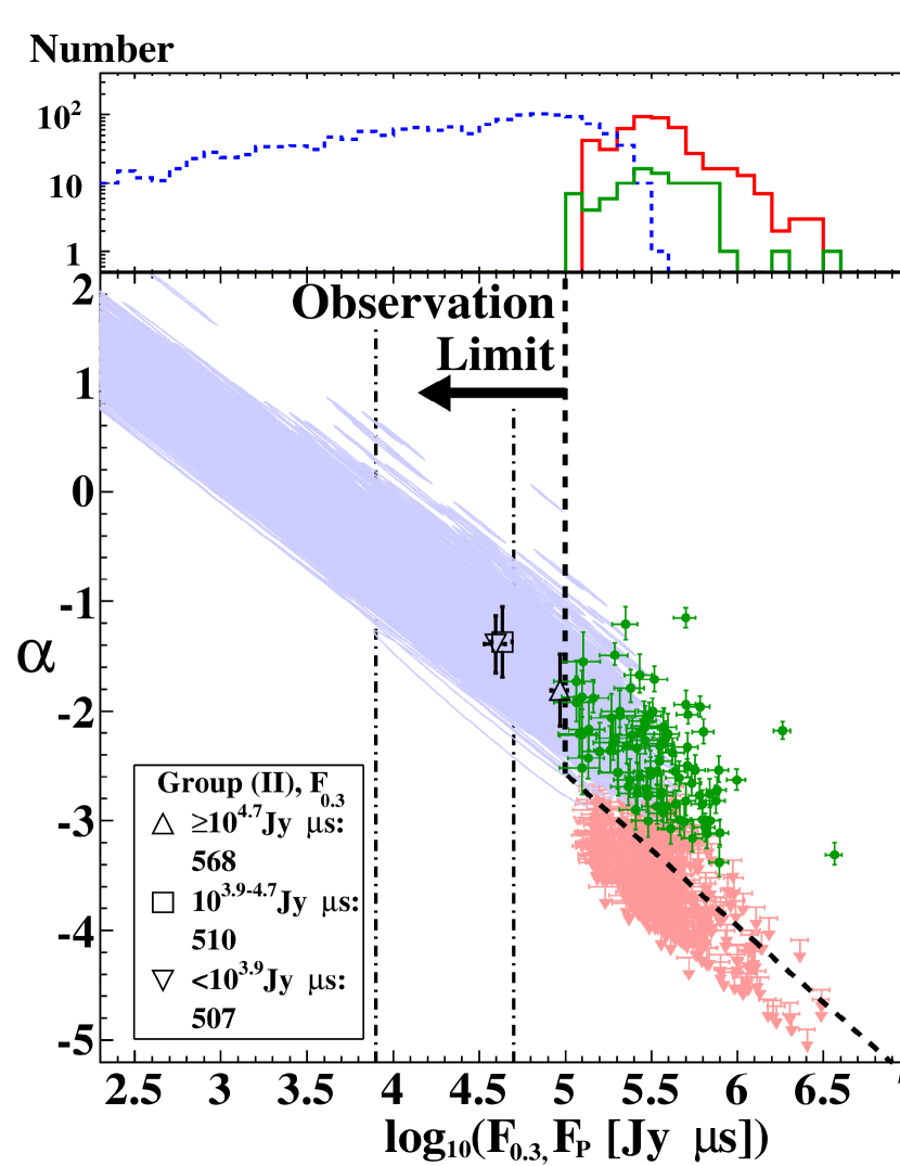
Figure 11.— Scatter plot of the observed/extrapolated P-band fluences and the spectral indices $\alpha$ for the MPGRPs whose spectra are consistent with SPLs. The data for Groups (I), (II), and (III) are shown with green, blue, and red symbols, respectively. The upper-left and the lower-right panels are the number distributions for the parameters of their axes, where we put samples into a bin neglecting the errors. Note that the $\alpha$-histogram for Group (III) consists of the upper-limit values. In the upper-right panel, $R$ is the Spearman rank correlation coefficient for Group (I). The dashed lines represent the observation limit to judge a GRP as one of Group (I). By the vertical dash-dotted lines in the central panel, we further divide the samples in Group (II) into three sub-groups. The average values of $F_{\rm P}$ and $\alpha$ ($\bar{F}_{\rm{stk}}$ and $\bar{\alpha}_{\rm{est}}$) obtained with the stacking analysis for each sub-group are plotted with the open triangles and the square (see Section 3.3 and Table 6).

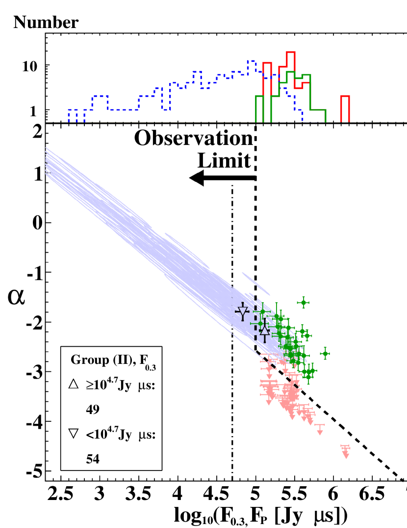
Figure 12.— Same plot as Figure 11, but for the IPGRPs.

At a glance, the scatter plots seem to show a correlation between the hardness and fluence. Figure 10 also seems to show the tendency of softening with increasing fluence (brighter–softer). However, we should take into account the observational bias. In the scatter plots, we also draw the rough “observation limit” lines (the limit depends on the pulse duration technically) indicating the regions where the fluence at P or LH band is below the detection limit. This limit corresponds to the necessary condition to classify an SPL-GRP into Group (I). In the scatter plots, dimmer and softer GRPs are not found in the lower-left region. Such GRPs are also expected to be dim at L/S bands so that the deficit of GRPs in that region can be due to the observation bias. On the other hand, the brighter and harder (the upper-right region) GRPs are expected to be easily detected at the L/S band as long as the spectrum extends. We extract only the samples in Group (I) (green points), whose parameters are determined most accurately, and calculate the Spearman rank correlation coefficient, $R$ (e.g. Press et al., 1992). The values of $R$ are $-0.53$ for the MPGRPs and $-0.67$ for the IPGRPs. From the values of $R$, the probabilities that those two variables are unrelated (hereafter $p$-value) are $7\times 10^{-8}$ for MPGRPs, and $1\times 10^{-4}$ for IPGRPs. However, the observational limit, denoted with the inclined lines, may affect those values.

It is also seen from those scatter plots that, whereas the samples in Group (II) imply an existence of a significant number of hard GRPs ($\alpha\gtrsim-1$), there are not many hard GRPs in Group (I) (see also Figure 10). The Group (II) GRPs are not detected at P band consistently with the estimated hard spectral index. This also seems to support the apparent correlation, brighter–softer or dimmer–harder. Since the fluences at P band for Group (II) are extrapolated values, it is worth confirming whether the average flux after stacking over the corresponding GRP intervals exceeds the normal pulse flux. We collect the light curves at the P band in the rotational periods when Group (II) GRPs occurred. According to the extrapolated values of $F_{0.3}$, the MPGRPs are divided into three sub-groups with two boundary values at $F_{0.3}=10^{3.9}$ and $10^{4.7}$Jy $\mu$s. Similarly, the IPGRPs are divided into two sub-groups with a boundary value at $F_{0.3}=10^{4.7}$Jy $\mu$s. These boundary values are chosen so as to make the sub-groups of similar size (Table 6).

The resultant average pulse profiles are shown with the colored lines in Figure 13. Compared to the average pulse profile of the off-GRP periods, it is clearly seen that the pulse at the P band is on average enhanced at the GRP period defined with L/S bands. The average fluences $\bar{F}_{\rm{stk}}$ and $\bar{F}_{\rm{off}}$ for on- and off-GRP periods, respectively, are evaluated for phase intervals shown with the arrows in Figure 13. The width of the intervals is 0.11 period, which is the sum of the width for the GRP selection (0.05 period) and the characteristic duration of the GRPs at the P band ($\sim 2$ms, 0.06 period). The calculated values of $\bar{F}_{\rm{stk}}$ and $\bar{F}_{\rm{off}}$ are summarized in Table 6. From $\bar{F}_{\rm{stk}}$ and the fluence $F_{\rm{S}}$ of each GRP at S band, we deduce average spectral indices $\bar{\alpha}_{\rm{est}}$ as

$$\bar{\alpha}_{\rm{est}}\equiv\frac{1}{N_{\rm{GRP}}}\sum_{i}^{N_{\rm{GRP}}}\frac{\log{(\bar{F}_{\rm{stk}}/F_{\rm{S},i}})}{\log{(325.1\rm{MHz}/2250\rm{MHz})}}.$$ (8)

The values of $\bar{\alpha}_{\rm{est}}$ are also tabulated in Table 6, and $(\bar{F}_{\rm{stk}},\bar{\alpha}_{\rm{est}})$ are plotted in Figures 11 and 12 as the open black symbols. Those average points are consistently on the clusters of the blue ellipses, which are extrapolated from fluences at L and S bands, and seem to reinforce the SPL hypothesis and the tendency of the softening with increasing $F_{\rm P}$, considering the green data points of Group (I). In addition, the obtained values of $\bar{\alpha}_{\rm{est}}$ are significantly larger than the average values for the samples with brighter $F_{\rm P}$, Groups (I) and (III) (see Figure 10 and Table 5), or the index of the normal pulse ($\sim-3$).

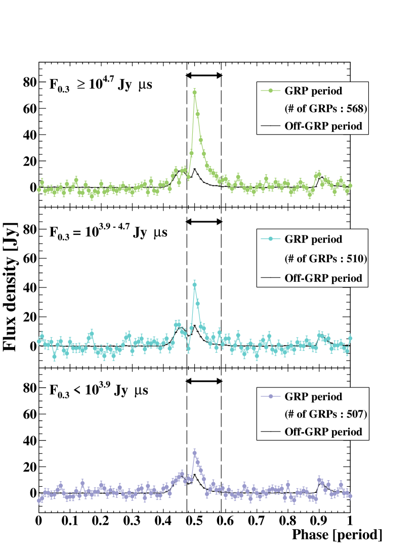
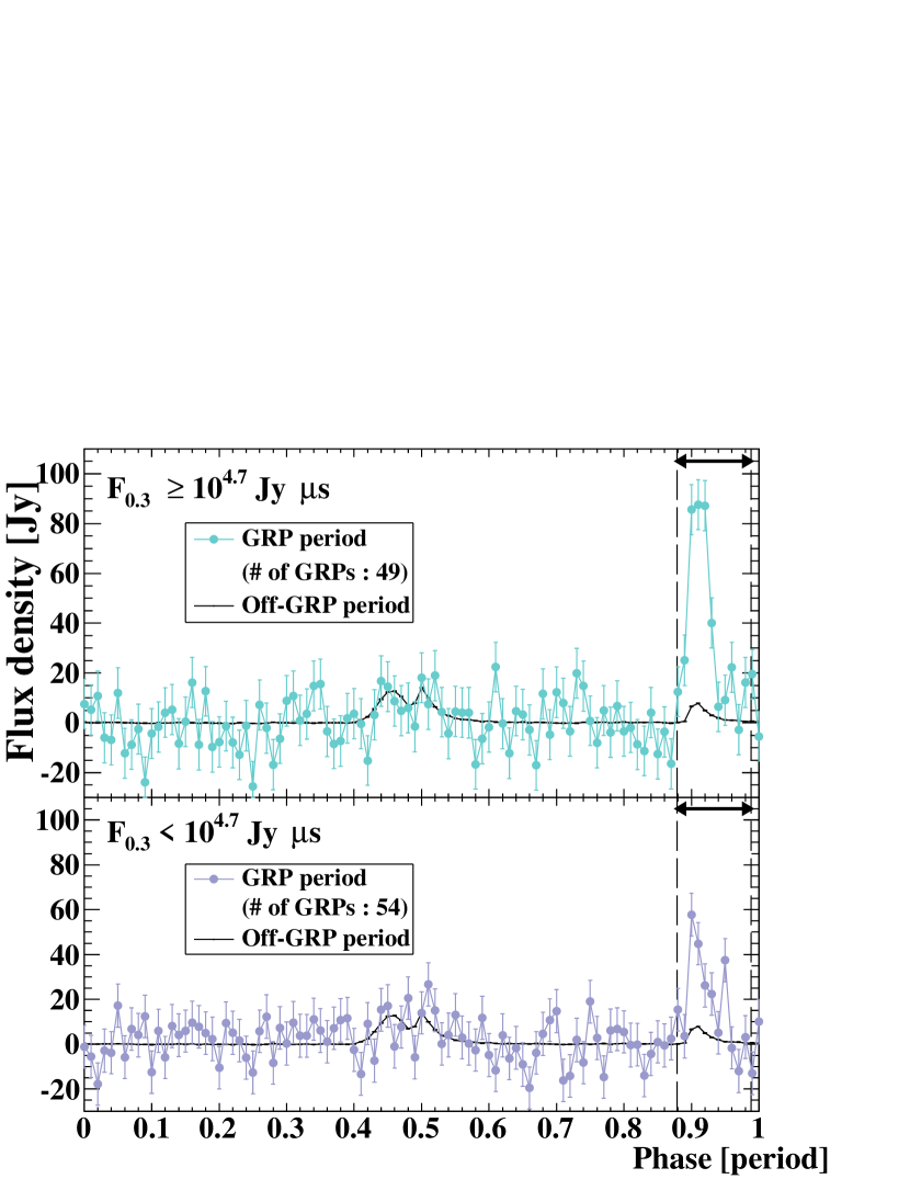
Figure 13.— Average pulse profiles at the P band, when Group (II) MPGRPs (left) and IPGRPs (right) occurred. The samples are divided into sub-groups according to the fluence $F_{0.3}$. We also show the average profile for the off-GRP periods. The $1\sigma$ statistical errors are shown with the error bars. The phase intervals to estimate the fluence are shown by the arrows.

Table 6The mean fluences $\bar{F}_{\rm{stk}}$, $\bar{F}_{\rm{off}}$ and spectral indices $\bar{\alpha}_{\rm{est}}$.

	MPGRP				IPGRP
$\log_{10}F_{0.3}[\rm{Jy~{}\mu s}]$	$\geq 4.7$	$3.9-4.7$	$<3.9$		$\geq 4.7$	$<4.7$
$N_{\rm{GRP}}$	568	510	507		49	54
$\log_{10}\bar{F}_{\rm{stk}}[\rm{Jy~{}\mu\rm{s}}]$	$4.97^{+0.05}_{-0.05}$	$4.64^{+0.05}_{-0.07}$	$4.60^{+0.05}_{-0.07}$		$5.12^{+0.05}_{-0.07}$	$4.83^{+0.08}_{-0.09}$
$\log_{10}\bar{F}_{\rm{off}}[\rm{Jy~{}\mu\rm{s}}]$	$4.28^{+0.05}_{-0.05}$				$3.98^{+0.05}_{-0.05}$
$\bar{\alpha}_{\rm{est}}$	$-1.81\pm 0.33$	$-1.37\pm 0.32$	$-1.39\pm 0.26$		$-2.17\pm 0.24$	$-1.79\pm 0.18$
a. Number of GRP samples.

For the brighter sub-groups of $F_{0.3}\geq 10^{4.7}\rm{Jy}~{}\mu\rm{s}$, the obtained values of $\bar{F}_{\rm{stk}}$ are consistent with the prospective fluence $F_{0.3}$. However, for the dimmer sub-groups, $F_{0.3}<10^{3.9}\rm{Jy}~{}\mu\rm{s}$ for MPGRPs and $F_{0.3}<10^{4.7}\rm{Jy}~{}\mu\rm{s}$ for IPGRPs, the values of $\bar{F}_{\rm{stk}}$ become higher than the corresponding range of $F_{0.3}$. If the SPL hypothesis is correct even for such dimmer GRPs, the above contradiction may be due to the contribution of the normal pulse. Since we have assumed that the normal pulse is absent at the GRP periods, we have not subtracted the contribution of the normal pulse. For such low-fluence GRPs, the method to distinguish GRPs from the normal pulses is not established so far. Another interpretation for the discrepancy between $\bar{F}_{\rm{stk}}$ and $F_{0.3}$ is that non-SPL GRPs are contaminated in Group (II) samples.

3.4. The L/S-band Fluence and Hardness

In the previous subsection, we have found signatures of a possible correlation between the fluence at the P band and hardness. However, the observational bias obscures the conclusion for the correlation. To probe clues about the correlation from another angle, we discuss the correlation between the L/S band fluence and hardness in this subsection.

We choose the GRPs, whose spectra are consistent with SPLs in Group (I) (see Tables 4 and Section 3.1). The uncertainty in the spectral index are relatively low owing to the wide frequency separation between P and L/S bands (see Section 3.1). We show scatter plots of the fluences at LL or S band and the indices $\alpha$ in Figures 14 and 15 for the MPGRPs and IPGRPs, respectively. Since the detection limit becomes deepest at the LH band, the fluence limit at the LL band is the fluence at the LL band for an SPL GRP, whose fluences at LH and P bands are on the detection limit. The apparent correlations between the fluence and hardness are seen clearly. From the Spearman rank correlation coefficients, the $p$-values for the correlation absence described in the previous subsection are $4\times 10^{-8}$ and $3\times 10^{-12}$ for MPGRPs at LL and S bands, respectively. While we have omitted the results for LH band, the results are similar (91 samples, $R=0.57$ for MPGRPs and 28 samples, $R=0.79$ for IPGRPs). The deficit of samples in the upper-left region can be due to the selection bias. However, the deficit in the lower-right region cannot be explained by the selection bias.

Contrary to the case of the P band, a positive correlation between the fluence and spectral hardness is found in the cases of L/S bands. If the negative correlation in the P-band case is real, our results suggest that the fluences at P band and L/S band have an anti-correlation. This is intuitively understood from Figure 5. Since the most of the GRP energy is released at P band or lower frequencies, the anti-correlation means that more energetic GRPs tend to show softer spectra.

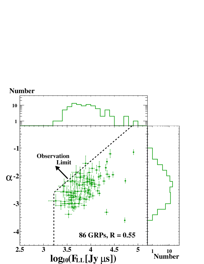
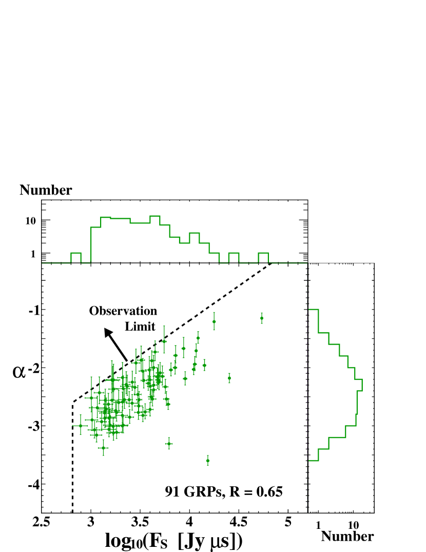
Figure 14.— Scatter plots of the observed fluences at LL (left) and S (right) bands and the spectral indices $\alpha$ for the MPGRPs belonging to Group (I). The distributions of the fluences and indices are projected on the upper and right sides of each panel. The dashed lines represent the observation limit to be detected at both P and corresponding bands. The Spearman rank correlation coefficients $R$ are also shown.

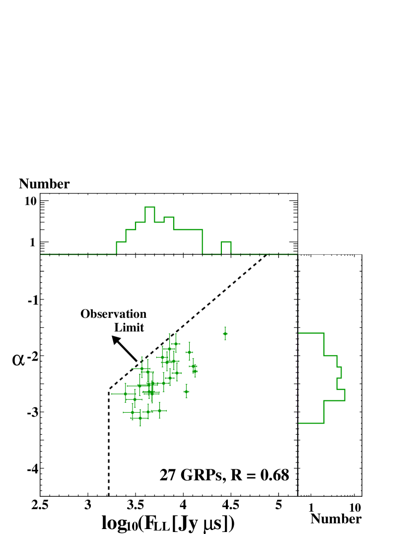
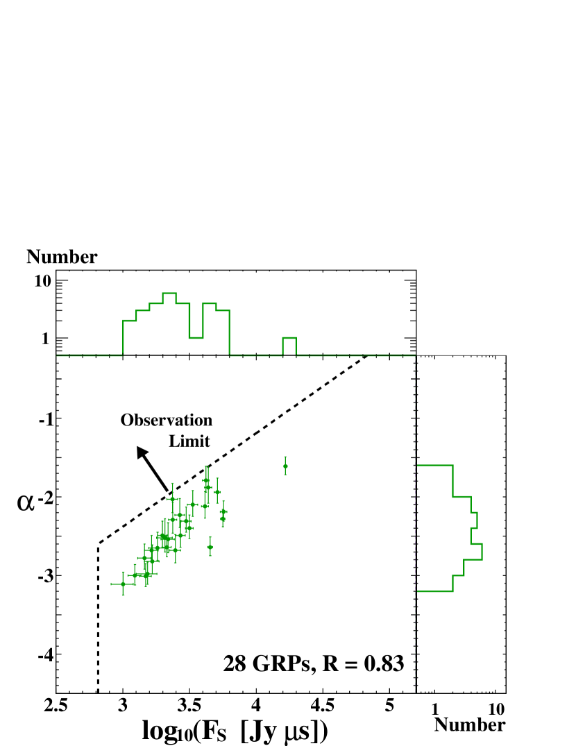
Figure 15.— Same as Figure 14 but for IPGRPs.

We carry out Monte Carlo simulations to reproduce the scatter distributions without an intrinsic correlation between the L-band fluence and hardness (see Appendix D). When we assume that the typical spectral index is close to that of the normal pulse of $-3$, the Spearman coefficient in the $F_{\rm LL}$–$\alpha$ diagram cannot be reproduced. However, if we assume the typical index of $-1$, harder than the normal pulse’s one, the apparent correlations in both the $F_{\rm LL}$–$\alpha$ and $F_{\rm P}$–$\alpha$ are reproduced. This is consistent with the hard spectrum implied from the stacking analysis. Given $F_{\rm LL}$, a smaller $\alpha$ implies a brighter P-band fluence, where most of energy is released. Namely, the uncorrelation between $F_{\rm LL}$ and $\alpha$ is equivalent to an anti-correlation between the total energy release and hardness. Therefore, the apparent correlations in Figures 11, 12, 14, and 15 imply that a more energetic GRP tends to have a softer spectrum. In our samples, the P-band GRPs, including Group (III) GRPs, whose spectrum should be very soft, are energetic samples compared to Group (II) GRPs. The different average $\alpha$ for P band GRPs and Group (II) GRPs also indicates the anti-correlation between the energy release and hardness.

When we add the GRPs in Group (II) for the correlation analysis, a significant correlation is not found. This may be partially due to the large errors in the index of Group (II) GRPs. Alternatively, another type of GRPs, whose spectra are not SPLs may be contaminated in Group (II) samples.

3.5. Inconsistent Spectra with SPLs

The fractions of the GRPs judged to be inconsistent with SPLs at a significance level of 5% are 28.4% and 24.9% for the MPGRPs and the IPGRPs, respectively. When the significance level is set to 0.1% ($\hat{\chi}^{2}<13.82$), the fractions are 14.2% and 14.6% for the MPGRPs and the IPGRPs, respectively. Examples of the spectra apparently inconsistent with SPLs are shown in Figure 6. Some spectra show softening or hardening at higher frequencies. Such hard-to-soft (left), soft-to-hard (center), and other (right) examples are displayed in the figure. Popov et al. (2008, 2009) claimed that GRP spectra tend to show soft-to-hard behavior at 0.6–2.2 GHz. In order to examine this tendency, we choose 182 MPGRPs and 19 IPGRPs that are detected at all the bands from P to S, and are inconsistent with SPL spectra at a significance level of 5%. In those MPGRP samples, the fractions of hard-to-soft, soft-to-hard, and other spectra are 48 (26%), 76 (42%), and 58 (32%), respectively. For the 19 IPGRPs, the numbers are 3 (16%), 4 (21%), and 12 (63%), respectively. We do not find a clear tendency in the spectral behavior.

We find 1 (0.03%) ultra-soft ($\alpha<-5$) and 35 (1.1%) ultra-hard ($\alpha>2$) MPGRPs, and we also find 1 (0.4%) ultra-soft IPGRPs (see Figure 9). In our GRP samples, no ultra-hard IPGRP is found.

4. GRPs Detected at the C/X Band

In this section, we discuss the GRPs detected at C and/or X band(s). Note that the fluences at C and X bands are expected to be affected by intensity modulation due to the interstellar scintillation.

We find 5 MPGRPs and 19 IPGRPs exceeding the selection thresholds (see Section 2.1 and Table 1) at C and/or X band(s). All of these five MPGRPs were simultaneously detected at some of the frequency bands of P, L, or S band. In contrast, all the 19 IPGRPs were detected only at X band. As for the IPGRPs in Groups (I) and (II) discussed in Section 3, the spectra may have a cut-off below the X band frequency.

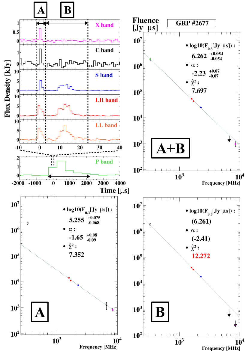
Figure 16.— Spectra of the GRP (upper-right), whose dynamic spectra and pulse profiles are shown in Figures 1 and 2. The spectra for time intervals A and B defined in the upper-left light curve are shown in the bottom panels. The data point at P band is excluded for the fits for the time intervals A and B, respectively.

In Figure 16, we show the spectrum of the MPGRP #2677, whose pulse profiles and dynamic spectra are shown in Figures 1 and 2, respectively. The spectrum is consistent with a SPL at P–X bands at a significance level of 5%. This is only the case consistent with a SPL in the five MPGRPs.

As seen in Figure 16, the light curve shows two distinct components, so that we attempt to obtain the temporally divided spectra here. When we divide the light curve into two intervals A and B defined in Figure 16, it turns out that the spectrum for the interval B needs a high-frequency cut-off. In Figure 2, many finer (sub-$\mu$s) structures (e.g. Hankins et al., 2003) are found in the light curve. The spectrum may consist of further more components as well.

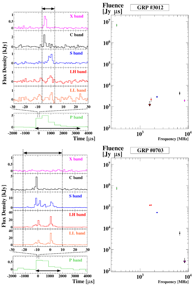
Figure 17.— Examples of broadband GRP spectra (right) inconsistent with SPLs. The pulse profiles (left) are also shown with the time intervals for the integral.

The spectra of the other four MPGRPs are inconsistent with SPLs as shown in Figure 17. The P-band fluence of GRP #3012 is about three orders of magnitude brighter than fluences at the higher frequency bands. The spectrum seems to consist of two or more different components, which may be supported by the slight misalignment of the peak times ($\sim 4\ \mu$s) between the light curves in S and C/X bands. The small uncertainty of the TOA between LL and X bands ($\sim 1.5\ \mu$s) suggests that the $4\ \mu$s misalignment is an intrinsic feature. The pulse profile of GRP #0703 appears to have multiple components (especially at L and S bands), similarly to the GRP #2677 (Figure 16). The stringent upper-limit at the X band requires a sharp high-frequency cut-off in the spectrum. For GRP #0703, the temporally divided spectra are also inconsistent with SPLs and need low/high-frequency breaks or cut-offs.

5. Discussion and Conclusion

The broadband (0.3, 1.6, 2.2, 6.7, and 8.4 GHz) simultaneous observation of the GRPs from the Crab pulsar was conducted with four Japanese observatories, Iitate, Kashima, Usuda, and Takahagi, on 2014 September 6-7th. We obtained 3194 MPGRPs and five of them were detected at the multiple frequency bands including 6.7 and/or 8.4 GHz. We also obtained 272 IPGRPs and 19 of them were detected only at 8.4 GHz. We investigated the spectra of those GRPs. Our results are as follows.

• In the frequency range from P to S bands (0.3–2.2 GHz), 70% or more of the spectra in our GRPs are consistent with SPLs. We do not find a strong evidence that the majority of GRPs disagree with SPL spectra.

• For the GRPs, whose spectra are consistent with SPLs, the spectral index is widely distributed from approximately $-4$ to $-1$.

• The GRP distributions in the fluences at P band and spectral index show a possible negative correlation.

• For the L/S band GRPs, which are not detected at P band, we carry out the stacking analysis of the P-band light curve. We find significant enhancement in the P-band light curves compared to the light curves in the non-GRP periods. This indicates that those L/S-band GRPs accompany dim P-band GRPs. The average spectral indices for those samples, approximately $-1$ or $-2$, are harder than the bright GRPs. This supports the possible negative correlation between the P-band flux and hardness. Since the dim and hard GRPs (Group (II)) occupy about a half of our GRP samples, it might be suggested that most of GRPs may have intrinsically harder spectra than that suggested in the previous studies.

• A positive correlation between the L/S band fluence and hardness is found. Considering the negative correlation at P band, our results suggest an anti-correlation between the total energy release and hardness. Our Monte Carlo simulations to reproduce the distributions of the fluences and $\alpha$ show that the typical spectral index is as hard as $-1$ again.

• We find several ultra-soft ($\alpha<-5$) and ultra-hard ($\alpha>2$) GRPs.

• A small fraction of spectra apparently deviate from SPLs. We do not find any tendency in the spectral shape for such GRPs.

• Several GRPs are detected in a very wide frequency range of $0.3$–$8.4$ GHz. Most of them need multiple spectral components.

5.1. Comparison with the previous studies

Karuppusamy et al. (2010) reported that the distribution of the spectral index is extremely wide (from about $-15$ to $+10$) for a narrow frequency range of 1.3-1.45 GHz. In our observation, the fluences at the four channels in L band significantly fluctuate (see Appendix C). If we fit such data with an SPL, a similar result to Karuppusamy et al. (2010) may be obtained. Such fluctuation might be intrinsic, or due to the scintillation modulation. It should be noticed that a large fraction of our broadband spectra do not conflict with SPLs from P to S bands. Our broadband analysis seems more convincing than the results based on the narrow frequency range.

Sallmen et al. (1999) investigated the spectral index between 0.6 and 1.4 GHz, and obtained their distribution ranging from $-4.9$ to $-2.2$. Although the frequency range is slightly different, the index for Group (I) is distributed within a similar range (see Figure 10). Oronsaye et al. (2015) investigated the spectral index between 0.2 and 1.4 GHz, and obtained their distribution ranging from $-4.9$ to $-3.6$. However, the fluences at 1.4 GHz in Oronsaye et al. (2015) are about two orders of magnitude smaller than those in the previous studies (e.g. Sallmen et al., 1999; Bhat et al., 2008), which are roughly consistent with our values, so that the results in Oronsaye et al. (2015) should be reconsidered.

5.2. Emission Mechanism

Our results suggest the anti-correlation between the total energy release and hardness. The emission mechanism for the broadband GRPs may be different from the anomalous cyclotron resonance model (Lyutikov, 2007) proposed for the characteristic property of the IPGRPs above 4GHz (Hankins & Eilek, 2007), for which we did not detect the signal of the counterpart at P–S bands. In the induced scattering model (Petrova, 2004), the intensity variation is attributed to the fluctuation of the optical depth to the induced scattering. Petrova (2004) suggested that the intensity amplification for the Crab GRPs is more efficient at the lower frequencies, which agrees with the correlation we found. Alternatively, a larger energy release may enhance the efficiency of the electron–positron pair production. The resultant high-density pairs may screen out the electric field relatively soon, which may reduce the fraction of higher energy electrons/positrons. Considering the unstable behavior of the magnetosphere as demonstrated by Timokhin & Arons (2013) or Kisaka et al. (2016), the above simple interpretation can be an option to explain the correlation. In any case, before jumping to a conclusion, we need to examine various nonlinear processes in the GRP activity such as the detailed properties of the charge bunching due to two stream instability (Cheng & Ruderman, 1980) and the photon softening due to the induced Compton scattering (e.g. Tanaka et al., 2015).

5.3. Comparing with FRBs

Extremely bright GRPs from young pulsars are candidates of the emission process for FRBs (e.g. Cordes & Wasserman, 2016; Connor et al., 2016). The measured spectrum indices of FRBs are from $\sim-4$ to $\sim+1$ (Lorimer et al., 2007; Keane et al., 2012; Ravi et al., 2015; Keane et al., 2016), which are roughly consistent with that of Crab GRPs. One exception is the repeating FRB 121102, whose range of the spectrum index is extremely wide, from $\sim-10$ to $\sim+14$ (Spitler et al., 2016). Although such hard and soft bursts may correspond to the ultra-hard and ultra-soft GRPs in our samples (Figure 9), this wide range of the spectral index may be due to the narrow frequency range (1.2–1.5GHz) in their observation. In fact, if we obtain the spectral index distribution from fluences in LL and LH bands, the range is from $\sim-15$ to $\sim+10$ (see also Karuppusamy et al., 2010). The wide frequency observations have the potential to provide unique limits on the spectral index distribution of FRBs (e.g. Burke-Spolaor et al., 2016). The upcoming Canadian Hydrogen Intensity Mapping Experiment (CHIME, Bandura et al., 2014) will obtain a large number of FRBs ($\sim 10$ per day) in a wide frequency range of 400–800 MHz. Such observations (see also Takefuji et al., 2016, for FRB search with VLBI) can provide a great opportunity to probe the possible correlations between the spectral index and the fluence similar to the Crab GRPs.

5.4. Future Prospects

Considering the possible anti-correlation between the P-band fluence and the L/S-band fluences, there may exist a pivot frequency between P and L bands. In the pivot frequency, the fluence variation may be smaller than those in other bands. Simultaneous observations at a frequency between P and L (for example, $\sim 0.7$ GHz), and other frequencies may verify the correlation we found.

As for PSR B1133+16, each single pulse, not GRP, can be detected. Kramer et al. (2003) claimed that only the pulse at 4.85 GHz showed a large fluence fluctuation, while the fluences in other frequencies (0.34, 0.63, 1.41 GHz) distributed below a few times the mean value. For the “GRP-like” pulses at 4.85 GHz, Kramer et al. (2003) found a positive correlation between the flux density at 4.85 GHz and the spectral index for the frequency range of 0.34–4.85 GHz. Their correlation is qualitatively similar to that which we have found at the L or S band. Studies based on more spectra of GRPs or normal pulses from other pulsars are desired to compare with the results of the Crab GRPs. Since single pulses in a narrow band tend to be affected by the intensity modulation due to the interstellar scintillation, ultra-wide-band observations with the next generation telescopes, such as SKA, will be promising for such studies.

Appendix A Flux Density and Error

For the pulsar data analysis, we adopt the standard coherent dedispersion procedures (Hankins & Rickett, 1975; Lorimer & Kramer, 2004) for the data in each frequency band individually. From the antenna voltage at a certain band after dedispersion $V(t)$, we average $|V(t)|^{2}$ for a certain time interval depending on the frequency band (except for the on-pulse phase) as $\bar{\cal E}$, and similarly obtain its standard deviation $\sigma$. The S/N at a time bin $i$, which is defined by the time interval from $t$ to $t+\Delta t$, is written as

$${\cal S}_{i}\equiv\frac{1}{\sigma}\left(\frac{1}{\Delta t}\int_{t}^{t+\Delta t}|V(t^{\prime})|^{2}dt^{\prime}-{\bar{\cal E}}\right).$$ (A1)

We generate time-series of the S/N as $i=1$, 2, 3, $\ldots$ for each band. In our observation, the Crab nebula contributes to the flux. In this case, we obtain the flux density as ${\cal F}_{i}=C{\cal S}_{i}$, where the conversion factor $C$ is given by the radiometer equation (Dicke, 1946; Lorimer & Kramer, 2004) as

$$C=\frac{\mathrm{SEFD}+S_{\rm CN}}{\sqrt{\Delta\nu\Delta tn_{\rm p}}}.$$ (A2)

In equation (A2), $\Delta\nu$ is the observation bandwidth [Hz], $n_{\rm p}$ is the number of polarization directions, $\mathrm{SEFD}$ [Jy] is the system equivalent flux density, and $S_{\rm CN}$ [Jy] is the received flux density of the Crab nebula. For all the instruments in this paper, $n_{\rm p}=1$. The values of $\Delta\nu$, $\mathrm{SEFD}$ and $S_{\rm CN}$ are tabulated in the fourth to sixth columns of Table 1.

For L, S, and C bands, we use the Crab nebula itself as a calibration source. The method to obtain $S_{\rm CN}$ is as follows. We assume that the antenna pattern is axisymmetric Gaussian one,

$$P(\theta)=\rm{exp}\left[-4\ln 2\left(\frac{\theta}{\theta_{b}}\right)^{2}\right],$$ (A3)

where $P(\theta)$ is the normalized power pattern (Wilson et al., 2013), and $\theta$ is the distance from the center of the Crab nebula in the sky coordinate. The half power beam width (HPBW) $\theta_{b}$ is given by $\lambda/D$, where $\lambda$ is the observed wavelength and $D$ is the antenna diameter. From Figure 1 of Amato et al. (2000), the spatial intensity distribution of the Crab nebula is approximated by a linear function of $\theta$,

$$B_{\rm CN}(\theta)=B_{0}\left(1-\frac{\theta}{\theta_{\rm CN}}\right).$$ (A4)

We adopt $\theta_{\rm CN}=3$ arcmin in all the frequency bands (e.g. Bietenholz et al., 2015). The coefficient $B_{0}$ is determined by

$$2\pi\int_{0}^{\theta_{\rm CN}}d\theta\theta B_{\rm CN}(\theta)=S_{\rm CN,tot}.$$ (A5)

The total flux $S_{\rm CN,tot}$ is calculated from the value in Macías-Perez et al. (2010) as

$$S_{\rm CN,tot} = 973\pm 19\left(\frac{\nu_{\rm c}}{1\mathrm{GHz}}\right)^{-0.296\pm 0.006}$$ (A6)

$$\times\exp\left(-\kappa(Y_{\rm obs}-2003)\right)~{}\mbox{Jy},$$

where $\kappa=1.67\times 10^{-3}/\mbox{yr}$, $Y_{\rm obs}$ is the epoch of observation in years A. D., and $\nu_{\rm c}$ is the center frequency. Finally, we obtain

$$S_{\rm CN}=\frac{\int_{0}^{\theta_{\rm CN}}d\theta\theta B_{\rm CN}(\theta)P(\theta)}{\int_{0}^{\theta_{\rm CN}}d\theta\theta B_{\rm CN}(\theta)}S_{\rm CN,tot}.$$ (A7)

A standard on-off observation provides the SEFD as

$$\rm{SEFD} = \frac{S_{\rm CN}}{y-1},$$ (A8)

$$y\equiv\frac{P_{\rm on}}{P_{\rm off}} = \frac{\rm{SEFD}+S_{\rm CN}}{\rm{SEFD}},$$ (A9)

where $P_{\rm on/off}$ is the received power pointing at the on-source/off-source. The off-source observation was pointed at a direction $1^{\circ}$ away from the nebula center.

For the X band, we observed Jupiter as a calibration source. We estimate the SEFD with an on-off observation of Jupiter assuming that the spatial intensity distribution of Jupiter is uniform within $\theta<16.15$ [arcsec]. We use the total flux of Jupiter reported by de Pater et al. (2003). Using the value of SEFD estimated above, we estimate $S_{\rm CN}$ with an on-off observation of the Crab nebula. For the P band, the calibration source was Cyg A. The flux density of Cyg A is given by Baars et al. (1977), and the receptions of Cyg A and the Crab nebula are set to unity, because the sizes of those sources are sufficiently smaller than the beam size for the P band.

Taking into account the overlaps of the frequency intervals, the calibrated flux densities for L6–L8 and S1–S5 channels are synthesized into the values for LH and S bands, respectively. The statistical error in the flux density ${\cal F}_{i}$ in each time bin is $C$. The systematic error $\sigma_{\rm sys}$ includes the uncertainty in the literal flux density and the time fluctuation of $P_{\rm on/off}$. For each GRP, setting a time interval with a method described in Appendix B, we integrate the flux to obtain the fluence $F=\Delta t\sum_{i}{\cal F}_{i}$. The systematic error in $F$ is written as

$$\sigma_{\rm sys}=a_{\rm sys}F,$$ (A10)

where $a_{\rm sys}$ is defined by using the errors of SEFD ($\Delta\rm{SEFD}$) and the errors of $S_{\rm CN}$ ($\Delta S_{\rm CN}$), as

$$a_{\rm sys}\equiv\frac{\Delta\rm{SEFD}+\Delta S_{\rm CN}}{\rm{SEFD}+S_{\rm CN}}.$$ (A11)

Therefore, the total error for the fluence $F$ is described as

$$\sigma_{\rm tot}=\sqrt{N(C\Delta t)^{2}+(\sigma_{\rm sys})^{2}},$$ (A12)

where $N$ is the number of time bins in the interval to estimate the fluence. The error increases with the number $N$, while the fluence should converge to a finite value for a significantly large $N$. When the maximum S/N is below the criterion we define (see the next section) or $F\leq 3\sigma_{\rm tot}$, we set the upper limit value as

$$F_{\rm max}=F+\sigma_{\rm tot}.$$ (A13)

In order to verify our calibration, we also observed Cas A with Kashima and Iitate telescopes, and Jupiter at the S band with the Usuda telescope. We estimated the total flux densities of these objects. For the intensity distribution of Cas A, a shell with an outer radius of $130\pm 5$ arcsec and a thickness of $32\pm 5$ arcsec are assumed, based on the observation of Rosenberg (1970). As shown in Figure 18, our flux calibration seems to be consistent with previous observations (de Pater et al., 2003; Baars et al., 1977; Vinyaikin, 2014).

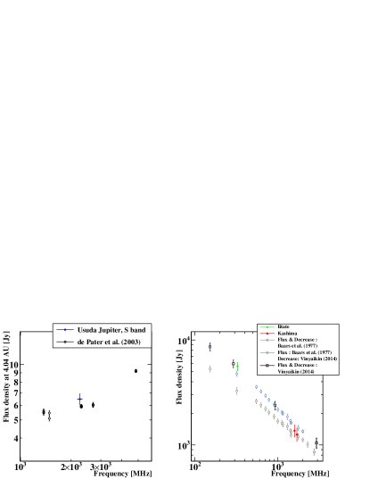
Figure 18.— Flux densities of Jupiter (left) and Cas A (right). Our data and previous observations (de Pater et al., 2003; Baars et al., 1977; Vinyaikin, 2014) are plotted. As for Jupiter, our data is normalized to the flux at the distance of 4.04 au for comparison with the other data. Taking into account that the fluxes of Cas A show secular decrease with a frequency-dependent rate, we plot three cases with different combinations of the literal flux density and decrease rate of Baars et al. (1977) and Vinyaikin (2014).

We also compare the period mean flux density of the Crab pulse (e.g. Maron et al., 2000) with previous studies in each frequency band. In Figure 19, our results agree with previous studies (Sieber, 1973; Lorimer et al., 1995; Moffett & Hankins, 1996). The significant pulse signals were not detected at C and X bands, which may be due to the effects of the interstellar scintillation.

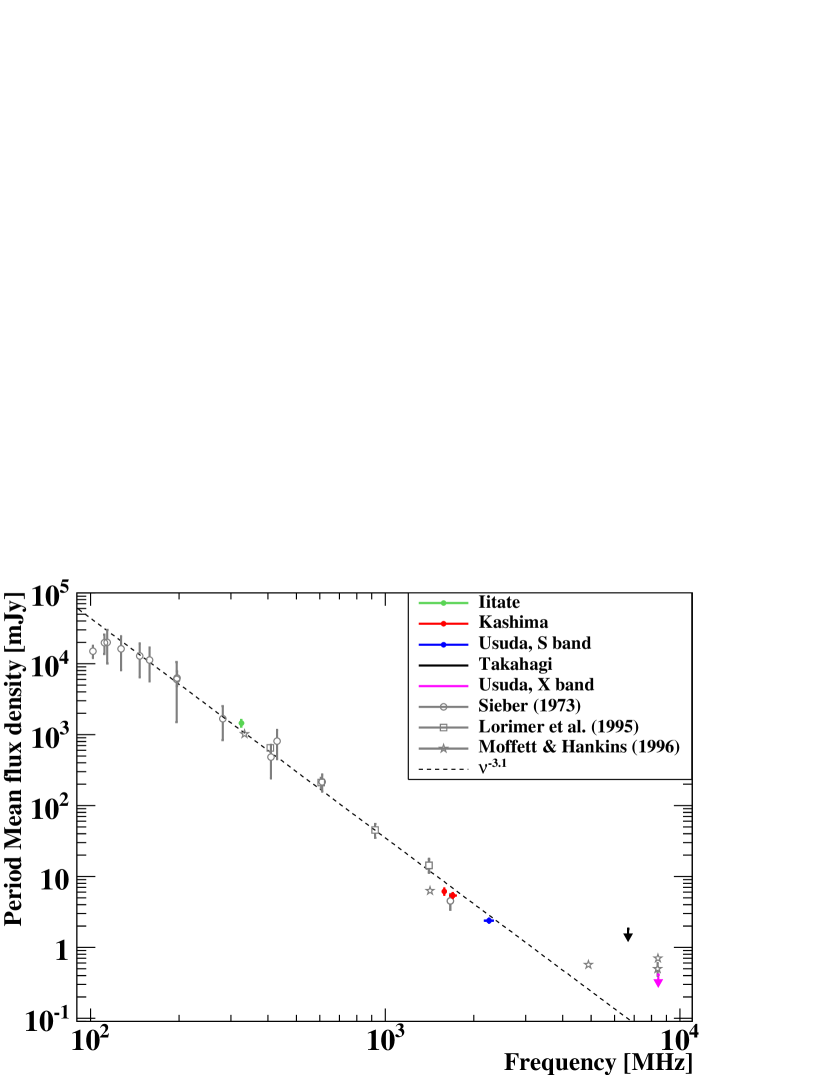
Figure 19.— Period mean flux density of the Crab pulse. Our data and previous observations (Sieber, 1973; Lorimer et al., 1995; Moffett & Hankins, 1996) are plotted. The dotted line is a reference one showing $\propto\nu^{-3.1}$ (Lorimer et al., 1995). For the C and X bands, our observation yields just upper-limit values.

Appendix B Time Interval for Fluence Estimate

As long as a GRP is selected in a certain band with the method described in Section 2.1, the fluences or their upper-limits are estimated for all the bands. To obtain those values, we need to set a time interval for the integral. If we adopt a time interval that is too long compared to the actual duration of a GRP, an excessively large error in $F$ will be obtained. Each GRP in each observational band shows a different duration. While the typical duration in LL band is a few $\mu$s, several GRPs with a duration of $\sim 20\ \mu$s were also observed. Therefore, we determine the time interval for each GRP individually. A characteristic difficulty in our analysis arises from the very different duration timescales in the P band and the other L/S bands. According to the phase distributions of the GRP signals detected at both the LL and P bands, we empirically established the method to determine the interval as follows. According to the method described in Section 2.1, we search for GRPs at P–S bands. Taking into account the different timescales in P and the other bands, we divide the GRP samples into two cases: (1) there are signals above the GRP selection thresholds in the data of at least one of LL, LH, and S bands. (2) there are signals above the GRP selection thresholds only in the P band data.

B.1. GRPs Selected at LL/LH/S Bands

In the three bands, LL, LH, or S, we occasionally found a misaligned GRP in different bands or a GRP that has a long quiescent period between two pulses (see e.g. Figure 2). Therefore, we use all the light curves in the three bands to determine the time interval, which is commonly adopted for all the three bands. The fluences are calculated based on the 1$\mu$s time-bin data. From the 10$\mu$s time-bin light curves, we first determine a tentative time interval as follows. When a GRP is selected in some of the three bands, at least one time bin of S/N$>6$ exists. In the three light curves, we search for a single time bin of S/N$>6$ or multiple successive time bins of S/N$>4$. The time interval $(t_{1},t_{2})$ is defined as the minimal interval that contains all the above high S/N time bins. Then, we generate the time series of the data with 1$\mu$s time-bin for all the three bands for the time interval $(t_{1}-10\mu\mbox{s},t_{2}+10\mu\mbox{s})$. From those three data sets, we define the bin numbers at which the first and last S/N$>3$ signal appears as $i_{\rm s}$ and $i_{\rm e}$, respectively. Taking into account the time accuracy between the instruments ($\sim 1\ \mu$s), we integrate the data over time bins from $i_{\rm s}-1$ to $i_{\rm e}+1$ to estimate the fluences or their upper limits for LL, LH, and S bands.

For the P band, the time series of the data is generated with 500$\mu$s time bin. Since the GRP duration in L/S band is short, the bin number $i_{\rm m}$ corresponding to the L/S GRP time is uniquely determined. When the highest S/N in the interval $(i_{\rm m}-1,i_{\rm m}+2)$ is below four, we set an upper limit of the fluence using the same interval. This time interval is based on the fact that 95% of P-band GRPs have a duration shorter than $2000\ \mu$s. Including the case that a P band GRP is selected, when the highest S/N is above four, we set the highest bin as the starting point, and extend the interval back and forward as long as the successive time bin has S/N$>2$. This is because a strong P-band GRP tends to show a long tail in its light curve. We integrate over this time interval of S/N$>2$ and estimate the fluence.

B.2. GRPs Selected at Only P Band

When a GRP is selected at only P band, the method to determine the time interval for the P band is the same as in the previous case. In this case, the highest signal in the other bands is below the selection threshold. In the duration of a P-band GRP, there are $1000$ or more time bins in the LL, LH, and S band light curves of $\Delta t=1\ \mu$s. In those large data sets, several time bins of S/N$\sim 3$ or 4 may appear as the statistical fluctuation. Therefore, it is dangerous to search for a weak GRP signal in such a long timescale. In this case, we set upper limits of the fluences at LL/LH/S bands. From all the three light curves of $\Delta t=10\ \mu$s, we search for the highest S/N time bin. Centering this time bin, we integrate the data over 30$\mu$s to obtain the upper limits.

Appendix C Error Estimate for LH and S Bands

In our analysis, we synthesized the flux densities for L6–L8 and S1–S5 channels into LH and S bands, respectively. While the statistical errors in the synthesized flux are estimated with the standard manner taking into account the overlaps of the frequency intervals, the systematic error is evaluated by a sum of the systematic errors of the individual channels. The obtained errors become significantly small owing to the channel synthesis as shown in the central panel of Figure 20. Hereafter, this standard method is called “method A”, which is the method adopted in the analysis in the main text.

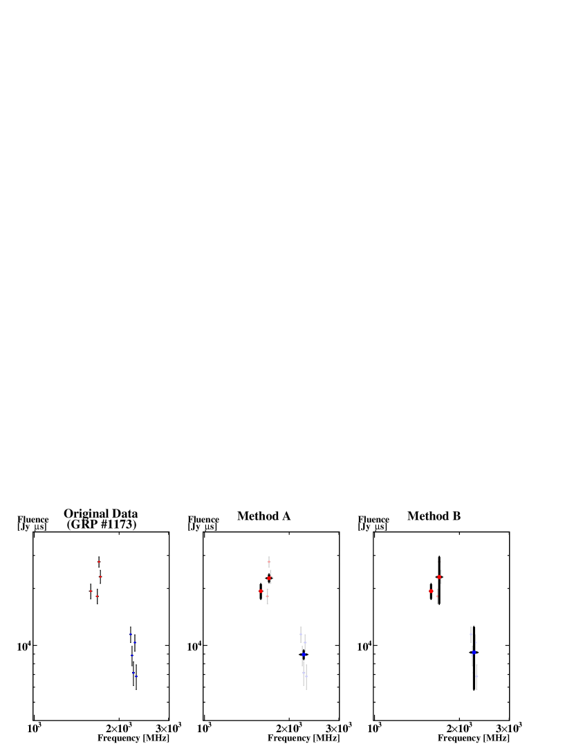
Figure 20.— Error estimates for the fluences at LH and S bands. Left: original data points of the four channels in the L band (red), and five channels in the S band (blue) for GRP #1173. Middle: synthesized data points and errors at LH and S bands with the method A. Right: the same as the middle panel but for the conservative error estimate with the method B.

The obtained fluences for the individual channels frequently show significant variations within their narrow frequency range as seen in the left panel of Figure 20. As Karuppusamy et al. (2010) claimed, the fluence fluctuation in the narrow bands may be intrinsic property in the GRP spectra similarly to the band spectral structure seen in Hankins & Eilek (2007). Although the modulation due to the diffractive interstellar scintillation may be negligible at the channels in the L and S bands as discussed in Section 3, the fluctuation may be the result of the unknown effects of the interstellar scintillation. In order to take into account this uncertainty, we attempt another conservative method for the error estimate of the synthesized fluences, “method B”. In this method, the actual fluence is assumed to be between the highest and the lowest values in the fluences for the channels in each band. The upper and lower limits in the fluence $F_{\rm max}$ and $F_{\rm min}$ are defined as follows,

$$F_{\rm max}\equiv\max(F_{\rm{ch}}+\sigma_{\rm{ch}}),\quad F_{\rm min}\equiv\min(F_{\rm{ch}}-\sigma_{\rm{ch}}),$$

where $F_{\rm{ch}}$ and $\sigma_{\rm{ch}}$ are the fluence and its $1\sigma$ error, respectively, at channel $\rm{ch}=\rm{L6,L7,L8}$ or S1, S2, S3, S4, S5. In the method B, the representative fluence $F$ and its $1\sigma$ error $\sigma_{\rm tot}$ are assumed as

$$F = \frac{F_{\rm max}+F_{\rm min}}{2},$$ (C2)

$$\sigma_{\rm tot} = F-F_{\rm min}=F_{\rm max}-F.$$ (C3)

As shown in the right panel of Figure 20, the method B leads to larger errors. When there is a channel with a fluence below $3\sigma_{\rm{ch}}$, we set an upper-limit $F_{\rm max}$ on the fluence. In this conservative method, even if an S/N value for the synthesized channel is above the selection threshold, there are cases in which just the upper limit is set on the synthesized fluence. Therefore, some fraction of GRPs detected with the method A are judged as non-detection. The sample number in the method B becomes slightly smaller than that in the method A (compare Tables 4 and 7).

When we use the data generated with the method B in the spectral analysis, 95.6% of MPGRPs and 97.0% of IPGRPs are judged to be consistent with SPLs at a significance level of 5% (see Table 7).

Table 7The same table as Table 4, but with the conservative error estimate, method B.

		SPL Hypothesis (MPGRP)			SPL Hypothesis (IPGRP)
Detection Y/N	Groupa	Consistent	Inconsistent		Consistent	Inconsistent
(P, LL, LH, S band)		($\hat{\chi}_{\mbox{min}}^{2}<5.99$)	($\hat{\chi}_{\mbox{min}}^{2}>5.99$)		($\hat{\chi}_{\mbox{min}}^{2}<5.99$)	($\hat{\chi}_{\mbox{min}}^{2}>5.99$)
(Y, Y, Y, Y)	I	163	20		26	2
(Y, Y, Y, N)	I	61	3		12	0
(Y, N, N, Y)	I	3	1		0	0
(Y, Y, N, Y)	I	9	0		0	0
(Y, N, Y, Y)	I	1	0		0	0
(Y, Y, N, N)	I	15	0		6	0
(Y, N, Y, N)	I	3	0		1	0
(N, Y, Y, Y)	II	944	59 ($\alpha>2$ : 1)		60	0
(N, Y, N, Y)	II	165	1		10	0
(N, N, Y, Y)	II	39	2		1	0
(N, Y, Y, N)	$\cdots$	408	25		28	2
(N, N, N, Y)	$\cdots$	146	1 ($\alpha>2$ : 1)		4	0
(N, Y, N, N)	$\cdots$	278	15		23	2
(N, N, Y, N)	$\cdots$	79	2		2	0
(Y, N, N, N)	III	480	1 ($\alpha<-5$ : 1)		53	1 ($\alpha<-5$ : 1)
Total		2794	130		226	7
			($\alpha>2$ : 2, $\alpha<-5$ : 1)			($\alpha>2$ : 0, $\alpha<-5$ : 1)

a: We categorize the GRPs into three groups, from I to III. See Section 3.1.

Appendix D Monte Carlo Simulations for the apparent correlations

Some correlations between the fluences and spectral indices are found in our analysis. In order to probe the intrinsic distributions of the fluences and indices, we simulate multi-frequency observations of SPL GRPs with the Monte Carlo method, assuming that an intrinsic correlation between the fluence and hardness is absent. However, we should notice that for given fluence at L/S band, a smaller spectral index implies a larger energy release at the P band, where most of the energy is released. Namely, the uncorrelation between the fluences at L/S band and $\alpha$ is equivalent to the assumption of an anti-correlation between the total energy release and hardness. As will be shown, this assumption seems most likely to reproduce the observed correlations.

In Figure 21, we show the scatter plot of Group (I) MPGRPs detected at the LL band, obtained with the method B (see Appendix C), for the fluence at the LL band ($F_{\rm LL}$) and the spectral index ($\alpha$). While the sample number is larger than that with method A in Section 3.4, the similar correlation is seen. To reproduce this correlation, we generate pseudo GRP samples whose fluence distribution at the LL band follows the power law with index -2.98 as observed (see Table 3) above $1260$Jy $\mu$s. The suppression in the lower fluence region (“roll-over” feature) seen in the distributions shown in Figure 4 may be due to the decline of the detection efficiency. The detection efficiency in the lower fluence region for each band is determined to reproduce the roll-over shape. For each pseudo GRP, we obtain $\alpha$ following a distribution assumed in advance, independently of $F_{\rm LL}$. The fluence at other bands is calculated with the obtained $F_{\rm LL}$ and $\alpha$. We judge the detection of the pseudo GRPs taking into account the detection efficiency at each frequency band, and then categorize the GRPs into the groups described in Section 3.1. The GRP sample generation continues until the number of GRPs detected at both P and LL bands reaches 271, which is the number of GRPs detected at both the P and LL bands in our observation samples. Since 248 GRPs (samples in Figure 21) are judged to be consistent with a SPL, we randomly extract 248 GRPs from the 271 pseudo samples. We perform such trials $10^{4}$ times for a certain distribution of $\alpha$.

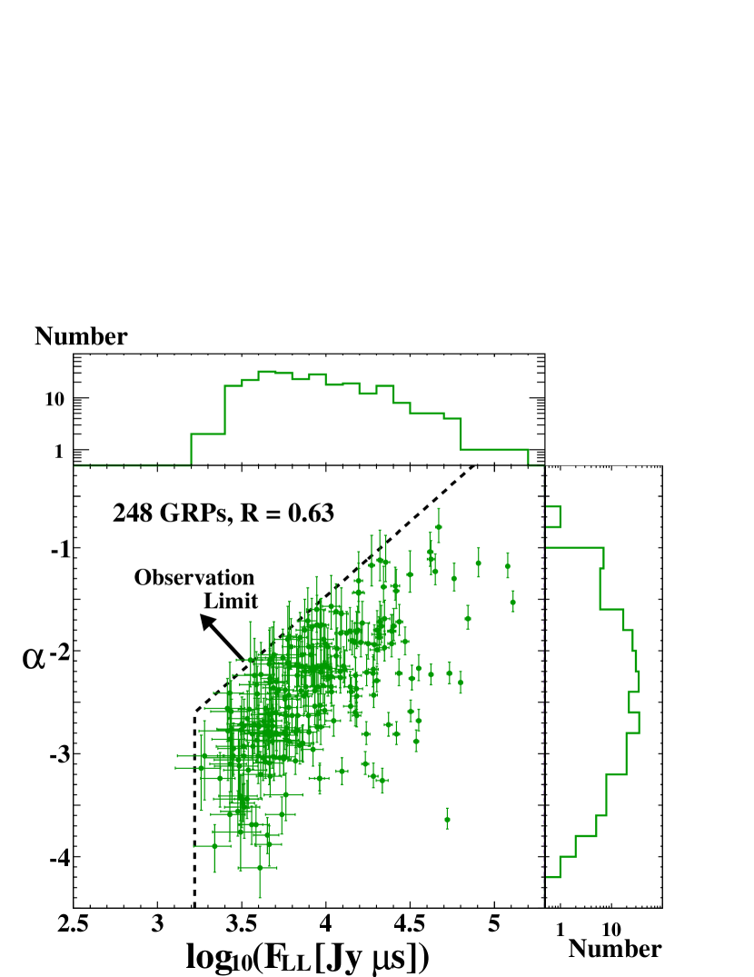
Figure 21.— Scatter plot of $F_{\rm LL}$ and $\alpha$ for the Group (I) MPGRPs selected with the method B.

First, we test a uniform distribution from $\alpha=-4.0$ to $0.0$, and a Gaussian distribution with the mean value of $\bar{\alpha}=-3.0$, which is close to that for the normal pulse (e.g. Moffett & Hankins, 1999), and the standard deviation $\sigma_{\alpha}=1.0$. For those models, examples of the scatter plots obtained from one of the trials are shown in Figure 22. Apparently, the distributions seem different from the observed one. We calculate the Spearman rank correlation coefficient $R_{\rm LL}$ for those 248 pseudo samples in each trial, but none of the trials reaches $0.63$, the value for the actual Group (I) GRPs (see Figure 24). The uniform distribution and $\bar{\alpha}=-3.0$ are excluded.

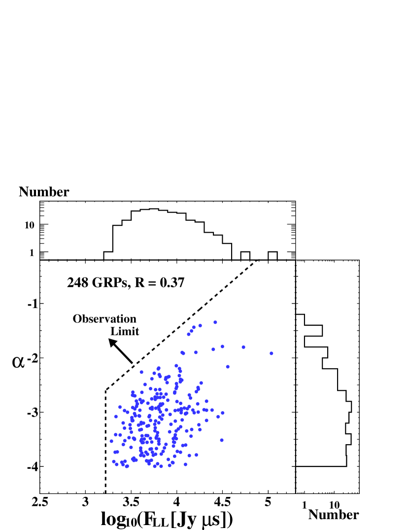
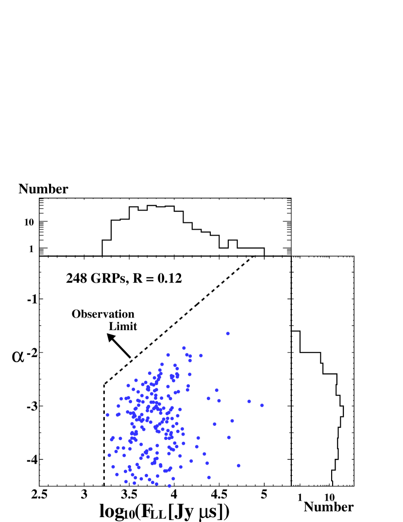
Figure 22.— Scatter plots of $F_{\rm LL}$ and $\alpha$ for pseudo samples with a uniform $\alpha$ distribution from $-4.0$ to $0.0$ (left), and a Gaussian one with $(\bar{\alpha},\sigma_{\alpha})=(-3.0,1.0)$ (right).

However, if the typical index is harder than that for the normal pulse, only a small fraction of dim GRPs at the LL band is soft enough to be detected at the P band. Here, we show the results for the Gaussian distributions with $(\bar{\alpha},\sigma_{\alpha})=(-1.0,0.9)$ as an example. The distributions in the LL and P bands for those models, as shown in Figure 23, are similar to Figures 21 and 11, respectively.

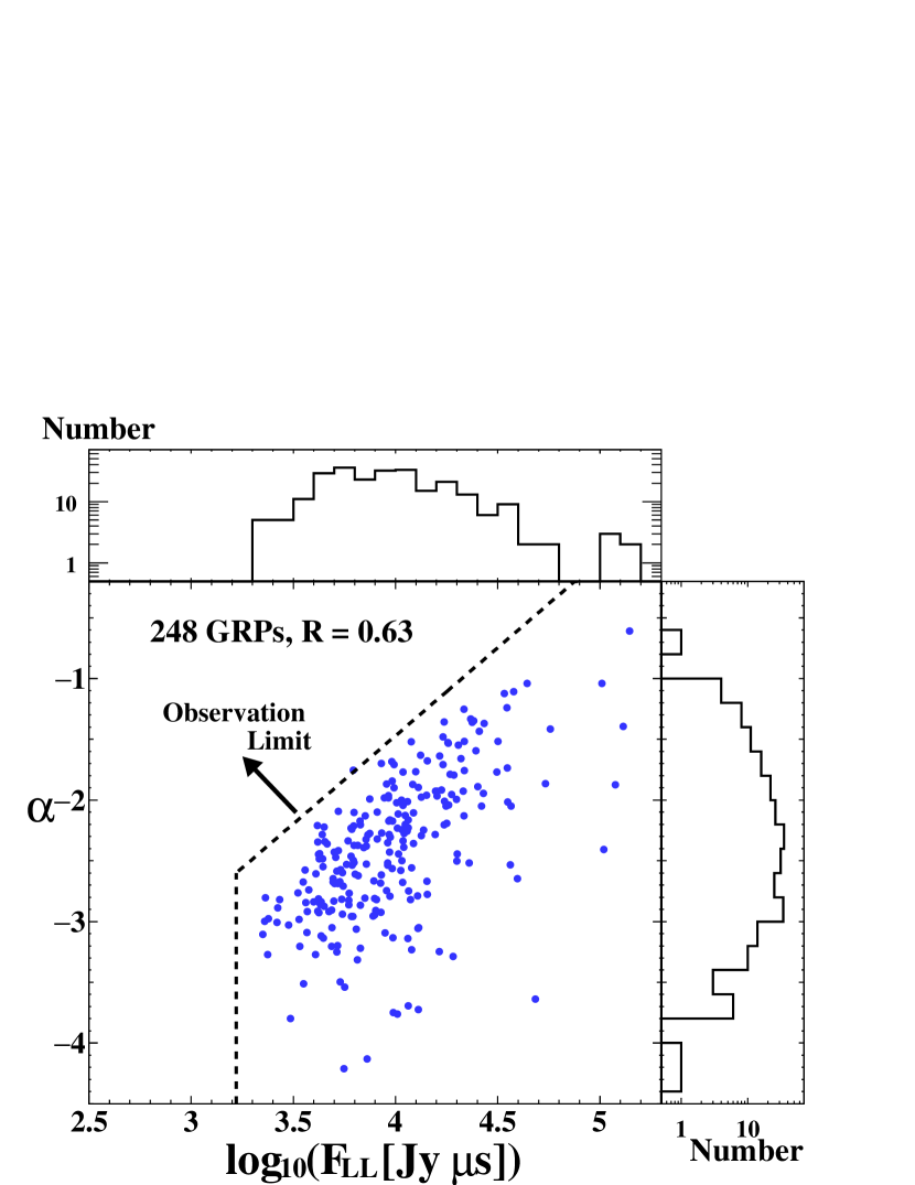
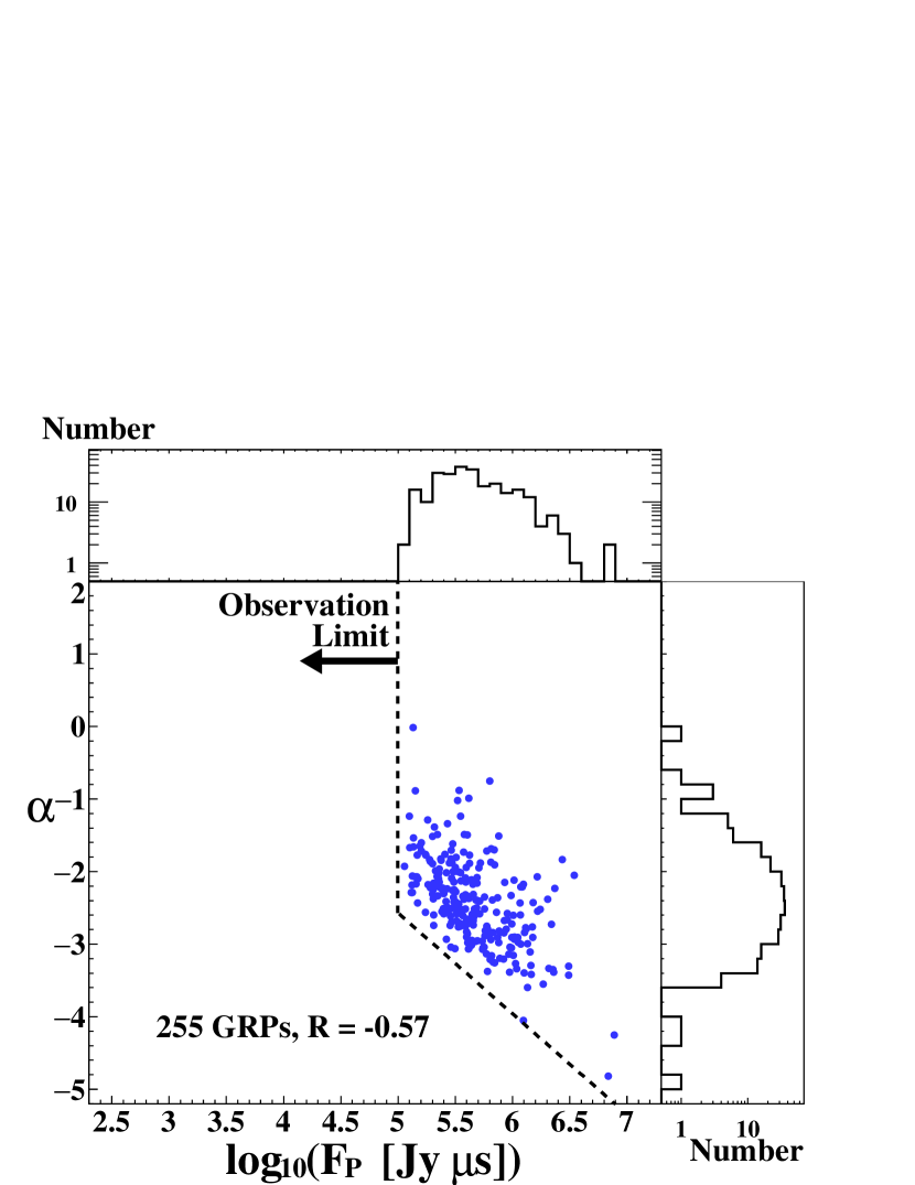
Figure 23.— Scatter plots for pseudo samples with a Gaussian distribution for $\alpha$ with $(\bar{\alpha},\sigma_{\alpha})=(-1.0,0.9)$ in the LL (left) and P (right) bands.

Actually, in this model, the distributions of the Spearman rank correlation coefficient is consistent with the obtained values from our observation as shown in Figure 24. Moreover, the number of GRPs detected at the P band, the number of Group (III) GRPs, and the power-law index of the fluence distribution at the P band in this model roughly agree with our observation (see Figure 25). This model overpredicts the number of the GRPs detected at only the S band. Many hard GRPs ($\alpha>0.0$) contribute to those S-band GRPs. This may indicate that the $\alpha$ distribution is asymmetric. When we artificially suppress GRPs with $\alpha\gtrsim 0.0$ compared to the exact Gaussian distribution, the correlations are maintained, and the number of GRPs detected at only S band becomes consistent with our real samples. The actual distribution may have a sharp peak around $-1$ and one-sided long tail at $\alpha<-1$.

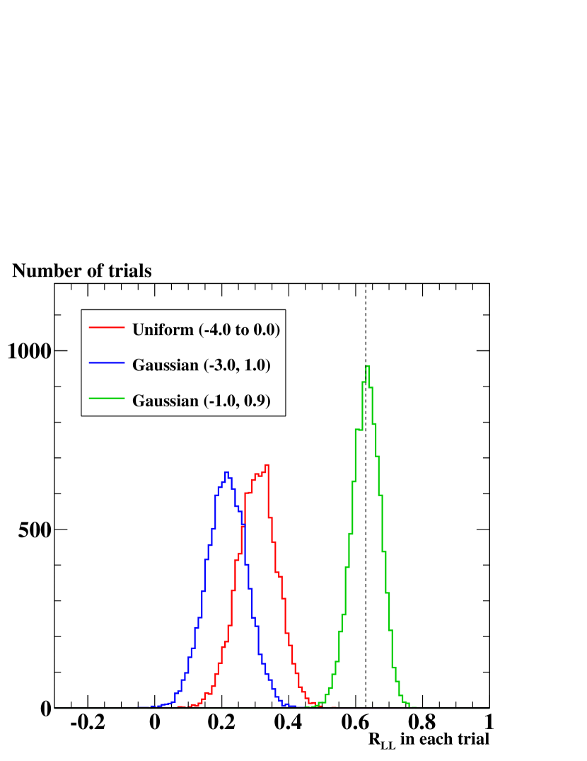
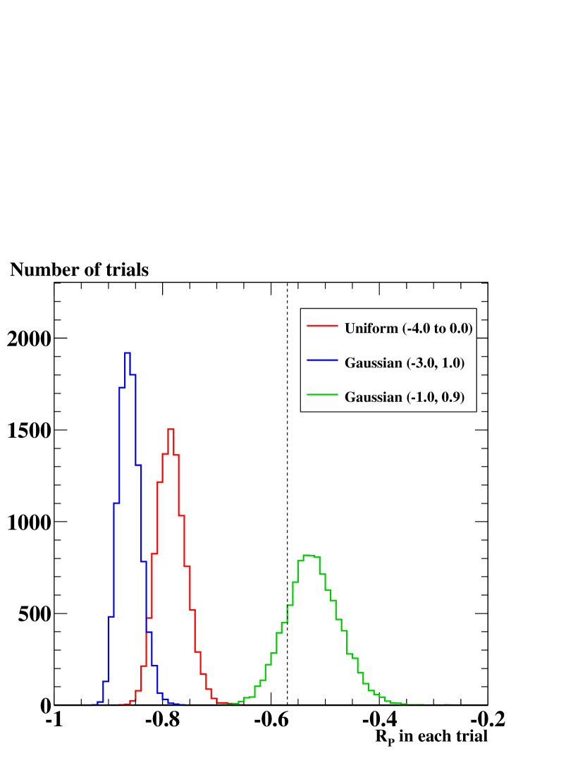
Figure 24.— Distributions of the Spearman rank correlation coefficient in the LL (left) and P (right) bands for the pseudo samples of the different $\alpha$ distributions. In each model, we test $10^{4}$ trials. The dashed lines represent the values obtained from the real data with the method B.

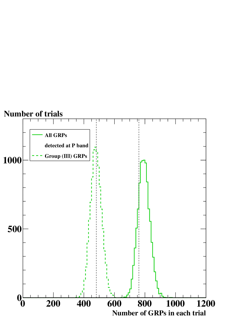
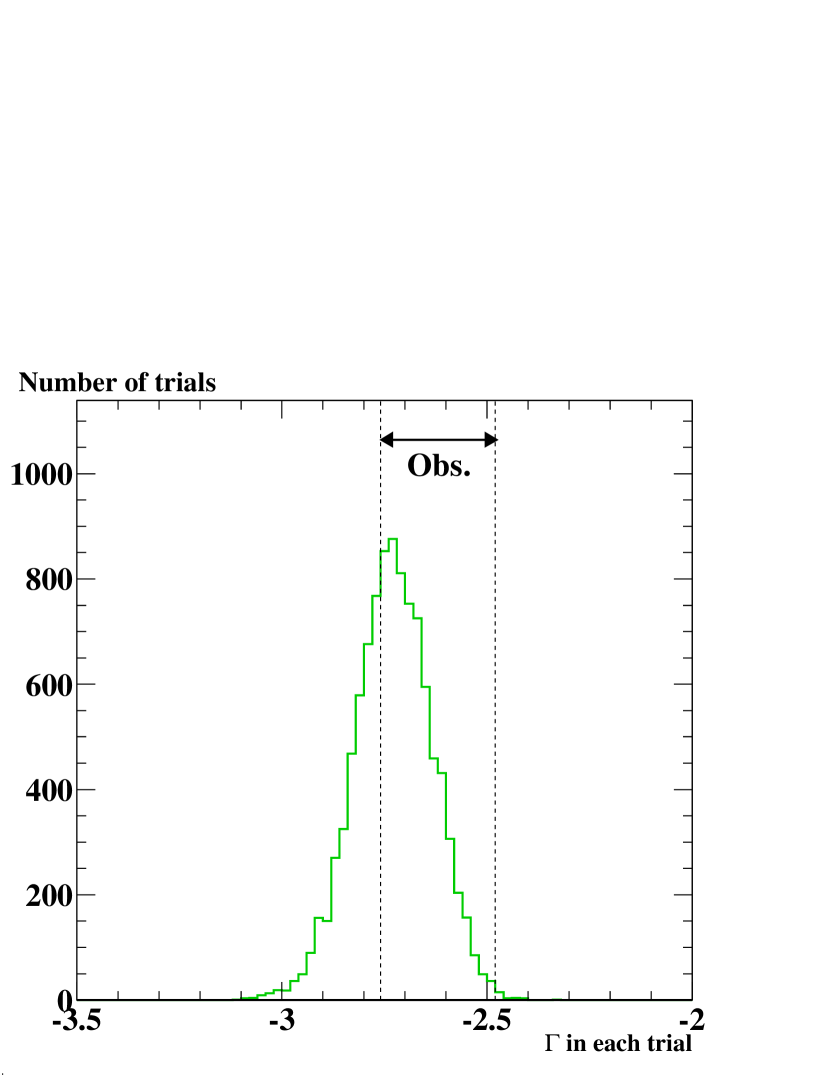
Figure 25.— Distributions of the number of GRPs detected at P band, the number of Group (III) GRPs (left), and the power-law index in the fluence distribution at P band (right) for the pseudo samples of the Gaussian $\alpha$ distribution of $(\bar{\alpha},\sigma_{\alpha})=(-1.0,0.9)$, based on $10^{4}$ trials. The dashed lines represent the values obtained from the real data.

References

- Amato et al. (2000) Amato, E., Salvati, M., Bandiera, R., Pacini, F., & Woltjer, L. 2000, A&A, 359, 1107
- Aoki et al. (2014) Aoki, T., Tanaka, T., Niinuma, K., et al. 2014, ApJ, 781, 10
- Argyle & Gower (1972) Argyle, E., & Gower, J. F. R. 1972, ApJ, 175, L89
- Avni et al. (1980) Avni, Y., Soltan, A., Tananbaum, H., & Zamorani, G. 1980, ApJ, 238, 800
- Baars et al. (1977) Baars, J. W. M., Genzel, R., Pauliny-Toth, I. I. K., & Witzel, A. 1977, A&A, 61, 99
- Bandura et al. (2014) Bandura, K., Addison, G., Amiri, M., et al. 2014, Proc. SPIE, 9145, 22
- Bera et al. (2016) Bera, A., Bhattacharyya, S., Bharadwaj, S., Bhat, N. D. R., & Chengalur, J. N. 2016, MNRAS, 457, 2530
- Bhat et al. (2008) Bhat, N. D. R., Tingay, S. J., & Knight, H. S. 2008, ApJ, 676, 1200
- Bietenholz et al. (2015) Bietenholz, M. F., Yuan, Y., Buehler, R. Lobanov, A. P. & Blandford, R. 2015, MNRAS, 446, 205
- Bilous et al. (2011) Bilous, A. V., Kondratiev, V. I., McLaughlin, M. A., et al. 2011, ApJ, 728, 110
- Bilous et al. (2015) Bilous, A. V., Pennucci, T. T., Demorest, P., & Ransom, S. M. 2015, ApJ, 803, 83
- Burke-Spolaor et al. (2012) Burke-Spolaor, S., Johnston, S., Bailes, M., et al. 2012, MNRAS, 423, 1351
- Burke-Spolaor et al. (2016) Burke-Spolaor, S., Trott, C. M., Brisken, W. F., et al. 2016, ApJ, 826, 223
- Cheng & Ruderman (1980) Cheng, A. F., & Ruderman, M. A., 1980, ApJ, 235, 576
- Connor et al. (2016) Connor, L., Sievers, J., & Pen, U. 2016, MNRAS, 458, L19
- Cordes et al. (2004) Cordes, J. M., Bhat, N. D. R., Hankins, T. H., McLaughlin, M. A., & Kern, J. 2004, ApJ, 612, 375
- Cordes & Wasserman (2016) Cordes, J. M., & Wasserman, Ira 2016, MNRAS, 457, 232
- Cronyn (1970) Cronyn, W. M., 1970, Science, 168, 1453
- de Pater et al. (2003) de Pater, I., Butler, B. J., Green, D. A., et al. 2003, Icar, 163, 434
- Dicke (1946) Dicke, R. H. 1946, RScI, 17, 268
- Ellingson et al. (2013) Ellingson, S. W., Clarke, T. E., Craig, J., et al. 2013, ApJ, 768, 136
- Hankins & Rickett (1975) Hankins, T. H., & Rickett, B. J. 1975, in Methods in Computational Physics, Vol. 14: Radio Astronomy (New York: Academic), 55
- Hankins et al. (2003) Hankins, T. H., Kern, J. S., Weatherall, J. C., & Eilek, J. A. 2003, Nature, 422, 141
- Hankins & Eilek (2007) Hankins, T. H., & Eilek, J. A. 2007, ApJ, 670, 693
- Hankins et al. (2015) Hankins, T. H., Jones, G., & Eilek, J. A. 2015, ApJ, 802, 130
- Hobbs et al. (2006) Hobbs, G. B., Edwards, R. T., & Manchester, R. N. 2006, MNRAS, 369, 655
- Jessner et al. (2005) Jessner, A., Słowikowska, A., Klein, B., et al. 2005, AdSpR, 35, 1166
- Johnston & Romani (2003) Johnston, S. & Romani, R. W. 2003, ApJ, 590, L95
- Karuppusamy et al. (2010) Karuppusamy, R., Stappers, B. W., & van Straten, W. 2010, A&A, 515, A36
- Kashiyama et al. (2013) Kashiyama, K., Ioka, K., & Mészáros, P. 2013, ApJ, 776, L39
- Kazantsev & Potapov (2015) Kazantsev, A. N., & Potapov, V. A. 2015, A Tsir, 1628, 1
- Keane et al. (2012) Keane, E. F., Stappers, B. W., Kramer, M., & Lyne, A. G. 2012, MNRAS, 425, L71
- Keane et al. (2016) Keane, E. F., Johnston, S., Bhandari, S., et al. 2016, Nature, 530, 453
- Kisaka et al. (2016) Kisaka, S., Asano, K., & Terasawa, T. 2016, ApJ, 829, 12
- Kondo et al. (2003) Kondo, T., Koyama, Y., Nakajima, J., Sekido, M., & Osaki, H. 2003, in ASP Conf. Ser., 306 “New Technologies in VLBI”, ed. Y. C. Minh (San Francisco: ASP), 205
- Kramer et al. (2003) Kramer, M., Karastergiou, A., Gupta, Y., et al. 2003, A&A, 407, 655
- Kuzmin et al. (2008) Kuzmin, A., Losovsky, B. Ya. , Jordan, C. A., & Smith, F. G. 2008, A&A, 483, 13
- Lampton et al. (1976) Lampton, M., Margon, B., & Bowyer, S. 1976, ApJ, 208, 177
- Lorimer et al. (1995) Lorimer, D. R., Yates, J. A., Lyne, A. G., & Gould, D. M. 1995, MNRAS, 273, 411
- Lorimer & Kramer (2004) Lorimer, D. R., & Kramer, M. 2004, Handbook of Pulsar Astronomy (Cambridge: Cambridge Univ. Press)
- Lorimer et al. (2007) Lorimer, D. R., Bailes, M., McLaughlin, M. A., Narkevic, D. J., & Crawford, F. 2007, Sci, 318, 777
- Lu & Kumar (2016) Lu, Y., & Kumar, P. 2016 arXiv:1605.04605
- Lyne et al. (1993) Lyne, A. G., Pritchard, R. S. & Graham-Smith, F. 1993. MNRAS, 265, 1003
- Lyutikov (2007) Lyutikov, M. 2007, MNRAS, 381, 1190
- Macías-Perez et al. (2010) Macías-Pérez, J. F., Mayet, F., Aumont, J., & Désert, F.-X. 2010, ApJ, 711, 417
- Majid et al. (2011) Majid, W. A., Naudet, C. J., Lowe, S. T., & Kuiper, T. B. H. 2011, ApJ, 741, 53
- Maron et al. (2000) Maron, O., Kijak, J., Kramer, M., & Wielebinski, R. 2000, A&AS, 147, 195
- Mickaliger et al. (2012) Mickaliger, M. B., Mclaughlin, M. A., Lorimer, D. R., et al. 2012, ApJ, 760, 64
- Misawa et al. (2003) Misawa, H., Kudo, R., Tsuchiya, F., Morioka, A., & Kondo, T. 2003, in Proceedings of the 3rd CRL TDC Symposium, ed. T. Kondo & Y. Koyama (CRL, Koganei), 57
- Moffett & Hankins (1996) Moffett, D. A., & Hankins, T. H. 1996, ApJ, 468, 779
- Moffett & Hankins (1999) Moffett, D. A., & Hankins, T. H. 1999, ApJ, 522, 1046
- Oronsaye et al. (2015) Oronsaye, S. I., Ord, S. M., Bhat, N. D. R., et al. 2015, ApJ, 809, 51
- Petrova (2004) Petrova, S. A. 2004, A&A, 424, 227
- Popov et al. (2008) Popov, M. V., Soglasnov, V. I., Kondratiev, A. V., et al. 2008, ARep, 52, 900
- Popov et al. (2009) Popov, M., Soglasnov, V., Kondratiev, V., et al. 2009, PASJ, 61, 1197
- Press et al. (1992) Press, W. H., Teukolsky, S. A., Vetterling, W. T., & Flannery, B. P. 1992, in Numerical Recipes in C. The Art of Scientific Computing, ed. W. H. Press, S. A. Teukolsky, W. T. Vetterling, & B. P. Flannery (2nd ed.; Cambridge: Cambridge Univ. Press)
- Ravi et al. (2015) Ravi, V., Shannon, R. M., & Jameson, A. 2015, ApJ, 799, L5
- Rickett & Lyne (1990) Rickett, B. J., & Lyne A. G. 1990, MNRAS, 244, 68
- Rosenberg (1970) Rosenberg, I. 1970, MNRAS, 147, 215
- Sallmen et al. (1999) Sallmen, S., Backer, D. C., Hankins, T. H., et al. 1999, ApJ, 517, 460
- Sawicki (2012) Sawicki, M. 2012, PASP, 124, 1208
- Scholz et al. (2016) Scholz, P., Spitler, L. G., Hessels, J. W. T., et al. 2016, arXiv:1603.08880
- Sieber (1973) Sieber, W. 1973, A&AS, 28, 237
- Soglasnov et al. (2004) Soglasnov, V. A., Popov, M. V., Bartel, N., et al. 2004, ApJ, 616, 439
- Spitler et al. (2016) Spitler, L. G., Scholz, P., Hessels, J. W. T., et al. 2016, Nature, 531, 202
- Tanaka et al. (2015) Tanaka, S. J., Asano, K., & Terasawa, T. 2015, PTEP, 2015, 073E01
- Takefuji et al. (2010) Takefuji, K., Takeuchi, H., Tsutsumi, M., & Koyama, Y. 2010, in IVS 2010 General Meeting Proceedings, ed. D. Behrend, & K. D. Baver (IVS Coordinating Center NASA Goddard Space Flight Center Code 698.2: Greenbelt, MD), 378
- Takefuji et al. (2016) Takefuji, K., Terasawa, T., Kondo, T., et al. 2016, PASP, 128, 084502
- Thornton et al. (2013) Thornton, D., Stappers, B., Bailes, M., et al., 2013, Science, 341, 53
- Timokhin & Arons (2013) Timokhin, A. N., & Arons, J. 2013, MNRAS, 429, 20
- Totani (2013) Totani, T. 2013, PASJ, 65, L12
- Tsai et al. (2015) Tsai, -Wei, Jr, Simonetti, J. H., Akukwe, B., et al. 2015, AJ, 149, 65
- Tsuchiya et al. (2010) Tsuchiya, F., Misawa, H., Imai, K., Morioka, A., & Kondo, T. 2010, AdG, 19, 601
- Vinyaikin (2014) Vinyaikin, E. N., 2014, ARep, 58, 626
- Wang & Yu (2016) Wang, F. Y., & Yu, H. 2016, arXiv:1604.08676
- Wilson et al. (2013) Wilson, T. L., Rohlfs, K., & Hüttemeister, S. 2013, Tools of Radio Astronomy (Berlin: Springer)
- Yonekura et al. (2016) Yonekura, Y., Saito, Y., Sugiyama, K., et al. 2016, PASJ, 68, 74