Proximal methods for stationary Mean Field Games with local couplings

Abstract

We address the numerical approximation of Mean Field Games with local couplings. For power-like Hamiltonians, we consider both the stationary system introduced in [51, 53] and also a similar system involving density constraints in order to model hard congestion effects [65, 57]. For finite difference discretizations of the Mean Field Game system as in [3], we follow a variational approach. We prove that the aforementioned schemes can be obtained as the optimality system of suitably defined optimization problems. In order to prove the existence of solutions of the scheme with a variational argument, the monotonicity of the coupling term is not used, which allow us to recover general existence results proved in [3]. Next, assuming next that the coupling term is monotone, the variational problem is cast as a convex optimization problem for which we study and compare several proximal type methods. These algorithms have several interesting features, such as global convergence and stability with respect to the viscosity parameter, which can eventually be zero. We assess the performance of the methods via numerical experiments.

1 Introduction

Mean Field Games (MFG) have been recently introduced by J.-M. Lasry and P.-L. Lions [51, 52, 53] and by Huang, Caines, and Malhamé [49] in order to model the behavior of some differential games when the number of players tends to infinity. For finite-horizon games, and under suitable assumptions such as the absence of a common noise affecting simultaneously all agents, the description of the limiting behaviour collapses into two coupled deterministic partial differential equations (PDEs). The first one is a Hamilton-Jacobi-Bellman (HJB) equation with a terminal condition, characterizing the value function $v$ of an optimal control problem solved by typical small player and whose cost function depends on the distribution $m$ of the other players at each time. The second one is a Fokker-Planck (FP) equation, describing, at the Nash equilibrium, the evolution of the initial distribution $m_{0}$ of the agents. In the ergodic case, the resulting system is stationary and its solution is the limit of a rescaled solution of a finite-horizon MFG system when the horizon tends to infinity (see [27, 28, 25] and also [44] for similar results in the context of discrete MFG).

In order to introduce the system we study, let $\mathbb{T}^{n}$ be the $n$-dimensional torus and $f:\mathbb{T}^{n}\times[0,+\infty[\to\mathbb{R}$ be a continuous function. Given $\nu\geq 0$ and a function $H:\mathbb{T}^{n}\times\mathbb{R}^{n}\mapsto\mathbb{R}$, such that for all $x\in\mathbb{T}^{n}$ the function $H(x,\cdot):p\mapsto H(x,p)$ is convex and differentiable, we consider the following stationary MFG problem: find two functions $u$, $m$ and $\lambda\in\mathbb{R}$ such that

$$\begin{array}[]{rcl}-\nu\Delta u+H(x,\nabla u)-\lambda&=&f(x,m(x))\hskip 5.69046pt\mbox{in ${\mathbb{T}}^{n}$},\\[4.0pt] -\nu\Delta m-\mbox{div}\left(\partial_{p}H(x,\nabla u)m\right)&=&0\hskip 5.69046pt\mbox{in ${\mathbb{T}}^{n}$},\\[5.0pt] m\geq 0,\;\;\;\int_{{\mathbb{T}}^{n}}m(x){\rm d}x=1,&&\;\int_{{\mathbb{T}}^{n}}u(x){\rm d}x=0.\end{array}$$ (1.1)

When $\nu>0$, well-posedness of system (1.1) has been studied in several articles, starting with the works by J.-M. Lasry and P.-L. Lions [51, 53], followed by [45, 46, 33, 43, 7, 61] in the case of smooth solutions and [33, 11, 39, 34] in the case of weak solutions.

Let us point out that in terms of the underlying game, system (1.1) involves local couplings because the right hand side of (1.1) depends on the distribution $m$ through its pointwise value (see [53]). As explained in [53], in this case system (1.1) is related to a single optimal control problem. Indeed, defining $b:\mathbb{R}\times\mathbb{R}^{n}\mapsto\mathbb{R}\cup\{+\infty\}$ and $F:{\mathbb{T}}^{n}\times\mathbb{R}\mapsto\mathbb{R}\cup\{+\infty\}$ as

$$b(x,m,w):=\left\{\begin{array}[]{ll}mH^{\ast}\left(x,-\frac{w}{m}\right)&\mbox{if }m>0,\\ 0,&\mbox{if }(m,w)=(0,0),\\ +\infty,&\mbox{otherwise}\end{array}\right.\hskip 2.84544pt\;\;F(x,m):=\left\{\begin{array}[]{ll}\int_{0}^{m}f(x,m^{\prime}){\rm d}m^{\prime},&\mbox{if }m\geq 0,\\[4.0pt] +\infty,&\mbox{otherwise,}\end{array}\right.$$ (1.2)

system (1.1) can be obtained, at least formally, as the optimality system associated to any solution $(m,w)$ of

$$\begin{array}[]{l}\inf_{(m,w)}\int_{{\mathbb{T}}^{n}}\left[b(m(x),w(x))+F(x,m(x))\right]{\rm d}x,\\[8.0pt] \mbox{subject to }\hskip 8.5359pt\begin{array}[]{rcl}-\nu\Delta m+\mbox{div}(w)&=&0\hskip 5.69046pt\mbox{in ${\mathbb{T}}^{n}$},\\[4.0pt] \int_{{\mathbb{T}}^{n}}m(x){\rm d}x&=&1.\end{array}\end{array}$$

The function $u$ in (1.1) corresponds to a Lagrange multiplier associated to the PDE constraint, $\lambda$ is a Lagrange multiplier associated to the integral constraint, and $w$ is given by $-\partial_{p}H(x,\nabla u)m$. Note that the definitions of $b$ and $F$ involve, implicitly, the non-negativity of the variable $m$.

In the presence of hard congestion effects for the agents, we consider upper bound constraints for the density $m$ (see [55, 56] for the analysis in the context of crowd motion and [65] for a proposal in the context of MFG), which we include in the following optimization problem (see [57] for a detailed study)

$$\begin{array}[]{l}\inf_{(m,w)}\int_{{\mathbb{T}}^{n}}\left[b(m(x),w(x))+F(x,m(x))\right]{\rm d}x,\\[8.0pt] \mbox{subject to }\hskip 8.5359pt\begin{array}[]{rcl}-\nu\Delta m+\mbox{div}(w)&=&0\hskip 5.69046pt\mbox{in ${\mathbb{T}}^{n}$},\\[4.0pt] \int_{{\mathbb{T}}^{n}}m(x){\rm d}x&=&1,\;\;\;\;m(x)\leq d(x)\;\;\mbox{a.e. in ${\mathbb{T}}^{n}$},\end{array}\end{array}$$

where $d\in C({\mathbb{T}}^{n})$ satisfies $d(x)>0$ for all $x\in{\mathbb{T}}^{n}$ and $\int_{{\mathbb{T}}^{n}}d(x){\rm d}x>1$. It is assumed that for all $x\in{\mathbb{T}}^{n}$

$$H^{\ast}(x,v)=\frac{1}{q}|v|^{q}\hskip 8.5359pt\mbox{for some $q>1$ and so }H(x,p)=\frac{1}{q^{\prime}}|p|^{q^{\prime}},\;\;\mbox{where }\;\frac{1}{q}+\frac{1}{q^{\prime}}=1.$$ (1.3)

The analysis in [57] is done in the case of a bounded domain ${\Omega}$, with Neumann boundary conditions for the PDE constraint and $d\equiv 1$. However, it is easy to check that the results in [57] can be adapted to our case with minor modifications. If $q>n$, it is shown that there exists at least one solution $(m,w)\in W^{1,q}({\mathbb{T}}^{n})\times L^{q}({\mathbb{T}}^{n})$ to $(P^{d})$ and there exists $(u,\lambda,p)\in W^{1,s}({\mathbb{T}}^{n})\times\mathbb{R}\times\mathcal{M}_{+}({\mathbb{T}}^{n})$, where $s\in]1,n/(n-1)[$ and $\mathcal{M}_{+}({\mathbb{T}}^{n})$ denotes the set of non-negative Radon measures on ${\mathbb{T}}^{n}$, satisfying

$$\begin{array}[]{c}-\nu\Delta u+\frac{1}{q^{\prime}}|\nabla u|^{q^{\prime}}-p-\lambda\leq f(x,m(x))\hskip 5.69046pt\mbox{in ${\mathbb{T}}^{n}$},\\[4.0pt] -\nu\Delta m-\mbox{div}\left(|\nabla u|^{\frac{2-q}{q-1}}\nabla u\,m\right)=0\hskip 5.69046pt\mbox{in ${\mathbb{T}}^{n}$},\\[4.0pt] m\geq 0,\;\;\;\int_{{\mathbb{T}}^{n}}m(x){\rm d}x=1,\;\;\;\int_{{\mathbb{T}}^{n}}u(x){\rm d}x=0,\\[6.0pt] \mbox{supp}(p)\subseteq\{m=1\},\end{array}$$ (1.4)

with the convention

$$|\nabla u|^{\frac{2-q}{q-1}}\nabla u=0\hskip 11.38092pt\mbox{if }\;q>2\hskip 11.38092pt\mbox{and }\nabla u=0.$$

The first inequality in (1.4) becomes an equality on the set $\{x\in{\mathbb{T}}^{n}\;;\;m(x)>0\}$. When $1<q\leq n$, an approximation argument shows the existence of solutions of a weak form of (1.4).

The aim of this work is to consider the numerical approximation of solutions of (1.1)-(1.4) by means of their variational formulations. For the sake of simplicity, we restrict our analysis to the 2-dimensional case, i.e., we take $n=2$ and consider Hamiltonians of the form (1.3). However, all the results in this work admit natural extensions in general dimensions and most of them are valid for more general Hamiltonians. We do not consider here the case of non-local couplings, not necessarily variational, and we refer the reader to [3, 2, 24, 29, 30, 6] for some numerical methods for this case. Inspired by [2], in the context of MFG systems related to planning problems, we follow the first discretize and then optimize strategy by considering suitable finite-difference discretizations of the PDE constraint and the cost functionals appearing in $(P)$ and $(P^{d})$. Given an uniform grid of size $h$ on the torus $\mathbb{T}^{2}$, we call $(P_{h})$ and $(P_{h}^{d})$ the chosen discrete versions of $(P)$ and $(P^{d})$, respectively. We prove the existence of at least one solution $(m^{h},w^{h})$ of the discrete variational problem $(P_{h})$, as well as the existence of Lagrange multipliers $(u^{h},\lambda^{h})$ associated to $(m^{h},w^{h})$. Similar results are obtained for $(P_{h}^{d})$, where an additional Lagrange multiplier $p^{h}$ appears because of the supplementary density constraint. We state the general optimality conditions for both problems in Theorem 2.1. If we consider problem $(P_{h})$ and we suppose that $\nu>0$, we obtain in Corollary 2.2 that $(m^{h},u^{h},\lambda^{h})$ solves the finite-difference scheme proposed by Achdou et al. in [3, 1]. We point out that, contrary to [2], our analysis does not use convex duality theory and thus allows, at this stage, to consider non-convex functions $F$ in order to obtain the existence of solutions to the discrete systems, recovering some of the results in [3], without using fixed point theorems. When $\nu=0$, we obtain in Corollary 2.1 the existence of a solution of a natural discretization of the stationary first order MFG system proposed in [26, Definition 4.1]. Analogous existence results, based on the study of problem $(P^{d}_{h})$, are proved for natural discretizations of system (1.4).

If $\nu>0$, $H$ is of the form (1.3), $f(x,\cdot)$ is increasing, and we suppose that (1.1) admits regular solutions, then, as $h\downarrow 0$, the sequence of solutions $(m^{h},u^{h},\lambda^{h})$ of the finite-difference scheme proposed in [3] converges to the unique solution of (1.1) (see [2, Theorem 5.3]). One can then use Newton’s method to compute $(m^{h},u^{h},\lambda^{h})$ (see [3], where the stationary solution is approximated with the help of time-dependent problems, and [23], where a direct approach is used) and so the computation is efficient if the initial guess for Newton’s algorithm is near to the solution. On the other hand, as pointed out in [1, Section 5.5], [4, Section 2.2] and [23, Section 9] the performance of Newton’s method heavily depends on the values of $\nu$: for small values, or in the limit case when $\nu=0$, the convergence is much slower and, numerically and without suitable modifications, cannot be guaranteed because the iterates for the computation of $m^{h}$ can become negative.

If $f$ is increasing with respect to its second argument, then problems $(P)$ and $(P^{d})$ are convex, a property that is preserved by the discrete versions $(P_{h})$ and $(P_{h}^{d})$. Therefore, it is natural to consider first order convex optimization algorithms (see [13] for a rather complete account of these techniques) to overcome the difficulties explained in the previous paragraph. In particular, these algorithms are global because they converge for any initial condition. This type of strategy has been already pursued in the articles [17, 18, 9] where the Alternating Direction Method of Multipliers (ADMM), introduced in [42, 41, 40], is applied to solve some MFG systems. The ADMM method is a variation of the well-known Augmented Lagrangian method, introduced in [47, 48, 62], and has been successfully applied in the context of optimal transportation problems (see e.g. [16, 22]). This method shows good performance in the case when $\nu=0$ (see [17, 18]) and has been recently tested when $\nu>0$ and the MFG model is time-dependent (see [9], where some preconditioners are introduced in order to solve the linear systems appearing in the iterations). We also mention [8], where the monotonicity of $f$ also plays an important role in order to obtain the convergence of the flows constructed to approximate the solutions. Finally, we refer the reader to the articles [50, 21] for some numerical methods to solve some non-convex variational MFG.

In this work we study the applicability of several first order proximal methods to solve both problems $(P_{h})$ and $(P_{h}^{d})$ with $\nu\geq 0$ being a small, possibly null, parameter. In order to implement these types of methods, in Section 3.2 we compute efficiently the proximity operators of the cost functionals appearing in $(P_{h})$ and $(P_{h}^{d})$. We consider and compare the Predictor-Corrector Proximal Multiplier (PCPM) method proposed by Chen and Teboulle in [32], a proximal method based on the splitting of a Monotone plus Skew (MS) operator, introduced by Briceño-Arias and Combettes in [20], and a primal-dual method proposed by Chambolle and Pock (CP) in [31]. Depending on whether we split or not the influence of the linear constraints in $(P_{h})$ and $(P_{h}^{d})$ we get two different implementations of each algorithm. Loosely speaking, if we split the operators we increase the number of explicit steps per iteration but we do not need to invert matrices, which sometimes can be costly or even prohibitive. We have observed numerically that methods with splitting can be accelerated by projecting the iterates into some of the constraints. It can be proved that this modification does not alter the convergence of the method (see the Appendix for a proof of this fact in the case of the algorithm by CP). When $\nu=0$, we compare all the three methods in a particular instance of problem $(P)$, taken from [8], which admits an explicit solution. All the methods achieve a first-order convergence rate and we observe that the algorithm CP is the one that performs better. Next, for an example taken from [17], we compare the performances and accuracies of the algorithms CP and ADMM. We find in this example that for low and zero viscosities the algorithm CP obtains the same accuracy than the ADMM method but with fewer iterations. The situation changes for higher viscosities where we observe faster computation times for the ADMM method. Finally, we show that the method by CP also behaves very well when solving $(P^{d}_{h})$, with computational times and numbers of iterations comparable to those for $(P_{h})$.

The article is organized as follows: in the next section we set the notation that will be used throughout this paper, we recall the finite-difference scheme to solve $(P_{h})$ proposed by Achdou and Capuzzo-Dolcetta in [3], we define the discrete optimization problems studying their main properties, and we provide the optimality conditions at a solution $(m^{h},w^{h})$ (which is shown to exist). In particular, we obtain the existence of solutions of discrete versions of (1.1) and (1.4). In Section 3, we present a short survey of the proximal methods considered in this article and we compute the proximity operators of the cost functionals appearing in $(P_{h})$ and $(P_{h}^{d})$. Finally, in Section 4, we present numerical experiments assessing the performance of the different methods in several situations (small or null viscosity parameters, density constrained problems, various values of $q$, etc).

2 Discrete MFG and finite-dimensional optimization problems

In this section we recall some notation and the finite difference approximation of the MFG system introduced in [3]. Then we set and study the finite-dimensional versions of the optimization problems $(P)$ and $(P^{d})$, which are called $(P_{h})$ and $(P_{h}^{d})$, and we derive existence of solutions and their optimality conditions.

2.1 Finite difference scheme

Following [3], we consider an uniform grid ${\mathbb{T}}_{h}^{2}$ on the two dimensional torus ${\mathbb{T}}^{2}$ with step size $h>0$ such that $N_{h}:=1/h$ is an integer. For a given function $y:{\mathbb{T}}_{h}^{2}\to\mathbb{R}$ and $0\leq i,j\leq N_{h}-1$, we set $y_{i.j}:=y(x_{i,j})$ (and thus we identify the set of functions $y:{\mathbb{T}}_{h}^{2}\to\mathbb{R}$ with $\mathbb{R}^{N_{h}\times N_{h}}$) and

$$\begin{array}[]{c}(D_{1}y)_{i,j}:=\frac{y_{i+1,j}-y_{i,j}}{h},\hskip 17.07182pt(D_{2}y)_{i,j}:=\frac{y_{i,j+1}-y_{i,j}}{h},\\[4.0pt] [D_{h}y]_{i,j}:=\left((D_{1}y)_{i,j},(D_{1}y)_{i-1,j},(D_{2}y)_{i,j},(D_{2}y)_{i,j-1}\right).\end{array}$$

The discrete Laplace operator $\Delta_{h}y:{\mathbb{T}}_{h}^{2}\to\mathbb{R}$ is defined by

$$(\Delta_{h}y)_{i,j}:=-\frac{1}{h^{2}}\left(4y_{i,j}-y_{i+1,j}-y_{i-1,j}-y_{i,j+1}-y_{i,j-1}\right).$$ (2.1)

Given $a\in\mathbb{R}$, set $a^{+}:=\max\{a,0\}$ and $a^{-}:=a^{+}-a$, and define

$$\widehat{[D_{h}y]}_{i,j}=\left((D_{1}y)_{i,j}^{-},-(D_{1}y)_{i-1,j}^{+},(D_{2}y)_{i,j}^{-},-(D_{2}y)_{i,j-1}^{+}\right).$$ (2.2)

When $\nu>0$, the Godunov-type finite-difference scheme proposed in [3] to solve (1.1) reads as follows: Find $u^{h}$, $m^{h}:{\mathbb{T}}_{h}^{2}\to\mathbb{R}$ and $\lambda^{h}\in\mathbb{R}$ such that, for all $0\leq i,j\leq N_{h}-1$,

$$\begin{array}[]{rcl}-\nu(\Delta_{h}u^{h})_{i,j}+\frac{1}{q^{\prime}}|\widehat{[D_{h}u^{h}]}_{i,j}|^{q^{\prime}}-\lambda^{h}&=&f(x_{i,j},m^{h}_{i,j}),\\[4.0pt] -\nu(\Delta_{h}m^{h})_{i,j}-\mathcal{T}_{i,j}(u^{h},m^{h})&=&0,\\[4.0pt] m_{i,j}^{h}\geq 0,\;\;\;\sum_{i,j}u_{i,j}^{h}=0,&&h^{2}\sum_{i,j}m_{i,j}^{h}=1,\end{array}$$ (2.3)

where, for every $u^{\prime}$, $m^{\prime}:{\mathbb{T}}_{h}^{2}\to\mathbb{R}$ we set

$$\begin{array}[]{rcl}h\mathcal{T}_{i,j}(u^{\prime},m^{\prime})&:=&-m_{i,j}^{\prime}|\widehat{[D_{h}u^{\prime}]}_{i,j}|^{\frac{2-q}{q-1}}(D_{1}u^{\prime})_{i,j}^{-}+m_{i-1,j}^{\prime}|\widehat{[D_{h}u^{\prime}]}_{i-1,j}|^{\frac{2-q}{q-1}}(D_{1}u^{\prime})_{i-1,j}^{-}\\[4.0pt] &&+m_{i+1,j}^{\prime}|\widehat{[D_{h}u^{\prime}]}_{i+1,j}|^{\frac{2-q}{q-1}}(D_{1}u^{\prime})_{i,j}^{+}-m_{i,j}^{\prime}|\widehat{[D_{h}u^{\prime}]}_{i,j}|^{\frac{2-q}{q-1}}(D_{1}u^{\prime})_{i-1,j}^{+}\\[4.0pt] &&-m_{i,j}^{\prime}|\widehat{[D_{h}u^{\prime}]}_{i,j}|^{\frac{2-q}{q-1}}(D_{2}u^{\prime})_{i,j}^{-}+m_{i,j-1}^{\prime}|\widehat{[D_{h}u^{\prime}]}_{i,j-1}|^{\frac{2-q}{q-1}}(D_{2}u^{\prime})_{i,j-1}^{-}\\[4.0pt] &&+m_{i,j+1}^{\prime}|\widehat{[D_{h}u^{\prime}]}_{i,j+1}|^{\frac{2-q}{q-1}}(D_{2}u^{\prime})_{i,j}^{+}-m_{i,j}^{\prime}|\widehat{[D_{h}u^{\prime}]}_{i,j}|^{\frac{2-q}{q-1}}(D_{2}u^{\prime})_{i,j-1}^{+}.\par\end{array}$$ (2.4)

As in the continuous case, we use the convention that

$$|\widehat{[D_{h}u^{\prime}]}_{i,j}|^{\frac{2-q}{q-1}}\widehat{[D_{h}u^{\prime}]}_{i,j}=0\hskip 11.38092pt\mbox{if }\;q>2\hskip 11.38092pt\mbox{and }\widehat{[D_{h}u^{\prime}]}_{i,j}=0,$$ (2.5)

which implies that $\mathcal{T}_{i,j}$ is well defined. Existence of a solution $(m^{h},u^{h},\lambda^{h})$ to (2.3) is proved in [3, Proposition 4 and Proposition 5] using Brouwer’s fixed point theorem. Several other features as stability and robustness are also established in [3]. If $f$ is strictly increasing as a function of its second argument, uniqueness of a solution to (2.3) is proved in [3, Corollary 1], and convergence to the solution to (1.1) when $h\downarrow 0$ is proven in [2, Theorem 5.3], assuming that the latter system admits a unique smooth solution. Finally, we also refer the reader to [5] for some convergence results of the analogous scheme in the framework of weak solutions for time-dependent MFG.

In the remaining of this section, we recover the existence of a solution to (2.3) from a purely variational approach. We will also prove the existence of solutions to the analogous discretization schemes for system (1.1) when $\nu=0$ and for system (1.4) when $\nu\in[0,+\infty[$. First we introduce the associated finite-dimensional optimization problems.

2.2 Finite-dimenstional optimization

Inspired by [1], in the context of the planning problem for MFG, we introduce in this Section some finite dimensional analogues of the optimization problems $(P)$ and $(P^{d})$ and we study the existence of solutions as well as first-order optimality conditions. We introduce the following notation. Denote by $\mathbb{R}_{+}$ the set of non-negative real numbers, by $\mathbb{R}_{-}:=\left(\mathbb{R}\setminus\mathbb{R}_{+}\right)\cup\{0\}$, let $K:=\mathbb{R}_{+}\times\mathbb{R}_{-}\times\mathbb{R}_{+}\times\mathbb{R}_{-}$, let $q\in]1,+\infty[$, and define

$$\hat{b}\colon\mathbb{R}\times\mathbb{R}^{4}\to\left]-\infty,+\infty\right]\colon(m,w)\mapsto\begin{cases}\displaystyle{\frac{|w|^{q}}{q\,m^{q-1}}},\quad&\text{if }m>0,\,w\in K,\\ 0,&\text{if }(m,w)=(0,0),\\ {+\infty},&\text{otherwise}.\end{cases}$$ (2.6)

Let $\mathcal{M}_{h}:=\mathbb{R}^{N_{h}\times N_{h}}$, $\mathcal{W}_{h}:=(\mathbb{R}^{4})^{N_{h}\times N_{h}}$ and let $d\in\mathcal{M}_{h}$ defined as $d_{i,j}:=d(x_{i,j})$, where $d$ is defined in $(P)$. Note that for $h$ small enough, we have that $h^{2}\sum_{i,j}d_{i,j}>1$. Consider the mappings $A:\mathcal{M}_{h}\to\mathcal{M}_{h}$, $B:\mathcal{W}_{h}\to\mathcal{M}_{h}$ defined as

$$\begin{array}[]{c}(Am)_{i.j}=-\nu(\Delta_{h}m)_{i,j},\;\;\;(Bw)_{i,j}:=(D_{1}w^{1})_{i-1,j}+(D_{1}w^{2})_{i,j}+(D_{2}w^{3})_{i,j-1}+(D_{2}w^{4})_{i,j}.\end{array}$$

It is easy to check (see e.g. [3]) that the adjoint mappings $A^{*}$ and $B^{*}$ satisfy $(A^{*}y)_{i,j}=-\nu(\Delta_{h}y)_{i,j}$ (i.e. $A$ is symmetric) and $(B^{*}y)_{i,j}=-[D_{h}y]_{i,j}$ for all $y\in\mathcal{M}_{h}$. In particular, $\mbox{Im}(B)=\mathcal{Y}_{h}$ where

$$\mathcal{Y}_{h}:=\left\{y\in\mathcal{M}_{h}\;;\;\sum_{i,j}y_{i,j}=0\right\}.$$ (2.7)

Indeed, note that if $y\in\mathcal{Y}_{h}$ satisfies $-[D_{h}y]_{i,j}=(B^{*}y)_{i,j}=0$ for all $(i,j)$ then $y$ must be constant and so, since $\sum_{i,j}y_{i,j}=0$, we must have that $y=0$.

Now, recalling the definition of $F$ in (1.2), define $\mathcal{B}:\mathcal{M}_{h}\times\mathcal{W}_{h}\mapsto\mathbb{R}\cup\{+\infty\}$ and $\mathcal{F}:\mathcal{M}_{h}\mapsto\mathbb{R}\cup\{+\infty\}$ as

$$\mathcal{B}(m,w)=\sum_{i,j}\hat{b}(m_{i,j},w_{i,j})\hskip 8.5359pt\mbox{and }\hskip 5.69046pt\mathcal{F}(m):=\sum_{i,j}F(x_{i,j},m_{i,j}).$$ (2.8)

In addition, define the function $G:\mathcal{M}_{h}\times\mathcal{W}_{h}\mapsto\mathcal{M}_{h}\times\mathbb{R}$ and the closed and convex set $\mathcal{D}$ as

$$\begin{array}[]{c}G(m,w):=(Am+Bw,h^{2}\sum_{i,j}m_{i,j}),\\[4.0pt] \mathcal{D}:=\{(m^{\prime},w^{\prime})\in\mathcal{M}_{h}\times\mathcal{W}_{h}\;;\;m^{\prime}_{i,j}\leq d_{i,j}\hskip 8.5359pt\mbox{for all $i$, $j$}\}.\end{array}$$ (2.9)

In this work we consider the following discretization of $(P^{d})$

$$\inf_{(m,w)\in\mathcal{M}_{h}\times\mathcal{W}_{h}}\mathcal{B}(m,w)+\mathcal{F}(m)\hskip 14.22636pt\mbox{s.t. }\hskip 8.5359ptG(m,w)=(0,1)\in\mathcal{M}_{h}\times\mathbb{R},\;\;\;m\in\mathcal{D},$$

and the corresponding discretization of $(P)$

$$\inf_{(m,w)\in\mathcal{M}_{h}\times\mathcal{W}_{h}}\mathcal{B}(m,w)+\mathcal{F}(m)\hskip 14.22636pt\mbox{s.t. }\hskip 8.5359ptG(m,w)=(0,1)\in\mathcal{M}_{h}\times\mathbb{R}.$$

2.3 Existence and optimality conditions of the discrete problems $(P_{h})$ and $(P_{h}^{d})$

In order to derive necessary conditions for optimality in problems $(P_{h}^{d})$ and $(P_{h})$ we need the computation of $\hat{b}^{\ast}$ and $\partial\hat{b}^{\ast}$, where $\hat{b}$ is defined in (2.6). Recall that, given a subset $C\subset\mathbb{R}^{n}$, $\iota_{C}$ is defined as $\iota_{C}(c)=0$ if $c\in C$ and $+\infty$ otherwise. If $C$ is non-empty, closed, and convex, the normal cone to $C$ at $x\in C$ is defined by

$$N_{C}(x):=\left\{y\in\mathbb{R}^{n}\;;\;y\cdot(c-x)\leq 0,\;\;\forall\;c\in C\right\}.$$

If $C$ is a cone, we will denote by $C^{-}$ its polar cone, defined as $C^{-}:=\left\{c^{*}\in\mathbb{R}^{n}\;;\;c^{*}\cdot c\leq 0,\;\forall c\in C\right\}.$ We also recall that for a given a proper lower semi-continuous (l.s.c.) convex function $\ell:\mathbb{R}^{n}\mapsto]-\infty,+\infty]$, the Fenchel conjugate $\ell^{\ast}:\mathbb{R}^{n}\mapsto]-\infty,+\infty]$ is defined by

$$\ell^{\ast}(p):=\sup_{x\in\mathbb{R}^{n}}\left\{p\cdot x-\ell(x)\right\}$$

and the subdifferential $\partial\ell(x)$ of $\ell$ at $x$ is defined as the set of points $p\in\mathbb{R}^{n}$ such that

$$\ell(x)+p\cdot(y-x)\leq\ell(y)\hskip 8.5359pt\forall\;y\in\mathbb{R}^{n}.$$ (2.10)

A useful characterization of the subdifferential states that at every $x\in\mbox{dom}(\ell):=\{x\in\mathbb{R}^{n}\;;\;\ell(x)<\infty\}$, we have

$$\partial\ell(x)=\mbox{argmax}_{p\in\mathbb{R}^{n}}\left\{p\cdot x-\ell^{\ast}(p)\right\}.$$ (2.11)

For $x\in\mathbb{R}^{4}$ we set $P_{K}x$ for its projection into the set $K$.

Lemma 2.1

The function $\hat{b}$ is proper, convex, and l.s.c. Moreover, setting

$$C:=\Big{\{}{(\alpha,\beta)\in\mathbb{R}\times\mathbb{R}^{4}}~{};~{}{\alpha+\displaystyle{\frac{1}{q^{\prime}}|P_{K}\beta|^{q^{\prime}}\leq 0}}\Big{\}}$$

we have that $\hat{b}^{\ast}=\iota_{C}$ and

$$\partial\hat{b}\colon(m,w)\mapsto\begin{cases}\displaystyle{\Big{(}-\frac{1}{q^{\prime}}\frac{|w|^{q}}{m^{q}},\frac{|w|^{q-2}}{m^{q-1}}w\Big{)}}+\{0\}\times N_{K}(w),\quad&\text{if }m>0,\\ C,&\text{if }(m,w)=(0,0),\\ \emptyset,&\text{{\rm otherwise}}.\end{cases}$$ (2.12)

Proof. Note that $\hat{b}(m,w)=b(m,w)+\iota_{\mathbb{R}\times K}(m,w)$, where $b:\mathbb{R}\times\mathbb{R}^{4}\to[0,+\infty]$ is defined by

$$\begin{array}[]{l}b(m,w):=\left\{\begin{array}[]{ll}\frac{|w|^{q}}{q\,m^{q-1}}&\mbox{if }m>0,\\ 0,&\mbox{if }(m,w)=(0,0),\\ +\infty,&\mbox{otherwise,}\end{array}\right.\end{array}$$

or equivalently (see e.g. [66]),

$$b(m,w)=\sup_{(\alpha,\beta)\in E}\left\{\alpha m+\beta\cdot w\right\},\;\;\mbox{where }\;E:=\left\{(\alpha,\beta)\in\mathbb{R}\times\mathbb{R}^{4}\;;\;\alpha+\frac{1}{q^{\prime}}|\beta|^{q^{\prime}}\leq 0\right\}.$$ (2.13)

Since $\mathbb{R}\times K$ is convex, closed and non-empty, we have that $b$ and $\hat{b}$ are proper, convex and l.s.c. Moreover, (2.13) implies that $b^{\ast}=\iota_{E}$. In order to compute $\hat{b}^{\ast}$ and $\partial\hat{b}$ we first prove that $C=E+\{0\}\times K^{-}$. Indeed, every $\beta\in\mathbb{R}^{4}$ can be written as $\beta=P_{K}(\beta)+P_{K^{-}}(\beta)$ from which the inclusion $C\subseteq E+\{0\}\times K^{-}$ follows. Conversely, for any $\beta\in\mathbb{R}^{4}$ and $n\in K^{-}$ we have that $|P_{K}(\beta+n)|=|P_{K}(\beta+n)-P_{K}(n)|\leq|\beta|$ and so we get $E+\{0\}\times K^{-}\subseteq C$. Now, using the identity $\hat{b}=b+\iota_{\mathbb{R}\times K}$, the fact that $b$ is finite and continuous at $(1,0)\in\mathcal{M}_{h}\times\mathcal{W}_{h}$ and that $\iota_{\mathbb{R}\times K}(1,0)=0$, by [10, Theorem 9.4.1] we have that

$$\begin{array}[]{rcl}\hat{b}^{\ast}(\alpha,\beta)&=&\inf_{(\alpha^{\prime},\beta^{\prime})\in\mathbb{R}\times\mathbb{R}^{4}}\left\{b^{\ast}(\alpha-\alpha^{\prime},\beta-\beta^{\prime})+\iota_{\mathbb{R}\times K}^{\ast}(\alpha^{\prime},\beta^{\prime})\right\}\\[4.0pt] &=&\inf_{(\alpha^{\prime},\beta^{\prime})\in\mathbb{R}\times\mathbb{R}^{4}}\left\{\iota_{E}(\alpha-\alpha^{\prime},\beta-\beta^{\prime})+\iota_{\mathbb{R}\times K}^{\ast}(\alpha^{\prime},\beta^{\prime})\right\}.\end{array}$$ (2.14)

It is easy to see that $\iota_{\mathbb{R}\times K}^{\ast}(\alpha^{\prime},\beta^{\prime})=\iota_{\{0\}\times K^{-}}(\alpha^{\prime},\beta^{\prime})$. Using that $C=E+\{0\}\times K^{-}$, from (2.14) we obtain $\hat{b}^{\ast}=\iota_{C}$.

Let us now prove (2.12). Since $\hat{b}=b+\iota_{\mathbb{R}\times K}$, it follows from [38, Chapter 1, Proposition 5.6] that for every $(m,w)\in\mathbb{R}\times\mathbb{R}^{4}$, $\partial\hat{b}(m,w)=\partial b(m,w)+N_{\mathbb{R}\times K}(m,w)=\partial b(m,w)+\{0\}\times N_{K}(w)$. Now, using (2.11) and $b^{\ast}=\iota_{E}$ we get

$$\partial b(m,w)=\underset{\begin{subarray}{c}{(\alpha,\beta)\in E}\end{subarray}}{\mathrm{Argmax}}\;\;\left\{\alpha m+\beta\cdot w\right\},$$ (2.15)

from which we readily obtain that $\partial b(m,w)=\emptyset$ if $m<0$ and if $m=0$ and $w\neq 0$. Thus, the third case in (2.12) follows. If $m>0$, then $b$ is differentiable and so

$$\partial b(m,w)=\left\{\left(-\frac{1}{q^{\prime}}\frac{|w|^{q}}{m^{q}},\frac{|w|^{q-2}}{m^{q-1}}w\right)\right\},$$

from which the first case in (2.12) follows. Finally, if $(m,w)=(0,0)$ using (2.15) we get that $\partial b(0,0)=E$. On the other hand, note that $N_{K}(0)=K^{-}$ and so $\partial\hat{b}(0,0)=C$. The result follows.  

In the following result we prove a qualification condition, which will be useful for establishing optimality conditions.

Lemma 2.2

There exists $(\tilde{m},\tilde{w})\in\mathcal{M}_{h}\times\mathcal{W}_{h}$ such that

$$G(\tilde{m},\tilde{w})=(0,1),\hskip 14.22636pt\tilde{w}\in\mbox{{\rm int}}(K),\hskip 14.22636pt0<\tilde{m}_{i,j}<d_{i,j}\;\;\forall\;(i,j).$$ (2.16)

Proof. Since $d_{i,j}>0$ for all $(i,j)$ and $h^{2}\sum_{i,j}d_{i,j}>1$, there exists $\tilde{m}\in\mathcal{M}_{h}$ satisfying $0<\tilde{m}_{i,j}<d_{i,j}$ for all $(i,j)$ and $h^{2}\sum_{i,j}\tilde{m}_{i,j}=1$. Since $A\tilde{m}\in\mathcal{Y}_{h}$ (recall (2.7)) and $\mbox{Im}(B)=\mathcal{Y}_{h}$, there exists $\hat{w}\in\mathcal{W}_{h}$ such that $A\tilde{m}+B\hat{w}=0$. Given $\delta>0$ and letting $\tilde{w}:=\hat{w}+c_{\delta}$ with

$$(c_{\delta})_{i,j}:=\left(\max_{i,j}|w_{i,j}^{1}|+\delta,\;-\max_{i,j}|w_{i,j}^{2}|-\delta,\;\max_{i,j}|w_{i,j}^{3}|+\delta,\;-\max_{i,j}|w_{i,j}^{4}|-\delta\right)\hskip 11.38092pt\mbox{for all $i$, $j$},$$

we have that $\tilde{w}\in\mbox{int}(K)$ and $G(\tilde{m},\tilde{w})=(0,1)$.   

Now, we prove the main result of this Section.

Theorem 2.1

For any $\nu\geq 0$ the following assertions hold true:
(i) Problems $(P_{h}^{d})$ and $(P_{h})$ admit at least one solution and the optimal costs are finite.
(ii) Let $(m^{h},w^{h})$ be a solution to $(P_{h}^{d})$. Then, there exists $(u^{h},\mu^{h},p^{h},\lambda^{h})\in(\mathcal{M}_{h})^{3}\times\mathbb{R}$ such that

$$\begin{array}[]{rcl}-\nu(\Delta_{h}u^{h})_{i,j}+\frac{1}{q^{\prime}}|\widehat{[D_{h}u^{h}]}_{i,j}|^{q^{\prime}}+\mu_{i,j}^{h}-p_{i,j}^{h}-\lambda^{h}&=&f(x_{i,j},m_{i,j}^{h}),\\[4.0pt] -\nu(\Delta_{h}m^{h})_{i,j}-\mathcal{T}_{i,j}(u^{h},m^{h})&=&0,\\[4.0pt] \sum_{i,j}u_{i,j}^{h}=0,&&0\leq m_{i,j}^{h}\leq d_{i,j},\;\;h^{2}\sum_{i,j}m_{i,j}^{h}=1,\\[4.0pt] \mu_{i,j}^{h}\geq 0,\;\;p_{i,j}^{h}\geq 0,&&m_{i,j}^{h}\mu_{i,j}^{h}=0,\;\;(d_{i,j}-m_{i,j}^{h})p_{i,j}^{h}=0.\end{array}$$ (2.17)

(iii) Let $(m^{h},w^{h})$ be a solution to $(P_{h})$. Then, there exists $(u^{h},\mu^{h},\lambda^{h})\in(\mathcal{M}_{h})^{2}\times\mathbb{R}$ such that

$$\begin{array}[]{rcl}-\nu(\Delta_{h}u^{h})_{i,j}+\frac{1}{q^{\prime}}|\widehat{[D_{h}u^{h}]}_{i,j}|^{q^{\prime}}+\mu_{i,j}^{h}-\lambda^{h}&=&f(x_{i,j},m_{i,j}^{h}),\\[4.0pt] -\nu(\Delta_{h}m^{h})_{i,j}-\mathcal{T}_{i,j}(u^{h},m^{h})&=&0,\\[4.0pt] \sum_{i,j}u_{i,j}^{h}=0.&&m_{i,j}^{h}\geq 0,\;\;h^{2}\sum_{i,j}m_{i,j}^{h}=1,\\[4.0pt] \mu_{i,j}^{h}\geq 0,&&m_{i,j}^{h}\mu_{i,j}^{h}=0.\end{array}$$ (2.18)

Proof. We only prove (i) and (ii) since the proof of (iii) is analogous to that of (ii).
Proof of assertion (i): Lemma 2.2 implies the existence of $(\tilde{m},\tilde{w})$ feasible for both problems and having a finite cost. In order to prove the existence of an optimum for $(P_{h}^{d})$ or for $(P_{h})$, note that since $\hat{b}(m_{i.j},w_{i,j})=\hat{b}(m_{i,j},w_{i,j})+\iota_{\mathbb{R}_{+}}(m_{i,j})$ and that we have the constraint $h^{2}\sum_{i,j}m_{i,j}=1$, any minimizing sequence $(m^{n},w^{n})$ satisfying that $|(m^{n},w^{n})|\to\infty$ must satisfy that, except for some subsequence, there exists $(i,j)$ such that $|w^{n}_{i,j}|\to\infty$. Independently of the value of $m_{i,j}^{n}$, we obtain $\hat{b}(m_{i,j}^{n},w_{i,j}^{n})\to\infty$. Since the continuity of $F$ and boundedness of $m^{n}$ imply that $F(x_{i,j},m_{i,j}^{n})$ is uniformly bounded in $n$ and $(i,j)$, we get that $\sum_{i,j}\left[\hat{b}(m_{i,j}^{n},w_{i,j}^{n})+F(x_{i,j},m_{i,j}^{n})\right]\to\infty$, which implies that any minimizing sequence must be bounded. Since, in addition, the cost is l.s.c., we obtain that, independently of the value of $\nu\geq 0$, problems $(P_{h}^{d})$ and $(P_{h})$ admit at least one solution $(m^{h},w^{h})$.
Proof of assertion (ii): Recalling (2.8) and (2.9), problem $(P_{h}^{d})$ can be written as

$$\inf_{(m,w)\in\mathcal{M}_{h}\times\mathcal{W}_{h}}\mathcal{B}(m,w)+\mathcal{F}(m)+\iota_{G^{-1}(0,1)}(m,w)+\iota_{\mathcal{D}}(m).$$

For $m\in\mathcal{M}_{h}$ such that $m_{i,j}\geq 0$ for all $i,j$, we set $(\nabla\mathcal{F}^{+}(m))_{i,j}:=f(x_{i,j},m_{i,j})\in\mathbb{R}$ for all $i,j$. Let us prove that at the optimum $(m^{h},w^{h})$

$$(-\nabla\mathcal{F}^{+}(m^{h}),0)\in\partial_{(m,w)}E(m^{h},w^{h}),\hskip 8.5359pt\mbox{where }\;E:=\mathcal{B}+\iota_{G^{-1}(0,1)}+\iota_{\mathcal{D}}.$$ (2.19)

Indeed, by optimality, for each $(m^{\prime},w^{\prime})$ such that $(m^{\prime})_{i,j}\geq 0$ for all $(i,j)$, we have

$$\mathcal{F}(m^{h})+E(m^{h},w^{h})\leq\mathcal{F}(m^{h}+\tau(m^{\prime}-m^{h}))+E(m^{h}+\tau(m^{\prime}-m^{h}),w^{h}+\tau(w^{\prime}-w^{h})),$$

for every $\tau\in]0,1]$, and so

$$-\frac{1}{\tau}\left(\mathcal{F}(m^{h}+\tau(m^{\prime}-m^{h}))-\mathcal{F}(m^{h})\right)\leq\frac{1}{\tau}\left(E(m^{h}+\tau(m^{\prime}-m^{h}),w^{h}+\tau(w^{\prime}-w^{h}))-E(m^{h},w^{h})\right).$$ (2.20)

Using the convexity of $E$, the right-hand-side of (2.20) is bounded by its value at $\tau=1$, i.e. $E(m^{\prime},w^{\prime})-E(m^{h},w^{h})$. On the other hand, the continuity of $f$ implies that the left-hand-side of (2.20) converges to $-\nabla\mathcal{F}^{+}(m^{h})\cdot(m^{\prime}-m^{h})$ as $\tau\downarrow 0$ and, hence,

$$E(m^{h},w^{h})-\nabla\mathcal{F}^{+}(m^{h})\cdot(m^{\prime}-m^{h})\leq E(m^{\prime},w^{\prime}).$$ (2.21)

Now, if $(m^{\prime})_{i,j}<0$ for some $(i,j)$ then the right hand side of (2.21) is $+\infty$ and the inequality is trivially verified. Relation (2.19) follows from the definition (2.10) and (2.21).

Now, let $(\tilde{m},\tilde{w})$ satisfying (2.16) in Lemma 2.2. Since $(m,w)\mapsto\mathcal{B}(m,w)$ is finite and continuous at $(\tilde{m},\tilde{w})$ and $\left(\iota_{G^{-1}(0,1)}+\iota_{\mathcal{D}}\right)(\tilde{m},\tilde{w})=0$, by [38, Chapter 1, Proposition 5.6] at the optimum $(m^{h},w^{h})$ we have

$$(-\nabla\mathcal{F}^{+}(m^{h}),0)\in\partial_{(m,w)}\mathcal{B}(m^{h},w^{h})+\partial_{(m,w)}\left(\iota_{G^{-1}(0,1)}+\iota_{\mathcal{D}}\right)(m^{h},w^{h}).$$ (2.22)

Using that $\iota_{G^{-1}(0,1)}$ is finite at $(\tilde{m},\tilde{w})$ and that $\iota_{\mathcal{D}}$ is continuous at $(\tilde{m},\tilde{w})$, we obtain

$$\begin{array}[]{rcl}\partial_{(m,w)}\left(\iota_{G^{-1}(0,1)}+\iota_{\mathcal{D}}\right)(m^{h},w^{h})&=&\partial_{(m,w)}\iota_{G^{-1}(0,1)}(m^{h},w^{h})+\partial_{(m,w)}\iota_{\mathcal{D}}(m^{h},w^{h}),\\[4.0pt] &=&N_{G^{-1}(0,1)}(m^{h},w^{h})+N_{\mathcal{D}}(m^{h},w^{h}).\end{array}$$

Clearly,

$$\begin{array}[]{rcl}N_{G^{-1}(0,1)}(m^{h},w^{h})&=&\left\{(-A^{*}u+\lambda{\bf 1}_{\mathcal{M}_{h}},-B^{*}u)\;;\;u\in\mathcal{M}_{h},\;\;\lambda\in\mathbb{R}\right\},\\[4.0pt] N_{\mathcal{D}}(m^{h},w^{h})&=&\left\{p\in\mathcal{M}_{h}\;;p_{i,j}\geq 0,\;\;p_{i,j}(d_{i,j}-m_{i,j}^{h})=0\;\mbox{for all $i$, $j$}\right\}\times\{0\},\end{array}$$ (2.23)

where $({\bf 1}_{\mathcal{M}_{h}})_{i,j}=1$ for all $i$, $j$. Using that $(A^{*}u)_{i,j}=-\nu(\Delta_{h}u)_{i,j}$ and $(B^{*}u)_{i,j}=-[D_{h}u]_{i,j}$, relations (2.22)-(2.23) yield the existence of $u^{h}\in\mathcal{M}_{h}$, $p^{h}\in\mathcal{M}_{h}$ such that $(p^{h},0)\in N_{\mathcal{D}}(m^{h},w^{h})$, and $\lambda^{h}\in\mathbb{R}$ such that

$$\left(-\nu(\Delta_{h}u^{h})_{i,j}-p^{h}_{i,j}-\lambda^{h}-f(x_{i,j},m_{i,j}^{h}),-[D_{h}u^{h}]_{i,j}\right)\in\partial\hat{b}(m_{i,j}^{h},w_{i,j}^{h})\hskip 11.38092pt\forall i,j.$$ (2.24)

If $m_{i,j}^{h}>0$, then Lemma 2.1 yields

$$\begin{array}[]{rcl}-\nu(\Delta_{h}u^{h})_{i,j}+\frac{1}{q^{\prime}}\frac{|w_{i,j}^{h}|^{q}}{(m_{i,j}^{h})^{q}}-p^{h}_{i,j}-\lambda^{h}&=&f(x_{i,j},m_{i,j}^{h}),\\[6.0pt] -[D_{h}u^{h}]_{i,j}&\in&\frac{|w_{ij}^{h}|^{q-2}}{(m_{ij}^{h})^{q-1}}w_{ij}^{h}+N_{K}(w_{ij}^{h}).\end{array}$$ (2.25)

Using the last relation, if $w_{i,j}^{h}=0$ then $-[D_{h}u^{h}]_{i,j}\in N_{K}(0)=K^{-}$ and so $P_{K}(-[D_{h}u^{h}]_{i,j})=0$. Otherwise, we get

$$|w_{i,j}^{h}|^{q-2}w_{i,j}^{h}=(m_{i,j}^{h})^{q-1}P_{K}(-[D_{h}u^{h}]_{i,j}),$$ (2.26)

which is also valid for $w_{i,j}^{h}=0$. Therefore, noting that $\widehat{[D_{h}u^{h}]}_{i,j}=P_{K}(-[D_{h}u^{h}]_{i,j})$, using convention (2.5), from (2.26) we deduce

$$w_{i,j}^{h}=m_{i,j}^{h}\left|\widehat{[D_{h}u^{h}]}_{i,j}\right|^{\frac{2-q}{q-1}}\widehat{[D_{h}u^{h}]}_{i,j}$$ (2.27)

and

$$\frac{|w_{i,j}^{h}|^{q}}{(m_{i,j}^{h})^{q}}=\left|\widehat{[D_{h}u^{h}]}_{i,j}\right|^{\frac{q}{q-1}}=\left|\widehat{[D_{h}u^{h}]}_{i,j}\right|^{q^{\prime}},$$

which, together with the first equation in (2.25), yields the first equation in (2.17) with $\mu_{i,j}^{h}=0$. On the other hand, if $m_{i,j}^{h}=0$ then $w_{i,j}^{h}=0$ and, hence, relation (2.27) is trivially satisfied (using convention (2.5) again). Recalling the definition of $\mathcal{T}_{i.j}$ in (2.4), after some simple computations we deduce that the second equation in (2.17) holds true in both cases ($m_{i,j}^{h}=0$ and $m_{i,j}^{h}>0$). Now, if $m_{i,j}^{h}=0$, relation (2.24) and Lemma 2.1 imply that

$$-\nu(\Delta_{h}u^{h})_{i,j}+\frac{1}{q^{\prime}}|\widehat{[D_{h}u^{h}]}_{i,j}|^{q^{\prime}}-p^{h}_{i,j}-\lambda^{h}\leq f(x_{i,j},0)$$

Defining

$$\mu_{i,j}^{h}=f(x_{i,j},0)+\nu(\Delta_{h}u^{h})_{i,j}-\frac{1}{q^{\prime}}|\widehat{[D_{h}u^{h}]}_{i,j}|^{q^{\prime}}+p^{h}_{i,j}+\lambda^{h}$$

we get the the first equation in $(P_{h})$ when $m_{i,j}^{h}=0$. Finally, by adding a constant we can always redefine $u^{h}$ in such a way such that $\sum_{i,j}u^{h}_{i,j}=0$. The result follows.   

The next result follows directly from Theorem 2.1. We write the result explicitly only because of its analogy with the notion of weak solution in the continuous case (see [26, Definition 4.1] in the case without upper bound constraints for $m$).

Corollary 2.1

In the case when $\nu=0$, for any solution $(m^{h},w^{h})$ to $(P_{h}^{d})$ there exists $(u^{h},p^{h},\lambda^{h})\in\mathcal{M}_{h}^{2}\times\mathbb{R}$ such that

$$\begin{array}[]{rcl}\frac{1}{q^{\prime}}|\widehat{[D_{h}u^{h}]}_{i,j}|^{q^{\prime}}-p_{i,j}^{h}-\lambda^{h}&\leq&f(x_{i,j},m_{i,j}^{h}),\\[4.0pt] \mathcal{T}_{i,j}(u^{h},m^{h})&=&0,\\[4.0pt] \sum_{i,j}u_{i,j}^{h}=0,&&0\leq m_{i,j}^{h}\leq d_{i,j},\;\;\;h^{2}\sum_{i,j}m_{i,j}^{h}=1,\\[4.0pt] p_{i,j}^{h}\geq 0,&&(d_{i,j}-m_{i,j}^{h})p_{i,j}^{h}=0.\end{array}$$ (2.28)

Similarly, for any solution $(m^{h},w^{h})$ to $(P_{h})$ there exists $(u^{h},\lambda^{h})\in\mathcal{M}_{h}\times\mathbb{R}$ such that

$$\begin{array}[]{rcl}\frac{1}{q^{\prime}}|\widehat{[D_{h}u^{h}]}_{i,j}|^{q^{\prime}}-\lambda^{h}&\leq&f(x_{i,j},m_{i,j}^{h}),\\[4.0pt] \mathcal{T}_{i,j}(u^{h},m^{h})&=&0,\\[4.0pt] \sum_{i,j}u_{i,j}^{h}=0,&&0\leq m_{i,j}^{h},\;\;\;h^{2}\sum_{i,j}m_{i,j}^{h}=1.\end{array}$$ (2.29)

Moreover, in both systems, at each $i,j$ such that $m_{i,j}^{h}>0$, we have that the first inequality is an equality.

Remark 2.1

The convergence when $h\to 0$ of solutions to (2.28) and (2.29) to solutions to the correspondent continuous systems (if they exist) is out of the scope of this paper and remains as an interesting problem to be studied.

We now drop the continuity assumption of $f$ in ${\mathbb{T}}^{n}\times[0,\infty)$ by assuming that $f:\mathbb{T}^{n}\times]0,+\infty[\to\mathbb{R}$ is a continuous function such that $\int_{0}^{m}f(x,m^{\prime}){\rm d}m^{\prime}\in\mathbb{R}$ for all $x\in{\mathbb{T}}^{n}$ and $m>0$. In the following result we prove the strict positivity of $m^{h}$ when $\nu>0$. In particular, it provides a variational proof of the existence of a solution to the discrete MFG system in the case of local interactions, first proved in [3] using the Brouwer’s Fixed Point Theorem.

Corollary 2.2

Suppose that $\nu>0$. Then, every solution $(m^{h},w^{h})$ to $(P_{h}^{d})$ or to $(P_{h})$ satisfies that $m^{h}_{i,j}>0$ for all $i$, $j$. Consequently, systems (2.17) and (2.18) are satisfied with $\mu_{i,j}=0$ for all $i$, $j$.

Proof. Let $(m^{h},w^{h})$ be a solution to problem $(P_{h}^{d})$ or to $(P_{h})$ and suppose that there exists $(i,j)$ such that $m_{i,j}^{h}=0$. Then, since the cost function is finite at $(m^{h},w^{h})$, we must have that $w_{i,j}^{h}=0$. Thus, the constraint $Am^{h}+Bw^{h}=0$ implies that

$$\frac{\nu}{h^{2}}\left(m_{i+1,j}^{h}+m_{i-1,j}^{h}+m_{i,j+1}^{h}+m_{i,j-1}^{h}\right)=\frac{1}{h}\left(-(w^{h})_{i-1,j}^{1}+(w^{h})_{i+1,j}^{2}-(w^{h})_{i,j-1}^{3}+(w^{h})_{i,j+1}^{4}\right).$$

Using again that the cost is finite at $(m^{h},w^{h})$, we must have that $w^{h}_{i^{\prime},j^{\prime}}\in K$ for all $(i^{\prime},j^{\prime})$, which implies that the right hand side in the above equation is non-positive. Since $m^{h}\geq 0$, we deduce

$$0=m_{i+1,j}^{h}=m_{i-1,j}^{h}=m_{i,j+1}^{h}=m_{i,j-1}^{h}.$$

Reasoning recursively, we obtain $m^{h}=0$, contradicting that $h^{2}\sum_{i,j}m_{i,j}^{h}=1$. Therefore, we deduce that $m^{h}$ is strictly positive, and since $f$ is continuous in ${\mathbb{T}}^{n}\times]0,+\infty[$, we obtain $(\nabla\mathcal{F}^{+}(m^{h}))_{i,j}=f(x_{i,j},m_{i,j}^{j})\in\mathbb{R}$ for all $i,j$ and the proof in Theorem 2.1 can be reproduced analogously.   

In general, if $\nu=0$ we cannot ensure the strict positivity of $m^{h}$ in any solution $(m^{h},w^{h})$ to $(P_{h}^{d})$ or to $(P_{h})$. However, it is possible to obtain it if $f$ satisfies

$$\lim_{m^{\prime}\downarrow 0}f(x,m^{\prime})=-\infty\hskip 22.76228pt\forall\;x\in{\mathbb{T}}^{d},$$ (2.30)

which is satisfied, for example if $F(x,m)=m\log m+mF^{1}(x_{i,j})$ with $F^{1}$ continuous in ${\mathbb{T}}^{2}$.

Proposition 2.1

Suppose that $\nu=0$ and that (2.30) holds. Then, for every solution $(m^{h},w^{h})$ to $(P_{h}^{d})$ or $(P_{h})$, we have $m_{i,j}^{h}>0$ for all $i$,$j$. Consequently, the conclusion of Corollary 2.1 holds and we have the equality for the first equations in (2.28) and (2.29).

Proof. Since the argument is the same for both problems, we consider only problem $(P_{h})$. Suppose the existence of $(i,j)$ such that $m^{h}_{i,j}=0$. Then, since the cost function is finite at $(m^{h},w^{h})$, we must have that $w^{h}_{i,j}=0$ and, by feasibility, there exists $(i^{\prime},j^{\prime})$ such that $m_{i^{\prime},j^{\prime}}^{h}>0$. For any $0<\delta<m_{i^{\prime},j^{\prime}}^{h}$, define $\hat{m}$ by $\hat{m}_{i,j}=\delta$, $\hat{m}_{i^{\prime},j^{\prime}}=m^{h}_{i^{\prime},j^{\prime}}-\delta$ and $\hat{m}_{i^{\prime\prime},j^{\prime\prime}}=m_{i^{\prime\prime},j^{\prime\prime}}^{h}$ for all $(i^{\prime\prime},j^{\prime\prime})\notin\{(i,j),(i^{\prime},j^{\prime})\}$. Clearly, $(\hat{m},w^{h})$ is feasible for problem $(P_{h})$ and the difference of the cost function for $(\hat{m},w^{h})$ and $(m^{h},w^{h})$ is given by

$$\hat{b}(m^{h}_{i^{\prime},j^{\prime}}-\delta,w^{h}_{i^{\prime},j^{\prime}})-\hat{b}(m^{h}_{i^{\prime},j^{\prime}},w^{h}_{i^{\prime},j^{\prime}})+F(x_{i^{\prime},j^{\prime}},m^{h}_{i^{\prime},j^{\prime}}-\delta)-F(x_{i^{\prime},j^{\prime}},m^{h}_{i^{\prime},j^{\prime}})+F(x_{i,j},\delta)-F(x_{i,j},0).$$ (2.31)

From the Mean Value Theorem we have $F(x_{i,j},\delta)-F(x_{i,j},0)=f(x_{i,j},\hat{\delta})\delta$, for some $\hat{\delta}\in(0,\delta)$, and since the first two differences in (2.31) are of order $O(\delta)$, we get that the expression in (2.31) is strictly negative if $\delta$ is small enough. This contradicts the optimality of $(m^{h},w^{h})$. Consequently, since $m^{h}>0$, we have $(\nabla\mathcal{F}^{+}(m^{h}))_{i,j}=f(x_{i,j},m_{i,j}^{j})\in\mathbb{R}$ for all $i,j$, and we can reproduce the proof in Theorem 2.1 to establish (2.29) with $\mu_{i,j}=0$ for all $i,j$.   

2.4 The dual of the discrete problem

Throughout the rest of the paper we assume that $F(x_{i,j},\cdot)$ is convex for all $i$, $j$ (equivalently, $f(x_{i,j},\cdot)$ is increasing for all $i$, $j$). In this case, we derive the dual problem associated to $(P_{h}^{d})$ and $(P_{h})$. Using the notation (2.8), we must first calculate $(\mathcal{B}+\mathcal{F})^{*}$. Clearly, for $(\alpha,\beta)\in\mathcal{M}_{h}\times\mathcal{W}_{h}$ we have

$$(\mathcal{B}+\mathcal{F})^{*}(\alpha,\beta)=\sum_{i,j}(\hat{b}+F(x_{i,j},\cdot))^{*}(\alpha_{i,j},\beta_{i,j}).$$

By chosing $(\tilde{m},\tilde{w})$ as in the proof of Theorem 2.1 and applying [10, Theorem 9.4.1], we have, for every $i,j$,

$$(\hat{b}+F(x_{i,j},\cdot))^{*}(\alpha_{i,j},\beta_{i,j})=\inf_{(\alpha^{\prime},\beta^{\prime})\in\mathbb{R}\times\mathbb{R}^{4}}\left\{\hat{b}^{\ast}(\alpha_{i,j}-\alpha^{\prime},\beta_{i,j}-\beta^{\prime})+F^{\ast}(x_{i,j},\alpha^{\prime},\beta^{\prime})\right\},$$

where $F(x_{i,j},\cdot)$ is seen as a function of $(m,w)$, constant in $w$. It is easy to check that $F^{*}(x_{i,j},a,b)=F^{*}(x_{i,j},a)$ if $b=0$ and $F^{*}(x_{i,j},a,b)=+\infty$ otherwise. Thus, by using Lemma 2.1 we obtain

$$\begin{array}[]{rcl}(\hat{b}+F(x_{i,j},\cdot))^{*}(\alpha_{i,j},\beta_{i,j})&=&\inf_{\alpha^{\prime}\in\mathbb{R}}\left\{F^{\ast}(x_{i,j},\alpha^{\prime})\;;\;\alpha_{i,j}+\frac{1}{q^{\prime}}|P_{K}(\beta_{i,j})|^{q^{\prime}}\leq\alpha^{\prime}\right\},\\[4.0pt] &=&F^{\ast}\left(x_{i,j},\alpha_{i,j}+\frac{1}{q^{\prime}}|P_{K}(\beta_{i,j})|^{q^{\prime}}\right),\end{array}$$

where in the last equality we have used that $F^{\ast}(x_{i,j},\cdot)$ is increasing. Let us define $\Xi:\mathcal{M}_{h}\times\mathcal{W}_{h}\to\mathcal{M}_{h}\times\mathbb{R}\times\mathcal{M}_{h}$ as $\Xi(m,w)=\left(G(m,w),m\right)$. Using that $\Xi^{*}(u,\lambda,p)=(\nu A^{*}u+h^{2}\lambda{\bf 1}_{\mathcal{M}_{h}}+p,B^{*}u)$ we get that the Fenchel-Rockafellar dual problem [13, Definition 15.19] is given by

$$\begin{array}[]{l}\inf\left\{\lambda+\sup_{m\in\mathcal{D}}\sum_{i,j}p_{i,j}m_{i,j}+\sum_{i,j}F^{\ast}\left(x_{i,j},(-\nu A^{*}u)_{i,j}+\frac{1}{q^{\prime}}|P_{K}(-(B^{*}u)_{i,j})|^{q^{\prime}}-p_{i,j}-\lambda h^{2}\right)\right\}\\[6.0pt] =\inf\left\{\lambda+\sup_{m\in\mathcal{D}}\sum_{i,j}p_{i,j}m_{i,j}+\sum_{i,j}F^{\ast}\left(x_{i,j},(\nu A^{*}u)_{i,j}+\frac{1}{q^{\prime}}|P_{K}((B^{*}u)_{i,j})|^{q^{\prime}}-p_{i,j}-\lambda h^{2}\right)\right\},\end{array}$$

where the infimum is taken over all $(u,\lambda,p)\in\mathcal{M}_{h}\times\mathbb{R}\times\mathcal{M}_{h}$. Using that

$$\sup_{m\in\mathcal{D}}\sum_{i,j}p_{i,j}m_{i,j}=\left\{\begin{array}[]{ll}\sum_{i,j}p_{i,j}d_{i,j}&\mbox{if }p\geq 0,\\[4.0pt] +\infty&\mbox{otherwise,}\end{array}\right.$$

we get that the dual problem is given by (compare with [57, Proposition 4.5] in the continuous framework)

$$\inf\left\{\lambda+\sum_{i,j}p_{i,j}d_{i,j}+\sum_{i,j}F^{\ast}\left(x_{i,j},-\nu(\Delta_{h}u)_{i,j}+\frac{1}{q^{\prime}}|\widehat{[D_{h}u]}_{i,j}|^{q^{\prime}}-p_{i,j}-\lambda h^{2}\right)\right\}$$ (2.32)

where the infimum is taken over all $(u,\lambda,p)\in\mathcal{M}_{h}\times\mathbb{R}\times\mathcal{M}_{h}$ satisfying that that $p\geq 0$. It follows from Lemma 2.2 and classical results in finite-dimensional convex duality theory (see e.g. [63]) that the dual problem has at least one solution $(u,\lambda,p)$ and that the optimal value of $(P_{h})$ equals minus the value in (2.32) (no duality gap).

If we do not consider box constraints (i.e. $d_{i,j}=+\infty$ for all $i$, $j$), analogous computations yield that the dual problem is given by

$$\min_{(u,\lambda)\in\mathcal{M}_{h}\times\mathbb{R}}\left\{\lambda+\sum_{i,j}F^{\ast}\left(x_{i,j},-\nu(\Delta_{h}u)_{i,j}+\frac{1}{q^{\prime}}|\widehat{[D_{h}u]}_{i,j}|^{q^{\prime}}-\lambda h^{2}\right)\right\}$$ (2.33)

and that this problem admits at least one solution $(u,\lambda)$.

In the convex case the results in Theorem 2.1 can be retrieved from this dual formulation using that the primal and dual problems admit solutions and that there is no duality gap (see [57] for this type of argument in the continuous case and [1] in the context of the discretization of the so-called planning problem in MFG).

3 Iterative algorithms for solving $(P_{h}^{d})$ and $(P_{h})$

In this section we review some proximal splitting methods for solving optimization problems and we provide their application to $(P_{h}^{d})$ and $(P_{h})$. We also obtain a new splitting method which avoid matrix inversions. From now on, we assume that $f$ is increasing with respect to the second variable. Hence, the objective functions of these problems are convex and non-smooth, which lead us to focus in methods performing implicit instead of gradient steps. The performance of these splitting algorithms rely on the efficiency on the computation of the implicit steps, in which the proximity operator arises naturally. Let us recall that, for any convex l.s.c. function $\varphi\colon\mathbb{R}^{N}\to\left]-\infty,+\infty\right]$ (eventually non-smooth), and $x\in\mathbb{R}^{N}$, there exists a unique solution to

$$\underset{\begin{subarray}{c}{y\in\mathbb{R}^{N}}\end{subarray}}{\mathrm{minimize}}\;\;\varphi(y)+\frac{1}{2}|y-x|^{2},$$ (3.1)

which is denoted by $\operatorname{prox}_{\varphi}x$. The proximity operator, denoted by $\operatorname{prox}_{\varphi}$, associates $\operatorname{prox}_{\varphi}x$ to each $x\in\mathbb{R}^{N}$. From classical convex analysis we have

$$p=\operatorname{prox}_{\varphi}x\quad\Leftrightarrow\quad x-p\in\partial\varphi(p),$$ (3.2)

where $\partial\varphi$ stands for the subdifferential operator of $\varphi$ defined in (2.10).

3.1 Proximal splitting algorithms

For understanding the meaning of a proximal step, let $\gamma>0$, $x_{0}\in\mathbb{R}^{N}$, suppose that $\varphi$ is differentiable, and consider the proximal point algorithm [54, 64]

$$(\forall n\geq 0)\quad x_{n+1}=\operatorname{prox}_{\gamma\varphi}x_{n}.$$ (3.3)

In this case, it follows from (3.2) that (3.3) is equivalent to

$$\frac{x_{n}-x_{n+1}}{\gamma}=\nabla\varphi(x_{n+1}),$$ (3.4)

which is an implicit discretization of the gradient flow. Then, the proximal iteration can be seen as an implicit step, which can be efficiently computed in several cases (see e.g., [35]). The sequence generated by this algorithm (even in the non-smooth convex case) converges to a minimizer of $\varphi$ whenever it exists. However, since our problem involves constraints, it is natural that the methods for solving $(P_{h})$ or $(P_{h}^{d})$ should involve them and, therefore, are more complicated.

Let us start with a general setting. Let $\varphi\colon\mathbb{R}^{N}\to\left]-\infty,+\infty\right]$ and $\psi\colon\mathbb{R}^{M}\to\left]-\infty,+\infty\right]$ be two convex l.s.c. proper functions, and let $\Xi\colon\mathbb{R}^{N}\to\mathbb{R}^{M}$ a linear operator ($M\times N$ real matrix). Consider the optimization problem

$$\underset{\begin{subarray}{c}{y\in\mathbb{R}^{N}}\end{subarray}}{\mathrm{minimize}}\;\;\varphi(y)+\psi(\Xi y)$$ (3.5)

and the associated Fenchel-Rockafellar dual problem

$$\underset{\begin{subarray}{c}{\sigma\in\mathbb{R}^{M}}\end{subarray}}{\mathrm{minimize}}\;\;\psi^{*}(\sigma)+\varphi^{*}(-\Xi^{*}\sigma).$$ (3.6)

We have that (3.5) and (3.6) can be equivalently formulated as

$$\min_{y\in\mathbb{R}^{N}\!\!,\,v\in\mathbb{R}^{M}}\varphi(y)+\psi(v)\quad\text{s.t.}\quad\Xi y=v$$ (3.7)

and

$$\min_{z\in\mathbb{R}^{N}\!\!,\,\sigma\in\mathbb{R}^{M}}\psi^{*}(\sigma)+\varphi^{*}(z)\quad\text{s.t.}\quad-\Xi^{*}\sigma=z,$$ (3.8)

respectively. Moreover, under qualification conditions (satisfied in our setting), any primal-dual solution $(\hat{y},\hat{\sigma})$ to (3.5)-(3.6) satisfies, for every $\gamma>0$ and $\tau>0$,

$$\begin{cases}-\Xi^{*}\hat{\sigma}\in\partial\varphi(\hat{y})\\ \Xi\hat{y}\in\partial\psi^{*}(\hat{\sigma})\end{cases}\Leftrightarrow\quad\begin{cases}\hat{y}-\tau\Xi^{*}\hat{\sigma}\in\tau\partial\varphi(\hat{y})+\hat{y}\\ \hat{\sigma}+\gamma\Xi\hat{y}\in\gamma\partial\psi^{*}(\hat{\sigma})+\hat{\sigma}\end{cases}\Leftrightarrow\quad\begin{cases}\operatorname{prox}_{\tau\varphi}(\hat{y}-\tau\Xi^{*}\hat{\sigma})=\hat{y}\\ \operatorname{prox}_{\gamma\psi^{*}}(\hat{\sigma}+\gamma\Xi\hat{y})=\hat{\sigma}.\end{cases}$$ (3.9)

In the particular case when

$$\varphi\colon(m,w)\mapsto\sum_{i,j=1}^{N_{h}}\hat{b}(m_{i,j},w_{i,j})+F(x_{i,j},m_{i,j})+\iota_{\mathcal{D}}(m_{i,j}),$$ (3.10)

$(P_{h}^{d})$ can be recast as (3.5) via two formulations.

• Without splitting. We consider $N=M=5\times(N_{h}\times N_{h})$, $\Xi=\operatorname{Id}\,$, and

  $$\psi=\iota_{V},\;\;\mbox{with }\;V=\left\{{(m,w)\in\mathbb{R}^{N}}~{};~{}{G(m,w)=(0,1)}\right\}=({\bf 1}_{\mathcal{M}_{h}},0)+\mbox{ker }G,$$ (3.11)

  where we recall that $G$ is defined in (2.9).

• With splitting. We split the influence of linear operators from $\psi$ by considering $N=5N_{h}^{2}$, $M=N_{h}^{2}+1$, $\psi=\iota_{\{(0,1)\}}$ and $\Xi=G$.

In the latter case, the dual problem (3.6) reduces to (2.33). In the next section, we will see that the two formulations lead to different algorithms. In the rest of this section we recall some classical algorithms to solve (3.5). For the sake simplicity, we specify the computation of the steps of each algorithm under the formulation without splitting for problem $(P_{h}^{d})$.

3.1.1 Alternating direction method of multipliers (ADMM)

In this part we briefly recall the ADMM [42, 41, 40], which is a variation of the Augmented Lagrangian Algorithm introduced in [47, 48, 62] (see references [19, 36] for two surveys on the subject). The algorithm can be seen as an application of Douglas-Rachford splitting to (3.6) [40, 37]. Problem (3.7) can be written equivalently as

$$\min_{y\in\mathbb{R}^{N}\!\!,\,v\in\mathbb{R}^{M}}\max_{\sigma\in\mathbb{R}^{M}}L(y,v,\sigma),$$ (3.12)

where $L:\mathbb{R}^{N}\times\mathbb{R}^{M}\times\mathbb{R}^{M}\mapsto]-\infty,+\infty]$ is the Lagrangian associated to (3.7), defined by

$$L(y,v,\sigma)=\varphi(y)+\psi(v)+\sigma\cdot(\Xi y-v).$$ (3.13)

Given $\gamma>0$, the augmented Lagrangian $L_{\gamma}:\mathbb{R}^{N}\times\mathbb{R}^{M}\times\mathbb{R}^{M}\mapsto]-\infty,+\infty]$ is defined by

$$L_{\gamma}(y,v,\sigma)=L(y,v,\sigma)+\frac{\gamma}{2}|\Xi y-v|^{2}.$$ (3.14)

Given an initial point $(y^{0},v^{0},\sigma^{0})$, the iterates of ADMM are obtained by the following procedure: for every $k\geq 0$,

$$\begin{array}[]{rcl}y^{k+1}&=&\mbox{argmin}_{y}L_{\gamma}(y,v^{k},\sigma^{k})=\mbox{argmin}_{y}\left\{\varphi(y)+\sigma^{k}\cdot\Xi y+\frac{\gamma}{2}|\Xi y-v^{k}|^{2}\right\}\\[6.0pt] v^{k+1}&=&\mbox{argmin}_{v}L_{\gamma}(y^{k+1},v,\sigma^{k})=\operatorname{prox}_{\psi/\gamma}(\sigma^{k}/\gamma+\Xi y^{k+1})\\[6.0pt] \sigma^{k+1}&=&\mbox{argmax}_{\sigma}\left\{L(y^{k+1},v^{k+1},\sigma)-\frac{1}{2\gamma}|\sigma-\sigma^{k}|^{2}\right\}=\sigma^{k}+\gamma(\Xi y^{k+1}-v^{k+1}).\end{array}$$ (3.15)

This algorithm is simple to implement in the case when $\varphi$ is a quadratic function, in which case the first step in (3.15) reduces to solve a linear system. This is the case in several problems in PDE’s, where this method is widely used. However, for general convex functions $\varphi$, the first step in (3.15) is not always easy to compute. Indeed, it has not closed expression for most of combinations of convex functions $\varphi$ and matrices $\Xi$, even if $\operatorname{prox}_{\varphi}$ is computable, which leads to subiterations in those cases. Moreover, it needs a full column-rank assumption on $\Xi$ for achieving convergence. However, in some particular cases, it can be solved efficiently. For instance, assume that

$$(\forall i,j\in\{1,\ldots,N_{h}\})\quad F(x_{i,j},m)=\begin{cases}g_{i,j}(m),\quad&\text{if}\quad m\geq 0\\ +\infty,&\text{otherwise},\end{cases}$$ (3.16)

where $g_{i,j}\colon\mathbb{R}\to\mathbb{R}$ is a differentiable strictly convex function satisfying $\lim_{m\to+\infty}g_{i,j}^{\prime}(m)=+\infty$. By recalling that $\widehat{[D_{h}u]}_{i,j}=P_{K}(-[D_{h}u]_{i,j})$ and that $(B^{*}u)_{i,j}=-[D_{h}u]_{i,j}$, the dual problem (2.33) (for $q=2$) reduces to (3.5) by choosing $N=N_{h}^{2}+1$, $M=6N_{h}^{2}$, ${\bf 1}_{\mathcal{M}_{h}}\in\mathcal{M}_{h}$,

$$\begin{cases}y=(u,\lambda)\in\mathbb{R}^{N},&\quad\varphi(y)=\lambda,\quad\Xi y=(-h^{2}\lambda{\bf 1}_{\mathcal{M}_{h}},B^{*}u,\nu A^{*}u)\\ v=(a,b,c)\in\mathbb{R}^{M},&\quad\psi(v)=\sum_{i,j}\phi_{i,j}(a_{i,j}+\frac{1}{2}|P_{K}b_{i,j}|^{2}+c_{i,j}),\end{cases}$$ (3.17)

where, for every $i,j\in\{1,\ldots,N_{h}\}$,

$$\phi_{i,j}(\eta):=(F(x_{i,j},\cdot))^{*}(\eta)=\begin{cases}g_{i,j}^{*}(\eta),\quad&\text{if }\eta>g_{i,j}^{\prime}(0);\\ -g_{i,j}(0),&\text{otherwise}.\end{cases}$$ (3.18)

Note that the assumptions on $g_{i,j}$ imply that $g_{i,j}^{*}$ is a strictly convex differentiable function on ${\rm int}\mathop{{\rm dom}}g_{i,j}^{*}\supset]g_{i,j}^{\prime}(0),+\infty[$ (see, e.g., [63, Theorem 26.3]), and, hence, $\phi_{i,j}$ is non-decreasing, convex, and differentiable. Therefore, by using first order optimality conditions, the steps in (3.15) reduce to

$$y^{k+1} =\begin{pmatrix}u^{k+1}\\ \lambda^{k+1}\end{pmatrix}=\begin{pmatrix}(\nu^{2}AA^{*}+BB^{*})^{-1}\Big{(}B(b^{k}-\sigma^{k}_{2}/\gamma)+\nu A(c^{k}-\sigma^{k}_{3}/\gamma)\Big{)}\\ \frac{1}{\gamma}\sum_{i,j}\big{(}\sigma_{1,i,j}^{k}-1-\gamma a_{i,j}^{k}\big{)}\end{pmatrix}$$ (3.19)

$$v^{k+1} =\begin{pmatrix}a^{k+1}\\ b^{k+1}\\ c^{k+1}\end{pmatrix}=\operatorname{prox}_{\psi/\gamma}\begin{pmatrix}\sigma_{1}^{k}/\gamma-h^{2}\lambda^{k+1}{\bf 1}_{\mathcal{M}_{h}}\\ \sigma_{2}^{k}/\gamma+B^{*}u^{k+1}\\ \sigma_{3}^{k}/\gamma+\nu A^{*}u^{k+1}\end{pmatrix}$$ (3.20)

$$\sigma^{k+1} =\begin{pmatrix}\sigma_{1}^{k+1}\\ \sigma_{2}^{k+1}\\ \sigma_{3}^{k+1}\end{pmatrix}=\begin{pmatrix}\sigma_{1}^{k}-\gamma(h^{2}\lambda^{k+1}{\bf 1}_{\mathcal{M}_{h}}+a^{k+1})\\ \sigma_{2}^{k}+\gamma(B^{*}u^{k+1}-b^{k+1})\\ \sigma_{3}^{k}+\gamma(\nu A^{*}u^{k+1}-c^{k+1})\end{pmatrix}.$$ (3.21)

The more difficult step for ADMM is (3.20), whose explicit calculation is the next result.

Lemma 3.1

Let $\gamma>0$. We have $\operatorname{prox}_{\psi/\gamma}\colon(a,b,c)\mapsto(\operatorname{prox}_{\psi_{i,j}/\gamma}(a_{i,j},b_{i,j},c_{i,j}))_{i,j}$, where

$$\operatorname{prox}_{\psi_{i,j}/\gamma}(\alpha_{0},\beta_{0},\delta_{0})=\begin{cases}\begin{pmatrix}\alpha_{0}-s_{i,j}\\ \frac{P_{K}\beta_{0}}{1+s_{i,j}}+P_{K^{-}}\beta_{0}\\ \delta_{0}-s_{i,j}\end{pmatrix},\quad&\text{{\rm if} }\alpha_{0}+|P_{K}\beta_{0}|^{2}/2+\delta_{0}>g_{i,j}^{\prime}(0);\\ (\alpha_{0},\beta_{0},\delta_{0}),&\text{{\rm otherwise}},\end{cases}$$ (3.22)

where $s_{i,j}$ is the unique non-negative solution to the equation on $s$:

$$\gamma s=(g_{i,j}^{*})^{\prime}\Big{(}\alpha_{0}+\delta_{0}-2s+\frac{|P_{K}\beta_{0}|^{2}}{2(1+s)^{2}}\Big{)}.$$ (3.23)

Proof. We adapt the argument in [17, Appendix] for considering the more general functions $g_{i,j}$ and the presence of the set $K$ in the definition of $\psi$ in (3.17). Since $\psi=\sum_{i,j}\psi_{i,j}$ is separable, we have from [14, Proposition 23.30] that $\operatorname{prox}_{\psi/\gamma}\colon(a,b,c)\mapsto(\operatorname{prox}_{\psi_{i,j}/\gamma}(a_{i,j},b_{i,j},c_{i,j}))_{i,j}$, where $\psi_{i,j}(\alpha,\beta,\delta):=\phi_{i,j}(\alpha+\frac{1}{2}|P_{K}\beta|^{2}+\delta)$. Using that $\nabla(|P_{K}\beta|^{2}/2)=P_{K}\beta$ for every $\beta\in\mathbb{R}^{4}$ and (3.2), we have

$$\begin{pmatrix}\alpha\\ \beta\\ \delta\end{pmatrix}=\mbox{prox}_{\psi_{i,j}/\gamma}\begin{pmatrix}\alpha_{0}\\ \beta_{0}\\ \delta_{0}\end{pmatrix}\quad\Leftrightarrow\quad\begin{pmatrix}\alpha_{0}-\alpha\\ \beta_{0}-\beta\\ \delta_{0}-\delta\end{pmatrix}=\frac{1}{\gamma}\nabla\psi_{i,j}(\alpha,\beta,\delta)=\frac{1}{\gamma}\phi_{i,j}^{\prime}(\alpha+|P_{K}\beta|^{2}/2+\delta)\begin{pmatrix}1\\ P_{K}\beta\\ 1\end{pmatrix}.$$ (3.24)

By denoting $s_{i,j}=\phi_{i,j}^{\prime}(\alpha+|P_{K}\beta|^{2}/2+\delta)/\gamma\geq 0$, we deduce from (3.24) that $\alpha=\alpha_{0}-s_{i,j}$, $\delta=\delta_{0}-s_{i,j}$ and, for every $\ell\in\{1,\ldots,4\}$, $\beta_{\ell}=\frac{P_{K_{\ell}}(\beta_{0})_{\ell}}{1+s_{i,j}}+P_{-K_{\ell}}(\beta_{0})_{\ell}$, where $K_{1}=K_{3}=\mathbb{R}_{+}$ and $K_{2}=K_{4}=\mathbb{R}_{-}$. In other words, $\beta=\frac{P_{K}\beta_{0}}{1+s_{i,j}}+P_{K^{-}}\beta_{0}$. On the other hand, if $\alpha+|P_{K}\beta|^{2}/2+\delta>g_{i,j}^{\prime}(0)$, it follows from (3.18) and the previous relations that

$$\gamma s_{i,j} =\phi_{i,j}^{\prime}(\alpha+|P_{K}\beta|^{2}/2+\delta)$$

$$=(g_{i,j}^{*})^{\prime}\big{(}\alpha+|P_{K}\beta|^{2}/2+\delta\big{)}$$

$$=(g_{i,j}^{*})^{\prime}\Big{(}\alpha_{0}+\delta_{0}-2s_{i,j}+\frac{|P_{K}\beta_{0}|^{2}}{2(1+s_{i,j})^{2}}\Big{)}.$$ (3.25)

Otherwise, if $\alpha+|P_{K}\beta|^{2}/2+\delta\leq g_{i,j}^{\prime}(0)$, $\gamma s_{i,j}=\phi_{i,j}^{\prime}(\alpha+|P_{K}\beta|^{2}/2+\delta)=0$, which yields $\alpha=\alpha_{0}$, $\beta=\beta_{0}$, and $\delta=\delta_{0}$. Hence, $\alpha_{0}+|P_{K}\beta_{0}|^{2}/2+\delta_{0}\leq g_{i,j}^{\prime}(0)$ and the result follows.   

Remark 3.1

Note that, by defining, for every $i,j$, $h_{i,j}\colon s\mapsto\gamma s-(g_{i,j}^{*})^{\prime}(\alpha_{0}+\delta_{0}-2s+\frac{|P_{K}\beta_{0}|^{2}}{2(1+s)^{2}})$, we have $h_{i,j}(0)=-(g_{i,j}^{*})^{\prime}(\alpha_{0}+\delta_{0}+|P_{K}\beta_{0}|^{2}/2)<-(g_{i,j}^{*})^{\prime}(g_{i,j}^{\prime}(0))=0$, since $\alpha_{0}+\delta_{0}+|P_{K}\beta_{0}|^{2}/2>g_{i,j}^{\prime}(0)$ and $(g_{i,j}^{*})^{\prime}=(g_{i,j}^{\prime})^{-1}$ is strictly increasing. Moreover, it is easy to check that $h_{i,j}$ is strictly increasing and $h_{i,j}(\bar{s})>0$, where $\bar{s}>0$ is the unique solution to $\alpha_{0}+\delta_{0}-2s+\frac{|P_{K}\beta_{0}|^{2}}{2(1+s)^{2}}=g_{i,j}^{\prime}(0)$. Hence, we deduce that (3.23) has a unique solution in $]0,\bar{s}[$. Anyway, the existence and unicity of this equation can also be deduced from the unicity of $\operatorname{prox}_{\psi}$, since $\psi$ is proper, convex, and l.s.c.

Remark 3.2

In particular, consider $q=q^{\prime}=2$ and, for every $i,j\in\{1,\ldots,N_{h}\}$, $g_{i,j}(m)=r(m-\bar{m}(x_{i,j}))^{2}/2$, where $\bar{m}:{\mathbb{T}}^{2}\mapsto\mathbb{R}$ is a given desired density function and $r>0$ is a given constant. In this case

$$\phi_{i,j}(\eta)=(F(x_{i,j},\cdot))^{*}(\eta)=\left\{\begin{array}[]{ll}\frac{\eta^{2}}{2r}+\eta\bar{m}(x_{i,j})&\mbox{{\rm if} }\eta\geq-r\bar{m}(x_{i,j}),\\[4.0pt] -r\frac{\bar{m}(x_{i,j})^{2}}{2}&\mbox{ {\rm otherwise}},\end{array}\right.$$ (3.26)

condition in (3.22) changes to $\alpha_{0}+|P_{K}\beta_{0}|^{2}/2+\delta_{0}\geq-r\bar{m}(x_{i,j})$, and (3.23) reduces to

$$\gamma s_{i,j}=\bar{m}(x_{i,j})+\frac{1}{r}\Big{(}\alpha_{0}+\delta_{0}-2s_{i,j}+\frac{|P_{K}\beta_{0}|^{2}}{2(1+s_{i,j})^{2}}\Big{)}.$$ (3.27)

The ADMM with this type of quadratic functions have been used to solve optimal transport problems in [16, 22] and recently in [17] in the context of static and time-dependent mean field games. Since diffusion terms and the set $K$ are not considered in [17], the computation of the proximity operator in our case differs from [17, Section 7].

3.1.2 Predictor-corrector proximal multiplier method (PCPM)

Another approach for solving (3.7) is proposed by Chen and Teboulle in [32]. Given $\gamma>0$ and starting points $(y_{0},v_{0},\sigma_{0})\in\mathbb{R}^{N}\times\mathbb{R}^{M}\times\mathbb{R}^{M}$ iterate

$$\begin{array}[]{rcl}p^{k+1}&=&\mbox{argmax}_{\sigma}\left\{L(y^{k},v^{k},\sigma)-\frac{1}{2\gamma}|\sigma-\sigma^{k}|^{2}\right\}=\sigma^{k}+\gamma(\Xi y^{k}-v^{k}),\\ y^{k+1}&=&\mbox{argmin}_{y}\left\{L(y,v^{k},p^{k+1})+\frac{1}{2\gamma}|y-y^{k}|^{2}\right\}=\operatorname{prox}_{\gamma\varphi}(y^{k}-\gamma\Xi^{*}p^{k+1}),\\ v^{k+1}&=&\mbox{argmin}_{v}\left\{L(y^{k},v,p^{k+1})+\frac{1}{2\gamma}|v-v^{k}|^{2}\right\}=\operatorname{prox}_{\gamma\psi}(v^{k}+\gamma p^{k+1}),\\[6.0pt] \sigma^{k+1}&=&\mbox{argmax}_{\sigma}\left\{L(y^{k+1},v^{k+1},\sigma)-\frac{1}{2\gamma}|\sigma-\sigma^{k}|^{2}\right\}=\sigma^{k}+\gamma(\Xi y^{k+1}-v^{k+1}),\end{array}$$ (3.28)

where the Lagrangian $L$ is defined in (3.13). In comparison to ADMM, after a prediction of the multiplier in the first step, this method performs an additional correction step on the dual variables and parallel updates on the primal ones by using the standard Lagrangian with an additive inertial quadratic term instead of the augmented Lagrangian. This feature allows us to perform only explicit steps, if $\operatorname{prox}_{\gamma\varphi}$ and $\operatorname{prox}_{\gamma\psi}$ can be computed easily, overcoming one of the problems of ADMM. The convergence to a solution to (3.7) is obtained provided that $\gamma\in\left]0,\min\{1,\|\Xi\|^{-1}\}/2\right[$.

In the formulation without splitting, we have from (3.11) that

$$\operatorname{prox}_{\gamma\psi}=P_{V}=\operatorname{Id}\,-G^{*}(GG^{*})^{-1}G(\operatorname{Id}\,-({\bf 1}_{\mathcal{M}_{h}},0))$$ (3.29)

and, since $A{\bf 1}_{\mathcal{M}_{h}}=0$, we obtain

$$GG^{*}=\begin{pmatrix}\nu^{2}AA^{*}+BB^{*}&0\\ 0&h^{2}\end{pmatrix}.$$

Hence, by denoting $y=(m,w)$, $\sigma=(n,x)$, and ${v}=(\bar{n},\bar{x})$, (3.28) reduces to

$$\begin{pmatrix}p_{1}^{k+1}\\ p_{2}^{k+1}\end{pmatrix} =\begin{pmatrix}n^{k}+\gamma(m^{k}-\bar{n}^{k})\\ x^{k}+\gamma(w^{k}-\bar{x}^{k})\end{pmatrix}$$

$$\begin{pmatrix}m^{k+1}\\ w^{k+1}\end{pmatrix} =\operatorname{prox}_{\gamma\varphi}\begin{pmatrix}m^{k}-\gamma p_{1}^{k+1}\\ w^{k}-\gamma p_{2}^{k+1}\end{pmatrix}$$

$$\begin{pmatrix}y^{k+1}\\ z^{k+1}\end{pmatrix} =\begin{pmatrix}\bar{n}^{k}+\gamma p_{1}^{k+1}\\ \bar{x}^{k}+\gamma p_{2}^{k+1}\end{pmatrix}$$

$$\begin{pmatrix}\bar{n}^{k+1}\\ \bar{x}^{k+1}\end{pmatrix} =\begin{pmatrix}y^{k+1}-\nu A^{*}(\nu^{2}AA^{*}+BB^{*})^{-1}\big{(}\nu Ay^{k+1}+Bz^{k+1}\big{)}-(h^{2}\sum_{i,j}y_{i,j}^{k+1}-1){\bf 1}_{\mathcal{M}_{h}}\\ z^{k+1}-B^{*}(\nu^{2}AA^{*}+BB^{*})^{-1}\big{(}\nu Ay^{k+1}+Bz^{k+1}\big{)}\end{pmatrix}$$

$$\begin{pmatrix}{n}^{k+1}\\ {x}^{k+1}\end{pmatrix} =\begin{pmatrix}{n}^{k}+\gamma(m^{k+1}-\bar{n}^{k+1})\\ {x}^{k}+\gamma(w^{k+1}-\bar{x}^{k+1})\end{pmatrix},$$ (3.30)

where $\operatorname{prox}_{\gamma\varphi}$ will be computed in Proposition 3.1.

3.1.3 Chambolle-Pock’s splitting (CP)

Inspired on the caracterization (3.9) obtained from the optimality conditions, Chambolle and Pock in [31] propose an alternative primal-dual method for solving (3.5) and (3.6). More precisely, given $\theta\in[0,1]$, $\gamma>0$, $\tau>0$ and starting points $(y^{0},\bar{y}^{0},\sigma^{0})\in\mathbb{R}^{N}\times\mathbb{R}^{N}\times\mathbb{R}^{M}$, the iteration

$$\begin{array}[]{rcl}\sigma^{k+1}&=&\mbox{argmax}_{\sigma}\left\{\mathcal{L}(\bar{y}^{k},\sigma)-\frac{1}{2\gamma}|\sigma-\sigma^{k}|^{2}\right\}=\operatorname{prox}_{\gamma\psi^{*}}(\sigma^{k}+\gamma\Xi\bar{y}^{k})\\ y^{k+1}&=&\mbox{argmin}_{y}\left\{\mathcal{L}(y,\sigma^{k+1})+\frac{1}{2\tau}|y-y^{k}|^{2}\right\}=\operatorname{prox}_{\tau\varphi}(y^{k}-\tau\Xi^{*}\sigma^{k+1})\\ \bar{y}^{k+1}&=&y^{k+1}+\theta(y^{k+1}-y^{k}),\end{array}$$ (3.31)

where $\mathcal{L}(y,\sigma):=\min_{v\in\mathbb{R}^{M}}L(y,v,\sigma)=\sigma^{*}\Xi y+\varphi(y)-\psi^{*}(\sigma)$, generates a sequence $(y^{k},\sigma^{k})_{k\in\mathbb{N}}$ which converges to a primal-dual solution to (3.5)-(3.6). Note that, if the proximity operators associated to $\varphi$ and $\psi^{*}$ are explicit, the method has only explicit steps, overcoming the difficulties of ADMM. For any $\theta\in]0,1]$, the last step of the method includes information of the last two iterations. The procedure of including memory on the algorithms has been shown to accelerate the methods for specific choice of the stepsizes (see [58, 59, 15]). The convergence of the method is obtained provided that $\tau\gamma<1/\|\Xi\|^{2}$.

Since in the formulation without splitting $\operatorname{prox}_{\gamma\psi*}=\operatorname{Id}\,-\gamma P_{V}\circ(\operatorname{Id}\,/\gamma)$ [13, Theorem 14.3(ii)], by using (3.29) and denoting $y=(m,w)$, $\sigma=(n,v)$, and $\bar{y}=(\bar{m},\bar{w})$, (3.31) reduces to

$$\begin{pmatrix}y^{k+1}\\ z^{k+1}\end{pmatrix} =\begin{pmatrix}n^{k}+\gamma(\bar{m}^{k}-{\bf 1}_{\mathcal{M}_{h}})\\ v^{k}+\gamma\bar{w}^{k}\end{pmatrix}$$

$$\begin{pmatrix}n^{k+1}\\ v^{k+1}\end{pmatrix} =\begin{pmatrix}\nu A^{*}(\nu^{2}AA^{*}+BB^{*})^{-1}\big{(}\nu Ay^{k+1}+Bz^{k+1}\big{)}+h^{2}\sum_{i,j}y_{i,j}^{k+1}{\bf 1}_{\mathcal{M}_{h}}\\ B^{*}(\nu^{2}AA^{*}+BB^{*})^{-1}\big{(}\nu Ay^{k+1}+Bz^{k+1}\big{)}\end{pmatrix}$$

$$\begin{pmatrix}m^{k+1}\\ w^{k+1}\end{pmatrix} =\operatorname{prox}_{\tau\varphi}\begin{pmatrix}m^{k}-\tau n^{k+1}\\ w^{k}-\tau v^{k+1}\end{pmatrix}$$

$$\begin{pmatrix}\bar{m}^{k+1}\\ \bar{w}^{k+1}\end{pmatrix} =\begin{pmatrix}{m}^{k+1}+\theta({m}^{k+1}-{m}^{k})\\ {w}^{k+1}+\theta({w}^{k+1}-{w}^{k}),\end{pmatrix}.$$ (3.32)

where, as before, $\operatorname{prox}_{\tau\varphi}$ will be computed in Proposition 3.1.

3.1.4 Monotone $+$ skew splitting method (MS)

Alternatively, in [20] a monotone operator-based approach is used, also inspired in the optimality conditions (3.9). By calling $\mathcal{A}\colon(y,\sigma)\mapsto\partial\varphi(y)\times\partial\psi^{*}(\sigma)$ and $\mathcal{B}\colon(y,\sigma)\mapsto(\Xi^{*}\sigma,-\Xi y)$, (3.9) is equivalent to $(0,0)\in\mathcal{A}(\hat{y},\hat{\sigma})+\mathcal{B}(\hat{y},\hat{\sigma})$, where $\mathcal{A}$ is maximally monotone and $\mathcal{B}$ is skew linear. Under these conditions, Tseng in [67] proposed an splitting algorithm for solving this monotone inclusion which performs two explicit steps on $\mathcal{B}$ and an implicit step on $\mathcal{A}$. In our convex optimization context, given $\gamma>0$ and starting points $(y^{0},\sigma^{0})\in\mathbb{R}^{N}\times\mathbb{R}^{M}$, the algorithm iterates, for every $k\geq 0$,

$$\begin{array}[]{rcl}\eta^{k}&=&\operatorname{prox}_{\gamma\psi^{*}}(\sigma^{k}+\gamma\Xi{y}^{k})=\mbox{argmax}_{\sigma}\left\{\mathcal{L}({y}^{k},\sigma)-\frac{1}{2\gamma}|\sigma-\sigma^{k}|^{2}\right\}\\ p^{k}&=&\operatorname{prox}_{\gamma\varphi}(y^{k}-\gamma\Xi^{*}\sigma^{k})=\mbox{argmin}_{y}\left\{\mathcal{L}(y,\sigma^{k})+\frac{1}{2\gamma}|y-y^{k}|^{2}\right\}\\ \sigma^{k+1}&=&\eta^{k}+\gamma\Xi(p^{k}-y^{k})\\ {y}^{k+1}&=&p^{k}-\gamma\Xi^{*}(\eta^{k}-\sigma^{k}).\end{array}$$ (3.33)

Note that the updates on variables $\eta^{k}$ and $p^{k}$ can be performed in parallel. The convergence of the method is guaranteed if $\gamma\in\left]0,\|\Xi\|^{-1}\right[$.

Considering the formulation without splitting and proceeding analogously as in previous methods, (3.33) reduces to

$$\begin{pmatrix}y^{k+1}\\ z^{k+1}\end{pmatrix} =\begin{pmatrix}n^{k}+\gamma({m}^{k}-{\bf 1}_{\mathcal{M}_{h}})\\ v^{k}+\gamma{w}^{k}\end{pmatrix}$$

$$\begin{pmatrix}\eta_{1}^{k}\\ \eta_{2}^{k}\end{pmatrix} =\begin{pmatrix}\nu A^{*}(\nu^{2}AA^{*}+BB^{*})^{-1}\big{(}\nu Ay^{k+1}+Bz^{k+1}\big{)}+h^{2}\sum_{i,j}y_{i,j}^{k+1}{\bf 1}_{\mathcal{M}_{h}}\\ B^{*}(\nu^{2}AA^{*}+BB^{*})^{-1}\big{(}\nu Ay^{k+1}+Bz^{k+1}\big{)}\end{pmatrix}$$

$$\begin{pmatrix}p_{1}^{k}\\ p_{2}^{k}\end{pmatrix} =\operatorname{prox}_{\gamma\varphi}\begin{pmatrix}m^{k}-\gamma n^{k}\\ w^{k}-\gamma v^{k}\end{pmatrix}$$

$$\begin{pmatrix}{n}^{k+1}\\ {v}^{k+1}\end{pmatrix} =\begin{pmatrix}{\eta}_{1}^{k}+\gamma(p_{1}^{k}-{m}^{k})\\ {\eta}_{2}^{k}+\gamma(p_{2}^{k}-{w}^{k})\end{pmatrix}$$

$$\begin{pmatrix}{m}^{k+1}\\ {w}^{k+1}\end{pmatrix} =\begin{pmatrix}{p}_{1}^{k}-\gamma(\eta_{1}^{k}-n^{k})\\ {p}_{2}^{k}-\gamma(\eta_{2}^{k}-v^{k})\end{pmatrix}.$$ (3.34)

Note that in all previous algorithms, the inversion of the matrix $(\nu^{2}AA^{*}+BB^{*})$ is needed, which is usually badly conditioned in this type of applications depending on the viscosity paremeter $\nu$ (see the discussions in [4, 17]). The inverse of $(\nu^{2}AA^{*}+BB^{*})$ is not needed in any of the previous methods if we use the formulation with splitting, i.e., if we split the influence of linear operators from $\psi$. However, in this case we obtain very slow algorithms, whose primal iterates usually do not satisfy any of the constraints. This motivates the following method which, by enforcing the iterates to satisfy (some of) the constraints via an additional projection step, has a better performance than methods with splitting without any matrix inversion.

3.1.5 Projected Chambolle-Pock splitting

In this section we propose a modification of Chambolle-Pock splitting, whose convergence to a solution to $(P_{h}^{d})$ is proved in the Appendix. This modification includes an additional projection step onto a set in which the solution has to be. In the case in which this set is an affine vectorial subspace generated by (some of) the linear constraints, this modification allows us to guarantee that the generated iterates satisfy these constraints.

In order to present our algorithm in a general setting, let $C$ be closed convex subset of $\mathbb{R}^{N}$ and consider the problem of finding a point in

$$\mathcal{Z}=\left\{{(y,\sigma)\in C\times\mathbb{R}^{M}}~{};~{}{-\Xi^{*}{\sigma}\in\partial\varphi({y}),\>\Xi{y}\in\partial\psi^{*}({\sigma})}\right\}$$ (3.35)

assuming $\mathcal{Z}\neq\varnothing$. Note that, from (3.9), every point in $\mathcal{Z}$ is a primal-dual solution to (3.5)-(3.6). The following theorem provides the modified method and its convergence, whose proof can be found in the Appendix.

Theorem 3.1

Let $\gamma>0$ and $\tau>0$ be such that $\gamma\tau\|\Xi\|^{2}<1$ and let $(y^{0},\bar{y}^{0},\sigma^{0})\in\mathbb{R}^{N}\times\mathbb{R}^{N}\times\mathbb{R}^{M}$ be arbitrary starting points. For every $k\geq 0$ consider the routine

$$\sigma^{k+1} =\operatorname{prox}_{\gamma\psi^{*}}(\sigma^{k}+\gamma\Xi\bar{y}^{k})$$

$$p^{k+1} =\operatorname{prox}_{\tau\varphi}(y^{k}-\tau\Xi^{*}\sigma^{k+1})$$

$$y^{k+1} =P_{C}\,p^{k+1}$$

$$\bar{y}^{k+1} =y^{k+1}+\theta(p^{k+1}-y^{k}).$$ (3.36)

Then, there exists $(\hat{y},\hat{\sigma})\in\mathcal{Z}$ such that $y^{k}\to\hat{y}$ and $\sigma^{k}\to\hat{\sigma}$.

In order to focus only on the projection onto the constraint $h^{2}\sum_{i,j=1}^{N_{h}}m_{i,j}=1$, we consider the formulation with splitting detailed in Section 3.1 and the previous method with

$$C=\Big{\{}{(m,w)\in\mathbb{R}^{N}}~{};~{}{h^{2}\sum_{i,j=1}^{N_{h}}m_{i,j}=1}\Big{\}}.$$

We obtain $\operatorname{prox}_{\gamma\psi^{*}}=\operatorname{Id}\,-\gamma(0,1)$ and $P_{C}\colon(m,w)\mapsto({\bf 1}_{\mathcal{M}_{h}}+(m-h^{2}\sum_{i,j=1}^{N_{h}}m_{i,j}{\bf 1}_{\mathcal{M}_{h}}),w)$ and, hence, by denoting $\sigma=(u,\lambda)$, $y=(m,w)$, $\bar{y}=(\bar{m},\bar{w})$, $p=(n,v)$, (3.1) reduces to

$$\begin{pmatrix}u^{k+1}\\ \lambda^{k+1}\end{pmatrix} =\begin{pmatrix}u^{k}+\gamma(A\bar{m}^{k}+B\bar{w}^{k})\\ \lambda^{k}+\gamma(h^{2}\sum_{i,j}\bar{m}_{i,j}^{k}-1)\end{pmatrix}$$

$$\begin{pmatrix}n^{k+1}\\ v^{k+1}\end{pmatrix} =\operatorname{prox}_{\tau\varphi}\begin{pmatrix}m^{k}-\tau(A^{*}u^{k+1}+h^{2}\lambda^{k+1}{\bf 1}_{\mathcal{M}_{h}})\\ w^{k}-\tau B^{*}u^{k+1}\end{pmatrix}$$

$$\begin{pmatrix}{m}^{k+1}\\ {w}^{k+1}\end{pmatrix} =\begin{pmatrix}{\bf 1}_{\mathcal{M}_{h}}+\big{(}n^{k+1}-h^{2}\sum_{i,j=1}^{N_{h}}n_{i,j}^{k+1}{\bf 1}_{\mathcal{M}_{h}}\big{)}\\ v^{k+1}\end{pmatrix}$$

$$\begin{pmatrix}\bar{m}^{k+1}\\ \bar{w}^{k+1}\end{pmatrix} =\begin{pmatrix}{m}^{k+1}+\theta(n^{k+1}-m^{k})\\ {w}^{k+1}+\theta(v^{k+1}-w^{k})\end{pmatrix}.$$ (3.37)

As opposite to previous algorithms, this method does not need to invert any matrix. Its performance is explored in Section 4.

3.2 Computing the proximity operator of $\varphi$

In each of the three last methods proposed in this section it is important to compute $\operatorname{prox}_{\gamma\varphi}$ efficiently for each $\gamma>0$. In order to compute the proximity operator of the objective function in $(P_{h}^{d})$ and $(P_{h})$, we need to introduce some notations and properties. Let $F\colon\mathbb{R}_{+}\to\mathbb{R}$ be a convex function which is differentiable in $\mathbb{R}_{++}:=\{x\in\mathbb{R}\;;\;x>0\}$ and extended by taking the value $+\infty$ in $\mathbb{R}_{--}:=\mathbb{R}_{-}\setminus\{0\}$, let $d>0$, let $\gamma>0$, and let $q\in\left]1,{+\infty}\right[$. For every $(m,w)\in\mathbb{R}\times\mathbb{R}^{4}$, define $F^{\prime}(0):=\lim_{h\to 0^{+}}(F(h)-F(0))/h$ which is assumed to exist in $[-\infty,{+\infty}[$, set

$$D(m) =\left\{{(p,\delta)\in\mathbb{R}_{+}\times\mathbb{R}}~{};~{}{p+\gamma F^{\prime}(p)+\delta\geq m}\right\}$$ (3.38)

and, for every $(p,\delta)\in D(m)$, set

$$Q_{m,w}(p,\delta)=\left(p+\gamma F^{\prime}(p)-m+\delta\right)\left(p+\gamma^{2/q}(q^{\prime})^{1-2/q}(p+\gamma F^{\prime}(p)-m+\delta)^{1-2/q}\right)^{q}-\frac{\gamma}{q^{\prime}}|P_{K}w|^{q}.$$ (3.39)

Note that since $F^{\prime}$ is increasing, given $p\in\mathbb{R}_{+}$ for all $p^{\prime}\geq p$ and $\delta^{\prime}\geq m-p-\gamma F^{\prime}(p)$ we have that $(p^{\prime},\delta^{\prime})\in D(m)$. Analogously, given $\delta\in\mathbb{R}$ for all $\delta^{\prime}\geq\delta$ and $p^{\prime}\geq\operatorname{prox}_{\gamma F}(m-\delta)$ we have that $(p^{\prime},\delta^{\prime})\in D(m)$. Therefore, the following result is a direct consequence of the definition.

Lemma 3.2

Let $(m,w)\in\mathbb{R}\times\mathbb{R}^{4}$ and $(p,\delta)\in\mathbb{R}_{+}\times\mathbb{R}$ such that $F^{\prime}(p)\in\mathbb{R}$. We have that $Q_{m,w}(\cdot,\delta)$ and $Q_{m,w}(p,\cdot)$ are continuous and strictly increasing in $[\operatorname{prox}_{\gamma F}(m-\delta),+\infty[$ and $[m-p-\gamma F^{\prime}(p),+\infty[$, respectively. Moreover,

$$\lim_{\delta\to{+\infty}}Q_{m,w}(p,\delta)={+\infty}\hskip 8.5359pt\mbox{and }\;\hskip 5.69046pt\lim_{p\to{+\infty}}Q_{m,w}(p,\delta)={+\infty}.$$

The following result provides the computation of the proximity operator of the objective function in $(P_{h}^{d})$.

Proposition 3.1

Let $q\in\left]1,{+\infty}\right[$, let $d>0$, let $\gamma>0$, and let $F\colon\mathbb{R}_{++}\to\mathbb{R}$ be a convex differentiable function satisfying that $F^{\prime}(0):=\lim_{h\to 0^{+}}(F(h)-F(0))/h\in\mathbb{R}$ exists. Define $\varphi\colon(m,w)\mapsto F(m)+\hat{b}(m,w)+\iota_{[0,d]}(m)$. Then, $\varphi$ is convex, proper, and lower semicontinuous. Moreover, given $(m,w)\in\mathbb{R}\times\mathbb{R}^{4}$ and $(p,\delta)\in D(m)$, by setting

$$v_{m,w}(p,\delta)=\displaystyle{\frac{p}{p+\gamma^{2/q}(q^{\prime})^{1-2/q}(p+\gamma F^{\prime}(p)-m+\delta)^{1-2/q}}}P_{K}w,$$ (3.40)

we have that

$$\operatorname{prox}_{\gamma\varphi}\colon(m,w)\mapsto\begin{cases}(0,0),\quad&\text{if }m\leq\gamma F^{\prime}(0)\>\>\text{and}\>\>Q_{m,w}(0,0)\geq 0,\\ (p^{*},v_{m,w}(p^{*},0)),&\text{if }m\leq\gamma F^{\prime}(0)\>\>\text{and}\>\>Q_{m,w}(0,0)<0<Q_{m,w}(d,0),\\ &\text{or}\>\>\gamma F^{\prime}(0)<m<d+\gamma F^{\prime}(d)\>\>\text{and}\>\>\>Q_{m,w}(d,0)>0,\\ (d,v_{m,w}(d,\delta^{*})),&\text{otherwise},\end{cases}$$ (3.41)

where $p^{*}\geq 0$ and $\delta^{*}\geq 0$ are the unique solutions to $Q_{m,w}(p,0)=0$ and $Q_{m,w}(d,\delta)=0$, respectively.

Proof. Since the first assertion is clear from Lemma 2.1, we only prove (3.41). Let $(p,v)$ and $(m,w)$ in $\mathbb{R}\times\mathbb{R}^{4}$ such that $(p,v)=\operatorname{prox}_{\gamma\varphi}(m,w)$. It follows from (3.2) that $(p,v)\in\mathop{{\rm dom}}\partial\varphi\subset]0,d]\times K\cup\{(0,0)\}$ and

$$(m-p,w-v)\in\gamma\partial\varphi(p,v).$$ (3.42)

Since the solution of the previous inclusion is unique in terms of $(p,v)$, it is enough to check that (3.41) satisfies (3.42) for each case.

First note that $\gamma F^{\prime}(0)\geq m$ and $m\leq d+\gamma F^{\prime}(d)$ imply $(0,0)\in D(m)$ and $(d,0)\in D(m)$, respectively. We split our proof in three cases: $m\leq\gamma F^{\prime}(0)$, $\gamma F^{\prime}(0)<m\leq d+\gamma F^{\prime}(d)$, and $m>d+\gamma F^{\prime}(d)$. $\bullet$ Case $m\leq\gamma F^{\prime}(0)$: First suppose that $Q_{m,w}(0,0)\geq 0$. We have

$$Q_{m,w}(0,0)\geq 0\quad \Leftrightarrow\quad(\gamma F^{\prime}(0)-m)^{q-1}\geq\frac{1}{\gamma(q^{\prime})^{q-1}}|P_{K}w|^{q},$$

$$\Leftrightarrow\quad\gamma F^{\prime}(0)-m\geq\frac{\gamma^{1-q^{\prime}}}{q^{\prime}}|P_{K}w|^{q^{\prime}},$$ (3.43)

which, from Lemma 2.1, is equivalent to $(m-\gamma F^{\prime}(0),w)\in\gamma\partial\hat{b}(0,0)$. Therefore, since $0\in\partial\iota_{[0,d]}(0)=\mathbb{R}_{-}$, we obtain $(m-0,w-0)\in\gamma\partial\hat{b}(0,0)+\gamma\{F^{\prime}(0)\}\times\{0\}+\gamma\partial\iota_{[0,d]}(0)\times\{0\}\subseteq\gamma\partial\varphi(0,0)$ and, hence, (3.42) holds with $p=v=0$. Now suppose that $Q_{m,w}(0,0)<0<Q_{m,w}(d,0)$. Lemma 3.2 ensures the existence and uniqueness of a strictly positive solution in $]0,d[$ to $Q_{m,w}(\cdot,0)=0$, which is called $p^{*}$. Let us set

$$v^{*}:=v_{m,w}(p^{*},0)=\displaystyle{\frac{p^{*}}{p^{*}+\gamma^{2/q}(q^{\prime})^{1-2/q}(p^{*}+\gamma F^{\prime}(p^{*})-m)^{1-2/q}}}P_{K}w$$ (3.44)

and let us prove that $(p^{*},v^{*})$ satisfies (3.42). Indeed, since $p^{*}+\gamma F^{\prime}(p^{*})-m>\gamma F^{\prime}(0)-m\geq 0$, $Q_{m,w}(p^{*},0)=0$ is equivalent to

$$m-p^{*}-\gamma F^{\prime}(p^{*})=-\frac{\gamma}{q^{\prime}}\left(\frac{|P_{K}w|}{p^{*}+\gamma^{2/q}(q^{\prime})^{1-2/q}(p^{*}+\gamma F^{\prime}(p^{*})-m)^{1-2/q}}\right)^{q}=-\frac{\gamma}{q^{\prime}}\frac{|v^{*}|^{q}}{p^{*q}}$$ (3.45)

and since $v^{*}\in K$ we have from (3.44) that

$$w \in\displaystyle{\frac{p^{*}+\gamma^{2/q}(q^{\prime})^{1-2/q}(p^{*}+\gamma F^{\prime}(p^{*})-m)^{1-2/q}}{p^{*}}}v^{*}+N_{K}(v^{*}),$$

$$\Leftrightarrow\quad w-v^{*} \in\displaystyle{\frac{\gamma^{2/q}(q^{\prime})^{1-2/q}(p^{*}+\gamma F^{\prime}(p^{*})-m)^{1-2/q}}{p^{*}}}v^{*}+N_{K}(v^{*}),$$

$$\Leftrightarrow\quad w-v^{*} \in\gamma\frac{|v^{*}|^{q-2}v^{*}}{p^{*q-1}}+N_{K}(v^{*}),$$ (3.46)

where the last line follows from (3.45) and straightforward computations. Therefore, since $p^{*}\in]0,d[$, $N_{[0,d]}(p^{*})=\{0\}$ and from (3.45), (3.2), and Lemma 2.1 we obtain

$$(m-p^{*},w-v^{*})\in\gamma\partial\hat{b}(p^{*},v^{*})+\gamma F^{\prime}(p^{*})\times\{0\}\subseteq\gamma\partial\varphi(p^{*},v^{*})$$

and (3.42) follows. Now suppose that $Q_{m,w}(d,0)\leq 0$. Then, from Lemma 3.2 there exists a unique $\delta^{*}\geq 0$ such that $Q_{m,w}(d,\delta^{*})=0$. Let us set $p^{*}=d$ and $v^{*}=v_{m,w}(d,\delta^{*})$. In this case, $Q_{m,w}(d,\delta^{*})=0$ is equivalent to

$$m-d-\gamma F^{\prime}(d)-\delta^{*}=-\frac{\gamma}{q^{\prime}}\left(\frac{|P_{K}w|}{d+\gamma^{2/q}(q^{\prime})^{1-2/q}(d+\gamma F^{\prime}(d)-m+\delta^{*})^{1-2/q}}\right)^{q}=-\frac{\gamma}{q^{\prime}}\frac{|v^{*}|^{q}}{d^{q}}$$ (3.47)

and since $\delta^{*}\in N_{[0,d]}(d)=\mathbb{R}_{+}$ as before we deduce

$${m-d\in-\frac{\gamma}{q^{\prime}}\frac{|v^{*}|^{q}}{d^{q}}+\gamma F^{\prime}(d)}+N_{[0,d]}(d).$$ (3.48)

On the other hand, by arguing analogously as in (3.2) we obtain

$${w-v^{*}\in\gamma\frac{|v^{*}|^{q-2}v^{*}}{d^{q-1}}+N_{K}(v^{*})}.$$ (3.49)

Hence, from (3.47), (3.48), and Lemma 2.1 we obtain that (3.42) holds with $(p,v)=(d,v^{*})$. $\bullet$ Case $\gamma F^{\prime}(0)<m<d+\gamma F^{\prime}(d)$: The difference with respect to the previous case is that $Q_{m,w}$ may be not defined at $(0,0)$. However, since $F$ is convex and lower semicontinuous, there exists $\operatorname{prox}_{\gamma F}m$, which is the unique solution of $z+\gamma F^{\prime}(z)=m$. Thus, in this case, using that $F^{\prime}$ is increasing, we get that $\operatorname{prox}_{\gamma F}m\in]0,d[$ and that $Q_{m,w}(\operatorname{prox}_{\gamma F}m,0)=-\gamma|P_{K}w|^{q}/q^{\prime}\leq 0$. Now suppose that $Q_{m,w}(d,0)>0$. Then Lemma 3.2 provides the existence of $p^{*}\in[\operatorname{prox}_{\gamma F}m,d[\subset]0,d[$ such that $Q_{m,w}(p^{*},0)=0$. The verification of (3.42) for $(p^{*},v(p^{*},0))$ is analogous to the previous case since $p^{*}>0$. Otherwise, if $Q_{m,w}(d,0)\leq 0$, there exists a unique $\delta^{*}\geq 0$ such that $Q(d,\delta^{*})=0$ and, by setting $v^{*}=v(d,\delta^{*})$ we can repeat the computation in (3.47) and the result follows. $\bullet$ Case $m\geq d+\gamma F^{\prime}(d)$: Defining $\hat{\delta}=m-d-\gamma F^{\prime}(d)\geq 0$, we have $Q_{m,w}(d,\hat{\delta})=-\gamma|P_{K}w|^{q}/q^{\prime}\leq 0$ and $(d,\delta)\in D(m)$ for every $\delta\geq\hat{\delta}$. Therefore, as before, there exists a unique $\delta^{*}\geq\hat{\delta}$ such that $Q_{m,w}(d,\delta^{*})=0$. By setting $v^{*}=v(d,\delta^{*})$ the result follows as in the previous cases.   

In the absence of upper bound constraints for the $m$ the computations are simpler. We provide this simplified version for solving $(P_{h})$ in the following corollary, whose proof is analogous to the proof of Proposition 3.1 and so we omit it. Formally, the result can be seen as a limit case of Proposition 3.1 when $d\to+\infty$.

Corollary 3.1

Let $q\in\left]1,{+\infty}\right[$, let $\gamma>0$ and suppose that $F^{\prime}(0):=\lim_{h\to 0^{+}}(F(h)-F(0))/h\in\mathbb{R}$ exists. Moreover, set $\varphi\colon(m,w)\mapsto F(m)+\hat{b}(m,w)$. Then, $\varphi$ is convex, proper, and lower semicontinuous and

$$\operatorname{prox}_{\gamma\varphi}\colon(m,w)\mapsto\begin{cases}(0,0),\quad&\text{if }m\leq\gamma F^{\prime}(0)\>\>\text{and}\>\>Q_{m,w}(0,0)\geq 0;\\ (p^{*},v_{m,w}(p^{*},0)),&\text{otherwise},\end{cases}$$ (3.50)

where $p^{*}\geq 0$ is the unique solution to $Q_{m,w}(p,0)=0$ and $v_{m,w}$ is defined in (3.40).

Remark 3.3

Note that, in the particular case when $q=2$, $F^{\prime}\equiv 0$, and $K=\mathbb{R}^{4}$, the computation of the proximity operator in Corollary 3.1 reduces to that of [60].

Another important case to be considered is when the function $F^{\prime}$ satisfies (2.30), in which case the computation is also simpler. Since the proofs can be derived from the proof of Proposition 3.1 we omit them.

Corollary 3.2

Let $q\in\left]1,{+\infty}\right[$, let $d>0$, let $\gamma>0$ and suppose that $F^{\prime}(0):=\lim_{h\to 0^{+}}(F(h)-F(0))/h\ =-\infty$. Define $\varphi\colon(m,w)\mapsto F(m)+\hat{b}(m,w)+\iota_{[0,d]}(m)$. Then, $\varphi$ is convex, proper, lower semicontinuous, and

$$\operatorname{prox}_{\gamma\varphi}\colon(m,w)\mapsto\begin{cases}(p^{*},v_{m,w}(p^{*},0)),&\text{if }m<d+\gamma F^{\prime}(d)\>\>\text{and}\>\>\>Q_{m,w}(d,0)>0;\\ (d,v_{m,w}(d,\delta^{*})),&\text{otherwise},\end{cases}$$ (3.51)

where $p^{*}>0$ and $\delta^{*}\geq 0$ are the unique solutions to $Q_{m,w}(p,0)=0$ and $Q_{m,w}(d,\delta)=0$, respectively, and $v_{m,w}$ is defined in (3.40). On the other hand, defining $\phi\colon(m,w)\mapsto F(m)+\hat{b}(m,w)$, we have that

$$\operatorname{prox}_{\gamma\phi}\colon(m,w)\mapsto(p^{*},v_{m,w}(p^{*},0)),$$ (3.52)

where $p^{*}>0$ is the unique solution of $Q_{m,w}(p,0)=0$.

Remark 3.4

Note that in Corollary 3.2 we ensure that the strict positivity of the first coordinate of the proximal mapping associated to the objective function, which cannot be guaranteed neither in Proposition 3.1 nor Corollary 3.1.

Remark 3.5

Since Proposition 3.1 gives a closed expression for $\operatorname{prox}_{\gamma\varphi}$, an advantage of the last three methods in Section 3.1 respect to ADMM in our setting, is that each step of the algorithm is computable for every differentiable function $F(x_{i,j},\cdot)$.

4 Numerical experiments

In the following, we present numerical tests aiming at illustrating the different features of the proposed schemes as well as assessing both their performance and accuracy in the setting of the MFG system (1.1). For the sake of simplicity, we shall use the following abbreviations to refer to the implemented algorithms.

• ADMM: Alternating direction method of multipliers, as in Section 3.1.1.

• CP-U: Chambolle-Pock algorithm without splitting, as in Section 3.1.3.

• PCPM-U: Predictor-corrector proximal multiplier method without splitting, as in Section 3.1.2.

• MS-U: Monotone+skew without splitting, as in Section 3.1.4.

• CP-SP: Chambolle-Pock algorithm with splitting and projected on the mass constraint, as in Section 3.1.5.

• MS-SP: Monotone+skew with splitting and projected on the mass constraint.

• PCPM-SP: Predictor-corrector proximal multiplier method with splitting and projected on the mass constraint.

Implementation and parametric choices.

The starting point of our numerical implementation is the finite difference discretization presented in section LABEL:prelim. Once the discretized operators have been assembled, we proceed to implement the optimization algorithms derived in section 3. We highlight the simplicity of the proposed methods, as the inner loops only requires the solution of nonlinear scalar equations and matrix inversions. However, if the number of degrees of freedom increases, as in the time-dependent MFG setting, one needs to resort to preconditioning, as already discussed in [4, 9]. However, the -SP versions of the algorithms, i.e., with splitting and projection on the mass constraint, do not require matrix inversion. The nonlinear equations related to the proximal operator calculation are solved separately for every gridpoint based on sequential information, and therefore they are fully parallelizable, a property which we exploit in our code. Each optimization algorithm presented in section 3 has a set of parameters to be set offline. Our choice of parameters falls within the prescribed parametric bounds guaranteeing convergence. For instance in Theorem 3.1, the Chambolle-Pock algorithm requires $\gamma\tau\|\Xi\|^{2}<1$. Although we observe that choices of $\gamma\,,\tau$ violating this condition can lead to faster convergence, the accuracy and stability of the algorithm deteriorates. The optimization routines are stopped when the norm of the difference between the primal variables of two consecutive iterations has reached the threshold $\|(m^{n+1},w^{n+1})-(m^{n},w^{n})\|\leq\frac{1}{5}h^{3}\,,$ where $h$ is the mesh parameter of the finite difference approximation, in order to ensure that the numerical error of the discretization does not interfere with the stopping rule of the iterative loop.

Test 1: assessing accuracy and convergence.

In order to assess the accuracy and performance of the proposed algorithms we study a first test case proposed in [8]. We consider the first-order stationary MFG system

$$\begin{array}[]{rcl}\mbox{$\frac{1}{2}$}|\nabla u|^{2}-\lambda&=&\log m-\sin(2\pi x)-\sin(2\pi y),\\[4.0pt] \mbox{div}(m\nabla u)&=&0,\;\;\;\int_{{\mathbb{T}}^{2}}m{\rm d}x=1,\;\;\;\int_{{\mathbb{T}}^{2}}u{\rm d}x=0,\end{array}$$

with explicit solution

$$u(x,y)=0,\;\;\;m(x,y)=e^{\sin(2\pi x)+\sin(2\pi y)-\lambda}\,,\;\;\;\lambda=\log\left(\int_{{\mathbb{T}}^{2}}e^{\sin(2\pi x)+\sin(2\pi y)}{\rm d}x{\rm d}y\right)\,.$$ (4.1)

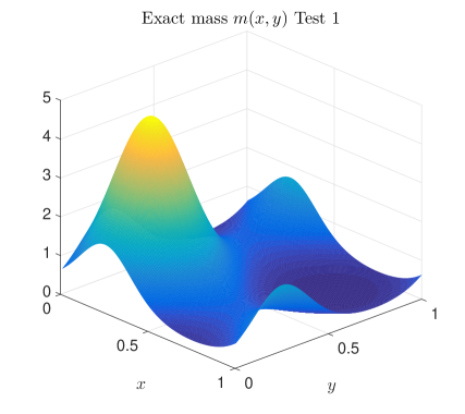
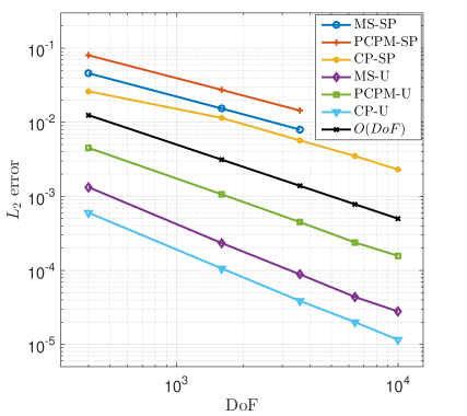
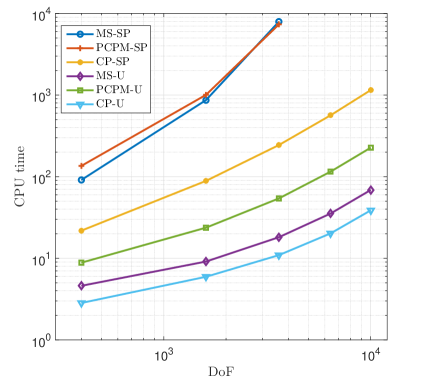
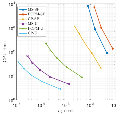
Figure 1: Test 1. Top left: exact mass $m(x,y)$ as in [8]. Top right: convergence rates for the proposed schemes, first-order convergence with respect to the number of nodes is achieved in all the cases. Bottom left: performance plots, degrees of freedom vs. CPU time, the Chambolle-Pock is the fastest algorithm for a fixed mesh parameter $h$. Bottom right: efficiency plots, error vs. CPU time, the Chambolle-Pock algorithm is consistently the most efficient implementation.

In this test, we study the behavior of all the proposed algorithms, for different discretization parameters $h$ and the related number of degrees of freedom $DoF=1/h^{2}$, both in their unsplit and split versions. Results presented in Figure 1 indicate that although all the algorithms achieve the same convergence rate in $h$, measured in the $L^{2}$ norm between the last discrete iteration and the exact solution (4.1), the unsplit versions have smaller error. More importantly, when comparing CPU time (or number of iterations) against $L^{2}$ errors, unsplit algorithms perform considerably better. However, split algorithms are still competitive and provide a reliable way to approximate the solution without performing any matrix inversion. Overall, the Chambolle-Pock algorithm exhibits the best performance and accuracy in both unsplit and split versions. We shall stick to this choice in the following tests.

Test 2: comparing with the ADMM algorithm.

This second text is based on the recent work by [17], where an implementation of the ADMM algorithm is presented for MFG and optimal transportation problems. We compare the performance of the ADMM and the CP-U methods for different discretization parameters and viscosity values $\nu$. For this, the system (1.1) is cast with ${\color[rgb]{1,0,0}F}(x,y,m)=\frac{1}{2}(m-\bar{m}(x,y))^{2}$ and $q=2$, where $\bar{m}(x,y)$ is a Gaussian profile as depicted in Figure 2. In the case $\nu=0$, since our reference $\bar{m}$ is already of mass equal to 1, the exact solution for this problem is given by $u\equiv 0$, $\lambda=0$, and $m=\bar{m}(x)$, and a convergence analysis with respect to this solution is presented in Table 1. From this same table, it can be seen that for different discretization parameters the CP-U algorithm converges to solutions of the same accuracy in a reduced number of iterations. For a fixed discretization, and with varying small viscosity values, the same conclusion is reached in Figure 2. However, as viscosity increases, the ADMM algorithm yields faster computation times than the CP-U implementation (see Table 2).

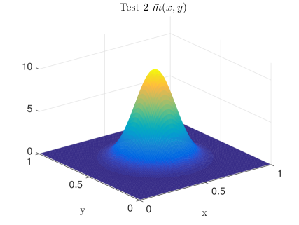
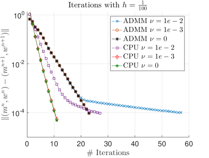
Figure 2: Test 2. Left: reference mass $\bar{m}(x,y)$. Right: iterative behavior of different schemes, for mesh parameter $h=\frac{1}{100}$ and different values of $\nu$. The unsplit Chambolle-Pock algorithm (CP-U) outperforms the ADMM algorithm for low values of $\nu$.

	ADMM			CP-U
DoF	Time	Iterations	$L_{2}$ error	Time	Iterations	$L_{2}$ error
$20^{2}$	1.6 [s]	15	5.42E-4	0.4 [s]	4	1.10E-4
$40^{2}$	3.7 [s]	19	8.44E-5	0.9 [s]	6	9.44E-5
$60^{2}$	21.2 [s]	21	8.16E-5	7.0 [s]	8	9.15E-5
$80^{2}$	33.2 [s]	22	7.92E-5	10.2 [s]	9	8.99E-5
$100^{2}$	87.41 [s]	23	7.35E-5	30.3 [s]	11	7.04E-5

Table 1: Test 2. Different tests with varying number of grid nodes (DoF). Case with $\nu=0$, exact solution $m=\bar{m}(x,y)$. For a similar accuracy, the CP-U algorithm has a reduced number of iterations in comparison to the ADMM routine.

	ADMM		CP-U
$\nu$	Time	Iterations	Time	Iterations
1	8.4 [s]	16	17.5 [s]	46
0.1	30.4[s]	31	65.6 [s]	73
1E-2	26.4 [s]	27	9.8 [s]	11
1E-3	21.3 [s]	21	7.3 [s]	8
0	21.2 [s]	21	7.0 [s]	8

Table 2: Test 2. Different tests with varying viscosity parameter $\nu$. Discretization parameter $h=\frac{1}{60}$. The ADMM algorithm performs better for higher viscosity values, the CP-U algorithm is consistently faster for low viscosities.

Test 3: adding density constraints.

The following test mimics the setting presented in [3], with $q=2$ and

$$f(x,y,m)=m^{2}-\bar{H}(x,y)\,,\quad\bar{H}(x,y)=\sin(2\pi y)+\sin(2\pi x)+\cos(4\pi x)\,.$$

The purpose of this test is twofold. First, in the unconstrained mass case, we reproduce the results presented in [3] and in [23]. As shown in Table 3 (left), we recover the same values for $\lambda$ reported in the aforementioned references. The CP-U algorithm performs consistently well for different viscosity values and reaches convergence after a reduced number of iterations. Computational times are comparable to those reported in [23], considering that the CP-U is a first order method. Next, we perform similar tests but including an upper bound on the mass,

$$m(x,y)\leq d(x,y):=\mathcal{I}_{R}(x,y)+(1-\mathcal{I}_{R}(x,y))\bar{d}\,,\quad\mathcal{I}_{R}(x,y):=\begin{cases}1&x^{2}+y^{2}\leq R^{2}\\ 0&\text{otherwise}\end{cases}\,,\quad\bar{d}=1.3,R=0.25\,.$$

Figure 3 illustrate the effectiveness of our approach, as solutions vary from the unconstrained case in order to satisfy both the MFG system and the additional constraint. The inclusion of mass constraints generate plateau areas where the constraint is active. In Table 3 (right), we observe that the scheme does not deteriorate its performance in the constrained formulation, leading to convergence in a similar number of iterations as in the unconstrained case.

	Unconstrained mass			Constrained mass $m\leq d$
$\nu$	Time	Iterations	$\lambda$	Time	Iterations
1	6.82 [s]	11	0.9786	46.65 [s]	51
0.1	13.26 [s]	27	1.100	13.81 [s]	24
1E-2	34.62 [s]	78	1.1874	29.09 [s]	56
1E-3	22.88 [s]	84	1.1922	27.87 [s]	56

Table 3: Test 3. Performance for the CP-U algorithm in [3] with different viscosity parameter $\nu$, and upper bound on the mass, $m\leq d$. $f(x,y,m)=m^{2}-\bar{H}(x)$. Mesh parameter is set to $h=1/50$. The results for the unconstrained case are in accordance, in accuracy with the values for $\lambda$ presented in [23]. Our scheme performs robustly with respect to the viscosity parameter and the inclusion of mass constraints.

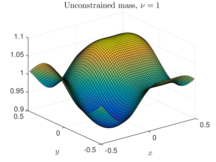
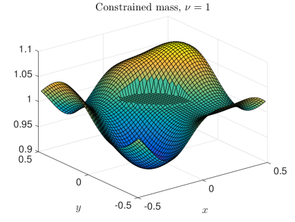
Figure 3: Test 3. Left: unconstrained mass solutions for different viscosity parameters. Right: constrained mass solutions for different viscosity parameters. In both cases the upper bound is selected in order to be active, thus generating a plateau of constant mass.

Test 4: MFG with $q\neq 2$.

In this last test, we further explore the versatility of the proposed framework by considering the same setting as in Test 3 in the unconstrained case with $\nu=1$, but with different values of $q>1$. Results are presented in Figure 4. In general, it can be observed that the performance of the CP-U method remains unaltered, and solutions tend to be uniform when $q$ is close to 1, whereas increasing $q$ leads to sharper solutions with higher extremal values, as shown in Table 4.

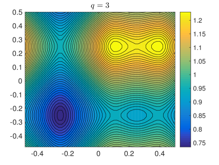
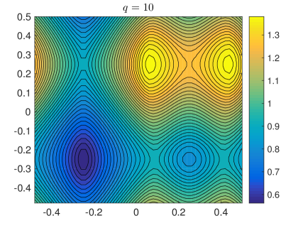
Figure 4: Test 4. Contour plots for the unconstrained mass as in the setting of Test 3, with $\nu=1$. CP-U algorithm with $50^{2}$ nodes. Increasing the value of $q$ generates concentration of mass.

$q$	Time	Iterations	$\min m$	$\max m$
1.2	6.82 [s]	11	0.9989	1.0012
2	6.70 [s]	11	0.9072	1.0737
3	10.57 [s]	21	0.7348	1.2365
10	24.66 [s]	57	0.5628	1.3905

Table 4: Test 4. Performance for the CP-U algorithm and extremal values of the mass.

Concluding Remarks.

In this work we have developed proximal methods for the numerical approximation of stationary Mean Field Games systems. The presented schemes perform efficiently in a series of different tests. In particular, the solution through the Chambolle-Pock algorithm is promising in terms of performance, robustness with respect to the viscosity parameter, and accuracy. A natural extension of this work is its application for the approximation of time-dependent case, and the further study of the different features of the approach, which allows constraints on the mass and the modeling of congested transport.

Acknowledgments.

The first author thanks the support of CONICYT through grants FONDECYT 11140360, MathAmSud 15MATH02, and ECOS-CONICYT C13E03. The second author thanks the support of ERC-Advanced Grant OCLOC:“From Open-Loop to Closed-Loop Optimal Control of PDEs”. The third author thanks the support from project iCODE :“Large-scale systems and Smart grids: distributed decision making” and from the Gaspar Monge Program for Optimization and Operation Research (PGMO).

Appendix

4.1 Proof of Theorem 3.1

Proof. In order to simplify the proof we will consider the case $\theta=1$ as in [31]. Fix $k\in\mathbb{N}$, let $\hat{y}\in C$ and $\hat{\sigma}\in\mathbb{R}^{M}$ be a primal-dual solution to (3.5)-(3.6). It follows from $P_{C}\hat{y}=\hat{y}$ and (3.9) that

$$\frac{|y^{k+1}-\hat{y}|^{2}}{2\tau}+\frac{|\sigma^{k+1}-\hat{\sigma}|^{2}}{2\gamma} \leq\frac{1}{2\tau}\Big{(}|p^{k+1}-\hat{y}|^{2}-|p^{k+1}-y^{k+1}|^{2}\Big{)}+\frac{|\sigma^{k+1}-\hat{\sigma}|^{2}}{2\gamma}$$

$$\leq\frac{1}{2\tau}\Big{(}|y^{k}-\hat{y}-\tau\Xi^{*}(\sigma^{k+1}-\hat{\sigma})|^{2}-|y^{k}-p^{k+1}-\tau\Xi^{*}(\sigma^{k+1}-\hat{\sigma})|^{2}$$

$$\hskip 213.39566pt-|p^{k+1}-y^{k+1}|^{2}\Big{)}$$

$$\hskip 14.22636pt+\frac{1}{2\gamma}\Big{(}|\sigma^{k}-\hat{\sigma}+\gamma\Xi(\bar{y}^{k}-\hat{y})|^{2}-|\sigma^{k}-\sigma^{k+1}+\gamma\Xi(\bar{y}^{k}-\hat{y})|^{2}$$

$$=\frac{1}{2\tau}\Big{(}|y^{k}-\hat{y}|^{2}-2\tau{{({p^{k+1}-\hat{y}})\cdot({\Xi^{*}(\sigma^{k+1}-\hat{\sigma})})}}-|y^{k}-p^{k+1}|^{2}$$

$$\hskip 213.39566pt-|p^{k+1}-y^{k+1}|^{2}\Big{)}$$

$$\hskip 14.22636pt+\frac{1}{2\gamma}\Big{(}|\sigma^{k}-\hat{\sigma}|^{2}+2\gamma{{({\sigma^{k+1}-\hat{\sigma}})\cdot({\Xi(\bar{y}^{k}-\hat{y})})}}-|\sigma^{k}-\sigma^{k+1}|^{2}$$

$$=\frac{|y^{k}-\hat{y}|^{2}}{2\tau}+\frac{|\sigma^{k}-\hat{\sigma}|^{2}}{2\gamma}-\frac{|y^{k}-p^{k+1}|^{2}}{2\tau}-\frac{|\sigma^{k}-\sigma^{k+1}|^{2}}{2\gamma}$$

$$\hskip 14.22636pt-{{({\Xi(p^{k+1}-\hat{y})})\cdot({\sigma^{k+1}-\hat{\sigma}})}}+{{({\sigma^{k+1}-\hat{\sigma}})\cdot({\Xi(\bar{y}^{k}-\hat{y})})}}$$

$$\hskip 14.22636pt-\frac{|p^{k+1}-y^{k+1}|^{2}}{2\tau}$$

$$=\frac{|y^{k}-\hat{y}|^{2}}{2\tau}+\frac{|\sigma^{k}-\hat{\sigma}|^{2}}{2\gamma}-\frac{|y^{k}-p^{k+1}|^{2}}{2\tau}-\frac{|\sigma^{k}-\sigma^{k+1}|^{2}}{2\gamma}$$

$$\hskip 14.22636pt+{{({\sigma^{k+1}-\hat{\sigma}})\cdot({\Xi(\bar{y}^{k}-{p}^{k+1})})}}-\frac{|p^{k+1}-y^{k+1}|^{2}}{2\tau}.$$ (4.2)

Since we are assuming, for simplicity, $\theta=1$, we have $\bar{y}^{k}=y^{k}+p^{k}-y^{k-1}$, which yields

$${{({\sigma^{k+1}-\hat{\sigma}})\cdot({\Xi(\bar{y}^{k}-{p}^{k+1})})}} ={{({\sigma^{k+1}-\hat{\sigma}})\cdot({\Xi(y^{k}-{p}^{k+1})})}}+{{({\sigma^{k+1}-\hat{\sigma}})\cdot({\Xi(p^{k}-{y}^{k-1})})}}$$

$$=-{{({\sigma^{k+1}-\hat{\sigma}})\cdot({\Xi({p}^{k+1}-y^{k})})}}+{{({\sigma^{k}-\hat{\sigma}})\cdot({\Xi(p^{k}-{y}^{k-1})})}}$$

$$\hskip 128.0374pt+{{({\sigma^{k+1}-\sigma^{k}})\cdot({\Xi(p^{k}-{y}^{k-1})})}}$$

$$\leq-{{({\sigma^{k+1}-\hat{\sigma}})\cdot({\Xi({p}^{k+1}-y^{k})})}}+{{({\sigma^{k}-\hat{\sigma}})\cdot({\Xi(p^{k}-{y}^{k-1})})}}$$

$$\hskip 128.0374pt+\|\Xi\|\,|\sigma^{k+1}-\sigma^{k}|\,|p^{k}-{y}^{k-1}|$$

$$\leq-{{({\sigma^{k+1}-\hat{\sigma}})\cdot({\Xi({p}^{k+1}-y^{k})})}}+{{({\sigma^{k}-\hat{\sigma}})\cdot({\Xi(p^{k}-{y}^{k-1})})}}$$

$$\hskip 71.13188pt+\sqrt{\gamma\tau}\|\Xi\|\frac{|\sigma^{k+1}-\sigma^{k}|^{2}}{2\gamma}+\sqrt{\gamma\tau}\|\Xi\|\frac{|p^{k}-{y}^{k-1}|^{2}}{2\tau}.$$ (4.3)

Therefore, from (4.1) we obtain

$$\frac{|y^{k+1}-\hat{y}|^{2}}{2\tau}+\frac{|\sigma^{k+1}-\hat{\sigma}|^{2}}{2\gamma} \leq\frac{|y^{k}-\hat{y}|^{2}}{2\tau}+\frac{|\sigma^{k}-\hat{\sigma}|^{2}}{2\gamma}-\frac{|y^{k}-p^{k+1}|^{2}}{2\tau}+\frac{|{y}^{k-1}-p^{k}|^{2}}{2\tau}$$

$$\hskip 14.22636pt-(1-\sqrt{\gamma\tau}\|\Xi\|)\left(\frac{|{y}^{k-1}-p^{k}|^{2}}{2\tau}+\frac{|\sigma^{k+1}-\sigma^{k}|^{2}}{2\gamma}\right)$$

$$\hskip 14.22636pt-\frac{|p^{k+1}-y^{k+1}|^{2}}{2\tau}$$

$$\hskip 14.22636pt-{{({\sigma^{k+1}-\hat{\sigma}})\cdot({\Xi({p}^{k+1}-y^{k})})}}+{{({\sigma^{k}-\hat{\sigma}})\cdot({\Xi(p^{k}-{y}^{k-1})})}}$$ (4.4)

By calling

$$a^{k} =\frac{|\sigma^{k+1}-\hat{\sigma}|^{2}}{2\gamma}+{{({\sigma^{k+1}-\hat{\sigma}})\cdot({\Xi(y^{k}-{p}^{k+1})})}}+\frac{|y^{k}-p^{k+1}|^{2}}{2\tau}$$

$$\geq\frac{|\sigma^{k+1}-\hat{\sigma}|^{2}}{2\gamma}+{{({\sigma^{k+1}-\hat{\sigma}})\cdot({\Xi(y^{k}-{p}^{k+1})})}}+\frac{\gamma\|\Xi\|^{2}|y^{k}-p^{k+1}|^{2}}{2}$$

$$\geq\frac{1}{2\gamma}\left(|\sigma^{k+1}-\hat{\sigma}|^{2}+2{{({\sigma^{k+1}-\hat{\sigma}})\cdot({\gamma\Xi(y^{k}-{p}^{k+1})})}}+|\gamma\Xi(y^{k}-p^{k+1})|^{2}\right)$$

$$=\frac{1}{2\gamma}|\sigma^{k+1}-\hat{\sigma}+\gamma\Xi(y^{k}-{p}^{k+1})|^{2}\geq 0,$$ (4.5)

it follows from (4.1) that

$$\frac{|y^{k+1}-\hat{y}|^{2}}{2\tau}+a^{k+1} \leq\frac{|y^{k}-\hat{y}|^{2}}{2\tau}+a^{k}-(1-\sqrt{\gamma\tau}\|\Xi\|)\left(\frac{|{y}^{k-1}-p^{k}|^{2}}{2\tau}+\frac{|\sigma^{k+1}-\sigma^{k}|^{2}}{2\gamma}\right)$$

$$\hskip 14.22636pt-\frac{|p^{k+1}-y^{k+1}|^{2}}{2\tau}$$ (4.6)

and, hence, $(\frac{|y^{k}-\hat{y}|^{2}}{2\tau}+a^{k})_{k\in\mathbb{N}}$ is a Fejér sequence and, from [12, Lemma 3.1(iii)] we have

$$y^{k-1}-p^{k}\to 0,\>\sigma^{k+1}-\sigma^{k}\to 0,\>p^{k}-y^{k}\to 0$$ (4.7)

and there exists $\alpha\geq 0$ such that $\frac{|y^{k}-\hat{y}|^{2}}{2\tau}+a^{k}\to\alpha$. It follows from (4.1) that

$$\left|a^{k}-\frac{|\sigma^{k+1}-\hat{\sigma}|^{2}}{2\gamma}\right|\leq\|\Xi\|\,|\sigma^{k+1}-\hat{\sigma}|\,|y^{k}-{p}^{k+1}|+\frac{|y^{k}-p^{k+1}|^{2}}{2\tau}\to 0,$$ (4.8)

which yields

$$\xi^{k}(\hat{y},\hat{\sigma}):=\frac{|y^{k}-\hat{y}|^{2}}{2\tau}+\frac{|\sigma^{k+1}-\hat{\sigma}|^{2}}{2\gamma}=\frac{|y^{k}-\hat{y}|^{2}}{2\tau}+a^{k}+\frac{|\sigma^{k+1}-\hat{\sigma}|^{2}}{2\gamma}-a^{k}\to\alpha.$$ (4.9)

Hence, we have from (4.1) that $(y^{k})_{k\in\mathbb{N}}$ and $(\sigma^{k})_{k\in\mathbb{N}}$ are bounded. Let $\bar{y}$ and $\bar{\sigma}$ be accumulation points of the sequences $(y^{k})_{k\in\mathbb{N}}$ and $(\sigma^{k})_{k\in\mathbb{N}}$, respectively, say $y^{k_{n}}\to\bar{y}$ and $\sigma^{k_{n}}\to\bar{\sigma}$. It follows from (4.7) that $\sigma^{k_{n}+1}\to\bar{\sigma}$, $p^{k_{n}}\to\bar{y}$, $p^{k_{n}+1}\to\bar{y}$, $y^{k_{n}-1}\to\bar{y}$ and $\bar{y}^{k_{n}}=y^{k_{n}}+p^{k_{n}}-y^{k_{n}-1}\to\bar{y}$. Hence, since $\operatorname{prox}_{\gamma\psi*}$, $\operatorname{prox}_{\tau\varphi}$, and $P_{C}$ are continuous, by passing through the limit in (3.1), we obtain $\bar{y}\in C$ and

$$\begin{cases}\operatorname{prox}_{\tau\varphi}(\bar{y}-\tau\Xi^{*}\bar{\sigma})=\bar{y}\\ \operatorname{prox}_{\gamma\psi^{*}}(\bar{\sigma}+\gamma\Xi\bar{y})=\bar{\sigma},\end{cases}$$ (4.10)

and, from (3.9), $(\bar{y},\bar{\sigma})$ is a primal-dual solution to (3.5). It is enough to prove that there is only one accumulation point. By contradiction, suppose that $(\bar{y}_{1},\bar{\sigma}_{1})$ and $(\bar{y}_{2},\bar{\sigma}_{2})$ are two accumulation points, say $(y^{k_{n}},\sigma^{k_{n}})\to(\bar{y}_{1},\bar{\sigma}_{1})$ and $(y^{k_{m}},\sigma^{k_{m}})\to(\bar{y}_{2},\bar{\sigma}_{2})$. Since any accumulation point is a solution, we deduce from (4.9) that there exist $\alpha_{1}\geq 0$ and $\alpha_{2}\geq 0$ such that $\xi^{k}(\bar{y}_{1},\bar{\sigma}_{1})\to\alpha_{1}$ and $\xi^{k}(\bar{y}_{2},\bar{\sigma}_{2})\to\alpha_{2}$. Now, for every $k\in\mathbb{N}$,

$$\xi^{k}(\bar{y}_{1},\bar{\sigma}_{1}) =\frac{|y^{k}-\bar{y}_{1}|^{2}}{2\tau}+\frac{|\sigma^{k+1}-\bar{\sigma}_{1}|^{2}}{2\gamma}$$

$$=\xi^{k}(\bar{y}_{2},\bar{\sigma}_{2})+\frac{1}{\tau}{{({y^{k}-\bar{y}_{2}})\cdot({\bar{y}_{2}-\bar{y}_{1}})}}$$

$$\hskip 28.45274pt+\frac{1}{\gamma}{{({\sigma^{k}-\bar{\sigma}_{2}})\cdot({\bar{\sigma}_{2}-\bar{\sigma}_{1}})}}+\frac{|\bar{y}_{1}-\bar{y}_{2}|^{2}}{2\tau}+\frac{|\bar{\sigma}_{1}-\bar{\sigma}_{2}|^{2}}{2\gamma}$$ (4.11)

Then, we have

$$\frac{1}{\tau}{{({y^{k}})\cdot({\bar{y}_{2}-\bar{y}_{1}})}}+\frac{1}{\gamma}{{({\sigma^{k}})\cdot({\bar{\sigma}_{2}-\bar{\sigma}_{1}})}} =\xi^{k}(\bar{y}_{1},\bar{\sigma}_{1})+\frac{1}{\tau}{{({\bar{y}_{2}})\cdot({\bar{y}_{2}-\bar{y}_{1}})}}+\frac{1}{\gamma}{{({\bar{\sigma}_{2}})\cdot({\bar{\sigma}_{2}-\bar{\sigma}_{1}})}}$$

$$-\frac{|\bar{y}_{1}-\bar{y}_{2}|^{2}}{2\tau}-\frac{|\bar{\sigma}_{1}-\bar{\sigma}_{2}|^{2}}{2\gamma}-\xi^{k}(\bar{y}_{2},\bar{\sigma}_{2})\to\ell,$$ (4.12)

where $\ell:=\alpha_{1}-\alpha_{2}+\frac{1}{\tau}{{({\bar{y}_{2}})\cdot({\bar{y}_{2}-\bar{y}_{1}})}}+\frac{1}{\gamma}{{({\bar{\sigma}_{2}})\cdot({\bar{\sigma}_{2}-\bar{\sigma}_{1}})}}-\frac{|\bar{y}_{1}-\bar{y}_{2}|^{2}}{2\tau}-\frac{|\bar{\sigma}_{1}-\bar{\sigma}_{2}|^{2}}{2\gamma}$. Finally, by taking in particular the subsequences $(k_{n})_{n\in\mathbb{N}}$ and $(k_{m})_{m\in\mathbb{N}}$ we obtain

$$\frac{1}{\tau}{{({\bar{y}_{1}})\cdot({\bar{y}_{2}-\bar{y}_{1}})}}+\frac{1}{\gamma}{{({\bar{\sigma}_{1}})\cdot({\bar{\sigma}_{2}-\bar{\sigma}_{1}})}} =\lim_{n\in\mathbb{N}}\frac{1}{\tau}{{({y^{k_{n}}})\cdot({\bar{y}_{2}-\bar{y}_{1}})}}+\frac{1}{\gamma}{{({\sigma^{k_{n}}})\cdot({\bar{\sigma}_{2}-\bar{\sigma}_{1}})}}$$

$$=\ell$$

$$=\lim_{m\in\mathbb{N}}\frac{1}{\tau}{{({y^{k_{m}}})\cdot({\bar{y}_{2}-\bar{y}_{1}})}}+\frac{1}{\gamma}{{({\sigma^{k_{m}}})\cdot({\bar{\sigma}_{2}-\bar{\sigma}_{1}})}}$$

$$=\frac{1}{\tau}{{({\bar{y}_{2}})\cdot({\bar{y}_{2}-\bar{y}_{1}})}}+\frac{1}{\gamma}{{({\bar{\sigma}_{2}})\cdot({\bar{\sigma}_{2}-\bar{\sigma}_{1}})}},$$ (4.13)

which yields $|\bar{y}_{2}-\bar{y}_{1}|^{2}/\tau+|\bar{\sigma}_{2}-\bar{\sigma}_{1}|^{2}/\gamma=0$ and the result follows.

References

- [1] Y. Achdou, F. Camilli, and I. Capuzzo Dolcetta. Mean field games: Numerical methods for the planning problem. SIAM J. Control Optim., 50:79–109, 2012.
- [2] Y. Achdou, F. Camilli, and I. Capuzzo Dolcetta. Mean field games: convergence of a finite difference method. SIAM J. Numer. Anal., 51(5):2585–2612, 2013.
- [3] Y. Achdou and I. Capuzzo Dolcetta. Mean field games: Numerical methods. SIAM J. Numer. Anal., 48(3):1136–1162, 2010.
- [4] Y. Achdou and V. Perez. Iterative strategies for solving linearized discrete mean field games systems. Netw. Heterog. Media, 7(2):197–217, 2012.
- [5] Y. Achdou and A. Porretta. Convergence of a finite difference scheme to weak solutions of the system of partial differential equations arising in mean field games. SIAM J. Numer. Anal., 54(1):161–186, 2016.
- [6] G. Albi, Y. P. Choi, M Fornasier, and D. Kalise. Mean field control hierarchy. RICAM Report 16-25, 2016.
- [7] N. Almayouf, E. Bachini, A. Chapouto, R. Ferreira, D.-A. Gomes, D. Jordao, D.-E. Junior, A. Karagulyan, J. Monasterio, L. Nurbekyan, G. Pagliar, M. Piccirilli, S. Pratapsi, M. Prazeres, J. Reis, A. Rodrigues, O. Romero, M. Sargsyan, T. Seneci, C. Song, K. Terai, R. Tomisaki, H. Velasco-Perez, V. Voskanyan, and X. Yang. Existence of positive solutions for an approximation of stationary mean-field games. Preprint, 2015.
- [8] N. Almulla, R. Ferreira, and D.-A. Gomes. Two numerical approaches to stationary mean-field games. Preprint, 2015.
- [9] R. Andreev. Preconditioning the augmented lagrangian method for instationary mean field games with diffusion. hal-01301282, 2016.
- [10] H. Attouch, G. Buttazzo, and G. Michaille. Variational analysis in Sobolev and BV spaces. Applications to PDEs and optimization. MPS/SIAM Series on Optimization, (SIAM), Philadelphia, (2006).
- [11] M. Bardi and E. Feleqi. Nonlinear elliptic systems and mean field games. Preprint, 2015.
- [12] H. H. Bauschke and P. L. Combettes. Quasi-Fejérian analysis of some optimization algorithms. in Inherently Parallel Algorithms in Feasibility and Optimization and Their Applications (D. Butnariu, Y. Censor, and S. Reich, Eds.), pages 115–152, 2001.
- [13] H. H. Bauschke and P. L. Combettes. Convex Analysis and Monotone Operator Theory in Hilbert Spaces. Springer, New York, 2011.
- [14] H. H. Bauschke and P. L. Combettes. Convex Analysis and Monotone Operator Theory in Hilbert Spaces. Springer-Verlag, New York, 2011.
- [15] A. Beck and M. Teboulle. A fast iterative shrinkage-thresholding algorithm for linear inverse problems. SIAM J. Imaging Sci., 2-1:183–202, 2009.
- [16] J.-D. Benamou and Y. Brenier. A computational fluid mechanics solution to the Monge-Kantorovich mass transfer problem. Numer. Math., 84(3):375–393, 2000.
- [17] J.-D. Benamou and G. Carlier. Augmented lagrangian methods for transport optimization, mean field games and degenerate elliptic equations. Journal of Optimization Theory and Applications, 167:1–26, 2015.
- [18] J.-D. Benamou, G. Carlier, and F. Santambrogio. Variational mean field games. Preprint, 2016.
- [19] S. Boyd, N. Parikh, E. Chu, B. Peleato, and J. Eckstein. Distributed optimization and statistical learning via the alternating direction method of multipliers. Found. Trends Mach. Learn., 3(1):1–122, 2011.
- [20] L. M. Briceño-Arias and P. L. Combettes. A monotone+skew splitting model for composite monotone inclusions in duality. SIAM J. Optim., 21:1230–1250, 2011.
- [21] M. Burger, M. Di Francesco, P.A. Markowich, and M.T. Wolfram. Mean field games with nonlinear mobilities in pedestrian dynamics. Discrete and Continuous Dynamical Systems - B, 19(5):1311–1333, 2014.
- [22] G. Buttazzo, C. Jimenez, and E. Oudet. An optimization problem for mass transportation with congested dynamics. SIAM J. Control Optim., 48(3):1961–1976, 2009.
- [23] S. Cacace and F. Camilli. Ergodic problems for Hamilton-Jacobi equations: yet another but efficient numerical method. arXiv:1601.07107, 2016.
- [24] F. Camilli and F. Silva. A semi-discrete approximation for a first order mean field game problem. Networks and Heterogeneous Media, 7(2):263–277, 2012.
- [25] P. Cardaliaguet. Long time average of first order mean field games and weak KAM theory. Dynamic Games and Applications, 3:473–488, 12 2013.
- [26] P. Cardaliaguet and P. J. Graber. Mean field games systems of first order. ESAIM: Control Optim. Calc. Var., 21(3):690–722, 2015.
- [27] P. Cardaliaguet, J.-M. Lasry, P.-L. Lions, and A. Porretta. Long time average of mean field games. Networks and Heterogeneous Media, AIMS, 7(2):279–301, 2012.
- [28] P. Cardaliaguet, J.-M. Lasry, P.-L. Lions, and A. Porretta. Long time average of mean field games with a nonlocal coupling. SIAM J. Control Optim., 51(5):3558–3591, 2013.
- [29] E. Carlini and F. J. Silva. A Fully Discrete Semi-Lagrangian scheme for a first order mean field game problem. SIAM J. Numer. Anal., 52(1):45–67, 2014.
- [30] E. Carlini and F. J. Silva. A Semi-Lagrangian scheme for a degenerate second order mean field game system. Discrete and Continuous Dynamical Systems, 35(9):4269–4292, 2015.
- [31] A. Chambolle and T. Pock. A first order primal dual algorithm for convex problems with applications to imaging. J. Math. Imaging Vis., 40:120–145, 2011.
- [32] G. Chen and M. Teboulle. A proximal-based decomposition method for convex minimization problems. Math. Programming Ser. A, 64:81–101, 1994.
- [33] M. Cirant. Multi-population mean field games systems with Neumann boundary conditions. J. Math. Pures Appl. (9), 103(5):1294–1315, 2015.
- [34] M. Cirant. Stationary focusing mean-field games. Communications in Partial Differential Equations, 41(8):1324–1346, 2016.
- [35] P. L. Combettes and V. R. Wajs. Signal recovery by proximal forward-backward splitting. Multiscale Model. Simul., 4:1168–1200, 2005.
- [36] J. Eckstein. Splitting methods for monotone operators with applications to parallel optimization. PhD thesis, MIT, 1989.
- [37] J. Eckstein and D. Bertsekas. On the Douglas-Rachford splitting method and the proximal point algorithm for maximal monotone operators. Math. Programming, 55:293–318, 1992.
- [38] I. Ekeland and R. Temam. Analyse convexe et problèmes variationnels. Collection Études Mathématiques. Dunod; Gauthier-Villars, Paris-Brussels-Montreal, Que., 1974.
- [39] R. Ferreira and D.-A. Gomes. Existence of weak solutions to stationary mean-field games through variational inequalities. arXiv:1512.05828., 2016.
- [40] D. Gabay. Applications of the method of multipliers to variational inequalities. In Michel Fortin and Roland Glowinski, editors, Augmented Lagrangian Methods: Applications to the Numerical Solution of Boundary-Value Problems, volume 15 of Studies in Mathematics and Its Applications, pages 299 – 331. Elsevier, 1983.
- [41] D. Gabay and B. Mercier. A dual algorithm for the solution of nonlinear variational problems via finite element approximation. Computers and Mathematics with Applications, 2(1):17–40, 1976.
- [42] R. Glowinski and A. Marrocco. Sur l’approximation, par éléments finis d’ordre un, et la résolution, par pénalisation-dualité, d’une classe de problèmes de Dirichlet non linéaires. Rev. Française Automat. Informat. Recherche Opérationnelle Sér. Rouge Anal. Numér., 9(R-2):41–76, 1975.
- [43] D.-A. Gomes and H. Mitake. Existence for stationary mean-field games with congestion and quadratic Hamiltonians. NoDEA Nonlinear Differential Equations Appl., 22(6):1897–1910, 2015.
- [44] D.-A. Gomes, J. Mohr, and R. Souza. Discrete time, finite state space mean field games,. J. Math. Pures Appl. (9), 93(3):308–328, 2010.
- [45] D.-A. Gomes, S. Patrizi, and V. Voskanyan. On the existence of classical solutions for stationary extended mean field games. Nonlinear Anal., 99:49–79, 2014.
- [46] D.-A. Gomes, G.-E. Pires, and H. Sánchez-Morgado. A-priori estimates for stationary mean-field games. Netw. Heterog. Media, 7(2):303–314, 2012.
- [47] M. R. Hestenes. Multiplier and gradient methods. In Computing Methods in Optimization Problems, 2 (Proc. Conf., San Remo, 1968), pages 143–163. Academic Press, New York, 1969.
- [48] M. R. Hestenes. Multiplier and gradient methods. J. Optim. Theory Appl., 4:303–320, 1969.
- [49] M. Huang, P. E. Caines, and R. P. Malhamé. Large-population cost-coupled LQG problems with nonuniform agents: individual-mass behavior and decentralized -Nash equilibria. IEEE Trans. Automat. Control, 52(9):1560–1571, 2007.
- [50] A. Lachapelle, J. Salomon, and G. Turinici. Computation of mean field equilibria in economics. Mathematical Models and Methods in Applied Sciences, 20(4):567–588, 2010.
- [51] J.-M. Lasry and P.-L. Lions. Jeux à champ moyen I. Le cas stationnaire. C. R. Math. Acad. Sci. Paris, 343:619–625, 2006.
- [52] J.-M. Lasry and P.-L. Lions. Jeux à champ moyen II. Horizon fini et contrôle optimal. C. R. Math. Acad. Sci. Paris, 343:679–684, 2006.
- [53] J.-M. Lasry and P.-L. Lions. Mean field games. Jpn. J. Math., 2:229–260, 2007.
- [54] B. Martinet. Régularisation d’inéquations variationnelles par approximations successives. Rev. Française Informat. Recherche Opérationnelle, 4(3):154–158, 1970.
- [55] B. Maury, A. Roudneff-Chupin, and F. Santambrogio. A macroscopic crowd motion model of gradient flow type. Math. Models Methods Appl. Sci., 20(10):1787–1821, 2010.
- [56] B. Maury, A. Roudneff-Chupin, and F. Santambrogio. Congestion-driven dendritic growth. Discrete Contin. Dyn. Syst., 34(4):1575–1604, 2014.
- [57] A. R. Mészáros and F. J. Silva. A variational approach to second order mean field games with density constraints: The stationary case. J. Math. Pures Appl. (9), 104(6):1135–1159, 2015.
- [58] Yu. Nesterov. A method for solving the convex programming problem with convergence rate . Dokl. Akad. Nauk SSSR, 269(3):543–547, 1983.
- [59] Yu. Nesterov. Smooth minimization of non-smooth functions. Math. Program. Ser. A, 103(1):127–152, 2005.
- [60] N. Papapdakis, G. Peyré, and E. Oudet. Optimal transport with proximal splitting. SIAM J. Imaging Sci., 7:212–238, 2014.
- [61] E.-A Pimentel and V. Voskanyan. Regularity for second order stationary mean-field games. arXiv:1503.06445, 2015.
- [62] M. J. D. Powell. A method for nonlinear constraints in minimization problems. In Optimization (Sympos., Univ. Keele, Keele, 1968), pages 283–298. Academic Press, London, 1969.
- [63] R. T. Rockafellar. Convex analysis. Princeton Mathematical Series, No. 28. Princeton University Press, Princeton, N.J., 1970.
- [64] R. T. Rockafellar. Monotone operators and the proximal point algorithm. SIAM J. Control Optimization, 14(5):877–898, 1976.
- [65] F. Santambrogio. A modest proposal for MFG with density constraints. Netw. Heterog. Media, 7(2):337–347, 2012.
- [66] F. Santambrogio. Optimal Transport for Applied Mathematicians: Calculus of Variations, PDEs, and Modeling. Progress in Nonlinear Differential Equations and Their Applications. Birkhäuser, 2015.
- [67] P. Tseng. A modified forward-backward splitting method for maximal monotone mappings. SIAM J. Control Optim., 38:431–446, 2000.