On the Magnetic and Energy Characteristics of Recurrent Homologous Jets from An Emerging Flux

Abstract

In this paper, we present the detailed analysis of recurrent homologous jets originating from an emerging negative magnetic flux at the edge of an Active Region.The observed jets show multi-thermal features. Their evolution shows high consistence with the characteristic parameters of the emerging flux, suggesting that with more free magnetic energy, the eruptions tend to be more violent, frequent and blowout-like. The average temperature, average electron number density and axial speed are found to be similar for different jets, indicating that they should have been formed by plasmas from similar origins. Statistical analysis of the jets and their footpoint region conditions reveals a strong positive relationship between the footpoint-region total 131 Å intensity enhancement and jets’ length/width. Stronger linearly positive relationships also exist between the total intensity enhancement/thermal energy of the footpoint regions and jets’ mass/kinetic/thermal energy, with higher cross-correlation coefficients. All the above results, together, confirm the direct relationship between the magnetic reconnection and the jets, and validate the important role of magnetic reconnection in transporting large amount of free magnetic energy into jets. It is also suggested that there should be more free energy released during the magnetic reconnection of blowout than of standard jet events.

1 Introduction

Solar jets are bulks of plasma material ejected along elongated trajectories from the solar surface. They are one of the most common dynamic phenomena occuring within the solar atmosphere and could be found in active, quiet-Sun and polar regions. Based on their spatial scales, jets may be divided into two classes: large-scale and small-scale jets. Small-scale jets are ubiquitous and, here, include type-I and type-II spicules (the latter also referred to as rapid blue excursions, RBEs) in the chromosphere/transition region [e.g., Beckers, 1968; Sterling, 2000; De Pontieu et al., 2007; van der Voort et al., 2009; Cranmer and Woolsey, 2015; Kuridze et al., 2015] and quasi-periodic intensity perturbations in the corona [e.g., Verwichte et al., 2009; Threlfall et al., 2013; Liu et al., 2015a]. The importance of small-scale jets are well-known as they are suggested to contribute to coronal heating and/or solar wind acceleration [e.g., Shibata et al., 2007; Moore et al., 2011; Tian et al., 2014].

Compared with small-scale jets, large-scale jets are more evident, even observable by lower-resolution instruments like STEREO/EUVI and SOHO/EIT. Based on their different dominant temperatures, large-scale jets are sometimes referred to as H$\alpha$ surges with cold plasmas [e.g., Roy, 1973; Canfield et al., 1996], UV/EUV jets or macrospicules with warm plasmas [e.g., Bohlin et al., 1975; Liu et al., 2014; Bennett and Erdélyi, 2015], X-ray jets with hot plasmas [e.g., Shibata et al., 1992; Cirtain et al., 2007] and white-light jets seen in white-light coronagraph [e.g., Moore et al., 2015; Liu et al., 2015b; Zheng et al., 2016]. The above classification is approximate and not absolute, because jets are often found to be formed of multi-thermal plasmas and thus observed in multi-passbands. Attributed to observational facts of jets including their “Reverse-Y” shape and the accompanied nano-flares (or brightening), it is now widely believed that large-scale jets are most likely to be triggered by magnetic reconnection, especially the interchange reconnection between closed and (locally) open magnetic field lines [see, e.g., Shibata et al., 1996; Scullion et al., 2009; Pariat et al., 2015].

In simulations, free magnetic energy can be introduced by at least two ways preceding the eruption of jets: flux emergence/cancellation [e.g., Moreno-Insertis et al., 2008; Murray et al., 2009; Fang et al., 2014], or rotational/shearing motion at the footpoint region [e.g., Pariat et al., 2009; Yang et al., 2013]. In the first scenario, reconnection happens between the pre-existing open flux and newly emerging closed flux. To ensure the onset of magnetic reconnection, the emerging flux should contain certain amount of free magnetic energy or a persistent Poynting flow from below the photosphere to inject the energy. It is then not surprising recurrent jets might be triggered by repeated magnetic reconnection during the emergence of magnetic flux [e.g. Chen et al., 2015]. However, the question, that how the occurence of recurrent jets is influenced by the emerging flux in observations, still needs to be addressed.

As efforts in studying recurrent jets [e.g., Pariat et al., 2010; Chen et al., 2015] from observational perspectives, Guo et al. [2013], Zhang and Ji [2014] and Li et al. [2015] studied the photospheric current patterns, successive blobs and the quasi-periodic behavior of recurrent jets from newly emerging fluxes at the edge of three different active regions, respectively. Archontis et al. [2010] performed a 3D MHD numerical simulation in which a small active region is constructed by the emergence of a toroidal magnetic flux tube. As a result of the new emerging flux, successive magnetic reconnections set in and a series of recurrent jets erupt. The above studies all support the importance of magnetic reconnection in triggering recurrent jets. The natural question arises: how much the reconnection influences the properties (such as length, width and mass etc.) of jets in observations is vital to understanding the related physical processes. Moreover, statistical study of the relations between the energies of jets and of the corresponding footpoint regions will help us explore how free magnetic energy is distributed during magnetic reconnection.

In this paper, we will perform a statistical analysis of recurrent homologous jets from one emerging (negative) flux at the edge of a part with positive magnetic field of an active region. Study on the evolution of the photospheric magnetic field SDO/HMI observations is shown in Sect. 2. A combined analysis on the jets observed by SDO/AIA and several characteristic magnetic parameters including the photospheric mean current density, the mean current helicity, and the total photospheric free magnetic energy is performed in Sect. 3 and 4 to investigate the synchronism between the evolution of the jets and their magnetic field conditions at footpoints. In Sect. 5 and 6, we present the statistical studies of the properties of jets and their corresponding footpoint regions. Our study will be summarized in Sect. 7.

2 The Photospheric Magnetic Field

Jets studied in this paper are found to be related to an emerging negative polarity at the north-east edge of Active Region NOAA 12301 from around 03:00 UT to 12:00 UT on July 9th 2015. This Active Region, with a large-scale quadrupolar configuration (for a small landscape in Figure 1(a)), turns to the front with a very small positive latitude on late July 3rd and is almost at the central meridian during the time window from 03:00 UT to 12:00 UT on July 9th. Besides the line-of-sight (LOS) magnetic field from SDO/HMI (Fig. 1(a)), vector magnetic field data is also available for this Active Region by the Space-weather HMI Active Region Patches [SHARPs, Bobra et al., 2014] with SHARP NO. 5745.

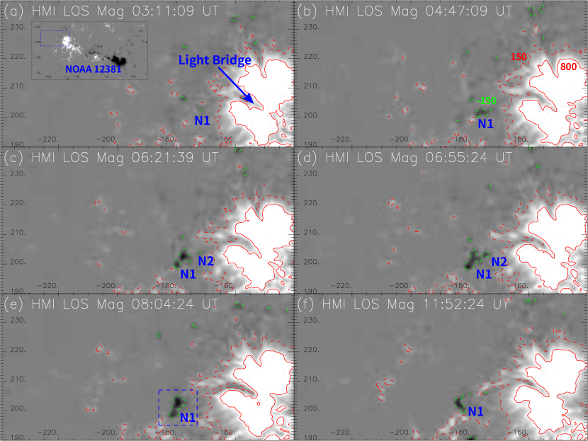
Figure 1: Temporal evolution of the emerging negative flux (“N1”) and nearby positive polarity (the main polarity) of Active Region NOAA 12301 observed by the SDO/HMI instrument from 03:00 UT to 12:00 UT. The blue dashed box in the small landscape in panel (a) defines the scope of all the panels from (a) to (f). Red solid and dashed curves indicate LOS magnetic field levels at 800 G and 150 G respective, with the green curves -150 G. Blue dashed box in panel (e) covers the region of the emerging negative polarity which results in more than ten times of jet eruptions. Coordinates are in units of arc second.

Figure 1 shows the evolution of the northern part with of the Active Region and the nearby emerging negative polarities during the aforementioned period. All HMI observations have been de-rotated to 00:00 UT. Solid and dashed red curves in all the panels indicate positive LOS magnetic field with values of 800 G and 150 G, respectively. The dashed curve is employed to show the edge of the Active Region with magnetic strength large enough. On the other hand, a tunnel through the core of the positive polarity with relatively weak magnetic field is then highlighted by the red solid curve, and usually called as the“light bridge” due to its bright appearance compared to the sunspot umbra [e.g., Bray and Loughhead, 1964; Leka, 1997; Toriumi et al., 2015].

There are several negative polarities at the edge of the main positive polarity (green dashed curves at -150 G in Fig. 1). The one we focus on, labeled as “N1” in panel (a), becomes the biggest among them and finally results in more than ten jet eruptions. The first jet, initiated from “N1”, occurs at about 03:11 UT which is only about 6 minutes after its emergence (Fig. 1(a)). We notice that before 04:00 UT, the light bridge also enables several jet-like eruptions. The relationship between light bridges and jets has been studied [e.g., Liu, 2012], and is beyond the scope of this paper.

“N1” becomes larger and larger after its emergence, which might indicate continuous flux injection from underneath the photosphere. Another evident jet emerges at 04:47 UT (Fig. 1(b)) and the size of the emerging negative polarity “N1” is already much larger than that in panel (a). With the growth of “N1”, another negative polarity, “N2”, appears closer to the main positive polarity at 06:21 UT (Fig. 1(c)) and merges with “N1” at around 06:55 UT (Fig. 1(d)). After the merging, the eruptions of jets seem to cease, and at 08:04 UT (Fig. 1(e)), a jet much longer than all of the previous ones pops out. Similar eruptions with long jets and short time intervals last until around 10:10 UT, when the area of “N1” becomes obviously smaller than it was at 08:00 UT. The last jet eruption we study is at around 11:52 UT, when the area of “N1” already becomes rather small.

3 Chromopsheric and Coronal Response

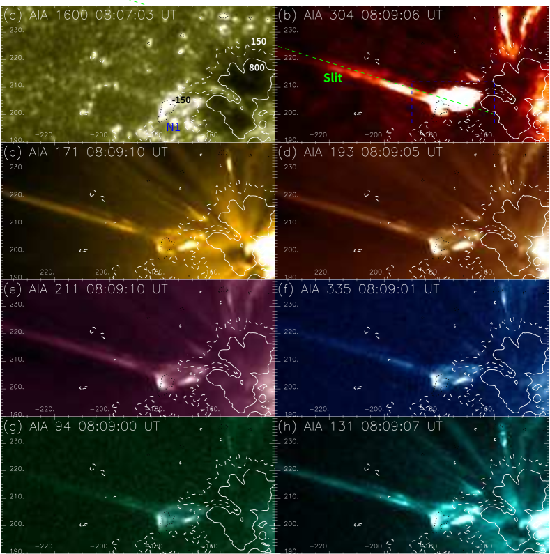
Figure 2: SDO/AIA observations of the sample jet formed at around 08:09 UT at 1600 Å (a), 304 Å (b), 171 Å (c), 193 Å (d), 211 Å (e), 335 Å (f), 94 Å (g) and 131 Å (h) passbands, respectively. Similar to the red solid, red dashed and green dashed contours in Fig. 1, the white solid, white dashed and black dashed contours here represent magnetic field levels of 800 G, 150 G and -150 G, respectively. The green dashed line in panel (b) indicate a 13^′′-wide slit for probing the axial motion of jets. The blue dashed box confines the region for calculating the normalized integrated intensity in Fig. 3(b). Coordinates are in units of arcsecond.

There are more than 10 jet eruptions originating from the emerging negative flux “N1” between 04:00-12:00 UT, observed by the SDO/AIA instrument. Most of the jets contain materials that can be found in all 7 AIA UV/EUV passbands (see the online movie M1, a supplement to Figure 2), suggesting their multi-thermal nature.

Among all these prominent jets, Figure 2 captures one at around 08:09 UT from the upper photosphere to the corona. Panel (a) shows the upper photospheric observation of the emerging flux and the nearby active region. Contours are similar to those in Figure 1 from the SDO/HMI LOS magnetic field data, with white solid, white dashed and black dashed curves indicating the LOS magnetic field strength at 800 G, 150 G and -150 G, respectively. The black dashed curve, representing the emerging negative flux “N1”, coincides with the brightness enhancement for the footpoint region of the jet, providing a direct evidence that the jet is initiated from the emerging flux.

Figures 2(b)-(h) show the UV/EUV observations of the jet at passbands of He II 304 Å (0.05 MK), Fe IX 171 Å (0.6 MK), Fe XII XXIV 193 Å (1.6 MK, 20 MK), Fe XIV 211 Å (2.0 MK), Fe XVI 335 Å (2.5 MK), Fe XVIII 94 Å (6.3 MK) and Fe VII XXI 131 Å (0.4 MK, 10 MK), respectively [Lemen et al., 2012]. Like most other jets in movie M1, this jet shows an “anemone” (“Reverse-Y” or “Eiffel-Tower”) shape (the elongated jet body and its loop-system base), which is common among such solar jets [e.g., Shibata et al., 2007] and can be well explained by existing jet models [e.g., Canfield et al., 1996]. Easily figured out from the UV/EUV observations, the jet-associated loops, appearing as brightness-enhanced arches, have one root region at the emerging negative flux “N1”. The other footpoint is at the edge of the main positive polarity, indicating that the jet should be triggered by reconnection between the emerging flux and ambient field lines from the positive polarities.

Along the 13^′′-wide slit, shown as the green dashed line in Figure 2(b), we construct the time-distance diagram in Figure 3(a). Cool and hot components of jet materials are shown in the tricolor channels. It turns out to be a “jet spectrum”, which shows the jet activities causing different intensity enhancements at different passbands along the given slit. Figure 3(b) depicts the normalized integrated intensity of 8 AIA passbands over the blue dashed box in Figure 2(b). Obviously, most jet eruptions found in panel (a) correspond to distinct intensity enhancements in all 8 utilized passbands at the emerging negative polarity “N1”. The region in gray shadow shows the time interval when there is a series of violent jet eruptions (referred to as “SJ” hereafter), during which jets are longer and more frequent.

4 Temporal Relationship between the Emerging Flux and Jets

To further investigate the temporal relationship between the footpoint-region emerging flux and the erupting jets, we visualize several characteristic physical parameters of the emerging flux in panel (c) to (e) in Figure 3, including the total negative LOS magnetic flux, the mean vertical current density, the mean current helicity, and the total photospheric free magnetic energy. The total negative LOS magnetic flux is obtained by integrating the negative data points within the region confined by the blue dashed box in Figure 1(e). The vertical current density is defined as:

$$\overline{J_{z}}\propto\frac{1}{N}\sum(\frac{\partial B_{y}}{\partial x}-\frac{\partial B_{x}}{\partial y}),$$ (1)

where $B_{x}$ and $B_{y}$ are the tangential components of the vector magnetic field obtained from the SHARPs data. The mean current helicity is derived from:

$$\overline{H_{c}}\propto\frac{1}{N}\sum B_{z}J_{z},$$ (2)

where $B_{z}$ is the vertical magnetic field and $J_{z}$ the vertical current density obtained from Eq. 1 [Leka and Barnes, 2003; Bobra et al., 2014]. To estimate the total photospheric free magnetic energy, we subtract the modulus of the potential magnetic field calculated by employing a Green Function method with unchanged vertical field component from the modulus of the observed magnetic field, followed by integrate the square of their difference over the blue dashed box in Figure 1(e) [e.g., Gary, 1996; Wang et al., 1996].

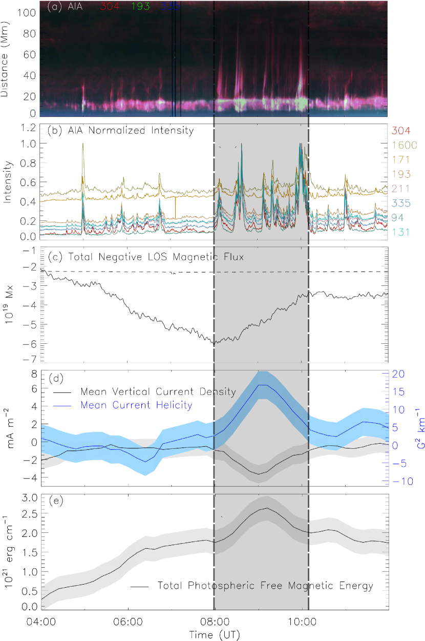
Figure 3: Panel (a): Time-distance diagram of AIA 304 Å (red), 193 Å (green) and 335 Å (blue) passbands along the slit in Fig. 2(b) from 04:00 UT to 12:00 UT. Panel (b): Normalized integrated intensities at 8 AIA passbands within the region confined by the blue dashed box in Fig. 2(b). Panel (c): Total negative magnetic flux (solid curve) integrating the HMI LOS magnetic field data within the blue dashed box Fig. 1(e), and the millionth of the total unsigned LOS magnetic flux for the entire active region (dashed curve). Panel (d): Mean vertical current density (black solid curve) and mean current helicity (blue solid curve) within the same region as panel (c). Panel (e): Total photospheric free magnetic energy (black solid curve) within the same region as panel (c). Shadows in panel (d) and (e) indicate corresponding errors.

The total emerging negative LOS magnetic flux peaks at $-6.0\times 10^{19}$ Mx at 08:00 UT, in the meantime the series of violent jet eruptions (“SJ”) begins (Fig. 3(c)). After 08:00 UT, the total emerging negative flux begins to decrease and stabilizes at $\sim-3.5\times 10^{19}$ Mx from 10:10 UT onwards, when is exactly the time “SJ” ends. The dashed curve in panel (c) stand for the millionth of the total unsigned LOS magnetic flux for the entire Active Region and it is found to be almost unchanged during the investigated period, which excludes the possibility that the temporal evolution of the total negative LOS flux in the emerging region is caused by the solar rotational effect.

The mean vertical current density (black solid curve in panel (d)), the mean current helicity (blue solid curve in panel (d)), and the total photospheric free magnetic energy (black solid curve in panel (e)) at the region of the emerging polarity “N1” show almost the same evolution with each other. We find a continuous increase in these three parameters before “SJ” begins, indicating the built-up of free energy and current helicity for the coming violent eruptions. After the eruption of several violent jets, part of the free energy is released and these parameters begin to decrease. Finally, these parameters stabilize from around 10:10 UT when “SJ” ends. After that, these three parameters all become non-zero but smaller than the peak, consistent with that there are still few jet eruptions with smaller length and longer time lag after the “SJ”.

5 Thermal and Kinetic Characteristics

In order to estimate the temperature and electron number density of jets and their corresponding footpoint regions, we employ the Differential Emission Measure (DEM) method described in Hannah and Kontar [2012] on the 6 AIA optically thin wavebands (171 Å, 193 Å, 211 Å, 335 Å, 94 Å and 131 Å). The method allows a fast recovery of the DEM from solar data and can help to estimate of uncertainties in the solution. The response functions of these 6 AIA passbands will result in a DEM/EM detection in a temperature range from 0.5 to 32 MK.

Figure 4 shows the DEM-Square-Root-Weighted (DEMSRW) temperature and electron number density distribution of two typical jets with one before and the other during the “SJ” as examples. The DEMSRW temperature is defined as follows:

$$\overline{T}=\frac{\sum\sqrt{DEM\cdot\Delta T}\ T}{\sum\sqrt{DEM\ \Delta T}},$$ (3)

considering that EM is proportional to the square of electron number density. The electron number density is obtained by $\sqrt{EM/h}$, where $EM$ is the total emission measure by integrating DEMs over the entire temperature range (0.5 - 32 MK), and $h$ the LOS depth which is 5 Mm, approximately the average width of these jets. The jet at 06:10 UT shows only one cool thread. Its most materials are at low-temperature ($<$ 2 MK) and low electron number density ($<$ $1.7\times 10^{9}$ cm^-3). On the other hand, the jet at 10:00 UT shows a hot thread and a relatively cool thread. The peak temperature and electron density of this jet are exceeding 16 MK and $7.0\times 10^{9}$ cm^-3, respectively.

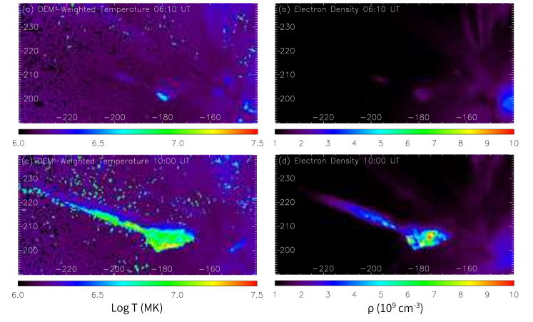
Figure 4: Panel (a) and (b): Distribution of the DEM-Square-Root-Weighted temperature and the electron number density at 06:10 UT. Panel (c) and (d): Distribution of the DEM-Square-Root-Weighted temperature and electron number density at 10:00 UT. Coordinates are in arcsecond.

Among these jets shown in Figure 3(a), only few of them are found not to be associated with the emerging flux “N1” based on a careful investigation of the AIA 1600 Å and HMI data. After excluding them, we estimate the physical properties of 11 jets (4 before, 4 during and 3 after the “SJ”) and list these parameters in Table 1. The second column lists the type of jets, with “Blowout” for jets with several threads and “standard” most-likely only one thread [e.g., Moore et al., 2010; Morton et al., 2012]. 3/4 before and 4/4 jets during the “SJ” are blowout type and 3/3 after the “SJ” are standard. To define the length of jets, we perform the Sobel edge enhancement [Sobel and Feldman, 1968] to the time-distance diagrams in AIA 304 Å, 171 Å, 193 Å, 211 Å and 131 Å passbands, in which all the investigated jets cause sufficient intensity enhancements. The yellow background in Figure  5(a) shows the original running-difference time-distance diagram in 193 Å passband as an example. Then we apply the Canny edge detection algorithm [Canny, 1986] to the Sobel-enhanced time-distance diagrams to define the edges of the jets (blue dots in Fig. 5(a)). The length of jets is then defined by the top of the blue dots along the trajectory of jets in the time-distance diagrams (red diamonds Fig. 5(a)), the corresponding error is determined by decreasing the brightness to half of the leading edge (green diamonds in Fig. 5(a)). Finally, we use the average value of all the lengths and errors obtained from the above five passbands for each jet. As we can see in Figure 5(a), the red diamonds always defines the leading edge with significant intensity variation and should be a lower limit of the real lengths of corresponding jets. The width of jets is obtained by the same method but of the original observations when jets grow to their maximum lengths (blue curves in Fig. 5(c) as an example), and the error of average width of each jet is the standard derivation of widths at different distances along the jet trajectory. Temperature and density are average values within the jet region also when it grows to its maximum length. Corresponding errors are estimated from the DEM method [Hannah and Kontar, 2012]. We find that even the peak temperatures and electron number densities are rather different for different types of jets as shown in Figure 4, the average values of them do not show much diversity. The average temperature and electron number density for all 11 jets range from 1.2$\pm$0.3 MK to 1.5$\pm$0.3 MK, and $0.7\pm 0.1\times 10^{9}$ cm^-3 to $1.1\pm 0.2\times 10^{9}$ cm^-3, respectively.

The mass of each jet is estimated by $\pi\rho L(\frac{d}{2})^{2}$, where $L$ is the length, $d$ the average width and $\rho$ the mass density. $\rho$ is set to be $\mu m_{0}n_{e}$, where $\mu$ is the mean molecular weight 0.58 for fully ionized coronal plasma, $m_{0}$ is the mass of proton and $n_{e}$ the estimated average electron number density of the jet. It turns out that the estimated mass of the jets ranges from $1.2\pm 0.4\times 10^{11}$ g to $38.1\pm 11.0\times 10^{11}$ g, with the maximum mass being more than 30 times larger than the minimum mass. We employ the equation $\frac{1}{2}mv^{2}$ to estimate the kinetic energy of each jet, where $m$ is the total mass and $v$ the projected axial speed. To obtain the projected axial speed of each jet, we apply the cross-correlation method developed by Tomczyk and McIntosh [2009] to different parts of the time-distance diagram in Figure 3(a). We cross-correlate the time series at each position along the slit with the time series at the midpoint of the slit. The peak of the cross-correlation function is then fitted with a parabola such that lag or lead time at each point along the slit is returned. We then fit the lag/lead times versus the distance along the slit with a straight line - the speed (and the associated error) of the propagating jet materials is the gradient of this line. At last a comparison between the speed and the gradient of the inclined features in the time-distance diagram is made to check the reliability of the results. The projected axial speed of all 11 jets turns out to be similar and has an average value of $383\pm 29$ km s^-1. Taking the common rotational motion along the axis for large-scale UV/EUV jets [e.g., Liu et al., 2015b, 2016] and the projection effect into account, we consider the kinetic energy of these jets estimated here to be most likely the lower limit of the true value. The kinetic energy estimated for all 11 jets ranges from $0.8\pm 0.3\times 10^{26}$ erg to $28.0\pm 9.1\times 10^{26}$ erg. Considering a fully ionized condition applicable the corona with thermal equilibrium and the value of Poisson constant $\gamma=5/3$, thermal energy of these jets is obtained by $3N\kappa_{p}T$, where $\kappa_{p}$ is the Boltzmann constant. $N=n_{e}V$ is the number of electrons the jet contains and $V$ is the volume of the jet. $T$ is the average DEMSRW temperature of the jet. Thermal energy of these jets has a range $0.6\pm 0.2\times 10^{26}$ erg to $22.0\pm 7.8\times 10^{26}$ erg. The ratios between the thermal and kinetic energy of jets are quite similar and range from 0.7 to 0.9, which is expected from the similar average temperature, average electron number density and axial speed for all these 11 jets.

Properties of the corresponding footpoint regions are also listed in the Table. The intensity enhancement (possibly a nano-flare) at the footpoint region during any of the studied jet events is not as significant as a typical flare, it is impossible to measure the strength of the brightening using GOES X-Ray observations or the flares’ thermodynamic spectrum based on the SDO/EVE observations [Wang et al., 2016]. An alternative option is to track the peak intensity of the footpoint region during each jet (which is usually several minutes before the jet gets to its maximum length) in the AIA 131 Å passband based on the consideration that during most flares the intensity change of 131 Å is always synchronous with that of the GOES X-Ray flux [e.g., Liu et al., 2015]. Similar as to define the length and width of jets, we perform the Sobel edge enhancement to the original AIA 131 Å images (Fig. 5(b) at 10:00 UT as an example) to make the footpoint region clearer (Fig. 5(c)). Blue curves in Figure 5(c) indicate the edges detected by the Canny algorithm and the red curve is drawn based on considering the combination of the Sobel edge-enhanced image and the detected Canny edges. Area and total intensity of each footpoint region then is obtained via integrating across the region within the red curve. A background at 03:27 UT when there is no apparent activities is subtracted from the obtained total intensity of each footpoint region to define the total intensity enhancement. The average temperature, average electron number density and thermal energy of each footpoint region are estimated in the same fashion with the corresponding jets.

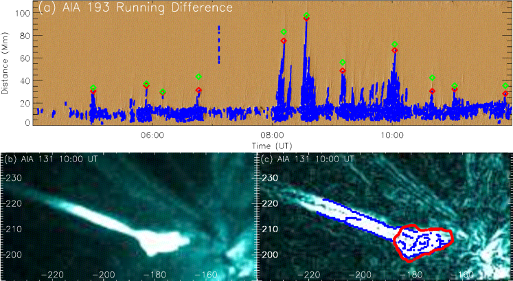
Figure 5: Panel (a): Running-difference time-distance diagram along the slit in Fig. 2(b) at AIA 193 Å passband. Blue dots mark the edges of jets given by the Canny edge detection method. Red diamonds mark the location of the jets’ leading edges and green diamonds the location when the brightness is decreased by 50%. Panel (b): AIA 131 Å observation of the jet and its footpoint at 10:00 UT. Panel (c): Edge enhanced image of panel (b) by the Sobel edge enhancement method. Blue curves indicate the edges detected by the Canny algorithm and the red curve is the drawn edge of the jet’s footpoint region. Coordinates are in units of arc second.

Table 1: Properties of 11 Prominent Jets and Their Footpoint Regions

	Jet								Footpoint Region
Time ($UT$)	Type	Length ($Mm$)	Width ($Mm$)	Temp ($MK$)	Density ($10^{9}$ $cm^{-3}$)	Mass ($10^{11}\ g$)	Kinetic Energy ($10^{26}\ erg$)	Thermal Energy ($10^{26}\ erg$)	Area ($Mm^{2}$)	TIE ($10^{2}\ DN$)	Temp ($MK$)	Density ($10^{9}$ $cm^{-3}$)	Thermal Energy ($10^{26}\ erg$)
05:00	Blowout	22.0$\pm$3.8	6.1$\pm$0.7	1.5$\pm$0.3	1.1$\pm$0.2	6.7$\pm$2.4	5.0$\pm$1.9	4.2$\pm$1.8	88.0$\pm$4.9	68.0$\pm$6.5	4.4$\pm$1.3	2.3$\pm$0.7	22.6$\pm$10.0
05:53	Blowout	26.8$\pm$4.3	6.5$\pm$0.4	1.5$\pm$0.3	1.0$\pm$0.2	9.0$\pm$2.7	6.6$\pm$2.2	5.8$\pm$2.2	99.0$\pm$6.5	63.6$\pm$3.6	3.1$\pm$0.8	2.0$\pm$0.5	16.2$\pm$6.1
06:10	Standard	18.7$\pm$3.2	2.9$\pm$0.2	1.2$\pm$0.3	1.0$\pm$0.2	1.2$\pm$0.4	0.8$\pm$0.3	0.6$\pm$0.2	47.0$\pm$3.8	5.7$\pm$0.5	2.5$\pm$0.7	1.7$\pm$0.4	2.3$\pm$0.9
06:46	Blowout	25.6$\pm$9.9	7.0$\pm$0.6	1.3$\pm$0.3	0.9$\pm$0.2	8.4$\pm$4.0	6.1$\pm$3.1	4.7$\pm$2.4	108.0$\pm$6.2	67.0$\pm$8.9	4.0$\pm$1.0	2.0$\pm$0.5	24.7$\pm$9.5
08:08	Blowout	63.0$\pm$16.2	4.5$\pm$0.4	1.4$\pm$0.3	0.8$\pm$0.2	7.9$\pm$2.9	5.8$\pm$2.3	4.6$\pm$2.0	126.5$\pm$5.5	65.5$\pm$3.3	3.5$\pm$1.0	2.1$\pm$0.6	17.4$\pm$7.0
08:35	Blowout	78.6$\pm$8.7	9.0$\pm$0.7	1.4$\pm$0.3	0.8$\pm$0.2	38.1$\pm$11.0	28.0$\pm$9.1	22.0$\pm$7.8	129.5$\pm$7.0	105.7$\pm$13.0	4.9$\pm$1.4	2.9$\pm$0.8	68.9$\pm$28.0
09:10	Blowout	45.1$\pm$4.6	4.8$\pm$0.6	1.3$\pm$0.3	0.8$\pm$0.2	6.5$\pm$2.1	4.8$\pm$1.7	3.7$\pm$1.4	104.0$\pm$5.3	49.8$\pm$6.8	3.7$\pm$1.0	2.2$\pm$0.6	17.1$\pm$7.1
10:00	Blowout	56.3$\pm$4.3	7.2$\pm$0.4	1.4$\pm$0.3	0.8$\pm$0.2	17.7$\pm$4.5	13.0$\pm$3.8	10.8$\pm$3.6	102.9$\pm$8.4	138.1$\pm$26.3	5.3$\pm$1.5	3.4$\pm$1.0	54.5$\pm$22.7
10:40	Standard	22.0$\pm$6.2	3.6$\pm$0.3	1.3$\pm$0.3	0.9$\pm$0.2	2.0$\pm$0.8	1.4$\pm$0.6	1.1$\pm$0.5	78.1$\pm$4.8	21.7$\pm$3.3	3.3$\pm$0.8	1.7$\pm$0.4	6.5$\pm$2.4
11:04	Standard	23.4$\pm$5.9	4.2$\pm$0.4	1.3$\pm$0.3	0.9$\pm$0.2	2.7$\pm$1.0	2.0$\pm$0.8	1.5$\pm$0.6	101.5$\pm$6.0	53.4$\pm$8.2	4.8$\pm$1.3	2.7$\pm$0.8	23.2$\pm$9.5
11:53	Standard	22.1$\pm$11.1	3.5$\pm$0.3	1.3$\pm$0.3	0.7$\pm$0.1	1.4$\pm$0.8	1.0$\pm$0.6	0.8$\pm$0.5	59.3$\pm$2.7	9.2$\pm$1.1	2.2$\pm$0.5	1.5$\pm$0.3	2.7$\pm$0.9

Note. TIE: footpoint region Total Intensity Enhancement

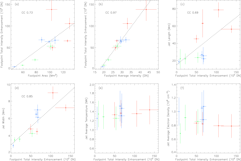
Figure 6: Panel (a)-(b): The footpoint-region total 131 Å intensity enhancement versus the footpoint-region area and footpoint-region average intensity, respectively. Panel (c)-(f): The jet length, average width, average DEMSRW temperature and average electron number density versus the total 131 Å intensity enhancement of corresponding footpoint region. Red symbols mark jets during the “SJ”, blue before and green after the “SJ”, with diamonds for the standard and asterisks for the blowout type, respectively. Black dashed lines are the linear fitting results.

6 Statistical Results

Figure 6(a) shows the area of jet footpoint regions versus the corresponding 131 Å total intensity enhancement, which presents a good positive relationship between them (CC $\approx$ 0.73). Red symbols mark jets during the “SJ”, blue before and green after it, with asterisks for blowout jets and diamonds for standard jets, respectively. Figure 6(b) illustrates that not only the area but also the intensity is positive related to the total intensity enhancement of the footpoint regions, suggesting that the intenser the reconnection which triggers the jet is, the larger the region it influences (the footpoint region of the jet) is. Most of the blowout jets have larger footpoint region and corresponding footpoint-region total intensity enhancement than standard jets, indicating that blowout jets should be triggered by intenser magnetic reconnection. Figure 6(c) to (f) show the jet length, average width, average temperature and average electron number density versus the total 131 Å intensity enhancement of corresponding footpoint regions, respectively. We can see from panels (c) and (d), the jet length and width show clear positive linear relationships with the footpoint-region total intensity enhancement, with a relatively high cross-correlation between them (CC $\approx$ 0.69 and 0.85). As the footpoint region total intensity enhancement is considered as a proxy of the intensity of the magnetic reconnection, we can then conclude that the magnetic reconnection which triggers the jet directly influences the length and width (thus the size) of the jet. And, from a comparison between the diamonds and asterisks, we can see blowout jets (especially those during the “SJ”) tend to be longer and wider than standard jets. However, as shown in panel (e) and (f), the cross-correlation coefficients of the jets’ average temperature and density with the footpoint region total intensity enhancement turn out to be very low. Shibata et al. [2007] suggest that the observed dominating temperature of X-ray, UV/EUV and spicule jets is mostly caused by the different heights where the jets are formed. For the recurrent homologous jets, here, they are most likely formed at similar heights with plasmas in similar temperature and density - resulting in the low correlation of these two properties with the intensity of the magnetic reconnection. It is believed that the axial speed of a jet is comparable with the local Alfvén speed where it is formed [Shibata et al., 1992], the similar axial speed of these jets again suggests that these jets should be formed at similar heights with similar magnetic field strength and plasma density.

The relationship between the jet mass and the footpoint-region total intensity enhancement is shown in Figure 7(a). They also show very high correlation (CC $\approx$ 0.89) with each other. Linear fit in log yields a slope of 0.96$\pm$0.16 ($\sim$1), showing the linear correlation between them. Considering the formula of the jet axial kinetic energy $\frac{1}{2}mv^{2}$ and the axial speed $v$ is similar for different jets, the jet axial kinetic energy should be also linearly positive related to the footpoint-region total intensity enhancement, which is proved in Figure 7(b). The index is the same for the jet thermal energy (Fig. 7(c)), as the jet thermal energy is proportional to $n_{e}Ld^{2}T$ and the jet average $T$ and average electron number density $n_{e}$ are not related to the footpoint-region total intensity enhancement (Fig. 6(e) and (f)). The similar linearly positive relationship also applies to that between the total intensity enhancement and the thermal energy of the footpoint regions.

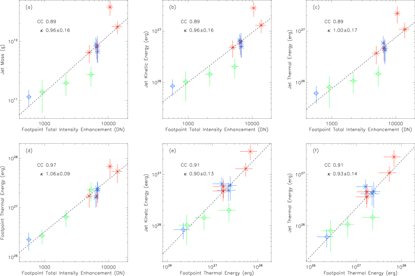
Figure 7: (a)-(d): The jet mass, axial kinetic energy, thermal energy and the footpoint-region thermal energy versus the total 131 Å intensity enhancement of corresponding footpoint region. (e)-(f): The jet kinetic energy and thermal energy versus the footpoint-region thermal energy. Same as Fig. 6, red symbols mark jets during the “SJ”, blue before and green after the “SJ”, with diamonds for the standard and asterisks for the blowout type, respectively. Black dashed lines are the linear fitting results.

The total free magnetic energy released during a jet event consists of at least the following four parts: footpoint region thermal energy (heating of post-flare loops etc.), non-thermal energy during the nano-flare [Testa et al., 2014], jet kinetic energy (axial and rotational) and jet thermal energy (heating of jet materials). We are unable to estimate the non-thermal energy released during these jet events and most of the rotational kinetic energy is not directly resulted from the reconnection [Liu et al., 2014]. Thus, we only investigate the relationship between the jet axial kinetic energy, the jet thermal energy and the footpoint-region thermal energy in Figure 7. From Figure 7(e), there is a very strong linearly positive relationship between the footpoint-region thermal energy and the jet axial kinetic energy (CC $\approx$ 0.91). The same linearly positive relationship also applies to that between the footpoint-region thermal energy and the jet thermal energy (CC $\approx$ 0.91, Fig. 7(f)). These results demonstrate a scenario that the more heating reconnection contributes to the footpoint region, the more heating and work reconnection contributes to the erupted jet material. This is consistent with the equipartition between kinetic and thermal energies during magnetic reconnections [e.g. Priest and Forbes, 2000]. Comparison between the diamonds and asterisks in all 6 panels in Figure 7 also reveals that blowout jets tend to have brighter footpoint regions, more mass, more kinetic/thermal energy than standard jets.

7 Summary and Conclusions

In this paper, we have performed a detailed analysis on 11 recurrent homologous jets observed by SDO/AIA and the related emerging (negative) flux observed by SDO/HMI from 03:00 UT to 12:00 UT on July 9th 2015. Let us summarize what we have learned from studying these jets and the evolution of the emerging flux as follows:

The (negative) flux “N1” emerges at 03:05 UT and only 6 minutes after that a jet erupts. After the emergence of “N1”, it becomes larger and larger, and more jets erupt. After 06:55 UT, the emerging flux seems to “calm down” for about 1 hour. At 08:04 UT, a jet with scale much larger than that of any before pops out from this emerging flux and it is only the beginning of a series of frequent eruptions (“SJ”). The “SJ” lasts for about 2 hours until 10:10 UT. After the “SJ”, there are still a few jets erupting from “N1”, but smaller in size.

Comparing all jets erupted from 04:00 UT to 12:00 UT, we find that all jets after the “SJ” are standard jets with only one thread, while most jets before and all jets during the “SJ” are blowout jets with several threads. Most of the jets show multi-thermal nature and can be observed in all 7 UV/EUV AIA passbands. Temporal investigation on the jets and the corresponding footpoint brightening shows that most jets have caused distinct intensity enhancements in all 8 utilized AIA passbands at footpoint regions. Comparing with the total (negative) LOS magnetic flux in the footpoint region, it is found that the “SJ” begins when the total (negative) flux peaks and starts to decrease. We further find that the mean vertical current density, the mean current helicity, and the total photospheric free magnetic energy, all continuously increase before and then decrease during the “SJ”. The above results suggest that with more available free magnetic energy, the eruptions of jets tend to be more violent, frequent and the blowout-like.

Among all the jets excluding those not related to the emerging flux, we investigate the properties of 11 jets and their corresponding footpoint regions. By utilizing a cross-correlation method, we find that all the jets have very similar projected axial speed around 383 km s^-1. Although the peak temperature and electron density of the blowout jets are significantly larger than those standard jets, the average values do not differ too much and are not related to the footpoint-region total 131 Å intensity enhancement, indicating that these jets should be formed by materials from similar origins.

The length and width of the jets show strong linearly positive relationships with the corresponding footpoint-region total intensity enhancement, indicating that a stronger footpoint-region reconnection induces a larger jet. With a cross-correlation coefficient of about 0.9, the mass of jets turns out to be linearly positive relative to the footpoint-region total intensity enhancement. The kinetic and thermal energy of jets also show the similar relationships with the footpoint-region total intensity enhancement, indicating that the intenser the footpoint region reconnection is, the more energy it injects into the jet. There are also very strong linearly positive relationships between the footpoint-region thermal energy and the kinetic/thermal energy of jets (CC $\approx$ 0.9), suggesting that the more heating reconnection contributes to the footpoint region plasma, the more heating and work reconnection contributes to the jet material. All the above results confirm the direct relationship between magnetic reconnection and jets, and validate the important role of magnetic reconnection in transporting large amount of free magnetic energy into jets.

However, as the number of homologous jets investigated in this paper is limited, it is hard to examine whether it is universal of the relationships found in this paper for different scales of jets in the Sun. Future work will include further statistical analysis of more homologous large-scale jets from different active regions, and combined studies of both large-scale and small-scale jets (spicules).