Dynamical structure factor of one-dimensional hard rods

Abstract

The zero-temperature dynamical structure factor $S(q,\omega)$ of one-dimensional hard rods is computed using state-of-the-art quantum Monte Carlo and analytic continuation techniques, complemented by a Bethe Ansatz analysis. As the density increases, $S(q,\omega)$ reveals a crossover from the Tonks-Girardeau gas to a quasi-solid regime, along which the low-energy properties are found in agreement with the nonlinear Luttinger liquid theory. Our quantitative estimate of $S(q,\omega)$ extends beyond the low-energy limit and confirms a theoretical prediction regarding the behavior of $S(q,\omega)$ at specific wavevectors $\mathcal{Q}_{n}=n2\pi/a$, where $a$ is the core radius, resulting from the interplay of the particle-hole boundaries of suitably rescaled ideal Fermi gases. We observe significant similarities between hard rods and one-dimensional ⁴He at high density, suggesting that the hard-rods model may provide an accurate description of dense one-dimensional liquids of quantum particles interacting through a strongly repulsive, finite-range potential.

I Introduction

One-dimensional (1D) quantum systems are subject to intense research, due to their theoretical and experimental peculiarities Giamarchi2004 ; Cazalilla2011 ; Imambekov2012 . On the theoretical side, the reduced dimensionality enhances quantum fluctuations and interaction, giving rise to unique phenomena like the nonexistence of Bose-Einstein condensation HMW ; Mermin1966 ; Coleman1973 ; Girardeau1960 ; Pitaevskii1993 and the breakdown of Fermi-liquid behavior Vignale2005 . On the experimental side, a 1D system is realized when a 3D system is loaded into an elongated optical trap or confined into a narrow channel, and the transverse motion is frozen to zero-point fluctuations.

Remarkably, several 1D many-body models of considerable conceptual and experimental relevance are exactly solvable Nagamiya1940 ; LiebLiniger1963 ; Lieb1963 ; Sutherland1971 ; Sutherland1971b ; Sutherland1988 , and provide a precious support for understanding static and dynamic properties of interacting 1D systems in suitable regimes expgen1 ; expgen2 ; expgen3 ; expdyn1 ; expdyn2 ; expdyn3 ; expdyn4 ; expsol1 ; expsol2 ; expfm1 ; expfm2 ; Fabbri2015 ; Bertaina2016 .

In particular, the behavior of 1D systems with a hard-core repulsive interaction, like ${}^{4}\mbox{He}$ or other gases adsorbed in carbon nanotubes Pearce2005 ; Mercedes2001 ; Mazzanti2008b ; Mazzanti2008a ; Bertaina2016 , can be understood making the assumption that particles behave like a gas of impenetrable segments or hard rods (HRs). Indeed, at high density, the principal effect of a short-range hard-core repulsive interaction is volume exclusion. Therefore, a reasonable approximation of the actual microscale behavior of the system can be obtained by taking into account the volume exclusion phenomenon only, neglecting all other details of the interaction: within this approach, the system is described as an assembly of HRs of a suitable length $a$.

The recognition that volume exclusion is the most important factor in analyzing short-range hard-core repulsive interactions in high-density classical systems dates back to the seminal work by van der Waals Waals1910 and Jeans Jeans1916 . It was later recognized Tonks1936 ; Hove1952 that the statistical mechanics of a system of classical HRs is exactly solvable. In 1940 Nagamiya proved Nagamiya1940 that also a system of quantum HRs is exactly solvable using the Bethe Ansatz technique, and imposing a special system of boundary conditions. Nagamiya’s treatment was later adapted by Sutherland Sutherland1971b to the more familiar periodic boundary conditions.

It is remarkable that local properties of the HR model are independent of the particles being bosons or fermions Girardeau1960 , since in 1D the hard core interaction creates nodes in bosonic wavefunctions which can be completely mapped to the nodes of fermionic wavefunctions. Only non-local properties differ, such as the momentum distribution Mazzanti2008b .

Even if the eigenfunctions and eigenvalues of the HR model can be determined exactly, so far the only systematic way to obtain a complete description of the ground-state correlation functions of the model has been the Variational Monte Carlo (VMC) method Mazzanti2008b ; Mazzanti2008a . Dynamical properties have also been addressed by using the variational Jastrow-Feenberg theory in Krotscheck1999 .

In the present work, we resort to state-of-the-art projective quantum Monte Carlo (QMC) Sarsa2000 ; Galli2003 ; Patate and analytic continuation Vitali2010 techniques to compute the dynamical structure factor, $S(q,\omega)$, of a single-component system of HRs. This analysis is supported by the Bethe Ansatz solution of the elementary excitations of the model, following Lieb1963 .

The dynamical structure factor characterizes the linear response of the system to an external field which weakly couples to the density. In the context of quantum liquids, it can be probed via inelastic neutron scattering Cowley1971 ; Beauvois2016 , while in the ultracold gases field it can be probed with Bragg scattering Ozeri2005 ; Fabbri2015 , also implemented via digital micromirror devices Ha2015 , or cavity-enhanced spontaneous emission Landig2015 .

While the low-energy properties of $S(q,\omega)$ are universal and can be described by the Tomonaga-Luttinger liquid (TLL) theory Tomonaga1950 ; Luttinger1963 ; Mattis1965 ; Haldane1983 ; Haldane1983b and its recent and remarkable generalization, called the nonlinear TLL theoryImambekov2009 ; Imambekov2012 , high-energy properties depend explicitly on the shape of the interaction potential, and lie in a regime beyond the reach of those theoretical approaches. Due to such limitation, we rely on QMC to estimate $S(q,\omega)$ for all momenta and energies.

The HR model, and its solution by Bethe Ansatz, is described in Section II. The methods used to compute the dynamical structure factor are reviewed in Section III. Results are presented and discussed in Section IV, and conclusions are drawn in the last Section V.

II The hard-rods model

Hard rods are the 1D counterpart of 3D hard spheres Mazzanti2008b ; Mazzanti2008a . The interparticle hard-rod potential is

$$V_{HR}(r)=\left\{\begin{array}[]{cc}\infty&|r|\leq a\\ 0&|r|>a\\ \end{array}\right.\quad,$$ (1)

where $a$ is the rod size. The Hamiltonian of a system of $N$ particles inside an interval $[0,L]$ of length $L$ with interparticle HR potential is

$$H=-\frac{\hbar^{2}}{2m}\,\sum_{i=1}^{N}\frac{\partial^{2}}{\partial r_{i}^{2}}+\sum_{i<j=1}^{N}V_{HR}(r_{i}-r_{j})\quad,$$ (2)

where $m$ is the mass of the particles, and $(r_{1}\dots r_{N})$ $\in\mathbb{R}^{N}$ their coordinates. The domain of the Hamiltonian operator (2) is the set of wavefunctions $\Psi(r_{1}\dots r_{N})\in\mathcal{L}^{2}(\mathbb{R}^{N})$ such that

$$\begin{split}&\Psi(r_{1}\dots r_{i}\dots r_{j}\dots r_{N})=\pm\,\Psi(r_{1}\dots r_{j}\dots r_{i}\dots r_{N})\,,\\ &\Psi(r_{1}\dots r_{i}\,+L\,\,\dots r_{N})=\phantom{\pm}\,\Psi(r_{1}\dots r_{i}\dots r_{N})\,,\\ &\Psi(r_{1}\dots r_{i}\dots r_{j}\dots r_{N})=0\,\,\,\,\mbox{if $|r_{i}-r_{j}|\leq a$}\,,\\ \end{split}$$ (3)

for any $i\neq j$. The first of the conditions (3) imposes Bose or Fermi symmetry, the second imposes periodic boundary conditions (PBC) and the third guarantees that $\langle\Psi|H|\Psi\rangle<\infty$. Thanks to the second equation in (3), we can concentrate on positions $(r_{1}\dots r_{N})\in\mathcal{C}=[0,L]^{N}$.

II.1 Solution by Bethe Ansatz

The solution of the HR Hamiltonian (2) was first addressed by Nagamiya Nagamiya1940 , relying on the Bethe Ansatz method Bethe1931 . The author substituted PBC (3) with slightly different boundary conditions, motivated by the study of particles arranged on a circle Nagamiya1940 . The solution of the HR Hamiltonian by Bethe Ansatz was subsequently addressed by Sutherland in Sutherland1971b , applying PBC.

In the present Section, we provide a detailed review of the solution of the HR model following the method of Refs.LiebLiniger1963 ; Lieb1963 , and a detailed description of its elementary excitations. This is a key ingredient that permits to characterize the singularities of $S(q,\omega)$ predicted by the nonlinear Luttinger liquid theory (Sec. II.4).

In order to solve the HR Hamiltonian (2), following Ref.Nagamiya1940 , let us concentrate on the sector $\mathcal{S}$ of the configuration space $\mathcal{C}$ where

$$\begin{split}&0<r_{1}<r_{2}-a\\ &r_{i-1}+a<r_{i}<r_{i+1}-a\quad i=2\dots N-1\\ &r_{N-1}+a<r_{N}<L-a\,,\\ \end{split}$$ (4)

which is related to all other sectors of the configuration space by a combination of permutations and translations of the particles, and eliminate the rod size $a$ by the transformation

$$x_{i}=r_{i}-(i-1)a\quad.$$ (5)

The rod coordinates $x_{i}$ lie in the set

$$0<x_{1}<x_{2}<\dots<x_{N}<L^{\prime}\quad,$$ (6)

where $L^{\prime}=L-Na$ is called the unexcluded volume. The HR Hamiltonian (2) then takes the form

$$H=-\frac{\hbar^{2}}{2m}\,\sum_{i=1}^{N}\frac{\partial^{2}}{\partial x_{i}^{2}}\quad,$$ (7)

and the third condition (3), imposing that particles collide with each other as impenetrable elastic rods, can be correspondingly expressed as

$$\tilde{\Psi}(x_{1}\dots x_{i}\dots x_{j}\dots x_{N})=0\quad\mbox{if $x_{i}=x_{j}$}\quad,$$ (8)

where we introduce the notation

$$\Psi(r_{1}\,r_{2}\dots r_{N})=\tilde{\Psi}(x_{1},\dots x_{N}),\quad(r_{1}\,r_{2}\dots r_{N})\in\mathcal{S}$$ (9)

to express $\Psi$ in terms of the rod coordinates. Eigenfunctions of (7) satisfying the condition (8) have the form Nagamiya1940

$$\tilde{\Psi}(x_{1}\dots x_{N})=\frac{1}{\sqrt{N!}}\,\mbox{det}\left(\frac{e^{ik_{i}x_{j}}}{\sqrt{L^{\prime}}}\right)\quad,$$ (10)

where $k_{1}\dots k_{N}$ are a set of quantum numbers called quasi-wavevectors, that will be identified later. The energy eigenvalue corresponding to (10) is ${E_{\{k\}}=\frac{\hbar^{2}}{2m}\,\sum_{i=1}^{N}k_{i}^{2}}$. Moreover, (10) is identically zero if and only if any two quasi-wavevectors coincide. The values of the quasi-wavevectors $k_{1}\dots k_{N}$ are fixed imposing PBC to the wavefunctions (10). Practically, imposing PBC means requiring that

$$\Psi(0\,r_{2}\dots r_{N})=\Psi(L\,r_{2}\dots r_{N})$$ (11)

for all $r_{2}\dots r_{N}$. Merging (10) and (11) one finds that PBC are satisfied if, for all quasi-wavevectors $k_{i}$, the following condition holds Sutherland1971b

$$(k_{i}-K)\,a=k_{i}(L-(N-1)a)-2\pi n_{i}+\xi^{B,F}(N)\quad,$$ (12)

where $i=1\dots N$, $K=\sum_{i=1}^{N}k_{i}$, $n_{i}\in\mathbb{Z}$ is an integer number, $\xi^{F}(N)=0$ and

$$\xi^{B}(N)=\left\{\begin{array}[]{cc}0&\mbox{for $N$ odd\,\,}\\ \pi&\mbox{for $N$ even}\\ \end{array}\right.\quad.$$ (13)

Equation (12) leads easily to

$$k_{i}=\frac{2\pi}{L^{\prime}}\,n_{i}-\frac{1}{L^{\prime}}\,\xi^{B,F}(N)-\frac{aK}{L^{\prime}}\quad.$$ (14)

Remarkably, even if the quasi-wavevectors $k_{i}$ are constructed with both $L$ and $L^{\prime}$, the total momentum $K$ is an integer multiple

$$K=\frac{2\pi}{L}\,\sum_{i=1}^{N}n_{i}-\frac{N\xi^{B,F}(N)}{L}$$ (15)

of $\frac{2\pi}{L}$. To summarize, the eigenfunctions of the HR Hamiltonian are in one-to-one correspondence with combinations of $N$ integer numbers without repetition.

II.2 Ground-state properties

For a system of $N$ Bose hard rods, the ground-state wavefunction is characterized by quasi-wavevectors

$$k_{i,GS}=\frac{2\pi}{L^{\prime}}\,n_{i,GS}\quad\quad n_{i,GS}=-n_{F}+(i-1)$$ (16)

symmetrically distributed around $0$, with ${n_{F}=(N-1)/2}$. The ground-state wavevector is naturally $K=0$. The ground-state energy reads Nagamiya1940 ; Mazzanti2008b :

$$\begin{split}E_{GS}&=\frac{\hbar^{2}}{2m}\left(\frac{2\pi}{L^{\prime}}\right)^{2}\frac{n_{F}(n_{F}+1)(2n_{F}+1)}{3}\end{split}$$ (17)

In the thermodynamic limit of large system size $N$ at constant linear density $\rho=N/L$, the ground-state energy per particle converges to

$$\begin{split}E_{\infty}=\lim_{N\to\infty}\frac{E_{GS}}{N}=\frac{\hbar^{2}k_{F}^{2}}{6m(1-\rho a)^{2}}\quad,\end{split}$$ (18)

where $k_{F}=\pi\rho$ is defined in analogy with the fermionic case. The reduced dimensionality is responsible for the fermionization of impenetrable Bose particles: the strong repulsion between particles mimics the Pauli exclusion principle Girardeau1960 . In particular, the limit $\rho a=0$ corresponds to the well-known Tonks-Girardeau gas, namely the hard-core limit of the Lieb-Liniger model LiebLiniger1963 , where all local properties are the same as for the ideal Fermi gas. At finite $\rho a$, we can think of HRs as evolving from the Tonks-Girardeau gas, in that the infinitely strong repulsive interaction is accompanied by an increasing volume exclusion. HRs are therefore a model for the super Tonks-Girardeau gas, which has been predicted and observed Astrakharchik2005 ; Batchelor2005 ; Tempfli2008 ; Haller2009 ; Panfil2013 as a highly excited and little compressible state of the attractive Lieb-Liniger Bose gas, in which no bound states are present.

In the case of hard rods, the eigenfunctions of both Bose and Fermi systems have the same functional form in the sector $\mathcal{S}$ of the configuration space; away from $\mathcal{S}$, they differ from each other only by a sign associated to a permutation of the particles Girardeau1960 . Therefore, the matrix elements of local operators like the density fluctuation operator

$${\rho}_{q}=\sum_{i=1}^{N}e^{-iq{r}_{i}}$$ (19)

are identical for Bose and Fermi particles. This, in particular, implies that the dynamical structure factor

$$S(q,\omega)=\int_{-\infty}^{\infty}dt\,\frac{e^{i\omega t}}{2\pi N}\,\langle\Psi|e^{itH/\hbar}{\rho}_{q}e^{-itH/\hbar}{\rho}_{-q}|\Psi\rangle$$ (20)

and the static structure factor

$$S(q)=\int_{0}^{\infty}d\omega S(q,\omega)=\frac{1}{N}\,\langle\Psi|{\rho}_{q}{\rho}_{-q}|\Psi\rangle$$ (21)

are independent of the statistics. Quite usefully for the purpose of QMC simulations in configuration space, the unnormalized bosonic ground-state wavefunction can be written in a Jastrow form for any $a$ Girardeau1960 ; Krotscheck1999 ; Mazzanti2008a :

$$\Psi_{GS}(r_{1}\cdots r_{N})=\prod_{i<j}|\sin{\pi(x_{j}-x_{i})/L}|\quad.$$ (22)

II.3 Elementary excitations

Figure 1: Pictorial representation of the Lieb-$I$ excitation with $p=6$ (top) and of the Lieb-$II$ excitation (middle) with $h=5$ for $N=7$ HRs. The Lieb-$II$ excitation with $h=1$ is called umklapp excitation (bottom).

In the previous Subsection II.2, we have recalled that the ground-state wavefunction of the HR system, once expressed in terms of the rod coordinates, has the functional form of a Fermi sea with renormalized coordinates and wavevectors $k_{i,GS}$, specified in terms of integer numbers $n_{i,GS}$. The excited states of the system are obtained creating single or multiple particle-hole pairs on top of this pseudo Fermi sea CastroNeto1994 . The simplest excitations, illustrated in Figure 1, consist in the creation of a single particle-hole pair

$$n_{i,PH}=n_{i,GS}+(p-n_{h,GS})\delta_{i,h}\quad,$$ (23)

where $h\in\{1\dots N\}$ is the index of the original quantum number to be modified (“hole”) and $p>n_{F}$ is the new integer quantum number of index $h$ (“particle”). Among single particle-hole excitations, a role of great importance in the interpretation of $S(q,\omega)$ is played by the following Lieb-I

$$n_{i,I}=n_{i,GS}+(p-n_{F})\,\delta_{i,N}$$ (24)

and Lieb-II

$$n_{i,II}=n_{i,GS}+(n_{F}+1-n_{h,GS})\,\delta_{i,h}$$ (25)

modes, which are reminiscent of the corresponding excitations of the Lieb-Liniger model Lieb1963 . As shown in Figure 1, in the Lieb-I excitation, a rod is taken from the Fermi level $h=N$ to some high-energy state associated to an integer $p>n_{F}$, while in the Lieb-II excitation a rod is taken from a low-energy state $h_{II}$ to just above the Fermi level $p=n_{F}+1$. In both cases, in view of the collective nature of the quasi-wavevectors $k_{i}$, the excitation of that rod provokes a recoil of all the other rods, according to Equations (14) and (15).

A simple calculation shows that the dispersion relation of the Lieb-I excitation is given by

$$E^{(N)}_{I}(q)=E_{I}(q)+\Delta E^{(N)}_{I}(q)$$ (26)

where $q\geq 0$ is the wavevector of the excitation. The dispersion relation $E_{I}(q)$ in the thermodynamic limit reads

$$\frac{E_{I}(q)}{E_{F}}=\frac{4}{K_{L}}\,\left(x+x^{2}\right)\quad,$$ (27)

In the previous equation $E_{F}=\frac{\hbar^{2}k_{F}^{2}}{2m}$, $x=\frac{q}{2k_{F}}$ and the physical meaning of the Luttinger parameter $K_{L}=(1-\rho a)^{2}$ will be elucidated in Section II.4. Size effects $\Delta E^{(N)}_{I}(q)$ have the form

$$\frac{\Delta E^{(N)}_{I}(q)}{E_{F}}=-\frac{2}{NK_{L}}\,x\,\left(1+(1-K_{L})x\right)$$ (28)

whenever $\xi^{B,F}(N)=0$. A similar calculation shows that the dispersion relation of the Lieb-II excitation is given by $E^{(N)}_{II}(q)=E_{II}(q)+\Delta E^{(N)}_{II}(q)$ with $0\leq q\leq 2k_{F}$ and

$$\begin{split}\frac{E_{II}(q)}{E_{F}}&=\frac{4}{K_{L}}\,\left(x-x^{2}\right)\quad,\\ \frac{\Delta E_{II}(q)}{E_{F}}&=\frac{E_{II}(q)}{N}+\frac{x^{2}}{N}\end{split}$$ (29)

Other relevant excitations are those producing supercurrent states Lieb1963 ; Vignale2005 ; Cherny2011

$$n_{i,SC}=n_{i,GS}+s\quad\quad s\in\mathbb{N}$$ (30)

with momenta $q=2sk_{F}$ and excitation energies $E_{sc}(q)=\frac{\hbar^{2}}{2m}\frac{q^{2}}{N}$ independent of the rod length $a$, and vanishing in the thermodynamic limit. Supercurrent states correspond to Galilean transformations of the ground state with velocities $v_{SC}=\frac{2\hbar k_{F}}{m}\,\frac{s}{N}$. The first supercurrent state, in particular, is also termed umklapp excitation Lieb1963 ; Vignale2005 ; Cherny2011 .

In the thermodynamic limit, the particle-hole excitations (23) span the region $\omega^{*}_{-}(q)\leq\omega\leq\omega^{*}_{+}(q)$ of the $(q,\omega)$ plane, where

$$\frac{\hbar\omega_{\pm}^{*}(q)}{E_{F}}=\frac{4}{K_{L}}\,\left|\frac{q}{2k_{F}}\pm\left(\frac{q}{2k_{F}}\right)^{2}\right|\quad.$$ (31)

The curves $\hbar\omega_{\pm}^{*}(q)$ have the same functional form of the ideal Fermi gas particle-hole boundaries $\hbar\omega_{\pm}(q)=|\hbar^{2}k_{F}q/m\pm\hbar^{2}q^{2}/2m|$, except for the substitution of the bare mass $m$ with $m^{*}=mK_{L}<m$, as we argued in Ref. Bertaina2016 .

The upper branch of this renormalized particle-hole continuum coincides with the Lieb-I mode. For $q\leq 2k_{F}$, its lower branch coincides with the Lieb-II mode and, for $q\geq 2k_{F}$, with the particle-hole excitations

$$n_{i,PH}=n_{i,GS}+1+(p-n_{N,GS}-1)\delta_{i,N}\quad,$$ (32)

resulting from the combination of the Lieb-I and the umklapp modes.

It is worth noticing that the Lieb-II dispersion relation constitutes the energy threshold for excitations for $0<q<2k_{F}$. Away from this basic region, the energy threshold in the thermodynamic limit can be obtained by a combination of inversions and shifts Imambekov2009 , and corresponds to a combination of a Lieb-II mode and multiple umklapp excitations. To summarize, the low-energy threshold is given by

$$\frac{\hbar\omega_{th}(q)}{E_{F}}=\frac{4}{K_{L}}\left(\frac{q^{*}_{n}}{2k_{F}}-\left(\frac{q^{*}_{n}}{2k_{F}}\right)^{2}\right)\quad,$$ (33)

where $2nk_{F}\leq q\leq 2(n+1)k_{F}$ and $q_{n}^{*}=q-2nk_{F}$. Finite size corrections are the same as in Eq. (29) Bertaina2016 .

Remarkably, (33) corresponds also to the dispersion relation of dark solitons of composite bosons in Yang-Gaudin gases of attractively interacting fermions in the deep molecular regime, even though in that case the molecular scattering length is negative (corresponding to a repulsive Lieb-Liniger molecular gas) Brand2016 .

II.4 Comparison with Luttinger liquid theories

The low-energy excitations of a broad class of interacting 1D systems are captured by the phenomenological TLL field theory Tomonaga1950 ; Luttinger1963 ; Mattis1965 ; Haldane1983 ; Haldane1983b ; Imambekov2012 . The TLL provides a universal description of interacting Fermi and Bose particles by introducing two fields, ${\phi}(x)$ and ${\theta}(x)$ representing the density and phase oscillations of the destruction operator ${\Psi}(x)\simeq\sqrt{\rho+\partial_{x}{\phi}(x)}e^{i{\theta}(x)}$, and a quadratic low-energy Hamiltonian describing the dynamics of those fields

$${H}_{LL}=\frac{\hbar}{2\pi}\int dx\left(cK_{L}\partial_{x}{\theta}(x)^{2}+\frac{c}{K_{L}}\partial_{x}{\phi}(x)^{2}\right)\quad.$$ (34)

For Galilean-invariant systems, the sound velocity $c$ is related to the positive Luttinger parameter $K_{L}$ through $c=\frac{v_{F}}{K_{L}}$. The quadratic nature of (34) allows for the calculation of correlation functions and thermodynamic properties in terms of $c$ and $K_{L}$. Within the TLL theory, in the low-momentum and low-energy regime $S(q,\omega)$ features collective phonon-like excitations $\omega_{LL}(q)=c|q|$ with sound velocity $c$.

The TLL theory has been recently extended Imambekov2009 ; Imambekov2012 beyond the low-energy limit, where the assumption of linear excitation spectrum $\omega_{LL}(q)$ is not sufficient for accurately predicting dynamic response functions. Assuming that, for any momentum $q$, $S(q,\omega)$ has support above a low-energy threshold $\omega_{th}(q)$ and interpreting excitations with momentum $q$ between $2nk_{F}$ and $2nk_{F}+2k_{F}$ as the creation of mobile holes of momentum $q_{n}^{*}=q-2nk_{F}$ coupled with the TLL Imambekov2009 ; Imambekov2012 , it is possible to show that for a broad class of Galilean-invariant systems $S(q,\omega)$ features a power-law singularity close to the low-energy threshold $\omega_{th}(q)$ with the following functional form:

$$S(q,\omega)=\theta\left(\omega-\omega_{th}(q_{n}^{*})\right)\,\left|\omega-\omega_{th}(q_{n}^{*})\right|^{-\mu_{n}(q)}\quad,$$ (35)

where the exponent

$$\begin{split}\mu_{n}(q)=1&-\frac{1}{2}\left((2n+1)\sqrt{K_{L}}+\frac{\delta_{+}(q_{n}^{*})+\delta_{-}(q_{n}^{*})}{2\pi}\right)^{2}\\ &-\frac{1}{2}\left(\frac{1}{\sqrt{K_{L}}}+\frac{\delta_{+}(q_{n}^{*})-\delta_{-}(q_{n}^{*})}{2\pi}\right)\\ \end{split}$$ (36)

is specified in terms of the phase shifts

$$\frac{\delta_{\pm}(q)}{2\pi}=\frac{\frac{1}{\sqrt{K_{L}}}\left(\frac{\hbar q}{m}+\frac{\partial\omega_{th}(q)}{\partial q}\right)\pm\sqrt{K_{L}}\left(\frac{v_{s}}{K_{L}}-\frac{1}{\pi}\frac{\partial\omega_{th}(q)}{\partial\rho}\right)}{2\left(\mp\frac{\partial\omega_{th}(q)}{\partial q}-v_{s}\right)}$$ (37)

The only phenomenological inputs required by the nonlinear TLL theory are the Luttinger parameter $K_{L}$ and the low-energy threshold $\omega_{th}(q)$, which in the case of hard rods are exactly known. Namely, we recall that the Luttinger parameter $K_{L}$ Haldane1983 ; Haldane1983b can be computed from the compressibility

$$\kappa_{S}^{-1}=\rho\,\frac{\partial}{\partial\rho}\left(\rho^{2}\,\frac{\partial E_{\infty}}{\partial\rho}\right)$$ (38)

through the formula $mK_{L}^{2}=\hbar^{2}\,k_{F}^{2}\,\rho\,\kappa_{S}$. The resulting exact expression, $K_{L}=(1-\rho a)^{2}$ Mazzanti2008a , provides a Luttinger parameter always smaller than $1$, and converging towards $0$ as the excluded volume $Na$ converges towards $L$. Notice that both Lieb-I and Lieb-II dispersions approach $q=0$ with slope equal to the sound velocity $c=\frac{v_{F}}{K_{L}}>v_{F}$. The low-energy threshold, Eq. (33), has been described in the previous Section.

Knowledge of these two quantities permits to compute the exponent $\mu_{n}(q)$ exactly from (36) and (37). We find Bertaina2016

$$\mu_{n}(q)=-2\left(\tilde{q}-n\right)\,\left(\tilde{q}-(n+1)\right)\quad,$$ (39)

with $\tilde{q}=\frac{qa}{2\pi}$. In Fig. 2 we show the power-law exponents for momenta $0<q<4k_{F}$ and different densities. Notice that the functional form of (39) is that of a sequence of parabola arcs, intersecting null values at the special momenta $\mathcal{Q}_{n}=n2\pi/a$, with integer $n<\rho a/(1-\rho a)$. Such momenta, even for larger $n$, have already been recognized to be special Mazzanti2008a , in that they admit the exact calculation of $S(\mathcal{Q}_{n})$ and $S(\mathcal{Q}_{n},\omega)$. Namely, for those special momenta, the HRs at density $\rho$ behave as an ideal Fermi gas with increased density $\rho^{\prime}=\rho/(1-\rho a)$.

It is worth pointing out that TLL theories have limits of applicability, and thus do not exhaust our understanding of 1D substances Caux2006 ; Fabbri2015 ; Meinert2015 . The investigation of dynamical properties like $S(q,\omega)$ beyond the limits of applicability of Luttinger liquid theories, where the Physics is non-universal, typically requires numerical calculations or QMC simulations Caux2006 ; DePalo2008 ; Bertaina2016 .

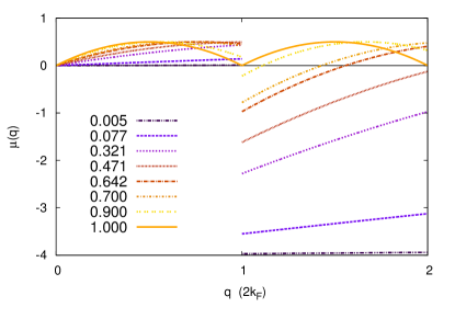
Figure 2: (color online) Nonlinear Luttinger theory exponents $\mu(q)$ for hard rods at the studied densities from $\rho a=0.077$ (blue solid line) to $\rho a=0.900$ (red solid line). Momenta are measured in units of $2k_{F}=2\pi\rho$. The $\rho a\to 1$ limit is also shown (solid line). Notice that the densities $\rho a\geq 0.5$ have a special wavevector $\mathcal{Q}_{1}$ between $2k_{F}$ and $4k_{F}$.

III Methods

In the present work, the zero-temperature dynamical structure factor of a system of Bose HRs is calculated using the exact Path Integral Ground State (PIGS) QMC method to compute imaginary-time correlation functions of the density fluctuation operator, and the state-of-the-art Genetic Inversion via Falsification of Theories (GIFT) analytic continuation method to extract the dynamical structure factor.

This approach, which we briefly review in this Section, has provided robust calculations of dynamical structure factors for several non-integrable systems like 1D, 2D and 3D He atoms Bertaina2016 ; Vitali2010 ; Nava2013 ; Arrigoni2013 and hard spheres Rota2013 .

The PIGS method is a projection technique in imaginary time that, starting from a trial wavefunction $\Psi_{T}(R)$, where $R=(r_{1}\dots r_{N})\in\mathcal{C}$ denotes a set of spatial coordinates of the $N$ particles, projects it onto the ground-state wavefunction $\Psi_{GS}(R)$ after evolution over a sufficiently long imaginary-time interval $\tau$ Sarsa2000 ; Galli2003 ; Patate . In typical situations, the functional form of $\Psi_{T}(R)$ is guessed combining physical intuition and mathematical arguments based on the theory of stochastic processes Holzmann2003 . $\Psi_{T}(R)$ is then specified by one or more free parameters, that are chosen using suitable optimization algorithms Kalos1986 ; Toulouse2007 ; Motta2015 .

In the case of HRs, knowledge of the exact ground-state wavefunction (22) makes the projection of a trial wavefunction $\Psi_{T}(R)$ approximating the ground state of the system unnecessary. However, the PIGS method can be used to give unbiased estimates of the density-density correlator

$$\begin{split}F(q,\tau)&=\langle\Psi_{GS}|e^{\tau H}{\rho}_{-q}\,e^{-\tau{H}}\,{\rho}_{q}|\Psi_{GS}\rangle=\\ &=\frac{\int dR_{M}dR_{0}\,p(R_{M},R_{0})\,\rho_{-q}(R_{M})\,\rho_{q}(R_{0})}{\int dR_{M}dR_{0}\,p(R_{M},R_{0})}\quad,\end{split}$$ (40)

with $p(R_{M},R_{0})=\Psi_{GS}(R_{M})G(R_{M},R_{0};\tau)\Psi_{GS}(R_{0})$ and $G(R_{M},R_{0};\tau)=\langle R_{M}|e^{-\tau{H}}|R_{0}\rangle$.

The propagator $G(R^{\prime},R;\tau)$ is in general not known, but suitable approximate expressions are available for small $\delta\tau=\tau/M$, where $M$ is a large integer number. Using one of these expressions in place of the exact propagator is the only approximation characterizing the calculations of the present work. The method is exact though, since this approximation affects the computed expectation values to an extent which is below their statistical uncertainty and such regime is always attainable by taking $\delta\tau$ sufficiently small. Then, the convolution formula permits to express $G(R_{M},R_{0};\tau)$ as

$$G(R_{M},R_{0};\tau)=\int dR_{M-1}\dots dR_{1}\prod_{i=0}^{M-1}G(R_{i+1},R_{i};\delta\tau)\,,$$ (41)

whence the PIGS estimator of $F(q,\tau)$ takes the form

$$\begin{split}F(q,\tau)=\frac{\int dX\,p(X)\,\rho_{-q}(R_{M})\,\rho_{q}(R_{0})}{\int dX\,p(X)}\,.\end{split}$$ (42)

In (42), $X=(R_{0}\dots R_{M})$ denotes a path in the configuration space $\mathcal{C}$ of the system, and

$$p(X)=\Psi_{GS}(R_{M})\prod_{i=0}^{M-1}G(R_{i+1},R_{i};\delta\tau)\Psi_{GS}(R_{0})$$ (43)

can be efficiently sampled using the Metropolis algorithm Metropolis1953 . In the present work, we have employed the pair-product approximation PP to express the propagator relative to a small time step $\delta\tau$ as

$$G(R,R^{\prime};\delta\tau)=\prod_{i=1}^{N}G_{0}(r_{i},r^{\prime}_{i};\delta\tau)\prod_{i<j}^{N}G_{\rm rel}(r_{ij},r^{\prime}_{ij};\delta\tau)\quad,$$ (44)

where $G_{0}$ is the free-particle propagator

$$G_{0}(r,r^{\prime};\delta\tau)=\frac{1}{\sqrt{2\pi\lambda\delta\tau}}e^{-(r-r^{\prime})^{2}/4\lambda\delta\tau}$$ (45)

with $\lambda=\hbar^{2}/2m$, and $G_{\rm rel}$ is obtained from the exactly known solution of the two-body scattering problem, similarly to a standard approach for hard spheres in 3D CaoBerne1992

$$G_{\rm rel}(r,r^{\prime};\delta\tau)=1-e^{-\frac{(r-a)(r^{\prime}-a)}{2\lambda\delta\tau}}\quad.$$ (46)

Moreover, in order to select an appropriately small $\delta\tau$, we have both checked the convergence of the static structure factor and the convergence of energy when the exact initial trial wavefunction is replaced with an approximate one Gordillo2012 .

The initial imaginary-time value of Eq. (40) is the static structure factor $F(q,0)=S(q)$. For finite values of $\tau$, $F(q,\tau)$ is instead related to $S(q,\omega)$ by the Laplace transform

$$F(q,\tau)=\int_{0}^{\infty}d\omega\,e^{-\tau\omega}\,S(q,\omega)\quad.$$ (47)

Equation (47) should be inverted in order to determine $S(q,\omega)$ from $F(q,\tau)$. However, it is well-known that such inverse problem is ill-posed, in the sense that many different trial dynamical structure factors, ranging from featureless to rich-in-structure distributions, have a forward Laplace transform which is compatible with the QMC results for $F(q,\tau)$: there is not enough information to find a unique solution of (47) Tarantola2006 ; MEM1 ; MEM2 ; MEM3 ; MEM4 ; Mishchenko2000 ; Vitali2010 . Different methodologies have been used to extract real-frequency response functions from imaginary-time correlators; in the present work, we rely on the Genetic Inversion via Falsification of Theories (GIFT) method Vitali2010 . The aim of GIFT is to collect a large collection of such dynamical structure factors in order to discern the presence of common features (e.g. support, peak positions, intensities and widths). The GIFT method has been applied to the study of liquid ${}^{4}\mbox{He}$ Overpress ; Anisotropic ; Bertaina2016 , 3D hard spheres Rota2013 , 2D Yukawa Bosons Molinelli2016 , liquid ${}^{3}\mbox{He}$ Nava2013 , 2D soft disks Saccani2011 ; Saccani2012 , the 2D Hubbard model Vitali2016 and 1D soft rods Teruzzi2016 , in all cases providing very accurate reconstructions of $S(q,\omega)$ or the single particle spectral function. Recently Bertaina2016 , we have shown that in 1D, when $\omega_{th}(q)$ is known, also the shape close to the frequency threshold can be approximately inferred. This is the reason why in subsection II.3 we insisted on the calculation of $\omega_{th}(q)$ for a finite system, which is a most useful quantity in our approach. Details of the GIFT method can be found in Vitali2010 ; Bertaina2016 . As in Bertaina2016 , we have used genetic operators which are able to better describe broad features typical of 1D systems. Moreover, the set of discrete frequencies of the model spectral functions used in the algorithm has been extended to non-equispaced frequencies, in order to better describe the regions where most of the weight accumulates.

$\rho a$	$K_{L}$
0.005	0.990
0.077	0.852
0.321	0.461
0.471	0.280
0.642	0.128
0.700	0.090
0.900	0.010

Table 1: Densities and values of $K_{L}$ studied in the present work.

IV Results

We computed $F(q,\tau)$ for systems of $N=50$ hard rods at densities $\rho a$ listed in Table 1, and wavevectors $q\leq 8k_{F}$. Before describing our results on the dynamical structure factor, we demonstrate the accuracy of our calculations by analyzing in detail finite-size effects on static properties which have already been studied in Ref. Mazzanti2008a .

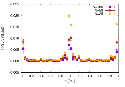
Figure 3: (color online) We quantify the finite-size effects on $S(q)$ at the representative density $\rho a=0.700$ computing the relative error $|S_{N}(q)-S_{\infty}(q)|/S_{\infty}(q)$, where $S_{\infty}(q)=\lim_{N\to\infty}S_{N}(q)$ is extrapolated. Away from the points $q=2k_{F},4k_{F}$, the relative error is below $1\%$ for $N=50$ particles.

IV.1 Assessment of accuracy

Results are affected by very weak finite-size effects, and thus are well representative of the thermodynamic limit. For example, (17) and (18) yield the following finite-size corrections to the ground-state energy

$$\frac{E_{GS}}{N}=E_{\infty}\left(1-\frac{1}{N^{2}}\right)$$ (48)

whence $\frac{E_{GS}}{50}=0.9996\,E_{\infty}$. To further assess the finite-size effects on our results, in Figure 3 we compute the static structure factor of $N=$ $50$, $100$ hard rods at $\rho a=0.700$ using the VMC method, which is an exact method when the exact (ground state) wave function is known, as in this case.

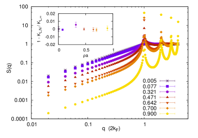
Figure 4: (color online) Static structure factor of $N=50$ rods at $\rho a=0.005$, $0.077$, $0.321$, $0.471$, $0.642$, $0.700$, $0.900$. Inset: relative error on the Luttinger parameter, computed from the low-momentum behavior of the static structure factor $S(q)\simeq K_{L}q/(2k_{F})$. In all cases, the relative error is below $1\%$.

At $q=2k_{F},4k_{F}$, the static structure factor displays peaks of diverging weight as predicted by the TLL theory Mazzanti2008a ; Astrakharchik2014 :

$$\begin{split}S(2mk_{F})&=S_{smooth}(2mk_{F})+S_{peak}(2mk_{F})=\\ &=S_{smooth}(2mk_{F})+C_{m}\,N^{1-2m^{2}K_{L}}\end{split}$$ (49)

Away from those points, the VMC estimates of the static structure factor are compatible with each other and with the extrapolation of $S(q)$ to the thermodynamic limit, within the error bars of the simulations, reflecting the weakness of finite-size effects. Moreover, in Figure 4 we show that static structure factors of $N=50$ rods permit to compute the Luttinger parameter $K_{L}$ without appreciable finite-size effects.

The same favorable behavior is exhibited by $F(q,\tau)$. In Figure 5, we show $F(q,\tau)$ for $N=50,100$ rods at the representative density $\rho a=0.700$. Away from $q=2k_{F}$ the two systems have statistically compatible $F(q,\tau)$, confirming the modest entity of finite-size effects.

IV.2 Dynamical structure factors

In Figure 6 we show the dynamical structure factor at densities ranging from $\rho a=0.005$ to $0.900$. At all the studied densities, for momentum $q<2k_{F}$, $S(q,\omega)$ has most of the spectral weight inside the particle-hole band $\omega^{*}_{-}(q)\leq\omega\leq\omega^{*}_{+}(q)$ spanned by single particle-hole excitations, Eq. (31). Contributions from multiple particle-hole excitations become relevant at high densities and momenta.

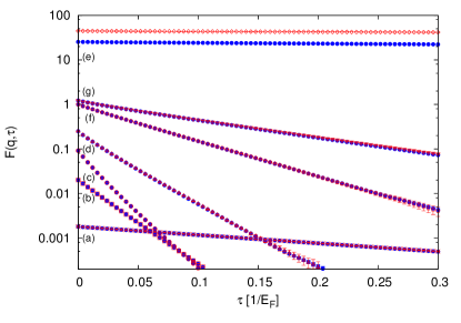
Figure 5: (color online) $F(q,\tau)$ of $N=50,100$ (blue circles, red open diamonds) rods at $\rho a=0.700$ for $\frac{q}{2k_{F}}=0.02$, $0.22$, $0.62$, $0.82$, $0.96$, $1.00$, $1.08$ (a to g). At $q=2k_{F}$ we observe strong finite-size effects, originating from the quasi-Bragg peaks in $S(q)$. Away from $q=2k_{F}$, in the relevant imaginary-time interval $\tau E_{F}\leq 0.3$ the two $F(q,\tau)$ are in satisfactory agreement.

At the lowest density, panel (a), the spectral weight is broadly distributed inside the particle-hole band, showing a behavior reminiscent of the Tonks-Girardeau model of impenetrable point-like bosons, to which the HR model reduces in the $\rho a\to 0$ limit.

The low momentum and energy behavior can be understood in the light of the nonlinear TLL theory: as illustrated in Figure 2, for momenta $q<2k_{F}$ it predicts a power-law behavior for $S(q,\omega)$, with an exponent (39) slightly larger than zero. This prediction is consistent with the spectrum in panel (a), showing a weak concentration of spectral weight close to the low-energy threshold for $q<2k_{F}$. For $q>2k_{F}$, the support of $S(q,\omega)$ departs from the low-energy threshold as it can be seen in panel (a), where the spectral weight remains concentrated inside the particle-hole band for all $q$. Correspondingly, for $2k_{F}<q<4k_{F}$, the nonlinear TLL predicts a large negative exponent, suggesting the absence of spectral weight in the proximity of the low-energy threshold.

A similar behavior is shown at density $\rho a=0.077$, panel (b), where the spectral weight concentrates more pronouncedly at the low-energy threshold for $q<2k_{F}$. This is again in agreement with the nonlinear TLL theory, predicting a larger negative exponent $\mu(q)$.

The dynamical structure factors in panels (a), (b) are also in qualitative agreement with numeric calculations for the super Tonks-Girardeau gas, for which $0.4\lesssim K_{L}<1$ Panfil2013 ; in fact we verified that the spectra shown in Ref. Panfil2013 manifest a low-energy support at positive energy which is compatible with Eq. (33), up to $\rho a\simeq 0.1$ (even though one should remark that a negative-frequency component is also present due to the excited nature of the super Tonks-Girardeau state).

The spectra in Figure 6 show that the Feynman approximation

$$\hbar\omega_{FA}(q)=\frac{\hbar^{2}q^{2}}{2mS(q)}$$ (50)

breaks down beyond $\frac{q}{2k_{F}}\simeq 0.1$. Interestingly, around $\frac{q}{2k_{F}}\simeq 0.1$ also the approximation of $\omega_{th}(q)$ with a linear function of $q$ ceases to be adequate. The simultaneous appearance of nonlinear terms in $\omega_{th}(q)$ and corrections to the Feynman approximation in $S(q,\omega)$ are in fact deeply related phenomena, as explained by the nonlinear TLL theory.

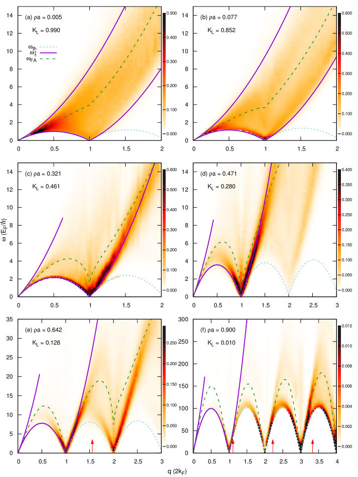
Figure 6: (color online) Color map of the dynamic structure factor, in units of $\hbar/E_{F}$, at $\rho a=0.005$, $0.077$, $0.321$, $0.471$, $0.642$, $0.900$ (left to right, top to bottom). Momenta are measured in units of $2k_{F}=2\pi\rho$ and energies in units of $E_{F}$. The low-energy threshold (blue dotted line), the branches $\omega_{\pm}^{*}(q)$ (purple solid lines) and the Feynman approximation for the excitation spectrum (green dashed line) are drawn for comparison. Panels (e), (f) also show the special wavevectors $\mathcal{Q}_{n}$ (red arrows).

When $K_{L}<1/2$, Eq. (49) indicates that a peak manifests in the static structure factor at $q=2k_{F}$. This change in behavior is also reflected in $S(q,\omega)$, as shown in panels (c), (d). The spectral weight concentrates close to the lower branch $\omega^{*}_{-}(q)$ of the particle-hole band, in a region of dense spectral weight that we call lower mode following Bertaina2016 , where a similar behavior was observed in 1D ⁴He at high density. In both HRs and ⁴He, above the lower mode stretches a high-energy structure gathering a smaller fraction of spectral weight. Such high-energy structure has a minimum at $q=2k_{F}$ close to the free-particle energy $E=4E_{F}$, and is symmetric around $q=2k_{F}$, (see panel (d) in Figure 6).

Panel (d) also shows that, as $K_{L}$ decreases below $1/2$, the support of $S(q,\omega)$ extends below $\omega^{*}_{-}(q)$ for $q>2k_{F}$, still remaining above $\omega_{th}(q)$. In the high-density regime $\rho a\geq 0.642$, such region of the momentum-energy plane hosts some of the most remarkable properties of $S(q,\omega)$ as it can be read from panel (e), where the shape of $S(q,\omega)$ changes considerably for $2k_{F}<q<4k_{F}$.

For $q<2.8k_{F}$, the spectral weight concentrates in a narrow region of the momentum-energy plane that gradually departs from the low-energy threshold. For $2.8k_{F}<q<3.6k_{F}$, $S(q,\omega)$ suddenly and considerably broadens and flattens. Finally, for $3.6k_{F}<q<4k_{F}$, the spectral weight again concentrates close to the low-energy threshold. This highly non-trivial behavior is in qualitative agreement with the nonlinear Luttinger liquid theory, predicting a negative exponent for $q<\mathcal{Q}_{1}$, where $\frac{\mathcal{Q}_{1}}{2k_{F}}=\frac{1}{a\rho}=1.558$. At $q=\mathcal{Q}_{1}$ the non-linear Luttinger liquid theory predicts a flat dynamical structure factor close to the low-energy threshold, in agreement with an exact prediction by F. Mazzanti et al. Mazzanti2008a and with our observations for the 1D HR system, but also for a 1D system of ⁴He atomsBertaina2016 . Beyond $\mathcal{Q}_{1}$ the non-linear Luttinger liquid theory predicts a positive exponent and we observe the spectral weight concentrating close to the low-energy threshold, as for $q<2k_{F}$. Notice that, although the condition for having quasi-Bragg peaks is $K_{L}<1/2$, the first special momentum with flat spectrum appears only for $\rho a>1/2$, namely $K_{L}<1/4$, since one must have $\mathcal{Q}_{1}=2\pi/a<4\pi\rho$.

It is well-known Mazzanti2008b ; Mazzanti2008a that, in the high-density regime $K_{L}\ll 1$, HRs show up a packing order leading to a quasi-solid phase, crystallization being prohibited by the reduced dimensionality and by the range of the interaction. The emergence of the quasi-solid phase is signaled by the peaks of the static structure factor, that approach the linear growth with the system size, peculiar prerogative of the Bragg peaks, only in the $\rho a\to 1$ limit.

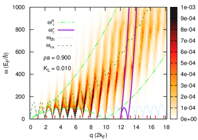
Figure 7: (color online) Color map of the dynamic structure factor at $\rho a=0.900$, on a much larger momentum and frequency scales than in Fig. 6(f). Units and reference curves are the same as in Fig. 6. The special wavevectors $\mathcal{Q}_{n}$ (red arrows) are shown by long (red) arrows. The role of both the HR renormalized particle-hole frequencies (solid curves) and of the reduced-volume ideal Fermi gas band (dot-dashed curves) are shown.

As far as $S(q,\omega)$ is concerned, the increase of the density transfers spectral weight to the low-energy threshold at wave vectors $q=2k_{F},4k_{F}$. We interpret this phenomenon as revealing that $S(q,\omega)$ is gradually approaching translational invariance $q\to q+2k_{F}$ in the variable $q$. This conjecture is corroborated by the observation that, as the density is further increased, the exponent $\mu_{n}(q)$ pointwise converges to the periodic function:

$$\mu_{n}(q)=-2\left(\frac{q}{2k_{F}}-n\right)\left(\frac{q}{2k_{F}}-(n+1)\right)$$ (51)

with $2nk_{F}\leq q\leq 2(n+1)k_{F}$ (illustrated in Figure 2). In this respect, it is interesting to observe panel (f) of Figure 6, showing the dynamical structure factor of HRs at $\rho a=0.900$. For $q<8k_{F}$, the spectral weight almost always concentrates around $\omega_{th}(q)$, except in the small ranges of wavevectors $2nk_{F}<q<\mathcal{Q}_{n}$. This makes $S(q,\omega)$ resemble the dispersion relation of longitudinal phonons of a monoatomic chain, in this range of momenta. However, the non-commensurability of $\mathcal{Q}_{1}$ with $2k_{F}$ renders the spectrum only quasi-periodic, a behavior which is more and more manifest at higher momenta. To analyze this intriguing regime in more detail, we have reconstructed the spectra at $\rho a=0.900$ up to $q=38k_{F}$. The results are shown in Fig. 7 and indicate a crucial role of the reduced-size ideal Fermi gas in drawing large-scale momentum and frequency boundaries for the HR spectrum. If we define the density $\rho^{\prime}=\rho/(1-\rho a)$, we observe that above $q=20k_{F}=2\pi\rho^{\prime}$, namely twice the Fermi momentum of the reduced-size IFG, the spectrum is never peaked along the low-energy HR threshold, however it presents a stripe structure, repeating the Lieb-I mode plus multiple umklapp excitations, and becoming again flat at momenta $\mathcal{Q}_{n}$. At the level of accuracy of our GIFT reconstructions, the stripes are bounded by the particle-hole band of the reduced-size IFG

$$\hbar\omega_{\pm}^{R}(q)=\frac{\hbar^{2}}{2m}\left|2\pi\rho^{\prime}q\pm q^{2}\right|\quad.$$ (52)

To corroborate this observation, we find that the special momenta $\mathcal{Q}_{n}$ also analytically correspond to the crossings of the lower reduced-size IFG boundary and the HR threshold (for $q<2\pi\rho^{\prime}$) or the HR repeated Lieb-I modes ($q>2\pi\rho^{\prime}$). It is tempting to conclude that the HR spectrum can be almost completely described by the synergy of two rescaled ideal Fermi gases: one with the same density, but renormalized mass $m^{*}=mK_{L}$, the other with the same mass, but increased density $\rho^{\prime}=\rho/K_{L}^{1/2}$.

Only in the unphysical $\rho a\to 1$ limit, therefore, $S(q,\omega)$ would attain the translational invariance observed for instance in half-filled Hubbard chains with strong on-site repulsion Pereira2012 ; Roux2013 .

Finally, in discussing Figure 6, we stressed in multiple occasions that low-energy properties of $S(q,\omega)$ are captured by the nonlinear TLL theory. Following the approach of Bertaina2016 , in Figures 8 and 9 we show that the agreement is quantitative, focusing on density $\rho a=0.700$ and two momenta close to $\mathcal{Q}_{1}$, representative of negative and positive power-law exponents, and fitting multiple spectral reconstructions with the functional form given by Eq. (35). The agreement with the analytical expression for the power-law exponent (39) is good, even though the accuracy is strongly dependent on the quality of the original $F(q,\tau)$ and it is particularly delicate to fit the spectra when the spectrum goes to zero close to the threshold.

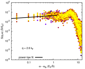
Figure 8: (color online) Power-law fit of reconstructed spectra for $\rho a=0.700$ and $q=2.6k_{F}$. The fitted exponent is $\mu=-0.18(3)$, which is compatible with the analytical prediction (51) that yields $\mu=-0.196$.

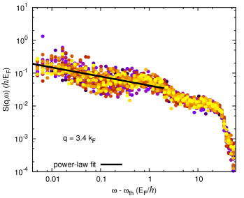
Figure 9: (color online) Power-law fit of reconstructed spectra for $\rho a=0.700$ and $q=3.4k_{F}$. The fitted exponent is $\mu=0.28(3)$, which is compatible with the analytical prediction (51) that yields $\mu=0.308$.

V Conclusions and Outlooks

We have computed the zero-temperature dynamical structure factor of one-dimensional hard rods by means of state-of-the-art QMC and analytic continuation techniques. By increasing the rod length, the dynamical structure factor reveals a transition from the Tonks-Girardeau gas, to a super Tonks-Girardeau regime and finally to a quasi-solid regime.

The low-energy properties of the dynamical structure factor are in qualitative agreement with the nonlinear LL theory. However, the methodology provides a quantitative estimation of the dynamical structure factor also in the high-energy regime, lying beyond the reach of LL theories. Our study reveals strong similarities between the dynamical structure factor of HRs and 1D ⁴He at linear densities $\rho\geq 0.150$ Å^-1 Bertaina2016 , extending to the high-energy regime (well above the low-energy threshold). In particular, both systems show a flat dynamical structure factor in correspondence of the wavevectors $\mathcal{Q}_{n}$, in agreement with a previous theoretical prediction Mazzanti2008a , and feature a high-energy structure overhanging the lower mode around the umklapp point $q=2k_{F}$. We have also unveiled a peculiar structure of the spectrum in the high-density and high-momentum regime, which can be described in terms of the particle-hole boundaries of two renormalized ideal Fermi gases.

At this point we want to remark that an intriguing feature of 1D ⁴He (and arguably of all 1D quantum liquids which admit a two-body bound state) is that its Luttinger parameter $K_{L}$ spans all positive values $0<K_{L}<\infty$ as the linear density is increased Bertaina2016 , not only the $K_{L}\leq 1$ regime, as in the case of HR or dipolar systems Citro2007 . This is due to the attractive tail of the interaction potential, which dominates at low density. Such feature has also to be contrasted to the repulsive Lieb-Liniger model, for which one obtains $1\leq K_{L}\leq\infty$ by tuning the interaction strength. Finally also the Calogero-Sutherland model reproduces all possible $K_{L}$, however by tuning interaction only Astrakharchik2006 .

We hope the present work will encourage further experimental research in 1D systems with volume exclusion effects, and theoretical investigation of the HR model. Our results may be relevant also for the linear response dynamics of resonant Rydberg gases in 1D configurations Petrosyan2013 . On the theoretical side, possible directions for further developments might be the alternative calculations of $S(q,\omega)$, based e.g. on the VMC evaluation of the matrix elements of $\rho_{q}$, and/or the calculation of finite-temperature equilibrium and dynamical properties.

- [1] T. Giamarchi, Quantum Physics in One Dimension, Oxford University Press (2004)
- [2] M.A. Cazalilla, R. Citro, T. Giamarchi, E. Orignac and M. Rigol, Rev. Mod. Phys. 83, 1405 (2011)
- [3] A. Imambekov, T. L. Schmidt and L. I. Glazman, Rev. Mod. Phys. 84, 1253 (2012)
- [4] P.C. Hohenberg, Phys. Rev. 158, 383 (1967)
- [5] N. D. Mermin and H. Wagner, Phys. Rev. Lett. 17, 1133 (1966)
- [6] S. Coleman, Commun. Math. Phys. 31, 259 (1973)
- [7] M. Girardeau, J. Math. Phys. 1, 516 (1960)
- [8] L. Pitaevskii and S. Stringari, Phys. Rev. B 47, 10915 (1993)
- [9] G. F. Giuliani and G. Vignale, Quantum Theory of the Electron Liquid, Cambridge University Press (2005)
- [10] T. Nagamiya, Proc. Phys. Math. Soc. Jpn. 22, 705 (1940)
- [11] E. H. Lieb and W. Liniger, Phys. Rev. 130, 1605 (1963)
- [12] E.H. Lieb, Phys. Rev. 130, 1616 (1963).
- [13] B. Sutherland, J. Math. Phys. 12, 251 (1971)
- [14] B. Sutherland Phys. Rev. A 4, 2019 (1971)
- [15] B. Sutherland, Phys. Rev. B 38, 6689 (1988)
- [16] P . Paredes, Nature 429, 277 (2004)
- [17] T. Kinoshita, T. Wenger and D. S. Weiss, Science 305, 1125 (2004)
- [18] E. Haller, M. Gustavss, M. J. Mark, J. G. Danzl, R. Hart, G. Pupillo and H. C. Negerl, Science 325, 1224 (2009)
- [19] H. P. Stimming, N. J. Mauser, J. Schmiedmayer and I. E. Mazets, Phys. Rev. Lett. 105, 015301 (2010)
- [20] M. Kuhnert, R. Geiger, T. Langen, M. Gring, B. Rauer, T. Kitagawa, E. Demler, D. Adu Smith and J. Schmiedmayer, Phys. Rev. Lett. 110, 090405 (2013)
- [21] S. Hofferberth, I. Lesanovsky, B. Fischer, T. Schumm and J. Schmiedmayer, Nature 449, 324 (2007)
- [22] T. Langen, R. Geiger, M. Kuhnert, B. Rauer and J. Schmiedmayer, Nature Physics 9, 640 (2013)
- [23] E. Witkowska, P. Deuar, M. Gajda and K. Rzazewski, Phys. Rev. Lett. 106, 135301 (2011)
- [24] T. Karpiuk, P. Deuar, P. Bienias, E. Witkowska, K. Pawlowski, M. Gajda, K. Rzazewski and M. Brewczyk, Phys. Rev. Lett. 109, 205302 (2012)
- [25] V. Guarrera, D. Muth, R. Labouvie, A. Vogler, G. Barontini, M. Fleischhauer and H. Ott, Phys. Rev. A 86, 021601 (2012)
- [26] J.P. Ronzheimer, M. Schreiber,S. Braun,S.S. Hodgman,S. Langer,I.P. McCulloch,F. Heidrich-Meisner,I. Bloch,U. Schneider, Phys. Rev. Lett. 110, 205301 (2013)
- [27] N. Fabbri, M. Panfil, D. Clément, L. Fallani, M. Inguscio, C. Fort, and J. S. Caux Phys. Rev. A 91, 043617 (2015)
- [28] G. Bertaina, M. Motta, M. Rossi, E. Vitali and D. E. Galli, Phys. Rev. Lett. 116, 135302 (2016)
- [29] J. V. Pearce, M. A. Adams, O. E. Vilches, M. R. Johnson and H. R. Glyde, Phys. Rev. Lett. 95, 185302 (2005)
- [30] M. Mercedes Calbi, M. W. Cole, S. M. Gatica, M. J. Bojan and G. Stan, Rev. Mod. Phys. 73, 857 (2001)
- [31] F. Mazzanti, G. E. Astrakharchik, J. Boronat and J. Casulleras, Phys. Rev. A 77, 043632 (2008)
- [32] F. Mazzanti, G. E. Astrakharchik, J. Boronat and J. Casulleras, Phys. Rev. Lett. 100, 020401 (2008)
- [33] J. D. Van der Waals, The equation of state for gases and liquids, Nobel Lectures in Physics 254 (1910)
- [34] J. H. Jeans, The Dynamical Theory of Gases, Cambridge University Press (1916)
- [35] L. Tonks, Phys. Rev. 50, 955 (1936)
- [36] B. R. A. Nijboer and L. Van Hove, Phys. Rev. 85, 777 (1952)
- [37] E. Krotscheck, M.D. Miller, and J. Wojdylo, Phys. Rev. B 60, 13028 (1999).
- [38] A. Sarsa, K. E. Schmidt, and W. R. Magro, J. Chem. Phys. 113, 1366 (2000)
- [39] D. E. Galli and L. Reatto, Mol. Phys. 101, 1697 (2003)
- [40] M. Rossi, M. Nava, L. Reatto, and D.E. Galli, J. Chem. Phys. 131, 154108 (2009)
- [41] E. Vitali, M. Rossi, L. Reatto and D. E. Galli, Phys. Rev. B 82, 174510 (2010)
- [42] R.A. Cowley and A.D.B. Woods, Can. J. Phys. 49, 177 (1971).
- [43] K. Beauvois, C.E. Campbell, J. Dawidowski, B. Fåk, H. Godfrin, E. Krotscheck, H.-J. Lauter, T. Lichtenegger, J. Ollivier, and A. Sultan, Phys. Rev. B 94, 024504 (2016).
- [44] R. Ozeri, N. Katz, J. Steinhauer, and N. Davidson, Rev. Mod. Phys. 77, 187 (2005).
- [45] L.-C. Ha, L.W. Clark, C.V. Parker, B.M. Anderson, and C. Chin, Phys. Rev. Lett. 114, 055301 (2015).
- [46] R. Landig, F. Brennecke, R. Mottl, T. Donner, and T. Esslinger, Nat. Commun. 6, (2015).
- [47] S. Tomonaga, Prog. Theor. Phys. 5, 544 (1950)
- [48] J. M. Luttinger, J. Math. Phys. 4, 1154 (1963)
- [49] D. C. Mattis and E. H. Lieb, J. Math. Phys. 6, 304 (1965)
- [50] F. D. M. Haldane, Phys. Rev. Lett. 47, 1840 (1981)
- [51] F. D. M. Haldane, Phys. Rev. Lett. 48, 569 (1982)
- [52] A. Imambekov and L. I. Glazman, Phys. Rev. Lett. 102, 126405 (2009)
- [53] H. Bethe, Zeit. Phys. 71, 205 (1931)
- [54] M. Panfil, J. De Nardis and J.-S. Caux, Phys. Rev. Lett. 110, 125302 (2013)
- [55] G. E. Astrakharchik, J. Boronat, J. Casulleras and S. Giorgini, Phys. Rev. Lett. 95, 190407 (2005)
- [56] M. T. Batchelor, M. Bortz, X. W. Guan and N. Oelkers, J. Stat. Mech. L10001 (2005)
- [57] E. Tempfli, S. Zöllner and P. Schmelcher, New J. Phys. 10, 103021 (2008)
- [58] E. Haller, M. Gustavsson, M.J. Mark, J.G. Danzl, R. Hart, G. Pupillo, and H.-C. Nägerl, Science 325, 1224 (2009).
- [59] A.H. Castro Neto, H.Q. Lin, Y.-H. Chen, and J.M.P. Carmelo, Phys. Rev. B 50, 14032 (1994).
- [60] A. Y. Cherny, J. S. Caux and J. Brand Frontiers of Physics 7, 54 (2012)
- [61] S.S. Shamailov and J. Brand, New J. Phys. 18, 75004 (2016)
- [62] J. S. Caux and P. Calabrese, Phys. Rev. A 74, 031605 (2006)
- [63] F. Meinert, M. Panfil, M. J. Mark, K. Lauber, J.-S. Caux and H.-C. Nägerl, Phys. Rev. Lett. 115, 085301 (2015)
- [64] S. De Palo, E. Orignac, R. Citro, and M.L. Chiofalo, Phys. Rev. B 77, 212101 (2008)
- [65] M. Nava, D.E. Galli, S. Moroni and E. Vitali, Phys. Rev. B 87, 144506 (2013)
- [66] F. Arrigoni, E. Vitali, D. E. Galli and L. Reatto, Low Temp. Phys. 39, 793 (2013)
- [67] R. Rota, F. Tramonto, D.E. Galli and S. Giorgini, Phys. Rev. B 88, 214505 (2013)
- [68] M. Holzmann, D. M. Ceperley, C. Pierleoni and K. Esler, Phys. Rev. E 68, 046707 (2003)
- [69] M. H. Kalos and P. A. Whitlock Quantum Monte Carlo, in Monte Carlo Methods, Wiley (1986)
- [70] J. Toulouse and C. J. Umrigar, J. Chem. Phys. 126, 084102 (2007)
- [71] M. Motta, G. Bertaina, D. E. Galli and E. Vitali, Comp. Phys. Comm. 190, 62 (2015)
- [72] N. Metropolis, A. W. Rosenbluth, M. N. Rosenbluth, A. H. Teller and E. Teller, J. Chem. Phys. 21 1087 (1953)
- [73] D. Ceperley, Rev. Mod. Phys. 67, 279 (1995)
- [74] J. Cao and B.J. Berne, J. Chem. Phys. 97, 2382 (1992)
- [75] F. De Soto and M.C. Gordillo, Phys. Rev. A 85, 013607 (2012)
- [76] A. Tarantola, Nature Physics 2, 492 (2006)
- [77] R. N. Silver, J.E. Gubernatis, D. S. Sivia and M. Jarrell, Phys. Rev. Lett. 65, 496 (1990)
- [78] M. Jarrell and J.E. Gubernatis, Phys. Rep. 269, 133 (1996)
- [79] M. Boninsegni, and D.M. Ceperley, J. Low Temp. Phys. 104, 339 (1996)
- [80] A. Roggero, F. Pederiva and G. Orlandini Phys. Rev. B 88, 094302 (2013)
- [81] A.S. Mishchenko, N.V. Prokof’ev, A. Sakamoto, and B.V. Svistunov, Phys. Rev. B 62, 6317 (2000).
- [82] M. Rossi, E. Vitali, L. Reatto and D.E. Galli, Phys. Rev. B 85, 014525 (2012)
- [83] M. Nava, D.E. Galli, M.W. Cole, L. Reatto, J. Low Temp. Phys. 171, 699 (2013)
- [84] S. Molinelli, D. E. Galli , L. Reatto and M. Motta, J. Low Temp. Phys. DOI: 10.1007/s10909-016-1628-3 (2016)
- [85] S. Saccani, S. Moroni, E. Vitali, and M. Boninsegni, Mol. Phys. 109, 2807 (2011).
- [86] S. Saccani, S. Moroni, and M. Boninsegni, Phys. Rev. Lett. 108, 175301 (2012).
- [87] E. Vitali, H. Shi, M. Qin, and S. Zhang, Phys. Rev. B 94, 085140 (2016).
- [88] M. Teruzzi, D.E. Galli, and G. Bertaina, arXiv:1607.05308 (2016).
- [89] G. E. Astrakharchik and J. Boronat, Phys. Rev. B 90, 235439 (2014)
- [90] G. Roux, A. Minguzzi and T. Roscilde, New J. Phys. 15, 055003 (2013)
- [91] R. G. Pereira, K. Penc, S. R. White, P. D. Sacramento and J. M. P. Carmelo, Phys. Rev. B 85, 165132 (2012)
- [92] R. Citro, E. Orignac, S. De Palo, and M.L. Chiofalo, Phys. Rev. A 75, 051602 (2007)
- [93] G.E. Astrakharchik, D.M. Gangardt, Y.E. Lozovik, and I.A. Sorokin, Phys. Rev. E 74, 021105 (2006)
- [94] D. Petrosyan, M. Höning, and M. Fleischhauer, Phys. Rev. A 87, 053414 (2013)