New $T_{\rm eff}$ and [Fe/H] spectroscopic calibration for FGK dwarfs and GK giants

Abstract

Context. The ever-growing number of large spectroscopic survey programs has increased the importance of fast and reliable methods with which to determine precise stellar parameters. Some of these methods are highly dependent on correct spectroscopic calibrations.

Aims. The goal of this work is to obtain a new spectroscopic calibration for a fast estimate of $T_{\rm eff}$ and [Fe/H] for a wide range of stellar spectral types.

Methods. We used spectra from a joint sample of 708 stars, compiled from 451 FGK dwarfs and 257 GK-giant stars. We used homogeneously determined spectroscopic stellar parameters to derive temperature calibrations using a set of selected EW line-ratios, and [Fe/H] calibrations using a set of selected Fe i lines.

Results. We have derived 322 EW line-ratios and 100 Fe i lines that can be used to compute $T_{\rm eff}$ and [Fe/H], respectively. We show that these calibrations are effective for FGK dwarfs and GK-giant stars in the following ranges: $4500\ K<\mbox{$T_{\rm eff}$ }<6500\ K$ , $2.5<\log g<4.9\ dex$, and $-0.8<[Fe/H]<0.5\ dex$. The new calibration has a standard deviation of 74 K for $T_{\rm eff}$ and $0.07\ dex$ for [Fe/H]. We use four independent samples of stars to test and verify the new calibration, a sample of 56 giant stars, a sample composed of Gaia FGK benchmark stars, a sample of 36 GK-giant stars of the DR1 of the Gaia-ESO survey, and a sample of 582 FGK-dwarf stars. We also provide a new computer code, GeTCal, for automatically producing new calibration files based on any new sample of stars.

1 Introduction

The derivation of accurate and precise stellar parameters has become a fundamental aspect of astrophysical studies. Parameters such as stellar mass, radius, and age are tremendously important, but very difficult to measure directly.

Stellar parameters are important for a diverse range of astrophysical studies: from characterization of planet-host stars to Galactic population studies (Edvardsson et al. (1993); Fischer et al. (1993); Casagrande et al. (2010); Huber et al. (2012); Mortier et al. (2013); Bensby et al. (2014); Chaplin et al. (2014), to name a few). The determination of mass, radius, and age requires a knowledge of stellar atmospheric parameters, such as effective temperature ($T_{\rm eff}$ ), surface gravity ($\log g$), metallicity ([Fe/H]), and microturbulence($v_{mic}$), which can be obtained mainly by spectroscopic or photometric methods (e.g. Sousa et al. (2008); Casagrande et al. (2010); Tsantaki et al. (2013)).

Large-survey observational programs such as GES (Gilmore et al., 2012), GALAH (Bland-Hawthorn et al., 2014), and RAVE (Steinmetz et al., 2006) are quickly becoming the new paradigm of stellar observations and characterization. Given the volume of data involved, the success of these programs relies on the existence of methods that rapidly ascertain stellar parameters for a diverse range of stellar spectral types. Such methods cover a broad range of evolutionary stages from main-sequence dwarf stars to post-main-sequence giants and all the intermediate stage stars. Since it is difficult to effectively cover such a diversity of evolutionary stages in a uniform way, broad-range methods are rare. These stars can be studied by methods like the line-strength ratios to obtain $T_{\rm eff}$ (Gray, 1996, 2005; Kovtyukh et al., 2003), and equivalent widths (EWs) of Fe i to derive [Fe/H] (Sousa et al., 2012). One of the most important steps in building these methods is to obtain an empirical calibration.

One of the spectroscopic methods that can be used to determine spectral parameters is the ARES+MOOG method. This method computes stellar atmospheric parameters based on the use of two codes: ARES and MOOG. The ARES code is an automated tool for obtaining the EWs of a spectrum based on an initial line list, and also weights parameters like the signal-to-noise ratio (S/N) (Sousa et al., 2007, 2015). MOOG is able to perform a variety of spectral line analyses and synthesis computations under local thermodynamic equilibrium (LTE) conditions (Sneden, 1973). In the ARES+MOOG method, MOOG is used to measure individual line abundances and is combined with a minimization algorithm based on the simplex method to derive the parameters of the stellar atmosphere that best fits the measured EWs. For a more detailed description of this method see Sousa (2014).

Sousa et al. (2012) presented an automated tool, TMCalc, with which $T_{\rm eff}$ and [Fe/H] can be obtained extremely fast using measurements of EWs of spectral lines. It is based on EW line-ratios and on the EWs of Fe i lines. The accuracy and precision of the results produced by TMCalc are mainly limited by the $T_{\rm eff}$ and [Fe/H] calibrations, the EW measurements, and the (S/N) of the stellar spectra (Sousa et al., 2012). The goal of our work is to produce a new calibration that is compatible with a broader regime of stellar evolutionary stages.

The main difference between using TMCalc and the ARES+MOOG method is that with TMCalc we obtain $T_{\rm eff}$ and [Fe/H] by a simple application of EW line ratios, while in ARES+MOOG a minimization procedure is performed to obtain the stellar atmospheric parameters. TMCalc is therefore less accurate, but it is computationally more efficient.

The paper is organized as follows: in Sect. 2 we present the stellar samples we used and the updated parameters. In Sect. 3 we explain the different steps and assumptions for $T_{\rm eff}$ and [Fe/H] calibrations, and we present an automatic calibration tool: GeTCal. In Sect. 4 we compare the new calibration with the pre-existing one, show the parameters obtained for two independent samples, and make some considerations on the effect that a poor $T_{\rm eff}$ determination may have on [Fe/H] calculations. Finally, in Sect. 5 we summarize our results.

2 Stellar samples

Our work was performed using six distinct stellar samples: two samples were used for calibration and four other samples were used for independent testing of the new calibration. A summary of each sample can be found in Table 1, where we provide the number of stars, (S/N), spectral classification, and intervals in $T_{\rm eff}$ , $\log g$, $v_{mic}$ , and [Fe/H] for each sample.

All samples parameters have been consistently determined homogeneously with ARES+MOOG.

We measured the EWs for all stars in the six samples with the initial line list of Sousa et al. (2010) to obtain homogeneous and comprehensive measurements and taking into consideration the different (S/N) of each spectrum.

ARES performs a local normalization before measuring the EWs. The errors on the measured EWs depend on the different (S/N), and line-blends are taken into account since ARES performs multi-line fits (Sousa et al., 2007). Although the new version of ARES reports errors on the EWs (Sousa et al., 2015), this work made use of the previous version.

2.1 Calibration samples

To obtain the new calibration, we used two samples:

• The sample of well-studied 451 FGK-dwarf stars described in Sousa et al. (2008) that was revised in Tsantaki et al. (2013), hereafter the So08 sample.

• The sample of 257 giant stars from Alves et al. (2015), hereafter the Al15 sample.

The So08 sample is composed of high-quality spectra of 451 FGK-dwarf stars with well-determined parameters (Sousa et al., 2008; Tsantaki et al., 2013). These stars have been analysed using HARPS high-resolution spectral data with a resolution $R\sim 110000$ and an (S/N) ranging from $\sim 70$ to $\sim 2000$. The parameters for this sample were revised in Tsantaki et al. (2013) to address an overestimation of $T_{\rm eff}$ for stars in the low-temperature regime, $\mbox{$T_{\rm eff}$ }<5200\ K$. In the remainder of this work, when we refer to the So08 sample, we refer to the corrected sample.

The Al15 sample is composed of high-resolution spectra obtained with the UVES spectrograph for 257 GK-giant stars. The spectra have resolutions of $\sim 110000$ with an (S/N) of $\sim$ 150. The parameters for these stars have been determined by Alves et al. (2015) using the same standard analysis of ARES+MOOG as in this work.

A joint sample, composed of the So08 and Al15 samples, was used as the calibration sample for our study, hereafter the joint sample.

Table 1: Summary of the stellar samples.

Sample	stars	stars_used	(S/N)	Spec type	$T_{\rm eff}$	$\log g$	$v_{mic}$	[Fe/H]
					($K$)	($dex$)	($kms^{-1}$)	($dex$)
So08	$451$	$451$	$[70,2000]$	FGK	$[4400,6431]$	$[3.60,4.82]$	$[0,2.1]$	$[-0.83,0.36]$
Al15	$257$	$257$	$\sim 150$	GK	$[4724,5766]$	$[2.37,3.92]$	$[1.08,4.28]$	$[-0.75,0.27]$
Sa09	$56$	$44$	$\sim 200$	GK	$[4157,6020]$	$[1.15,4.82]$	$[0.86,2.26]$	$[0,0.32]$
Gaia	$34$	$18$	$[200,400]$	FGK	$[3472,6635]$	$[0.51,4.67]$	$[0.89,1.92]$	$[-2.64,0.35]$
GES	$36$	$36$	$\sim 100$	GK	$[4753,5289]$	$[2.50,3.86]$	$[1.17,4.06]$	$[-0.51,0.25]$
So11	$582$	$582$	$[100,200]$	FGK	$[4487,7212]$	$[3.61,4.96]$	$[0,2.87]$	$[-1.14,0.55]$

2.2 Validation samples

To test the new calibration, we used four distinct and independent samples:

• The sample of 44 giant stars from Santos et al. (2009), hereafter the Sa09 sample.

• A sample of 18 benchmark stars of the Gaia survey, hereafter the Gaia sample (Jofré et al., 2014; Heiter et al., 2015).

• A subsample of 36 GK-giant stars from the Gaia-ESO survey DR1 with $\log g<3.9$, hereafter the GES sample.

• A sample of 582 FGK-dwarf stars from Sousa et al. (2011) with with well-determined parameters, hereafter the So11 sample.

The histograms with the distribution of $T_{\rm eff}$ , $\log g$, and [Fe/H] of the validation samples is shown in Fig. 1.

The Sa09 sample of 56 giant stars has been observed using the UVES spectrograph, with a spectral resolution of between $R\sim 50000$ and $\sim 100000$ and an (S/N) of $\sim 200$. The parameters used for the Sa09 sample were rederived in this work using the ARES+MOOG method. Using the applicability criteria, which we discuss in detail in Sect. 4.1, this sample was reduced to 44 stars within our applicability limits.

The Gaia sample is composed of the 34 FGK benchmark stars with well-determined values (Jofré et al., 2014). Of these, we used a sub-sample of 28 stars since the remaining six stars were M dwarfs and therefore unsuitable for EW automatic measurements. A final selection was applied to have only stars that fulfilled our applicability criteria, leading to 18 benchmark stars. The spectra have a high resolution (from HARPS and NARVAL spectrographs) and high (S/N), with values ranging from $\sim 200$ to $\sim 400$. The parameters of this sample were obtained by combining the EW methods of several work groups in the Gaia-ESO survey (Jofré et al., 2014; Heiter et al., 2015).

The GES subsample is composed of 36 GK-giant stars. The data used were taken from the Gaia-ESO survey DR1 spectra. The parameters for this sample have been derived using ARES+MOOG within the Porto/CAUP node in GES. The stars in these sample were observed for GES with the UVES spectrograph in the 580 nm setup. The (S/N) of the spectra was $\sim 100$.

The So11 sample is composed of 582 FGK-dwarf stars. The data used were taken from the So11 spectra. The (S/N) of the spectra ranged from $\sim 100$ to $\sim 200$. The EWs and parameters of these stars were presented in Sousa et al. (2011) using the ARES+MOOG method.

The Gaia, GES, So11, and Sa09 sample were used as independent samples to test our new calibration (see Sect. 4.2 ).

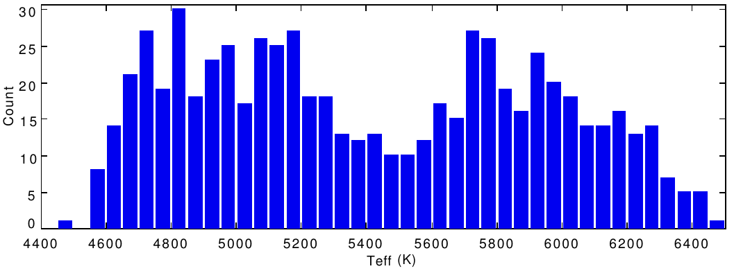
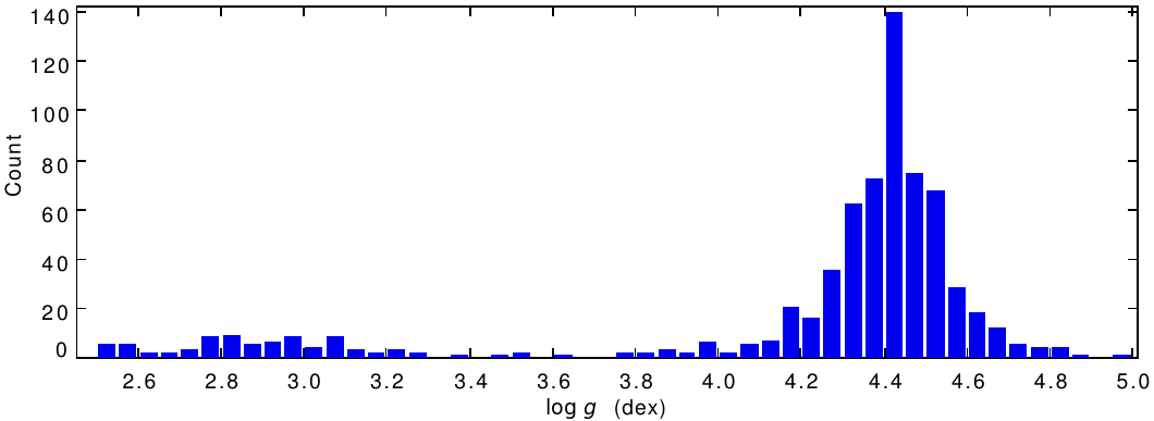
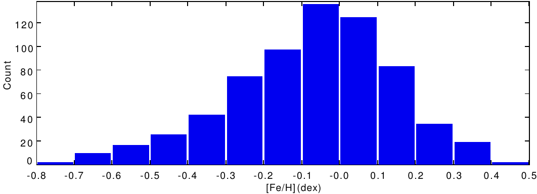
Figure 1: Histograms showing the parameter distribution of the validation sample. From top to bottom we show the $T_{\rm eff}$ , $\log g$, and [Fe/H] determined with spectroscopic methods.

3 Calibration

The main objective of this work is to build new $T_{\rm eff}$ and [Fe/H] spectroscopic calibrations for both FGK dwarfs and GK giants. This new calibration will be an improvement over the calibration presented in Sousa et al. (2012), hereafter the So12 calibration.

Here we present the $T_{\rm eff}$ calibration, the procedure of the [Fe/H] calibration and, finally, we describe an automatic code for producing these calibrations.

3.1 $T_{\rm eff}$ calibration

To perform the $T_{\rm eff}$ calibration, we used the relations between EW line-ratios, closely following Sousa et al. (2010). The basis of this technique is that metal lines have different sensitivities to $T_{\rm eff}$ and can be used in a similar way as in spectral type determinations. EW line-ratios are more precise than the use of EWs of individual lines (Gray, 1996, 2005; Kovtyukh et al., 2003; Sousa et al., 2010).

To fully exploit the advantages of EW line-ratios, some considerations were taken into account:

• The difference in excitation potential of the lines should be greater than 3 eV, ensuring that the lines have a different sensitivity to $T_{\rm eff}$ changes.

• The lines used for the ratios should not be too distant in wavelength ($\Delta\lambda<70\AA$) to minimize errors in continuum determination.

After compiling ratios that fulfilled the conditions described above for each star in the sample, we proceeded to refine the chosen ratios using additional selection criteria. We discarded ratios between lines that differed by more than two orders of magnitude in EW, thus removing ratios affected by poor measurements that are due to either poor Gaussian fitting or poor continuum fitting.

We also implemented a new selection cut-off based on the interquartile range method, IQR. This is a reliable method of statistical analysis that uses the statistical dispersion to effectively trim outliers (Upton et al., 1996). This has not been implemented in the previous works. The IQR measures the distance between the first and third quartiles of a distribution, $Q1$ and $Q3,$ respectively, and only considers values in the interval

$$[Q1-1.5\times IQR,Q3+1.5\times IQR].$$ (1)

The IQR method was used to remove the outliers in the distribution of each EW line-ratio, R_EW.

After the initial outlier-removal procedures, two functions were fitted to distributions of $T_{\rm eff}$ as a function of EW line-ratios: a linear function and a third-degree polynomial function. An additional outlier-removal procedure was then used based on a typical 2-$\sigma$ cut. Subsequently, we refitted the functions and obtained their coefficients. Figure 2 shows the 2-$\sigma$ cut procedure for the ratio between line Si i (6142.49 Å) and Ti i (6126.22 Å). This particular ratio was chosen as a consistency check to show how well our procedure compares with the one presented in Fig. 2 of Sousa et al. (2010).

Figure 2: Application of the 2-$\sigma$ cut to the ratio between the EW of line Si i (6142.49 Å) and of the EW of Ti i (6126.22 Å). The green line represents the third-degree polynomial fit, the dashed blue line represents the 2-$\sigma$ interval, and the black dots are the stars removed by the procedure. The vertical axis represents the spectroscopic $T_{\rm eff}$ and the horizontal axis represents the value of the EW ratios. The value of the final $\sigma$ of the fit, P_$\sigma$, is $\sim 82\ K$. The $\log g$ of each star is colour-coded.

Following Sousa et al. (2010), we then applied these methods to the inverse of the EW line-ratios, $1/R\_EW$, and to the logarithm of the EW line-ratios, $\log R\_EW$. The values of the standard deviation of every fitted function mentioned above were compared to select the function with the lowest standard deviation. This fitting procedure is shown in Fig. 3. The chosen function was the third-polynomial fit of the ratio R_EW, with a $\sigma\sim 86\ K$.

An additional validity check was implemented by accepting only functions that fitted two-thirds of the calibration sample. This ensured that each EW line-ratio used was valid for a significant number of the stars used in the calibration.

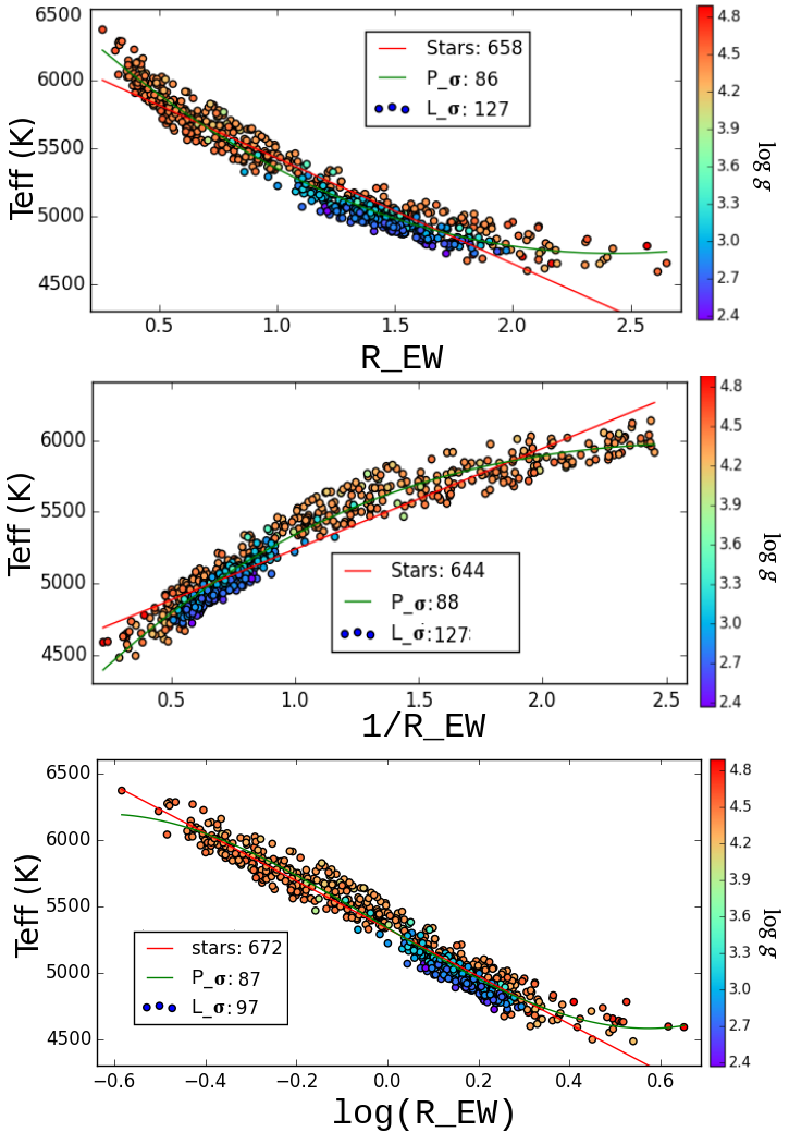
Figure 3: Fitting procedure for the $T_{\rm eff}$ calibration using the ratio, R_EW, between the EW of lines V i (5670.85 Å) and Fe i (5635.83 Å). We also show the fit for the inverse of the ratio, $1/R\_EW$, and the logarithm of the ratio, $\log R\_EW$. The final number of stars used in the fit, the standard deviation of the linear fit, L_$\sigma$, and of the third-degree polynomial fit, P_$\sigma$. The $\log g$ of each star is colour-coded.

3.2 Metallicity calibration

We calibrated the metallicity using only iron absorption lines, since we used the iron abundance as a proxy for stellar metallicity (Sousa et al., 2012). We discarded any ionized iron lines from the list because of their expected dependence on $\log g$.

The dependence on microturbulence was minimized by considering only weak lines (EW $<$ 70 $m\AA$). We also excluded lines with EW smaller than 20 $m\AA$, which minimized errors in the EW measurements that are due to the increased difficulty in estimating the continuum.

For each line, the calibration was obtained from the following equation:

$$\begin{split}EW=&C_{0}+C_{1}\times[Fe/H]+C_{2}\times\mbox{$T_{\rm eff}$ }+C_{3}\times[Fe/H]^{2}+\\ &C_{4}\times\mbox{$T_{\rm eff}$ }^{2}+C_{5}\times[Fe/H]\times\mbox{$T_{\rm eff}$ }\end{split}.$$ (2)

This equation represents the simple dependence of line strength on effective temperature and iron abundance and was solved for [Fe/H] by inverting the equation (Sousa et al., 2012). It is trivial to conclude that there will be a $T_{\rm eff}$ dependency for the [Fe/H] obtained from the inverted form of this equation.

We computed the [Fe/H] from Eq. 2 for each line and compared it with the spectroscopic values. The outliers were removed by first applying the IQR method, and a 2-$\sigma$ cut was then applied. The outliers obtained with this method are usually due to poorly measured EWs, caused by strong blending effects or poor continuum determination.

Two additional selection criteria were applied:

1. The slope of the comparison between the calibrated and spectroscopic [Fe/H] has to be within 3% of the identity line.

2. Only standard deviations of individual line calibrations lower than 0.06 dex were considered.

These conditions were empirically determined to achieve a balance between the largest number of lines possible and the highest precision possible. This balance ensures that we obtained statistical reliability while at the same time maintaining a high precision and accuracy in our calibration.

3.3 GeTCal

A useful by-product of our work in obtaining new calibrations was the creation of a Python code: GeTCal. GeTCal is a pratical implementation of the methods described in Sects. 3.1 and 3.2 and is capable of automatically producing $T_{\rm eff}$ and [Fe/H] calibrations. It requires three input parameters: a line list, the stellar parameters (and errors) of a sample of stars, and the measured EWs for each star. The calibrations can be used to compute the $T_{\rm eff}$ and [Fe/H] of stars of similar spectral classes. It is capable of performing the $T_{\rm eff}$ calibration, the [Fe/H] calibration, or both simultaneously.

The GeTCal code is built in such a way as to produce calibration files that are compatible with the TMCalc code (Sousa et al., 2012). This code is freely distributed and available for use by the community .

4 Results

In this section, we present the new calibration and test its application with TMCalc. We show consistency checks by comparing results obtained with the new calibration with those obtained with the So12 calibration for the joint sample. We present and analyze the results obtained when applying the new calibration to four independent stellar samples. Finally, we present and discuss the effect that an erroneous $T_{\rm eff}$ can have on [Fe/H] determination.

4.1 New calibration

Since our main goal is to obtain a new and more precise calibration with an increased range of applicability, accommodating both FGK dwarfs and GK-giant stars, we used the joint sample for calibration procedures.

Table 2 shows a summary of both calibrations. A total of 322 EW line-ratios and 101 Fe i are used in the new calibration, which is fewer than in the So12 calibration. The reason is that we consider stars in different evolutionary stages and, therefore, there are lines and ratios that are poor $T_{\rm eff}$ and [Fe/H] tracers for giants and dwarfs.

We calculated the $T_{\rm eff}$ using the So12 calibration for the joint sample. The top panel of Fig. 4 compares the computed $T_{\rm eff}$ with the spectroscopic $T_{\rm eff}$ . This calibration clearly does not fit either dwarfs in the low-temperature regime or giant stars properly, with a standard error of $112\ K$ and a mean difference of $-90\ K$ in $T_{\rm eff}$ . This behaviour was expected: the So12 calibration was created using only the So08 dwarfs, without the correction for the low-temperature regime (Tsantaki et al., 2013).

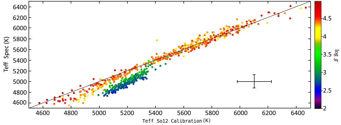
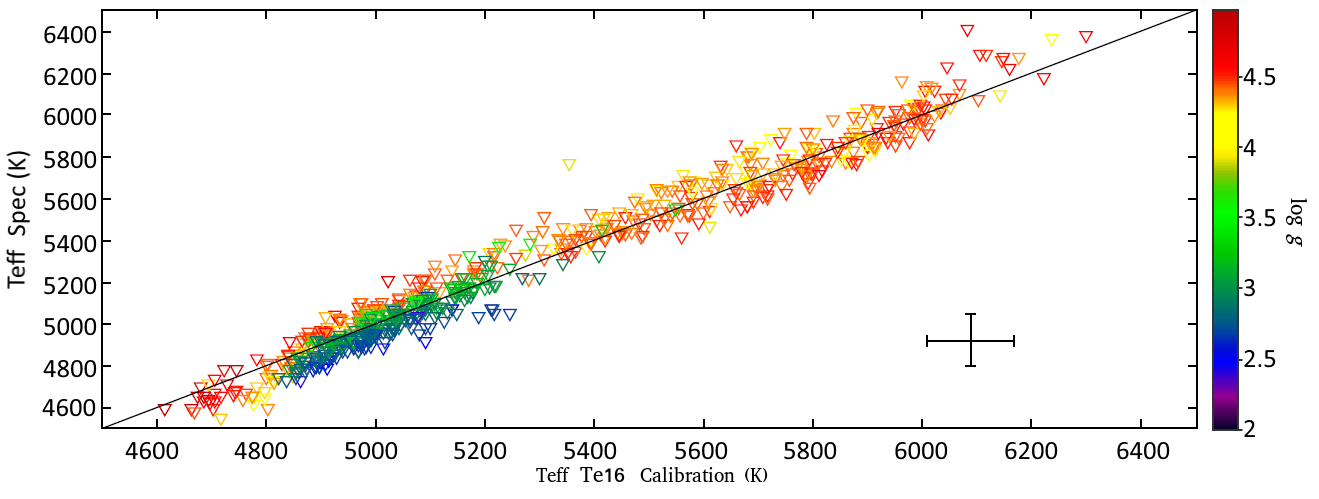
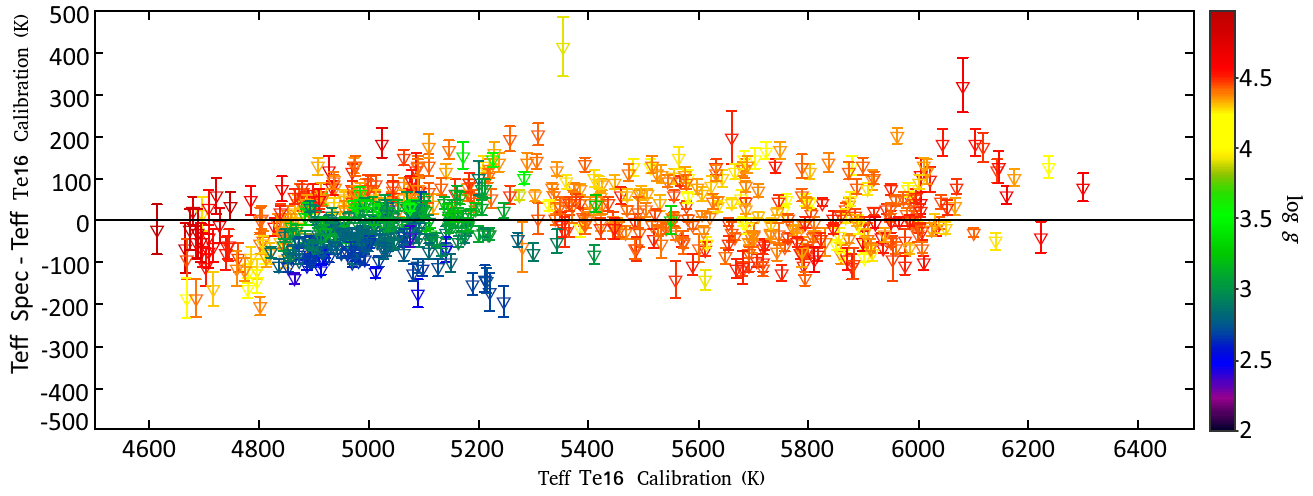
Figure 4: Comparison between the $T_{\rm eff}$ computed in this work and the spectroscopic values with the So12 calibration (top panel) and the Te16 calibration (middle panel) for the joint sample.  The line in the two plots represents the identity line, the standard deviation is plotted as the cross in both panels.  In the bottom panel we show the difference between the Te16 calibration and the spectroscopic $T_{\rm eff}$ as a function of $T_{\rm eff}$ , the error bars represent the errors in our computation.  The plots are colour-coded for $\log g$.

The middle panel of Fig. 4 shows the comparison of the temperature determination using the newly computed calibration (hereafter the Te16 calibration). There is a clear improvement compared to the So12 calibration, now with a standard deviation of $74\ K$ and a mean difference of the computed values of $-1\ K$.

The results for the metallicity computation of the joint sample are shown in Fig. 5. The So12 calibration forms a completely distinct locus for the GK-giant stars (top panel). On the other hand, the Te16 calibration removes the different locus for the GK giants of the sample (middle panel). We also plot the difference between the spectroscopic and computed [Fe/H] as a function of [Fe/H] (bottom panel). Most stars are well within $0.2$ dex from the zero value.

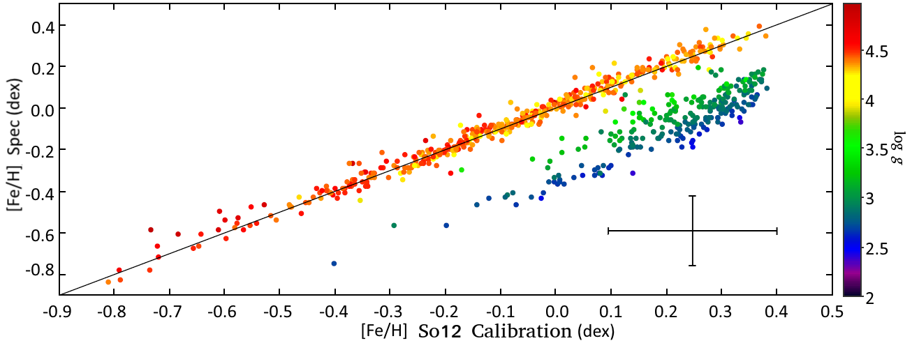
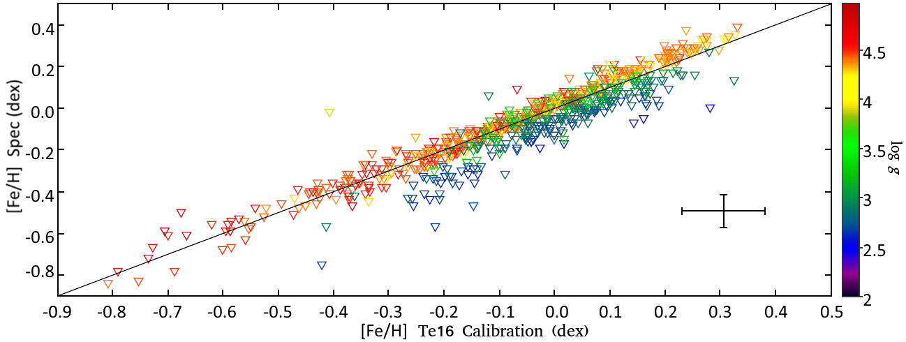
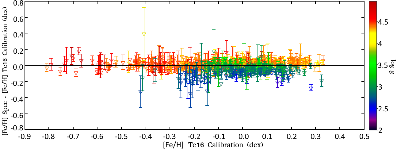
Figure 5: Comparison between the [Fe/H] computed in this work and the spectroscopic values for the So12 calibration (top panel) and the Te16 calibration (middle panel) for the joint sample.  The black line represents the identity line, the standard deviation is shown as the cross. The bottom panel shows the difference between [Fe/H] from spectroscopy and the one in this work as a function of [Fe/H], the error bars are the errors resulting from this work. The plots are colour-coded for $\log g$.

Table 3 shows the comparison between the two calibrations for the So08, Al15, and the joint samples. The mean difference between the spectroscopic and computed $T_{\rm eff}$ improves from $-90$ to $-1\ K$ when we apply the So12 calibration and the Te16 calibration for the joint sample, respectively. Likewise, there is an improvement in the mean difference in the values of [Fe/H], which is $-0.10\ dex$ for the So12 calibration and $-0.02\ dex$ for the Te16 calibration. The value of the computed $T_{\rm eff}$ standard deviations changes from $112\ K$ in the So12 calibration to $74\ K$ in the Te16 calibration, and the standard deviation of [Fe/H] improves from $0.15\ dex$ in the So12 calibration to $0.07\ dex$ of the Te16 calibration.

Table 2: Summary of the So12 and Te16 calibrations.

Calibration ratios Fe i_lines $T_{\rm eff}$ $\log g$ [Fe/H] (K) ($dex$) ($dex$) So12 $433$ $151$ [$4483,6403$] [$3.63,4.92$] [$-0.84,0.39$] Te16 $322$ $100$ [$4483,6403$] [$2.37,4.92$] [$-0.84,0.39$]

Table 3: Comparison of the So12 and Te16 calibrations and the spectroscopic values for the calibration samples.

Calibration Sample $\Delta$$T_{\rm eff}$ $\Delta$$T_{\rm eff}$ _median $\Delta$$T_{\rm eff}$ _$\sigma$ $\Delta$[Fe/H] $\Delta$[Fe/H]_median $\Delta$[Fe/H]_$\sigma$ (K) (K) (K) ($dex$) ($dex$) ($dex$) So12 So08 $-22$ $-21$ $69$ $0.00$ $0.00$ $0.04$ So12 Al15 $-208$ $-219$ $69$ $-0.29$ $-0.29$ $0.07$ So12 Joint $-90$ $-61$ $112$ $-0.10$ $-0.02$ $0.15$ Te16 So08 $17$ $23$ $76$ $0.01$ $0.02$ $0.04$ Te16 Al15 $-32$ $-36$ $58$ $-0.07$ $-0.06$ $0.08$ Te16 Joint $-1$ $-8$ $74$ $-0.02$ $0.00$ $0.07$

Table 4: Limits of applicability of the Te16 calibration.

$T_{\rm eff}$	$\log g$	[Fe/H]
(K)	($dex$)	($dex$)
$[4500,6500]$	$[2.5,4.9]$	$[-0.8,0.5]$

Table 5: Application of the Te16 calibration to the validation samples for stars within the applicability limits.

Sample $\Delta$$T_{\rm eff}$ $\Delta$$T_{\rm eff}$ _median $\Delta$$T_{\rm eff}$ _$\sigma$ $\Delta$[Fe/H] $\Delta$[Fe/H]_median $\Delta$[Fe/H]_$\sigma$ (K) (K) (K) ($dex$) ($dex$) ($dex$) GES $20$ $38$ $141$ $0.05$ $0.06$ $0.11$ Sa09 $-44$ $-41$ $75$ $-0.04$ $-0.06$ $0.10$ Gaia $43$ $40$ $91$ $0.08$ $0.09$ $0.18$ So11 $47$ $46$ $89$ $0.02$ $0.02$ $0.05$ Combined-validation $40$ $37$ $93$ $0.02$ $0.02$ $0.07$

A final remark should be made concerning the dependence of our values on $\log g$. Figures 4 and 5 are also colour-coded with $\log g$. A trend for low-$\log g$ stars in the Te16 calibration (middle panel) to have underestimated $T_{\rm eff}$ and [Fe/H] (e.g. giants with $\log g<2.5\ dex$) is evident. Although this trend has been greatly minimized, it is still present and should be taken into account when we consider the results of the new calibration. A partial justification for these discrepancies may be the fact that cooler stars in general have higher uncertainties in the EW determination. It should also be pointed out that this underestimation is within the standard deviation of the calibration. The limits of the Te16 calibration reflect the parameters of the calibration sample and are presented in Table 4.

4.2 Validation with independent samples

After obtaining the Te16 calibration for $T_{\rm eff}$ and [Fe/H], we applied it to four completely independent samples: the Sa09, Gaia, GES, and So11 samples.

Figure 6 shows the results of $T_{\rm eff}$ computed in this work against the $T_{\rm eff}$ determined by spectroscopy for the four validation samples and is colour-coded to the $\log g$ value. Stars outside the limits of the Te16 calibration ($\log g<2.5$) are not plotted in this figure.

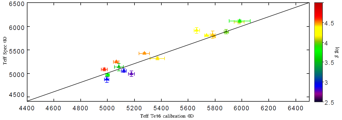
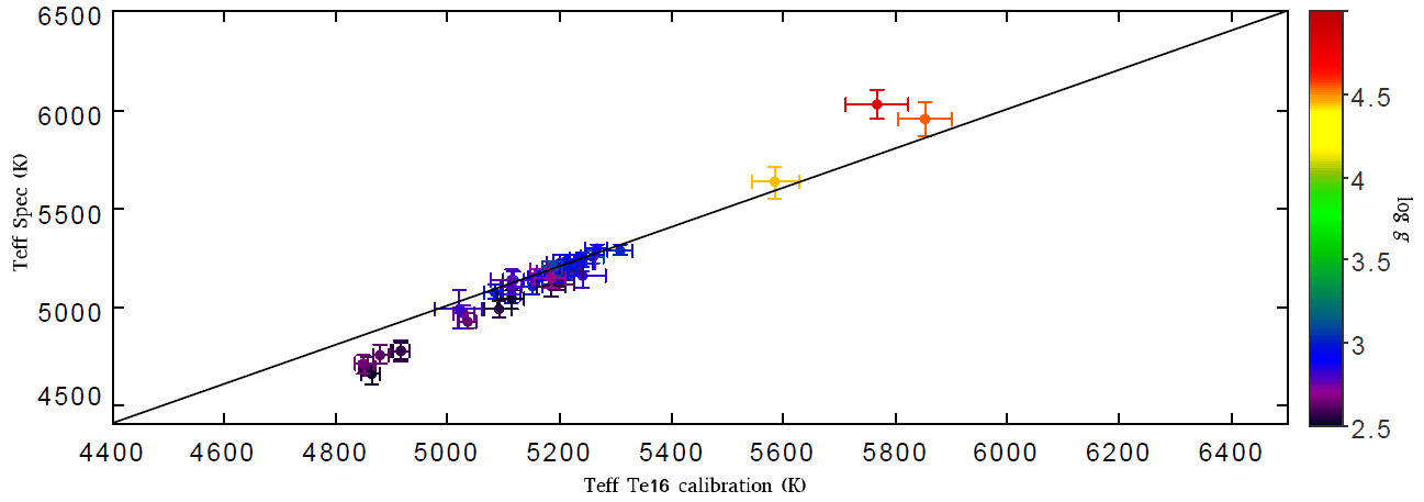
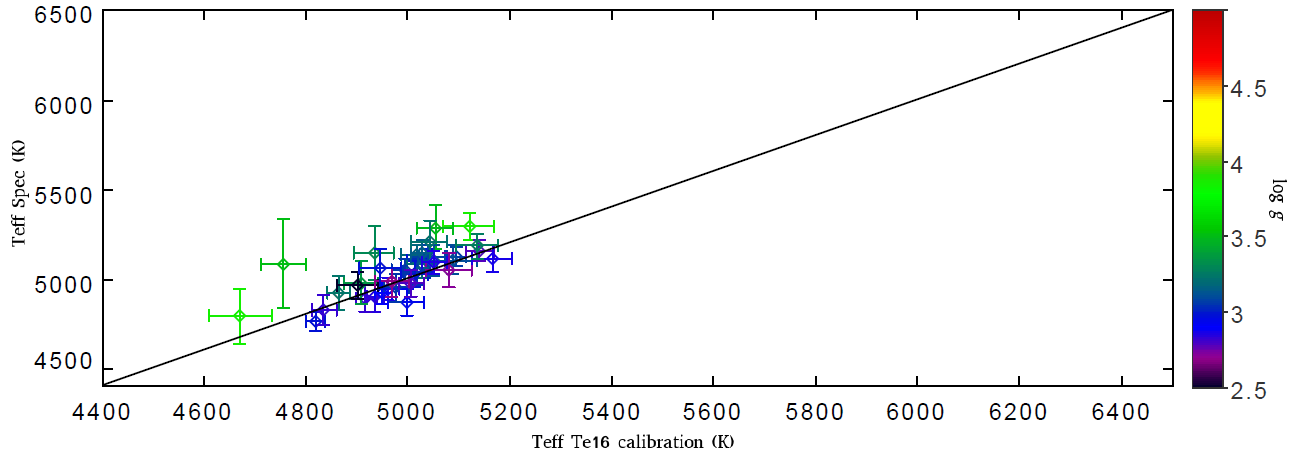
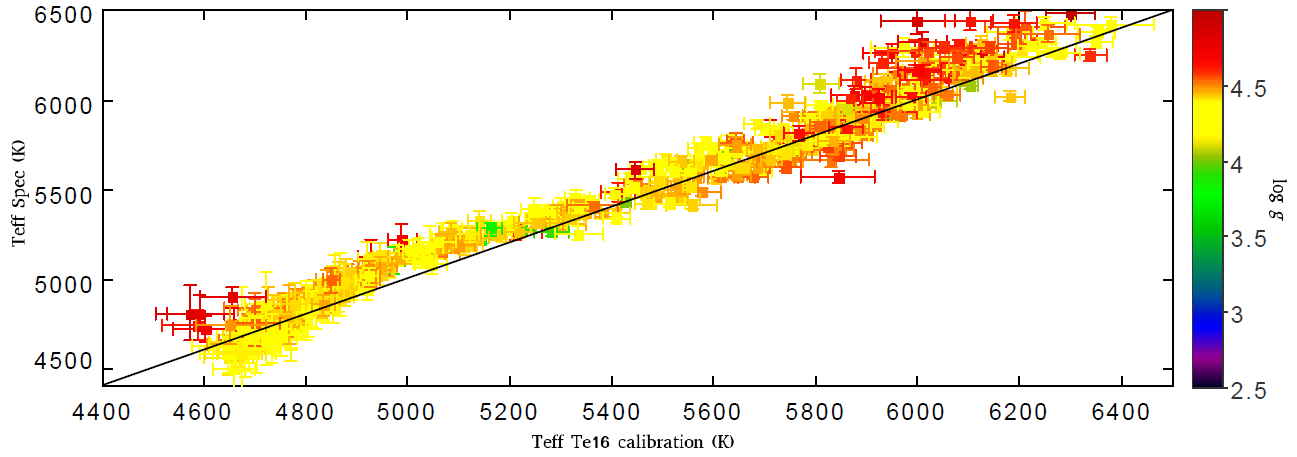
Figure 6: Comparison between the $T_{\rm eff}$ computed with TMCalc and the spectroscopic values with the Te16 calibration for the Gaia, Sa09, GES, and So11 sample from top to bottom. The colour-code represents the $\log g$ values and the black line represents the identity line. Only stars within the limits of applicability are plotted.

The results for the [Fe/H] computation of the independent samples are shown in Fig. 7, the same goodness-of-fit is evident in this plot for both samples. Again we encounter some outliers, but it should be made clear that these are stars with low-$\log g$ values and $T_{\rm eff}$ and, therefore, close to our applicability limits (see Table 4).

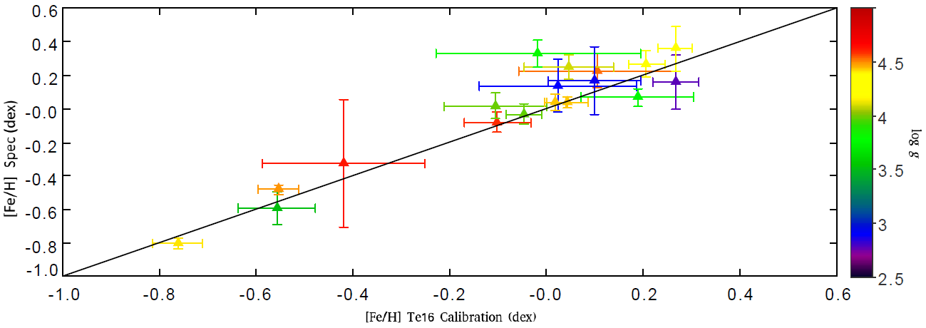
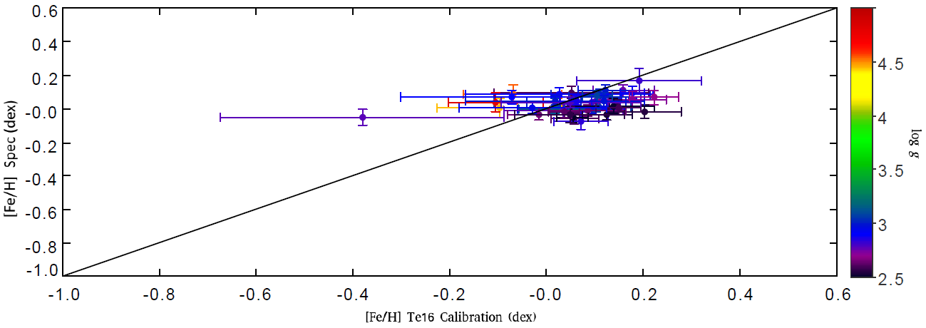
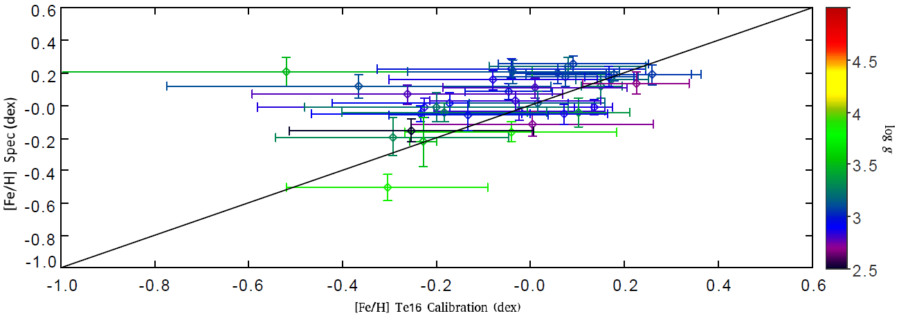
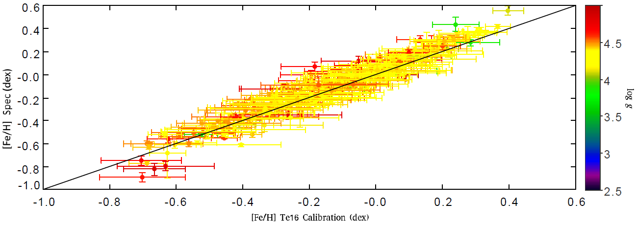
Figure 7: Comparison between the [Fe/H] computed with TMCalc and the spectroscopic values with the Te16 calibration for Gaia, Sa09, GES, and So11 sample. The colour-code represents the $\log g$ values and the black line represents the identity line. Only stars within the limits of applicability are plotted.

A summary of the application of the Te16 calibration to the various validation samples is provided in Table 5.

Applying the Te16 calibration to stars outside the applicability limits will introduce higher uncertainties. These applicability limits raise the question of how one should proceed when there is no prior knowledge of the $\log g$ of a star. Figure 8 shows the errors computed by TMCalc for $T_{\rm eff}$ and [Fe/H] as a function of $\log g$ for the Gaia, Sa09, and joint samples before the selection based on the applicability limits. Based on an empirical analysis of these plots, we propose that stars that simultaneously have [Fe/H] errors greater than $0.1\ dex$ and $T_{\rm eff}$ errors greater than $18\ K$ should be flagged for further examination because they may be outside, or close to, our applicability limits. The high errors can also be mimicked by low (S/N) spectra, therefore, this criterion is only an indication that the flagged stars need to be more carefully analysed. We tested this criterion and found that we would flag the stars with $\log g<2.5$ and obtain 62 stars ($\sim 10\%$), 4 stars ($\sim 19\%$), and 12 stars ($\sim 22\%$) as false positives, that is, stars that were flagged as suspicious but are not outside our applicability limits for the joint, Gaia, and Sa09 samples, respectively.

The errors obtained by TMCalc are computed considering the dispersion of the values given by all the individual calibrations, as independent of all others and, therefore, they are divided by the square root of the number of individual calibrations used. The error in [Fe/H] is obtained by using the 1-$\sigma$ temperature error. The final error is obtained from the quadratic sum of the two error sources (Sousa et al., 2012).

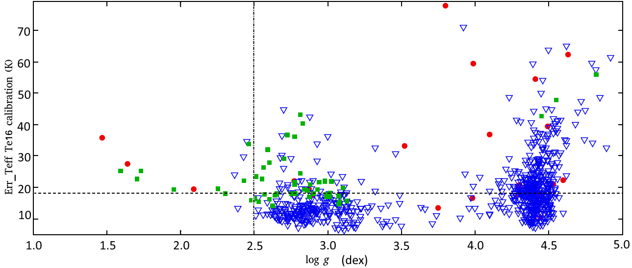
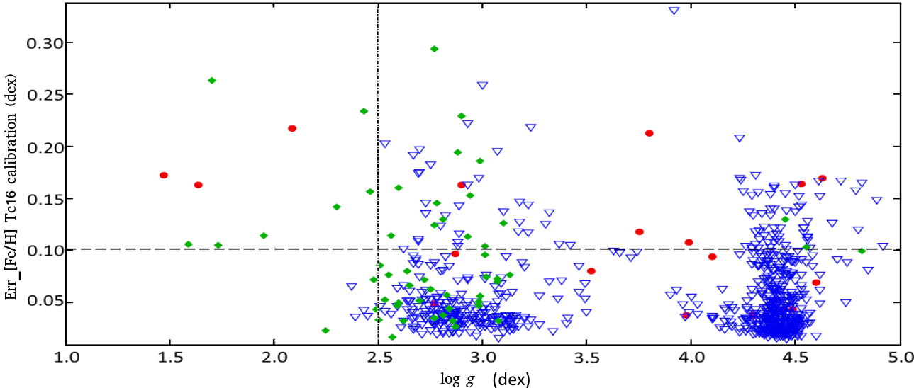
Figure 8: Errors in $T_{\rm eff}$ (top panel) and [Fe/H] (bottom panel) as a function of $\log g$. We plot the Gaia sample (red circles), the Sa09 sample (green diamonds), and the joint-sample (blue open triangles). The dashed lines represent the maximum error a measurement can have to be considered trustworthy, 18 K and 0.10 dex for $T_{\rm eff}$ and [Fe/H]. The vertical dot-dashed lines represent the $\log g$ limit of the Te16 calibration.

4.3 Effect of $T_{\rm eff}$ errors on [Fe/H]

As we discussed in Sect. 3.2, the [Fe/H] calibration has a non-negligible dependence on $T_{\rm eff}$ . TMCalc first computes the $T_{\rm eff}$ of a given star and then applies that value in the determination of [Fe/H]. To understand the effect of a poorly determined $T_{\rm eff}$ on the computations of [Fe/H], we performed the following test on the joint sample: we computed the [Fe/H] using the ARES+MOOG $T_{\rm eff}$ instead of the $T_{\rm eff}$ obtained from the application of the Te16 calibration.

Figure 9 shows the result of this computation. The [Fe/H] differences are below the 2-$\sigma$ of the new calibration and are therefore not significantly affected by the $T_{\rm eff}$ determination.

Additionally, Fig. 9 is also colour-coded to show the spectroscopic temperatures. With the exception of a few cooler stars, the dependence between $T_{\rm eff}$ and [Fe/H] computed appears to have a linear behaviour. When we consider that the [Fe/H] is computed by inverting Eq. 2, the apparent linearity is not a surprise because the inverted equation has a first-order dependence on $T_{\rm eff}$ .

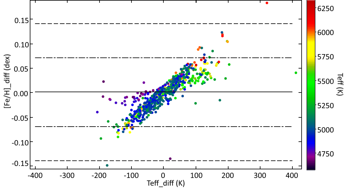
Figure 9: Effect of the spectroscopic $T_{\rm eff}$ on the [Fe/H] determination. The horizontal axis shows the difference between the spectroscopic value of $T_{\rm eff}$ and the one computed by TMCalc. The vertical axis shows the difference between the original computation of [Fe/H] and the value computed with the spectroscopic $T_{\rm eff}$ . The black line represents the zero of the vertical axis, the semi-dashed and the dashed black lines represent the 1-$\sigma$ and 2-$\sigma$ of the Te16 calibration, respectively.

5 Summary and conclusions

We presented new calibrations to obtain $T_{\rm eff}$ and [Fe/H] from the EWs of stellar spectra. These new calibrations are the first to successfully accommodate both FGK dwarfs and GK giants simultaneously, covering an increased range of spectral types and evolutionary stages. Our careful selection of the calibration sample and our improvement of the calibration method itself produced the calibrations presented in this work.

Using a joint sample of 451 FGK dwarfs and 257 GK giants, we determined new calibrations. These were applied and successfully tested against the pre-existing calibrations using the same sample. The Te16 calibration was applied to four different validation samples and was found to be effective within the range of $4500K<\mbox{$T_{\rm eff}$ }<6500K$, $2.5<\log g<4.9$ dex, and $-0.8<[Fe/H]<0.5$ dex, which covers most of FGK dwarfs and GK giants.

We showed that the dependence of the value of [Fe/H] on $T_{\rm eff}$ is within the error bars and therefore cannot be used to explain the poor estimates of [Fe/H] in the validation sample. This probably is the reason why these stars are outside our application range. We proposed a method to flag stars outside our applicability limits based on errors.

Future work should be focused on increasing the range of values of the calibration sample and, therefore, increasing the applicability limits of the calibration. Additional corrections are required to account for low-$\log g$ stars.

We built a Python code, GeTCal, that is capable of obtaining $T_{\rm eff}$ and [Fe/H] calibrations for any given sample of calibration stars. This program produces calibration files compatible with the existing TMCalc code and will therefore be distributed with future versions of TMCalc.

This work provides a fast way to determine stellar atmospheric parameters from spectrographic observations of FGK-dwarf and GK-giant stars. This calibration can be used to select targets for observations with future spectrographs such as ESPRESSO (Pepe et al., 2014).  It can also be expanded to other spectral types by applying the GeTCal code and an appropriate calibration sample.