Controlling Feynman diagrammatic expansions: physical nature of the pseudo gap in the two-dimensional Hubbard model

Abstract

We introduce a method for summing Feynman’s perturbation series based on diagrammatic Monte Carlo that significantly improves its convergence properties. This allows us to investigate in a controllable manner the pseudogap regime of the Hubbard model and to study the nodal/antinodal dichotomy at low doping and intermediate coupling. Marked differences from the weak coupling scenario are manifest, such as a higher degree of incoherence at the antinodes than at the ‘hot spots’. Our results show that the pseudogap and reduction of quasiparticle coherence at the antinode is due to antiferromagnetic spin correlations centered around the commensurate $(\pi,\pi)$ wavevector. In contrast, the dominant source of scattering at the node is associated with incommensurate momentum transfer. Umklapp scattering is found to play a key role in the nodal/antinodal dichotomy.

Introduction and context.

Strongly-correlated many-electron systems are a major theoretical challenge. Numerical approaches face difficulties brought by the exponentially large Hilbert space or the fermionic sign problem. Among the many questions still open, an outstanding one is the nature of the low doping and intermediate to strong coupling regime of the prototypical two-dimensional Hubbard model. Unbiased methods are needed to establish whether key aspects of cuprate phenomenology, such as the opening of a pseudogap and the associated nodal/antinodal (N/AN) dichotomy Timusk and Statt (1999); Badoux et al. (2016), are intrinsic features of the model, and to settle the much debated physical origin of these phenomena. Recently, cluster-DMFT approaches have allowed significant progress on these issues Georges et al. (1996); Maier et al. (2005); Sénéchal and Tremblay (2004); LeBlanc et al. (2015). However, cluster methods lack fine momentum resolution Gull et al. (2010), which is crucial in view of the strong momentum dependence along the Fermi surface, and in establishing which fluctuations are responsible for the physics Gunnarsson et al. (2015), e.g. distinguishing commensurate and incommensurate fluctuations.

A promising alternative method is the diagrammatic Monte Carlo (DiagMC) technique Prokof’ev and Svistunov (1998); Van Houcke et al. (2008); Kozik et al. (2010), based on the stochastic summation of Feynman diagrammatic series directly in the thermodynamic limit, which in principle enables controlled solutions with arbitrary momentum resolution. However, for lattice systems, fundamental problems with series convergence have so far limited its scope of application to modest couplings, relatively high temperature and/or low density. In particular, the skeleton series built on the full (interacting) Green’s function $G$ can converge to a wrong answer Kozik et al. (2015), whereas the bare series built on the non-interacting Green’s function $G_{0}$ does not exhibit misleading convergence but typically diverges in the strongly-correlated regime.

In this Letter, we introduce an approach that considerably enlarges the applicability range of DiagMC. It is based on a parametric modification of the bare diagrammatic series that improves its convergence properties. This technique allows us to address the pseudogap regime of the 2D Hubbard model at small doping and intermediate coupling. The high momentum resolution and direct access to scattering processes in DiagMC allows us to identify the physical origin of the pseudogap and N/AN dichotomy, which are shown to result from antiferromagnetic spin correlations. At the node, the transfer momentum $\mathbf{q}$ of relevant modes is found to be incommensurate, connecting Fermi surface points. In contrast, at the antinode, scattering with commensurate momentum exchange $\mathbf{q}=(\pi,\pi)$ dominates. We find that quasiparticles are more incoherent at the antinode than at the ‘hot spots’ ( where the Fermi surface intersects the antiferromagnetic zone boundary), thus establishing the strong-coupling nature of the regime investigated. We show that the umklapp scattering enhanced at large perturbation orders plays a key role in this suppression of coherence.

The method: action optimization and recursive evaluation of diagrams.

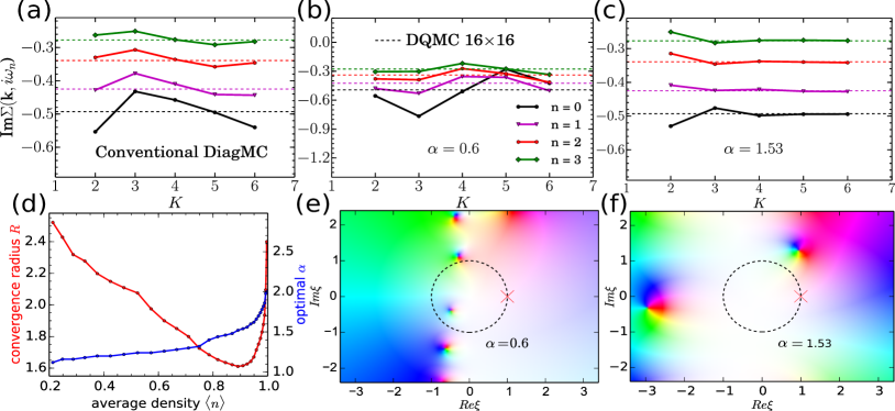
Figure 1: Top row: Imaginary part of the Hubbard model self-energy at the first four Matsubara frequencies obtained as a sum of the first $K$ perturbation orders. The parameters are $U=4.0$, $t^{\prime}=-0.3$, $\mu=0$, $n\sim 0.725$, $T=0.5$. The dashed lines are a benchmark from determinantal QMC simulations on a $16\times 16$ lattice (the discrete time interval is $\Delta\tau=0.0375$ where the Trotter error is negligible). (a): Standard series with Hartree diagrams included in bare Green’s function, (b): $\alpha$-shifted case with $\alpha=0.6$, (c): the optimal case $\alpha=1.53$. Bottom row: Results for the atomic limit $t=0$, $U=4$, $T=0.5$, $\mu=0.138$, $n\sim 0.725$. (e) and (f): Modulus/phase (displayed as saturation/hue) map of the self-energy in the complex $\xi$-plane for $\alpha=0.6$ and $\alpha=1.53$ respectively. The physical solution is at the cross $\xi=1$ on the unit circle. (d): Optimal $\alpha$ and corresponding maximal convergence radius as a function of the density $\langle n\rangle$ in the Hubbard atom.

We study the Hubbard model on an (infinite) square lattice:

$$\mathcal{H}=-\sum_{ij\sigma}t_{ij}\,c^{\dagger}_{i\sigma}c_{j\sigma}+U\sum_{i}n_{i\uparrow}n_{i\downarrow},$$ (1)

with hopping amplitudes $t$ and $t^{\prime}$ between nearest-neighbour and next nearest-neighbour sites respectively, and use $t=1$ as our energy unit. In essence, DiagMC is an efficient way of computing the coefficients $a_{l}$ of a perturbative series for the self-energy as a function of the Matsubara frequency $\omega_{n}$ and momentum $\mathbf{k}$:

$$\Sigma(i\omega_{n},\mathbf{k})=\lim_{L\to\infty}\sum_{n=1}^{L}a_{l}(i\omega_{n},\mathbf{k})U^{l},$$ (2)

where $a_{l}$ is a sum of all one particle irreducible (1PI) Feynman diagrams with $l$ interaction vertices connected by non-interacting Green’s functions $G_{0}(i\omega_{n},\mathbf{k})=[i\omega_{n}-\epsilon_{\mathbf{k}}+\mu]^{-1}$ Abrikosov et al. (1975). The success of this approach fundamentally relies on the convergence properties of the series (2). Because $a_{l}$ are stochastically computed in DiagMC as the sums of factorial (in $l$) number of sign-alternating contributions, in practice one can only reach $L=6\sim 7$ with reasonable statistical error bars due to the fermionic sign problem. Thus, a controlled answer is only warranted as long as the series (2) can be reliably extrapolated to $L\to\infty$ given an essentially limited number of computed expansion orders. This extrapolation becomes increasingly difficult at low $T$ and large $U$.

In order to establish control over the convergence properties of the series, we introduce a modified action $S_{\xi}$ given by

$$S_{\xi}=-\sum_{\omega_{n},\mathbf{k},\sigma}c_{\omega_{n},\mathbf{k},\sigma}^{\dagger}\tilde{G_{0}}(i\omega_{n},\mathbf{k})^{-1}c_{\omega_{n},\mathbf{k},\sigma}$$ (3)

$$-\xi\sum_{\omega_{n},\mathbf{k},\sigma}\alpha_{\mathbf{k}}(i\omega_{n})c_{\omega_{n},\mathbf{k},\sigma}^{\dagger}c_{\omega_{n},\mathbf{k},\sigma}+\xi U\int_{0}^{\beta}n_{\tau\uparrow}n_{\tau\downarrow}d\tau,$$

where $\tilde{G}_{0}(i\omega_{n},\mathbf{k})^{-1}=i\omega_{n}+\mu-\epsilon_{\mathbf{k}}-\alpha_{\mathbf{k}}(i\omega_{n})=G_{0}(i\omega_{n},\mathbf{k})^{-1}-\alpha_{\mathbf{k}}(i\omega_{n})$ and $\alpha_{\mathbf{k}}(i\omega_{n})$ is an arbitrary auxiliary field (cf. Rubtsov et al. (2005); Profumo et al. (2015); Rossi et al. (2016)); at $\xi=1$ we recover the original action for the Hamiltonian (1). Expanding in powers of $\xi$ and applying Wick’s theorem generates a new diagrammatic representation of $\Sigma$:

$$\Sigma(i\omega_{n},\mathbf{k})=\lim_{M\to\infty}\sum_{m=1}^{M}\tilde{a}_{m}(i\omega_{n},\mathbf{k})\xi^{m},$$ (4)

Here the coefficient $\tilde{a}_{m}$ is a sum of all the diagrams for $a_{l}$ with $l$ running from $1$ to $m$, and for each diagram of order $l$, an additional sum over all possible ways of inserting $m-l$ instances of $\alpha_{\mathbf{k}}(i\omega_{n})$ in the fermionic lines is performed according to the standard diagrammatic rules of expanding with respect to an external field Abrikosov et al. (1975). Note that here the bare propagators $G_{0}(i\omega_{n},\mathbf{k})$ are now replaced with $\tilde{G_{0}}(i\omega_{n},\mathbf{k})$. The freedom in choosing $\alpha_{\mathbf{k}}(i\omega_{n})$ can be now used to control the convergence properties of the modified series (4) at $\xi=1$.

This freedom comes at the expense of extending the diagrammatic space, which considerably worsens the sign problem. To make practical calculations feasible we introduce a recursive protocol for summing all the diagrams for $\tilde{a}_{m}$, which makes use of the already computed $\tilde{a}_{n}$, $n<m$. The idea is that a high-order diagram may contain (between propagator lines) self-energy insertions of lower orders; all possible insertions of the total order $p$ can be implicitly summed and integrated over the internal momentum/frequency variables by including the results for $\tilde{a}_{n}$, $n\leq p$ in the propagator lines:

$$G^{(p)}=\sum_{n=0}^{p}G^{(n)}\tilde{a}_{p-n}\xi^{p-n}\tilde{G}_{0},\;\;\;p>0,\;\;\;G^{(0)}\equiv\tilde{G}_{0},$$ (5)

so that $G^{(p)}\propto\xi^{p}$. Then $\tilde{a}_{m}$ can be obtained by DiagMC sampling of only 1PI skeleton diagrams of order $l=\{1,\ldots,m\}$, where in each diagram some bare propagators $\tilde{G_{0}}$ are randomly replaced by dressed propagators $G^{(p_{i})}$ so that $\sum_{i}p_{i}=m-l$. This recursive approach substantially improves the efficiency of DiagMC by effectively reducing the configuration space and can be generalized to other channels, e.g. by introducing dressed interaction lines $W^{(p)}$, dressed two-particle irreducible vertices $\Gamma^{(p)}$, etc.

Illustrative result at high $T/t$.

We first investigate the simplest case of a constant field $\alpha_{\mathbf{k}}(i\omega_{n})\equiv\alpha$. In Fig. 1, we illustrate its effect on the Hubbard model at $U=4$ and $T=0.5$, using determinantal QMC simulation on a $16\times 16$ lattice as a benchmark Blankenbecler et al. (1981). In the first row of Fig. 1, we compare the value of $\Sigma(\mathbf{k},i\omega_{n})$ at the first few Matsubara frequencies and $\mathbf{k}=(\pi/4,\pi)$ summed up to order $K$, i.e. $\Sigma(\mathbf{k},i\omega_{n})=\sum_{m=1}^{K}\tilde{a}_{m}(\mathbf{k},n)\xi^{m}$. Fig. 1a shows the behaviour of the standard series (2) (with the Hartree diagrams included in the Green’s function following Refs. Van Houcke et al. (2008); Kozik et al. (2010)), Fig. 1b and Fig. 1c show the behavior for two different choices of $\alpha$. Clearly, the standard series and the one for an arbitrarily selected $\alpha=0.6$ fail to converge within accessible orders. However, a clever choice of $\alpha=1.53$ yields a great improvement of convergence. The exact result is recovered already at order $4$ and the extrapolation of the series to infinite order is straightforward.

Rationale: pole-moving.

In order to get insight into the improvement brought by the introduction of a modified action, we study in details the limiting case $t=0$, the Hubbard atom, which can be solved exactly. In particular, we show how tuning $\alpha$ allows to control the convergence radius of the series (4). The self-energy for the action $S_{\xi}$ and $t=0$ is given by

$$\Sigma(i\omega_{n}) =\frac{n\xi U}{2}+\frac{1}{4}\frac{n(2-n)\xi^{2}U^{2}}{i\omega_{n}+\tilde{\mu}-(2-n)\xi U/2}$$ (6)

$$\tilde{\mu} =\xi\alpha-\alpha+\mu$$ (7)

where $n=[e^{\beta\tilde{\mu}}+e^{2\beta\tilde{\mu}-\beta\xi U}]/[1+2e^{\beta\tilde{\mu}}+e^{2\beta\tilde{\mu}-\beta\xi U}]$ is the density. The analytical structure of $\Sigma(i\omega_{0})$ in the complex-$\xi$ plane is shown in Fig. 1e and Fig. 1f. The convergence radius $R$ of the series expansion in $\xi$ is given by the distance from the origin to the closest pole in the complex-$\xi$ plane, which strongly depends on the value of $\alpha$. For $\alpha=0.6$ a pole is closer to the origin than the evaluation point $\xi=1$ and the series diverges, whereas for $\alpha=1.53$ the poles are further away and the series is convergent at $\xi=1$. When $\alpha$ is further increased, new poles get closer to the origin and there is therefore an optimal value for $\alpha$ for which the radius of convergence is maximal. A systematic study for the full Hubbard model at $T=0.5$ suggests an optimal value of $\alpha\simeq 1.53$, close to this atomic estimate $\alpha\sim 1.3$ , as expected from a similar analytic structure of $\Sigma$ at this high temperature. Thus the Hubbard atom can provide a reasonable guide for finding the optimal $\alpha$. Finally, we find the largest convergence radius and the corresponding optimal $\alpha$ for different densities of the Hubbard atom, as displayed in Fig. 1d. We see that $R$ is infinite at half-filling and becomes finite ($R\lesssim 2.5$) as soon as a doping is introduced. For $U=4$, the convergence radius is always large enough for the series to converge. It has a minimum $R\simeq 1.6>1$ around $10\%$ hole (or electron) doping.

Reaching the pseudogap scale.

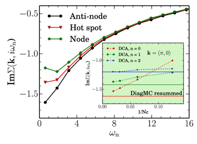
Figure 2: Imaginary part of the self-energy at the node, hot-spot and anti-node at $U=5.6$, $t^{\prime}=-0.3$, $n=0.96$, $T=0.2$. Inset: DCA results with cluster size $N_{c}=8$, $16$, $32$, $52$ extrapolate to the DiagMC-summed result at different frequencies.

We now show that this improved scheme allows one to reach the pseudogap region Tremblay et al. (2006); Sordi et al. (2012); Macridin et al. (2006); Gull et al. (2013). We consider the Hubbard model at $4\%$ hole doping and $U=5.6$, $t^{\prime}=-0.3$. We could achieve convergence down to $T=0.2$, where we compute the self-energy up to 7^th order with an optimized $\alpha=2.3$. In Fig. 2, we display the imaginary part of the self-energy $\mathrm{Im}\Sigma(\mathbf{k},i\omega_{n})$ taken at three different momenta $\mathbf{k}$ on the Fermi surface (FS). We see that the self-energy behaves differently at the nodal point $\mathbf{k}_{N}=(1.47,1.47)$ (intersection of the FS with the zone diagonal) in comparison to the antinode $\mathbf{k}_{AN}=(3.04,0.49)$ (where the FS hits the upper zone boundary). The imaginary part of the AN self-energy extrapolates to a larger negative value at low-frequency, indicating strongest correlation effects at the AN. Hence, a clear N/AN differentiation is already apparent at $T=0.2$, consistently with previous calculations Macridin et al. (2005); Tremblay et al. (2006) indicating that this temperature coincides with the onset of the pseudogap at $U=5.6$. The inset of Fig. 2 also demonstrates that our results at the AN are in excellent agreement with large scale dynamical cluster approximation (DCA)(Maier et al., 2005) ones (after extrapolating the latter as a function of cluster size). Finally, we note (Fig. 2) that the self-energy is larger at the AN than at the ‘hot-spot’ $\mathbf{k}_{HS}=(2.26,0.88)$ (intersection of the FS with the antiferromagnetic zone boundary), indicating that we have reached a regime in which the weak-coupling spin-fluctuation picture does not apply. Being able to resolve the difference of behaviour at the HS and AN is a clear advantage of the current approach as compared to cluster methods.

Physical origin of the nodal/antinodal dichotomy: antiferromagnetic spin correlations.

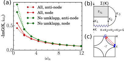
Figure 3: (a): Imaginary part of the Green’s functions at node and anti-node as a function of frequency, in cases with and without umklapp processes. (b): Decomposition of the self-energy using the Dyson-Schwinger equation of motion, c.f. Eq. 8. (c): Illustration of a typical weak-coupling umklapp process with $G=(2\pi,2\pi)$.

A decisive asset of DiagMC is that it provides direct information about the mechanisms behind the pseudogap and N/AN differentiation. We demonstrate that umklapp processes are essential to the destruction of the AN quasiparticles. To this aim, we decompose the self-energy as shown in Fig. 3b and monitor the momentum entering the two-particle scattering amplitute $F_{\uparrow\downarrow}$ during the DiagMC evaluation. By forcing the sum of incoming and outcoming momenta of $F_{\uparrow\downarrow}$ to differ by a non-zero or zero reciprocal lattice vector $G$, we allow or forbid umklapp scattering at will. The results are given in Fig. 3: when umklapp processes are forbidden, both the imaginary part of N and AN Green’s functions become significantly larger, indicating that umklapp processes are relevant to suppress spectral weight in the full solution. More importantly, without umklapp processes AN Green’s function turns out to be more coherent than the N one, while the opposite is true when umklapp processes are allowed. They are therefore a key ingredient in the suppression of spectral weight at the AN, and their importance is actually found to grow as the perturbation order increases (not shown).

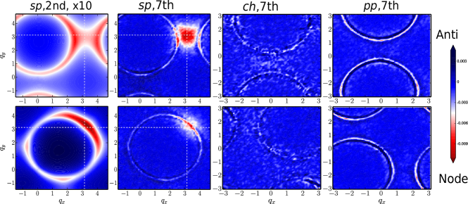
Figure 4: Maps of the transfer momentum $\mathbf{q}$ contributions to $\mathrm{Im}\Sigma(\mathbf{k},i\omega_{0})$ + $\mathrm{Im}\Sigma(\mathbf{k},i\omega_{1})$ in the spin (sp), charge (ch) and particle-particle (pp) channels, both at the node, $\mathbf{k}=(1.47,1.47)$ (bottom row) and anti-node, $\mathbf{k}=(3.04,0.49)$ (top row). The two panels on the left are results at perturbation order 2 while the rest are obtained up to order 7.

To analyse further the N/AN dichotomy, we employ the Dyson-Schwinger equation representing the self-energy at a given momentum $\mathbf{k}$ as (Fig. 3b):

$$\Sigma(\mathbf{k})=\frac{Un}{2}-\sum_{\mathbf{k^{\prime}},\mathbf{q}}F_{\uparrow\downarrow}(\mathbf{k},\mathbf{k^{\prime}},\mathbf{q})g(\mathbf{k})g(\mathbf{k^{\prime}}+\mathbf{q})g(\mathbf{k}+\mathbf{q}),$$ (8)

or $\Sigma(\mathbf{k})=\frac{Un}{2}-\sum_{\mathbf{q}}[\Sigma^{\mathbf{q}}_{X}(\mathbf{k})]$, and study the contributions from different collective modes with the transfer momentum $\mathbf{q}$, where $X$ stands for spin (sp), charge (ch) or particle-particle (pp) representations,

$$\Sigma_{sp}^{\mathbf{q}}(\mathbf{k}) = \sum_{\mathbf{k^{\prime}}}-F_{\uparrow\downarrow}(\mathbf{k},\mathbf{k}+\mathbf{q},\mathbf{k^{\prime}}-\mathbf{k})g(\mathbf{k^{\prime}})g(\mathbf{k^{\prime}}+\mathbf{q})g(\mathbf{k}+\mathbf{q})$$

$$\Sigma_{ch}^{q}(\mathbf{k}) = \sum_{\mathbf{k^{\prime}}}[F_{\uparrow\downarrow}(\mathbf{k},\mathbf{k}+\mathbf{q},\mathbf{k^{\prime}}-\mathbf{k})$$

$$-2\times F_{\uparrow\downarrow}(\mathbf{k},\mathbf{k^{\prime}},\mathbf{q})]g(\mathbf{k^{\prime}})g(\mathbf{k^{\prime}}+\mathbf{q})g(\mathbf{k}+\mathbf{q})$$

$$\Sigma_{pp}^{\mathbf{q}}(\mathbf{k}) = \sum_{\mathbf{k^{\prime}}}-F_{\uparrow\downarrow}(\mathbf{k},\mathbf{k^{\prime}},\mathbf{q}-\mathbf{k}-\mathbf{k^{\prime}})g(\mathbf{k^{\prime}})g(\mathbf{q}-\mathbf{k^{\prime}})g(\mathbf{q}-\mathbf{k})$$

The above equations are obtained by expressing $F_{sp/ch/pp}$ in terms of $F_{\uparrow\downarrow}$ (see Gunnarsson et al. (2015)). The resulting low-energy intensity maps of $\Sigma^{\mathbf{q}}_{X}(\mathbf{k})$ (obtained at order 7) for all three representations at the N and at the AN are displayed in Fig. 4. The first compelling result is that the charge and the particle-particle representations are essentially featureless for both the N and AN self-energies. The only visible patterns stem from FS to FS transfer momenta, as shown by the light circles. In contrast, the spin channel exhibits dominant modes responsible for the largest contribution to the imaginary part of the self-energy at low-energies. Interestingly, the most significant transfer momenta are all close to $(\pi,\pi)$ and we conclude that antiferromagnetic spin correlations are the leading scattering mechanism in the pseudogap region of the phase diagram, in agreement with recent experimental findings Badoux et al. (2016). The fine momentum resolution of DiagMC allows us to examine the difference between the N and AN self-energy in further detail. We see that, at the N the transfer momenta are close, but not exactly at $(\pi,\pi)$. They are concentrated around the Fermi surface and are not exactly commensurate. On the contrary, at the AN the transfer momenta are centered around $(\pi,\pi)$ and the corresponding amplitude is larger. The existence of a saddle-point in the band dispersion (van-Hove singularity) close to the AN may be at the origin of this difference, the flatter dispersion allowing to compensate for the energetic cost of commensurate $(\pi,\pi)$ spin scattering. The relevance of the saddle-point has been discussed in Refs.Hur and Rice (2009); Furukawa et al. (1998); Honerkamp et al. (2001) within weak-coupling approaches. Importantly, we note (Fig. 4) that FS scattering involving an incommensurate transfer momentum controls the nodal self-energy at both low and high perturbation orders. In contrast, $(\pi,\pi)$ scattering emerges at high perturbation orders at the AN. Hence, the scattering mechanism remains of the weak-coupling type at the N, while the pseudogap opening at the AN is a strong-coupling phenomenon for the value of $U/t$ studied here.

Conclusions and perspectives.

In this letter, we have introduced an improved DiagMC method relying on an optimized parametric modification of the Hubbard model action. This allows us to access in a controlled way and with high momentum resolution parameter regimes that were previously unreachable, such as the onset of the pseudogap and nodal/antinodal differentiation. We show that these effects are due to antiferromagnetic correlations and that marked differences with weak-coupling spin-fluctuation theories appear in the regime of coupling investigated here. The challenge ahead is to improve the current method in order to reach significantly lower temperatures.