Alpha-decay energies of superheavy nuclei for the Fayans functional

Abstract

Alpha-decay energies for several chains of super-heavy nuclei are calculated within the self-consistent mean-field approach by using the Fayans functional FaNDF⁰. They are compared to the experimental data and predictions of two Skyrme functionals, SLy4 and SkM*, and of the macro-micro method as well. The corresponding lifetimes are calculated with the use of the semi-phenomenological formulas by Parkhomenko and Sobiczewski and by Royer and Zhang.

I Introduction

During the last decade, remarkable progress has been achieved in a synthesis of superheavy nuclei belonging to the so-called “stability island”, the elements with charge numbers $Z\simeq 114-120$, predicted about fifty years ago Myers-Swiat ; Strut . Two isotopes of the element with $Z=116$, named later Lv, and one with $Z=118$ were created first by Oganessian et. al. Oganes_2006 . After the element $118$ two isotopes of the element $Z=117$ were synthesized Oganes_2010 . The latter element was investigated in more details in Refs. Oganes_2011 ; Oganes_2012 ; Oganes_2013 ; Z117_new . An attempt Oganes_2009 to create the element with $Z=120$ turned out to be unsuccessful, however, evidently, efforts in this direction will be continued.

In fact, the stability island turned out to be “the stability shallow”, as all of these new nuclei are not stable. Although their lifetimes are large in the “nuclear scale”, they are usually not sufficiently long lived to be detected in a usual way. All of them undergo alpha-decay, and the authors of the experimental works cited above detected, for each primary nucleus, a chain of several alpha-decays by measuring the alpha-decay energies $E_{\alpha}$ with high accuracy, and the respective lifetimes $T_{\alpha}$, leading to a nucleus which was already known. Therefore, a theoretical support is desirable to make such kind of indirect identification of the new superheavy nuclei more reliable.

For even-even nuclei, in which the transition occurs between the $0^{+}$ ground states, the alpha-decay energies $E_{\alpha}(Z,N)$ are determined, with allowance for the recoil effect, in terms of the mass difference between nuclei related by alpha decay:

$$Q_{\alpha}(Z,N)=M(^{A}_{Z}X_{N})-M(^{A-4}_{Z-2}Y_{N-2})-M_{\alpha}.$$ (1)

For odd and odd-odd nuclei, a correction to this simple formula could appear due to a possible excitation of the parent and/or daughter nucleus which may occur in the real experimental situation.

In Refs. Oganes_2006 ; Oganes_2010 ; Oganes_2011 ; Oganes_2012 ; Oganes_2013 , the experimental data for $Q_{\alpha}$ were compared with predictions Muntian-1 ; Muntian-2 of the so-called macro-micro method (MMM) MMM ; MMM_1 . In this method, the binding energy of a nucleus is found as the sum of two terms, a macroscopic energy which was calculated on the basis of the liquid-drop model and a shell correction energy which was found according to the Strutinsky method Strut . Thus, two independent sets of parameters are used in the MMM, one for the nuclear droplet model and the second for the Shell Model potential. In general, such a comparison confirmed the identification of new superheavy nuclei. Recently, in a comprehensive study of superheavy nuclei Heenen-2015 , predictions of the MMM, including $\alpha$-decay characteristics, were compared to those from the nuclear energy density functional (EDF) method. Two Skyrme EDFs were used, SkM* skms and SLy4 sly4to7 , for which the parametrizations can be also found in the review article criteria . A relativistic EDF DD-PC1 DD-PC1 was also used for a comparison. The main bulk of calculations was carried out within the self-consistent mean-field (SCMF) approach. In addition, several examples of beyond mean-field results were presented which explicitly considered collective correlations related to the symmetry restoration and fluctuations of the collective coordinates. It was shown that the SCMF described well $\alpha$-decay and $\beta$-decay energies. At the same time, beyond mean-field corrections are important in order to find the correct deformation energy curves and fission barrier heights.

The finite-range EDF by Fayans et al. Fay1 ; Fay4 ; Fay was used first to find $Q_{\alpha}$ for new superheavy $\alpha$-chains in Ref. alpha-13 , within a partially self-consistent calculation, with an approximate consideration of the deformation energy. The total binding energy of a deformed nucleus was presented as a sum of two terms, $E_{B}(N,Z)=E_{\rm sph}(N,Z)+E_{\rm def}(N,Z)$, where the main, spherical one, was found for a Fayans EDF, whereas the “deformation” addendum was taken from published tables for two Skyrme EDFs. To be definite, a version DF3-a DF3-a of the initial Fayans EDF DF3 Fay4 ; Fay was used for the spherical energy. For the deformation energy, the EDF HFB-17 HFB-17 ; site was used for nuclei with $Z\leq 110$ and MSk7 MSk7 , for $Z>110$. Accuracy of such semi-self-consistent calculations turned out to be only a bit worse compared to that of the MMM approach.

The absence of a deformed Fayans EDF solver was the reason of the use of such non-consistent ansatz in Ref. alpha-13 . Recently, however, such a code has been developed Fay-def . A localized version FaNDF⁰ Fay5 of the general finite range Fayans EDF was used, making the surface term more similar to the Skyrme one. This allowed to employ, with some modifications, the computer code HFBTHO code , developed originally for Skyrme EDFs. First applications of this code to deformed nuclei Fay-def ; Fay-def1 ; drip-2n ; Pb-def with the use of the original set of parameters of the EDF FaNDF⁰ Fay5 found for spherical nuclei turned out to be rather successful. The goal of the present work is to provide a new, completely self-consistent, calculation of $Q_{\alpha}$ energies for six superheavy $\alpha$-chains with the Fayans EDF. For a comparison, calculations with two Skyrme EDFs, SLy4 and SkM*, are carried out. These two parametrizations are rather commonly employed in various Skyrme EDF calculations. In particular, they were used as representatives of non-relativistic EDFs in Heenen-2015 . Thus, this part of our calculations repeats that of Heenen-2015 and partly earlier study of (Cwi99) . With these two Skyrme parametrizations, when considering low-lying collective excitations in spherical nuclei, the older SkM* was found more successful than SLy4 BE2-SHF . Predictions of the self-consistent methods are compared to the MMM of Refs. Muntian-1 ; Muntian-2 .

Theoretical predictions for $Q_{\alpha}$ are important not only by itself but also to find the lifetime $T_{\alpha}$. Indeed, the latter is governed mainly by the exponential Gamow factor Gamow , which is found almost unambiguously in terms of $Q_{\alpha}$ by finding the penetrability of the Coulomb barrier in the daughter nucleus for an emitted alpha particle. Unfortunately, at the present there is no a reliable microscopic theory for the pre-exponential factor as this is a very complicated many-body problem. It is worth mentioning recent studies in this direction Peltonen ; Betan ; micr1 ; Ward . Some of them are rather promising but do not provide a simple tool for systematic calculations. In such a situation, the phenomenological approaches are more practical. Most of them are close to the classical Viola-Seaborg formula VS , which involves seven phenomenological parameters. Here, just as in alpha-13 , we use the five-parameter modification of this formula Par-Sobich by Parkhomenko and Sobiczewski (PS). For a comparison, similar calculations were repeated with the use of more recent 12-parameter formula by Royer and Zhang (RZ) Royer .

II Fayans EDF predictions for $Q_{\alpha}$ values in superheavy nuclei

In this section, we give the SCMF predictions of the Fayans EDF FaNDF⁰ Fay5 for six $\alpha$-decay chains which begin from the following parent superheavy nuclei: ${}^{294}118$, ${}^{294}117$, ${}^{293}117$, ²⁹¹Lv, ${}^{288}115$, and ${}^{287}115$. For completeness, we write down explicitly the main ingredients of this EDF. In the Fayans method, the ground state energy of a nucleus is considered as a functional of normal density $\rho$ and anomalous density $\nu$, as

$$E_{0}=\int{\cal E}[\rho({\bf r}),\nu({\bf r})]d^{3}r,$$ (2)

where the isotopic indices and the spin-orbit densities are omitted for brevity.

The volume part of the EDF, ${\cal E}^{\rm v}(\rho)$, is taken as a fractional function of densities $\rho_{+}=\rho_{n}+\rho_{p}$ and $\rho_{-}=\rho_{n}-\rho_{p}$:

$${\cal E}^{\rm v}(\rho)=C_{0}\left[a^{\rm v}_{+}\frac{\rho_{+}^{2}}{4}f^{\rm v}_{+}(x)+a^{\rm v}_{-}\frac{\rho_{-}^{2}}{4}f^{\rm v}_{-}(x)\right],$$ (3)

where

$$f^{\rm v}_{+}(x)=\frac{1-h^{\rm v}_{1+}x^{\sigma}}{1+h^{\rm v}_{2+}x^{\sigma}}$$ (4)

and

$$f^{\rm v}_{-}(x)=\frac{1-h^{\rm v}_{1-}x}{1+h^{\rm v}_{2-}x}.$$ (5)

Here, $x=\rho_{+}/\rho_{0}$ is the dimensionless nuclear density, $\rho_{0}=2(k_{\rm F}^{0})^{3}/3\pi^{2}$ being the equilibrium symmetric nuclear matter density. The coefficient $C_{0}=(dn/d\varepsilon_{\rm F})^{-1}=\pi^{2}/(k_{\rm F}^{0})m)$ is the usual normalization factor used in the theory of finite Fermi system (TFFS) AB1 , the inverse density of states at the Fermi surface. The power parameter $\sigma=1/3$ is chosen in the FaNDF⁰ functional, in contrast to the case for DF3 or DF3-a, where $\sigma=1$ is used. The dimensionless parameters in Eqs. 3–5 are the same as in Fay5 : $a^{\rm v}_{+}=-9.559$, $h^{\rm v}_{1+}=0.633$, $h^{\rm v}_{2+}=0.131$, $a^{\rm v}_{-}=4.428$, $h^{\rm v}_{1-}=0.25$, and $h^{\rm v}_{2-}=1.300$. They correspond to the following characteristics of nuclear matter: the equilibrium density $\rho_{0}=0.160$ fm^-3 (the corresponding mean radius parameter is $r_{0}=1.143$ fm), the energy per particle $\mu=-16.0$ MeV, the incompressibility $K_{0}=220$ MeV, and the asymmetry energy coefficient of $a_{\rm sym}=30.0$ MeV. Higher derivatives of the EDF of nuclear matter over the densities $\rho_{+},\rho_{-}$, suggested in criteria for the Skyrme EDFs as a set of criteria for functionals, are given in Fay-def for the FaNDF⁰ functional.

If one sets $h^{\rm v}_{2+}=h^{\rm v}_{2-}=0$, the volume part of the Fayans EDF reduces to the form typical for Skyrme EDFs. As was discussed in detail in Fay-def , the “Fayans denominator” and the use of the bare mass $m^{*}=m$, both peculiarities of the Fayans EDF method, are generically related to the self-consistent TFFS KhS , reflecting in a hidden form the energy-dependence effects inherent to this approach.

Until recently, the Fayans EDF was applied to spherical nuclei only. These applications were rather successful, in comparison with analogous Skyrme Hartree-Fock-Bogoliubov (HFB) calculations. They included the analysis of the magnetic mu1 ; mu2 and quadrupole QEPJ ; QEPJ-Web moments in odd nuclei, of characteristics of the first $2^{+}$ excitations in even semi-magic nuclei BE2 ; BE2-Web , of charge radii Sap-Tolk , and of beta-decay Borz as well. In addition, single-particle spectra of seven magic nuclei was described with high accuracy Levels . A short review comparison of predictions of Fayans and Skyrme EDFs for these phenomena in spherical nuclei was given in Ref. compar-spher , and more detailed one, in Ref. compar-YAF .

The use of the local approximation for the Yukawa finite-range function, ${\rm Yu}(r)\to 1-r_{c}^{2}\nabla^{2}$, in the DF3-like EDFs leads to the following structure of the surface term of the FaNDF⁰ functional:

$${\cal E}^{\rm s}(\rho)=C_{0}\frac{1}{4}\frac{a^{\rm s}_{+}r_{0}^{2}(\nabla\rho_{+})^{2}}{1+h^{\rm s}_{+}x^{\sigma}+h^{\rm s}_{\nabla}r_{0}^{2}(\nabla x_{+})^{2}},$$ (6)

with $h^{\rm s}_{+}=h^{\rm v}_{2+}$, $a^{\rm s}_{+}=0.600$, $h^{\rm s}_{\nabla}=0.440$. This approximation is the main point which permitted in Fay-def to modify the Skyrme HFB computer code HFBTHO code for the Fayans EDF. This code solves the HFB equations in axially symmetric harmonic oscillator basis by assuming time-reversal symmetry.

Here, just as in Fay-def , we use a two-parameter form for the anomalous term of the EDF:

$${\cal E}_{\rm anom}=C_{0}\sum_{i=n,p}\nu_{i}^{{\dagger}}({\bf r})f^{\xi}(x_{+}({\bf r}))\nu_{i}({\bf r}),$$ (7)

where the density-dependent dimensionless effective pairing force is

$$f^{\xi}(x_{+})=f^{\xi}_{\rm ex}+h^{\xi}x_{+}.$$ (8)

Two models for pairing will be used, the volume one with $h^{\xi}=0$, and the surface model, with $h^{\xi}\simeq-f^{\xi}_{\rm ex}$. As we use the zero-range pairing force, a cut-off should be used in solving the gap equation. Here we use the same cut-off energy $E_{\rm cut}=60$ MeV as in Fay-def . The standard procedure to solve the HFB equations is used. The code code for Skyrme EDFs and its analogue for the Fayans EDF used in Fay-def and here makes it possible to restore particle number approximately within the Lipkin–Nogami scheme. Its effect is significant for the total pairing energy but negligible (about $0.1$–$0.2\;$MeV) for the binding energy differences entering to the $Q_{\alpha}$ values.

For odd nuclei, we used the equal filling approximation for the quasiparticle blocking prescription when solving the HFB equations. We stress that, within this prescription, the mean-field of the odd (or odd-odd) nucleus is solved fully self-consistently. The equal filling approximation has been examined in many works, for example, in Refs. odd1 ; odd2 . In the latter, it was estimated that this approximation introduces inaccuracy of the order of $0.1$–$0.2\;$MeV for the binding energy. This is much smaller than the differences between various EDFs for the predicted $Q_{\alpha}$ values.

Pairing interaction influences significantly the one-neutron separation energies

$$S_{n}(N,Z)=B(N,Z)-B(N-1,Z).$$ (9)

In figure 1, they are shown for uranium isotopes, calculated with the FaNDF⁰ EDF, with two models of pairing specified above. The corresponding values of the parameters of Eq. (8) are ($f^{\xi}=-0.440,\,h^{\xi}=0$) for the volume pairing and ($f^{\xi}=-1.433,\,h^{\xi}=1.375$) for the surface one. In this work, the calculation scheme for the Fayans EDF is the same as that in Ref. Fay-def for the uranium chain. In particular, the HFB equations were solved in a basis of 25 oscillator shells. Comparison is made with experimental data mass and predictions from the Skyrme EDF HFB-17 EDF HFB-17 ; site . We see that the Fayans EDF with both pairing models reproduce experimental data sufficiently well, with an accuracy comparable with that of the Skyrme EDF HFB-17.

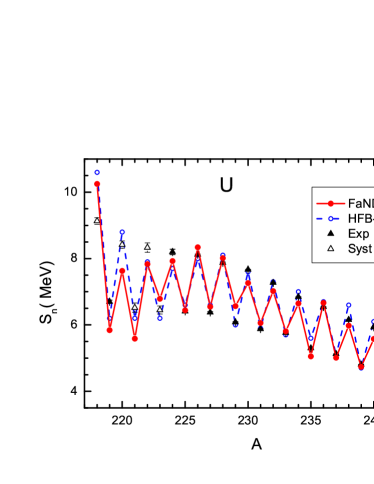
Figure 1: The $S_{n}$ values for the U isotopic chain.

Next, we investigate the alpha-decay energies $Q_{\alpha}$. The results of calculations are presented in figure 2 and in Table 1. For the Fayans EDF, predictions of the volume and surface pairing are given. A comparison is made with the data and predictions of two Skyrme EDFs, the SLy4 sly4to7 and SkM* skms . Corresponding results are found by us with the use of the code code . In this case, 20 oscillator shells were used, in accordance with msu . For both of the Skyrme EDFs, the mixed pairing is used code :

$$V_{\rm pair}^{n,p}({\bf r},{\bf r}^{\prime})=V_{0}^{n,p}\left(1-\alpha\frac{\rho({\bf r})}{\rho_{c}}\right)\delta({\bf r}-{\bf r}^{\prime}),$$ (10)

$\alpha=0.5$, with obvious notation. The paring strength is taken to be the same for neutrons and protons, namely $V_{0}^{n}=V_{0}^{p}=-259.0\;$MeV. For completeness, we included also predictions of the MMM method taken from the tables in Muntian-1 , $Z=102$–109, and Muntian-2 , $Z=110$–120. Several empty places in the MMM column of Table 1 are caused with absence of the corresponding values in the tables cited above.

A remark should be made about the experimental $Q_{\alpha}$ values used in the tables and figures 2–7. They are taken mainly from the references cited in the caption of Table 1, where the alpha-energies $E_{\alpha}$ were measured, and $Q_{\alpha}$ being found by accounting the recoil effect. This recipe may be doubtful in the case of odd and odd-odd nuclei where the $\alpha$-transition between ground states can be forbidden, and the observed transition may connect excited states. The analysis of the lifetimes $T_{\alpha}$ may help to clear up this point. They will be analyzed in the next Section. There are also cases when experimental $Q_{\alpha}$ values are not available. In this kind of situation we use estimated masses from mass systematics of Ref. mass . They are shown with the open triangles in the figures.

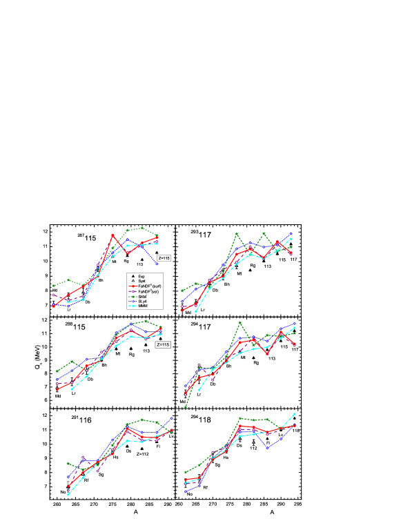
Figure 2: The $Q_{\alpha}$ values for alpha decay chains starting from nuclei ${}^{287}115$, ${}^{293}117$, ${}^{288}115$, ${}^{294}117$, ²⁹¹Lv, and ${}^{294}118$. Theoretical results are shown for FaNDF⁰ with surface and volume pairing, for SkM* and SLy4 Skyrme EDFs, and for the MMM model. These are compared to experimental and estimated values.

Table 1: $\alpha$-decay energies $Q_{\alpha}$ (MeV) of superheavy nuclei. In each line, $Z$ and $A$ correspond to the parent nucleus. FaNDF⁰(surf) and FaNDF⁰(vol) denote the Fayans EDF with the surface and volume pairing, correspondingly. Experimental data are taken from Oganes_2006 (^a)), Z117_new (^b)), Oganes_2013 (^c)), mass , compilation of several experiments, (^d)), Oganes_2005 (^e)). The estimated data (^(syst)) are taken from the systematics in mass .

Nuclei	FaNDF0(surf)	FaNDF0(vol)	SLy4	SkM*	MMM	Exp.
${}^{294}{\rm 118}$	11.278	11.310	11.364	11.330	12.11	11.81 (0.06)$\,{}^{a)}$
290Lv	11.116	10.981	10.354	11.074	11.08	10.99 (0.08)$\,{}^{a)}$
286Fl	10.847	10.683	9.719	11.734	10.86	10.37 (0.06)$\,{}^{a)}$
282Cn	11.188	11.005	10.886	11.688	10.68	10.11 (0.2)$\,{}^{(\rm syst)}$
278Ds	11.272	11.026	10.849	11.802	10.54	10.37 (0.2)$\,{}^{(\rm syst)}$
274Hs	9.497	9.788	9.870	9.932	9.55	9.57 (0.2)$\,{}^{(\rm syst)}$
270Sg	8.913	9.407	9.004	9.319	8.74	8.99 (0.3)$\,{}^{(\rm syst)}$
266Rf	7.617	7.316	7.052	8.508	7.05	7.55 (0.3)$\,{}^{(\rm syst)}$
262No	7.497	7.210	6.649	7.932	6.86	7.25 (0.3)$\,{}^{(\rm syst)}$
294117	10.225	10.131	11.629	11.033	11.43	11.20 (0.04)$\,{}^{b)}$
290115	11.117	10.898	10.143	10.792	10.65	10.45 (0.04)$\,{}^{b)}$
286113	9.494	9.479	8.792	10.879	9.98	9.79 (0.05)$\,{}^{c)}$
282Rg	10.524	10.701	10.037	11.512	9.85	9.18 (0.03)$\,{}^{b)}$
278Mt	10.334	9.681	9.851	10.442	9.55	9.59 (0.03)$\,{}^{b)}$
274Bh	8.957	9.187	8.911	9.285	8.83	8.97 (0.03)$\,{}^{b)}$
270Db	7.966	7.528	7.643	8.376	8.34	8.02 (0.03)$\,{}^{b)}$
266Lr	7.717	8.663	7.993	8.449	6.79	7.57 (0.3)$\,{}^{(\rm syst)}$
262Md	6.564	6.431	6.011	7.621	-	6.5 (0.3)$\,{}^{(\rm syst)}$
293117	10.605	10.502	10.976	10.990	11.53	11.18 (0.05)$\,{}^{d)}$
289115	11.356	11.167	10.035	10.688	10.74	10.52 (0.05)$\,{}^{d)}$
285113	10.271	10.154	9.592	11.900	10.21	10.03 (0.05)$\,{}^{d)}$
281Rg	10.850	11.003	10.719	11.736	10.48	9.41 (0.05)$\,{}^{c)}$
277Mt	10.498	9.956	10.007	10.618	9.84	9.71 (0.2)$\,{}^{(\rm syst)}$
273Bh	9.014	9.456	9.170	9.386	8.89	9.06 (0.3)$\,{}^{(\rm syst)}$
269Db	8.596	8.739	7.902	8.305	8.17	8.49 (0.3)$\,{}^{(\rm syst)}$
265Lr	7.162	7.021	7.208	8.503	6.62	7.23 (0.2)$\,{}^{(\rm syst)}$
261Md	6.708	6.960	6.400	8.030	-	6.75 (0.4)$\,{}^{(\rm syst)}$
291Lv	10.959	10.987	10.557	10.798	10.91	10.89 (0.07)$\,{}^{a)}$
287Fl	10.463	10.243	9.130	11.528	10.56	10.16 (0.06)$\,{}^{a)}$
283Cn	10.506	10.275	10.499	11.731	10.16	9.67 (0.06)$\,{}^{a)}$
279Ds	11.097	10.876	10.234	11.361	10.24	9.84 (0.06)$\,{}^{a)}$
275Hs	9.321	9.606	9.600	9.920	9.41	9.44 (0.06)$\,{}^{a)}$
271Sg	8.747	8.115	8.554	8.541	8.71	8.67 (0.08)$\,{}^{a)}$
267Rf	7.998	9.077	8.046	8.204	-	7.89 (0.3)$\,{}^{(\rm syst)}$
263No	7.031	6.759	6.287	8.634	6.45	7.0 (0.4)$\,{}^{(\rm syst)}$
288115	11.376	10.968	9.389	11.485	10.95	10.61 (0.06)$\,{}^{e)}$
284113	10.661	10.588	10.393	11.930	10.68	10.15 (0.06)$\,{}^{e)}$
280Rg	11.208	11.274	11.023	11.717	10.77	9.87 (0.06)$\,{}^{e)}$
276Mt	10.681	10.393	10.490	10.919	10.09	9.85 (0.06)$\,{}^{e)}$
272Bh	8.978	9.612	8.836	9.128	9.08	9.02 (0.06)$\,{}^{e)}$
268Db	8.598	8.245	8.514	8.239	7.90	8.26 (0.3)$\,{}^{e)}$
264Lr	7.343	7.334	6.606	8.902	6.84	7.4 (0.3)$\,{}^{(\rm syst)}$
260Md	6.823	7.259	6.919	8.189	-	6.94 (0.3)$\,{}^{(\rm syst)}$
287115	11.628	11.362	9.840	11.772	11.21	10.59 (0.09)$\,{}^{e)}$
283113	11.264	11.090	10.990	12.269	11.12	10.12 (0.09)$\,{}^{e)}$
279Rg	10.494	10.607	11.489	12.107	11.08	10.37 (0.16)$\,{}^{e)}$
275Mt	11.789	11.726	10.585	10.909	10.34	10.33 (0.09)$\,{}^{e)}$
271Hs	9.010	9.760	9.557	9.425	9.07	9.49 (0.16)$\,{}^{(\rm syst)}$
267Db	8.312	7.667	7.412	8.378	7.41	7.9 (0.3)$\,{}^{(\rm syst)}$
263Lr	7.742	7.355	6.979	8.744	7.26	7.68 (0.2)$\,{}^{(\rm syst)}$
259Md	6.968	7.737	7.091	8.352	-	7.11 (0.2)$\,{}^{(\rm syst)}$

By eye, the accuracy of the MMM is higher compared to self-consistent approaches. Among the latest EDFs, the Fayans one, with both the models for pairing, has the accuracy comparable with both the Skyrme ones. To estimate it quantitatively, we present in Table 2 the differences

$$\delta Q_{\alpha}=Q_{\alpha}^{\rm theor}-Q_{\alpha}^{\rm exp},$$ (11)

with obvious notation. In the last column, the mark “(syst)” is used for the mass systematics data given in Ref. mass . In the last line of the table, values are given of the root-mean-square deviation (RMSD) of the theory under consideration from the experiment:

$$\langle\delta Q_{\alpha}\rangle_{\rm rms}=\sqrt{\frac{1}{N}\sum_{i}\left(Q_{\alpha,i}^{\rm theor}-Q_{\alpha,i}^{\rm exp}\right)^{2}}.$$ (12)

From the $\delta Q_{\alpha}$ results, we can see that the MMM exceeds in accuracy all the self-consistent methods used, with its RMSD being smaller by a factor of 1.5–2. However, it is worth to note that the MMM parameters, those of the liquid-drop model and of the Saxon-Woods shell-model potential, were fitted in Ref. Muntian-1 ; Muntian-2 to characteristics of heavy deformed nuclei in the uranium region, close to the nuclear map region under consideration. Per contra, the main part of the EDFs parameters is universal for all nuclei. Among the self-consistent calculations presented, the SLy4 EDF results in the highest accuracy. The Fayans EDF has approximately 10 % worse RMSD. However, it is worth reminding that the FaNDF⁰ parameters were fitted in Fay5 to characteristics of the spherical nuclei only of the region between calcium and lead chains. Evidently, more fine tuning of this EDF parameters is necessary, including heavy deformed nuclei into the fitting procedure. Accuracy of the SkM* EDF is approximately two times worse comparing to other EDFs used.

Table 2: Differences in Eq. (11) between theoretical predictions of $\alpha$-decay energies of superheavy nuclei from Table 1 and the corresponding experimental data. The mark “(syst)” in the last column denotes the data from the systematics in mass .

Nuclei	FaNDF0(surf)	FaNDF0(vol)	SLy4	SkM*	MMM	data from
294118	-0.532	-0.500	-0.446	-0.480	0.300	Oganes_2006
290Lv	0.126	-0.009	-0.636	0.084	0.090	Oganes_2006
286Fl	0.477	0.313	-0.651	1.364	0.490	Oganes_2006
282Cn	1.078	0.895	0.776	1.578	0.570	mass (syst)
278Ds	0.902	0.655	0.479	1.432	0.170	mass (syst)
274Hs	-0.073	0.218	0.300	0.362	-0.020	mass (syst)
270Sg	-0.078	0.417	0.014	0.329	-0.250	mass (syst)
266Rf	0.067	-0.234	-0.498	0.958	-0.500	mass (syst)
262No	0.247	-0.040	-0.601	0.682	-0.390	mass (syst)
294117	-0.975	-1.069	0.429	-0.167	0.230	Z117_new
290115	0.667	0.448	-0.307	0.342	0.200	Z117_new
286113	-0.296	-0.311	-0.998	1.089	0.190	Oganes_2013
282Rg	1.344	1.521	0.857	2.332	0.670	Z117_new
278Mt	0.744	0.091	0.261	0.852	-0.040	Z117_new
274Bh	-0.013	0.217	-0.059	0.315	-0.140	Z117_new
270Db	-0.054	-0.492	-0.377	0.356	0.320	Z117_new
266Lr	0.147	1.093	0.423	0.879	-0.780	mass (syst)
262Md	0.064	-0.069	-0.489	1.121	-	mass (syst)
293117	-0.575	-0.678	-0.204	-0.190	0.350	mass
289115	0.836	0.647	-0.485	0.168	0.220	mass
285113	0.241	0.124	-0.438	1.870	0.180	mass
281Rg	1.440	1.593	1.309	2.326	1.070	Oganes_2013
277Mt	0.788	0.246	0.297	0.908	0.130	mass (syst)
273Bh	-0.046	0.396	0.110	0.326	-0.170	mass (syst)
269Db	0.106	0.249	-0.588	-0.185	-0.320	mass (syst)
265Lr	-0.068	-0.209	-0.022	1.273	-0.610	mass (syst)
261Md	-0.042	0.210	-0.350	1.280	-	mass (syst)
291Lv	0.069	0.097	-0.333	-0.092	0.020	Oganes_2006
287Fl	0.303	0.083	-1.030	1.368	0.400	Oganes_2006
283Cn	0.836	0.605	0.829	2.061	0.490	Oganes_2006
279Ds	1.257	1.036	0.394	1.521	0.400	Oganes_2006
275Hs	-0.119	0.166	0.160	0.480	-0.030	Oganes_2006
271Sg	0.077	-0.555	-0.116	-0.129	0.040	Oganes_2006
267Rf	0.108	1.187	0.156	0.314	-	mass (syst)
263No	0.031	-0.241	-0.713	1.634	-0.550	mass (syst)
288115	0.766	0.358	-1.221	0.875	0.130	Oganes_2005
284113	0.511	0.438	0.243	1.780	0.530	Oganes_2005
280Rg	1.338	1.404	1.153	1.847	0.900	Oganes_2005
276Mt	0.831	0.543	0.640	1.069	0.240	Oganes_2005
272Bh	-0.042	0.592	-0.184	0.108	0.060	Oganes_2005
268Db	0.338	-0.015	0.254	-0.021	-0.360	Oganes_2005
264Lr	-0.057	-0.066	-0.794	1.502	-0.560	mass (syst)
260Md	-0.117	0.319	-0.021	1.249	-	mass (syst)
287115	1.038	0.772	-0.750	1.182	0.620	Oganes_2005
283113	1.144	0.970	0.870	2.149	1.000	Oganes_2005
279Rg	0.124	0.237	1.119	1.737	0.710	Oganes_2005
275Mt	1.459	1.396	0.255	0.579	0.010	Oganes_2005
271Bh	-0.480	0.270	0.067	-0.065	-0.420	mass (syst)
267Db	0.412	-0.233	-0.488	0.478	-0.490	mass (syst)
263Lr	0.062	-0.325	-0.701	1.064	-0.420	mass (syst)
259Md	-0.142	0.627	-0.019	1.242	-	mass (syst)
$\langle\delta Q_{\alpha}\rangle_{\rm rms}$ =	0.643	0.647	0.593	1.148	0.450

III Lifetimes $T_{\alpha}$ with respect to alpha-decay

Table 3: The ${\rm log}_{10}T_{\alpha}$ for superheavy nuclei found with the PS formula Par-Sobich , Eq. (14). The meaning of the upper labels for experimental data is the same as in Table 1. The asterisks indicate three cases, where the decay is mixed and the total lifetime is given. The percent number shows the weight of the $\alpha$-transition.

Nuclei	FaNDF0(surf)	FaNDF0(vol)	SLy4	SkM*	MMM	${\rm log}_{10}T_{\alpha}(Q_{\alpha}^{\rm exp})$	exp
294118	-1.52	-1.60	-1.73	-1.65	-3.41	-2.75 (0.13)	-3.23 - (-2.71) $\,{}^{a)}$
290Lv	-1.73	-1 40	0.20	-1.63	-1.64	-1.43 (0.23)	-2.27 - (-1.99) $\,{}^{a)}$
286Fl	-1.68	-1 28	1.32	-3.73	-1.72	-0.47 (0.16)	-0.96 - (-0.77) $\,{}^{a*)}$, [50%]
294117	1.67	1.94	-1.98	-0.52	-1.50	-0.94 (0.10)	-1.51 - (-0.84) $\,{}^{b)}$
290115	-1.34	-0.79	1.25	-0.52	-0.15	0.39 (0.11)	-0.10 - 0.56 $\,{}^{b)}$
286113	2.51	0.26	4.82	-1.37	1.05	1.61 (0.15)	0.62 - 0.91 $\,{}^{b)}$
							0.60 - 1.11 $\,{}^{c)}$
282Rg	-1.09	-1.54	0.23	-3.49	0.76	2.80 (0.10)	2.06 - 2.72 $\,{}^{b)}$
278Mt	-1.24	0.57	0.08	-1.52	0.96	0.84 (0.09)	0.34 - 1.00 $\,{}^{b)}$
274Bh	2.08	1.36	2.23	1.06	2.50	2.04 (0.10)	1.26 - 1.92 $\,{}^{b)}$
270Db	4.79	6.52	6.05	3.29	-	4.58 (0.12)	3.33 - 4.02 $\,{}^{b)}$
293117	0.15	0.42	-0.81	-0.84	-2.15	-1.31 (0.12)	-1.41 - (-1.02)$\,{}^{d)}$
289115	-2.33	-1.88	1.07	-0.69	-0.83	-0.26 (0.13)	-0.31 - 0.18 $\,{}^{d)}$
285113	-0.23	0.09	1.69	-4.14	-0.07	0.43 (0.14)	0.69 - 1.08$\,{}^{c)}$
291Lv	-0.924	-0.995	0.12	-0.52	-0.801	-0.75 (0.18)	-1.92 - (-1.40) $\,{}^{a)}$
287Fl	-0.269	0.325	3.65	-2.89	-0.524	0.55 (0.17)	-0.43 - (-0.19) $\,{}^{a)}$
283Cn	-1.02	-0.409	-1.00	-3.93	-0.098	1.29 (0.18)	0.49 - 0.70 $\,{}^{a)}$
279Ds	-3.09	-2.57	-0.95	-3.70	-0.962	0.13 (0.18)	-0.80 - (-0.60) $\,{}^{a*)}$, [10%]
275Hs	0.955	0.120	0.14	-0.76	0.690	0.60 (0.18)	-0.92 - (-0.39) $\,{}^{a)}$
271Sg	2.03	4.20	2.67	2.71	2.15	2.29 (0.17)	1.89 - 2.41 $\,{}^{a*)}$, [70%]
288115	-1.97	-0.97	3.53 -2.23	-0.93	-0.04 (0.16)	-1.24 - (-0.72) $\,{}^{e)}$
284113	-0.81	-0.62	-0.10 -3.83	-0.86	0.57 (0.17)	-0.51 - 0.03 $\,{}^{e)}$
280Rg	-2.79	-2.94	-2.34 -3.95	-1.72	0.70 (0.17)	0.36 - 0.90 $\,{}^{e)}$
276Mt	-2.13	-1.39	-1.64 -2.71	-0.58	0.08 (0.17)	-0.33 - 0.20 $\,{}^{e)}$
272Bh	2.02	0.09	2.48 1.54	1.69	1.88 (0.19)	0.80 - 1.33 $\,{}^{e)}$
$\langle\delta\lg T\rangle_{\rm rms}\;$=	1.52	1.53	1.89	2.46	0.70	0.33

For completeness we recite the commonly used classical formula by Viola and Seaborg VS . In particular, it was used in Oganes_2006 –Oganes_2012 to connect values of $Q_{\alpha}$ and $T_{\alpha}$ found experimentally. It reads:

$$\lg{T_{\alpha}}(Z,N)=(aZ+b)Q_{\alpha}^{-1/2}+(cZ+d)+h_{i},$$ (13)

where $a,b,c,d,h_{i}$ are adjusted parameters. Three of them, $h_{i},i=p,n,pn$, are introduced to reproduce a change of the $\alpha$-decay lifetime in odd-proton, odd-neutron and odd-odd nuclei with respect to “favored” decays of even-even nuclei with zero orbital moment $l$ of the $\alpha$-particle. The ground states of mother and daughter odd or odd-nuclei have usually different $J^{\pi}$ values, therefore the $\alpha$-transition between them will be of unfavored type with $l>0$, with additional hindrance due to penetration through the centrifugal barrier. On the other hand, a favored transition may occur to the excited state of the daughter nucleus.

Table 4: The coefficients Royer of the RZ formula (16).

	a	b	c
ee	-25.31	-1.1629	1.5864
eo	-26.65	-1.0859	1.5848
oe	-25.68	-1.1423	1.592
oo	-29.48	-1.113	1.6971

An optimum set of the parameters of Eq. (13) for uranium and trans-uranium regions can be found in Ref. Par-Sobich , where authors modified this formula to five-parameter PS form:

$${\rm log}_{10}{T_{\alpha}}(Z,N)=aZ\left[Q_{\alpha}(Z,N)-\bar{E}_{i}\right]^{-1/2}+bZ+c,$$ (14)

with the following set of parameters $a=1.5372$, $b=-0.1607$ and $c=-36.573$. The parameter $\bar{E}_{i}$ in (14) has the meaning of the average excitation energy of the daughter nucleus, being zero in the case of even-even nuclei. For other types of nuclei, the following values of parameters were found in Par-Sobich :

$$\bar{E}_{i}=\bar{E}_{p}=0.113\;\mbox{MeV} \mbox{for odd-proton},$$

$$\bar{E}_{i}=\bar{E}_{n}=0.171\;\mbox{MeV} \mbox{for odd-neutron},$$

$$\bar{E}_{i}=\bar{E}_{p}+\bar{E}_{n}$$ for odd-odd nuclei (15)

nuclei. These rather simple and transparent PS formulas were used in alpha-13 and they are also used in the present work. The results are given in Table 3. The meaning of superscripts for experimental values is the same as in Table 1. For three parent nuclei, namely ²⁸⁶Fl, ²⁷⁹Ds, and ²⁷¹Sg, there is a strong competition between $\alpha$-decay and fission. In these cases, we gave the total lifetime values only and the $\alpha$-decay percentage only, as it was given in the original experimental works. Recently, there has been several theoretical analysis of such competition, see e.g. Qian and references therein.

Table 5: The ${\rm log}_{10}T_{\alpha}$ values for superheavy nuclei found with the RZ formula Royer , Eq. (16). The meaning of the upper labels for the experimental data is the same as in tables 1 and 3.

Nuclei	FaNDF0(surf)	FaNDF0(vol)	SLy4	SkM*	MMM	${\rm log}_{10}T_{\alpha}(Q_{\alpha}^{\rm exp})$	exp
294118	-2.14	-2.22	-2.35	-2.27	-4.09	-3.41 (0.14)	-3.23 - (-2.71) $\,{}^{a)}$
290Lv	-2.34	-2.00	-0.34	-2.23	-2.25	-2.02 (0.20)	-2.27 - (-1.99) $\,{}^{a)}$
286Fl	-2.27	-1.85	0.83	-4.39	-2.30	-1.02 (0.16)	-0.96 - (-0.77) $\,{}^{a*)}$, [50%]
294117	1.57	1.86	-2.30	-0.75	-1.79	-1.19 (0.11)	-1.51 - (-0.84) $\,{}^{b)}$
290115	-1.65	-1.07	1.09	-0.78	-0.38	0.19 (0.11)	-0.10 - 0.56 $\,{}^{b)}$
286113	2.39	2.44	4.83	-1.71	0.86	1.44 (0.16)	0.62 - 0.91 $\,{}^{b)}$
							0.60 - 1.11 $\,{}^{c)}$
282Rg	-1.44	-1.92	-0.05	-3.99	0.51	2.67 (0.11)	2.06 - 2.72 $\,{}^{b)}$
278Mt	-1.62	0.29	-0.23	-1.92	0.69	0.57 (0.09)	0.34 - 1.00 $\,{}^{b)}$
274Bh	1.85	1.09	2.01	0.77	2.29	1.81 (0.10)	1.26 - 1.92 $\,{}^{b)}$
270Db	4.66	6.47	5.98	3.10	3.23	4.45 (0.12)	3.33 - 4.02 $\,{}^{b)}$
293117	-0.33	-0.05	-1.30	-1.34	-2.67	-1.82 (0.13)	-1.41 - (-1.02)$\,{}^{d)}$
289115	-2.85	-2.39	0.62	-1.18	-1.31	-0.73 (0.13)	-0.31 - 0.18 $\,{}^{d)}$
285113	-0.70	-0.38	1.26	-4.68	-0.53	-0.03 (0.14)	0.69 - 1.08$\,{}^{c)}$
291Lv	-1.22	-1.30	-0.18	-0.81	-1.10	-1.05 (0.18)	-1.92 - (-1.40) $\,{}^{a)}$
287Fl	-0.57	0.02	3.36	-3.22	-0.83	0.25 (0.17)	-0.43 - (-0.19) $\,{}^{a)}$
283Cn	-1.33	-0.72	-1.32	-4.27	-0.41	0.98 (0.18)	0.49 - 0.70 $\,{}^{a)}$
279Ds	-3.43	-2.90	-1.27	-4.04	-1.29	-0.19 (0.17)	-0.80 - (-0.60) $\,{}^{a*)}$, [10%]
275Hs	0.63	-0.20	-0.19	-1.08	0.37	0.28 (0.18)	-0.92 - (-0.39) $\,{}^{a)}$
271Sg	1.71	3.88	2.35	2.39	1.83	1.96 (0.27)	1.89 - 2.41 $\,{}^{a*)}$, [70%]
288115	-2.29	-1.22	3.54	-2.56	-1.17	-0.60 (0.17)	-1.24 - (-0.72) $\,{}^{e)}$
284113	-1.08	-0.88	-0.33	-4.29	-1.13	0.38 (0.18)	-0.51 - 0.03 $\,{}^{e)}$
280Rg	-3.20	-3.37	-2.73	-4.44	-2.07	0.49 (0.18)	0.36 - 0.90 $\,{}^{e)}$
276Mt	-2.53	-1.75	-2.02	-3.15	-0.89	-0.19 (0.18)	-0.33 - 0.20 $\,{}^{e)}$
272Bh	1.82	-0.21	2.30	1.32	1.48	1.68 (0.20)	0.80 - 1.33 $\,{}^{e)}$
$\langle\delta\lg T\rangle_{\rm rms}\;$=	1.67	1.64	1.87	2.82	0.87	0.23

Since the formula (15) for $T_{\alpha}$ is essentially empirical, it is reasonable to examine some alternative for it. The empirical formula for $T_{\alpha}$ of favored $\alpha$-transitions by Royer Royer1 , or its modification by Royer and Zhang Royer , has the form of

$${\rm log}_{10}{T_{\alpha}}(Z,N)=a+bA^{1/6}+\frac{cZ}{\sqrt{Q_{\alpha}}}.$$ (16)

Here the coefficients $a,\,b,\,c$ are different for four different kinds of nuclei, see Table 4. The abbreviation ‘eo’ means even $Z$, odd $N$, and so on.

The unfavored $\alpha$-transitions occur in odd and odd-odd nuclei, provided that the $J^{\pi}$ values of the parent and daughter nuclei do not coincide, resulting in the $\alpha$-particle orbital moment $l$ being nonzero. Several generalizations of Eq. (16), which take into account additional hindrance due to the contribution of the centrifugal barrier, have been presented Denisov-1 ; Denisov-2 ; Royer2 ; Dong . Here, we use a simple parameter free ansatz for this $l$-dependent addendum by Dong et al. Dong :

$${\rm log}_{10}{T_{\alpha}}(l)={\rm log}_{10}{T_{\alpha}}(l=0)+\frac{l(l+1)}{\sqrt{(A-4)(Z-2)A^{-2/3}}}.$$ (17)

For the first term of this formula the RZ recipe, Eq. (16), was used.

Recently Wang et al. Wang used a modification of Eq. (17), with four additional parameters for the $l$-dependent term. In this work, the role of the centrifugal term was examined in detail. In the sample of 341 $\alpha$-transitions, with $J^{\pi}$ values known from Denisov-1 for both the parent and daughter nuclei, the average difference

$$\langle\delta\lg T\rangle_{\rm rms}=\sqrt{\sum_{i}\left({\rm log}_{10}T_{\alpha}^{\rm theor}-{\rm log}_{10}T_{\alpha}^{\rm exp}\right)^{2}/N}$$ (18)

between the theoretical predictions (with the experimental values of $Q_{\alpha}$ used) and the experimental values for the lifetimes were found in different models. At first, the initial Royer formula (16) was used and then, the one (17) with the $l$-dependent term included. It turned out that the gain for the due to the $\langle\delta\lg T\rangle_{\rm rms}$ value is about 0.1. To be more exact, from $\langle\delta\lg T\rangle_{\rm rms}=0.587$ without the $l$-term to $\langle\delta\lg T\rangle_{\rm rms}=0.481$ with it. Of course, this gain is different for different kinds of nuclei. It is equal to zero for even-even nuclei, being about 0.2 for odd-odd ones. The use of the modified centrifugal term in Wang results in a rather small additional gain, $\langle\delta\lg T\rangle_{\rm rms}=0.433$. The corresponding values of $\langle\delta\lg T\rangle_{\rm rms}=0.536$ in Denisov-2 and $\langle\delta\lg T\rangle_{\rm rms}=0.561$ in Royer2 are also given in Wang . The predictions for lifetimes found in this work with the use of different theoretical values of $Q_{\alpha}$ are essentially worse. For example, for the Skyrme HFB-27 EDF the average deviation from the experiment $\langle\delta\lg T\rangle_{\rm rms}=1.617$ was found. The values of $\langle\delta\lg T\rangle_{\rm rms}$ found with Eq. (18) for each theoretical column in Table 3 are given in the last line of this table. In this calculation, we excluded three cases of mixed decays.

In contrast to Wang , the present work addresses odd and odd-odd superheavy nuclei for which the characteristics are often not known from the experiment. Therefore, it is reasonable to use for systematic calculations of the ${\rm log}_{10}T_{\alpha}(Q_{\alpha}^{\rm exp})$ values Eq. (17) assuming that all the $\alpha$-transitions are favored, i.e. putting $l=0$. Thus, we use, in fact, the RZ formula (16). In Table 5, we present the results of such calculations for the same set of nuclei as in Table 3. In both of the tables, we found from Eq. (18) for each kind of the theory used the average difference between the theoretical prediction for ${\rm log}_{10}T_{\alpha}$ and the corresponding experimental value, three cases of mixed decays again being excluded from the averaging procedure. A comparison of the values of $\langle\delta\lg T\rangle_{\rm rms}$ in the columns of ${\rm log}_{10}T_{\alpha}(Q_{\alpha}^{\rm exp})$ in tables III and V is a direct comparison of the accuracy of Eq. (15) from Par-Sobich and Eq. (16) from Royer . We see that the latter is a bit more accurate that is not strange as it contains twelve fitted parameters in comparison with five ones in the first case.

We can now compare the accuracy of the different theoretical methods in the description of the $\alpha$-decay lifetimes. We see that both the methods to calculate the lifetimes lead to approximately the same accuracy, the Parkhomenko–Sobiczewski method turning out to be a bit better. Evidently, the accuracy of the RZ method could be made higher if all the $\alpha$-transitions were not considered as favored. Again, the MMM approach is more accurate than all the self-consistent methods used. For this characteristic, the Fayans method with the FaNDF⁰ EDF and both models for pairing exceed a bit in accuracy the SLy4 EDF and significantly the SkM* one. Note that the $\langle\delta\lg T\rangle_{\rm rms}$ value for the Fayans EDF is approximately the same as that found in Wang for the HFB-27 EDF, the most accurate member of the family in predicting nuclear masses Skyrme EDFs.

In order to estimate the role of the $l$-dependent term in Eq. (17) we chose three $\alpha$-decays in the chain of ${}^{293}117$ for which we obtained ${\rm log}_{10}T_{\alpha}(Q_{\alpha}^{\rm exp})<{\rm log}_{10}T_{\alpha}^{\rm exp}$. Due to hindrance effect of the centrifugal barrier, its inclusion may improve the agreement with the data. The calculated results are given in Table 6. We see that, indeed, the inclusion of the $l$-dependent term does improve the situation with the use of Eq. (17). The values of ${\rm log}_{10}T_{\alpha}(Q_{\alpha}^{\rm exp})$ agree with the data at $l=3,l=4$ for the ${}^{293}117$ and ${}^{289}115$ parent nuclei and at $l=4,l=5$ for the ${}^{285}113$ one. Unfortunately, this remedy can help only in the cases where the inequality ${\rm log}_{10}T_{\alpha}(Q_{\alpha}^{\rm exp})<{\rm log}_{10}T_{\alpha}^{\rm exp}$ holds, whereas the opposite sign of this inequality takes place in many cases in Table 5. For example, this happens for the ${}^{275}108$ nucleus for which we obtained ${\rm log}_{10}T_{\alpha}(Q_{\alpha}^{\rm exp})-{\rm log}_{10}T_{\alpha}^{\rm exp}=0.487$. However, as the analysis in Wang showed the average accuracy of Eq. (17) and analogous formulas in Wang for ${\rm log}_{10}T_{\alpha}$ are of the order of 0.5, the disagreement under discussion is not extraordinary.

Table 6: The role of the $l$-dependent term in formula (17). The meaning of the upper labels for the experimental data is the same as in Table 1.

Nuclei	l	${\rm log}_{10}T_{\alpha}(Q_{\alpha}^{\rm exp})$	exp
${}^{293}117$	0	-1.82	-1.41 - (-1.02)$\,{}^{d)}$
	1	-1.74
	2	-1.60
	3	-1.38
	4	-1.09
	5	-0.72
${}^{289}115$	0	-0.73	-0.31 - 0.18 $\,{}^{d)}$
	1	-0.66
	2	-0.51
	3	-0.29
	4	0.01
	5	0.37
${}^{285}113$	0	-0.03	0.69 - 1.08$\,{}^{c)}$
	1	0.05
	2	0.20
	3	0.42
	4	0.72
	5	1.09

IV Conclusion

Alpha-decay energies $Q_{\alpha}$ for several chains of super-heavy nuclei are found within the SCMF approach by employing the Fayans functional FaNDF⁰. Two models for the effective pairing force were used, the volume and the surface pairing. The results are compared to the experimental data and predictions of two Skyrme functionals, SLy4 sly4to7 and SkM* skms . Predictions of the macro-micro method Muntian-1 ; Muntian-2 are also considered. The Fayans EDF results in the average deviation from experimental energies by $\langle\delta Q_{\alpha}\rangle_{\rm rms}^{\rm tot}=0.643\;$MeV with the surface pairing and 0.647 MeV with the volume pairing. These values are slightly larger than the corresponding SLy4 value of 0.593 MeV but significantly less than the SkM* value of 1.148 MeV. However, in this problem all the considered self-consistent methods give in the MMM, the corresponding value being only 0.454 MeV. It is worth stressing that the FaNDF⁰ EDF used here was found in Fay5 by adjusting to masses and radii of spherical nuclei only, from the calcium to the lead region. Therefore a readjustment of its parameters with the use of all the nuclear chart is desirable. As a first step in this direction, we plan to adjust spin-orbit and effective tensor constants similarly to that made in DF3-a for spherical nuclei, which turned out to be successful. As a second step, the optimization of the EDF parameters at deformed HFB level, by utilizing input data on heavy nuclei, similarly to Kor10 , should be performed.

The corresponding $\alpha$-decay lifetimes are calculated with the use of the semi-phenomenological five-parameter PS formula Par-Sobich , or, alternatively, the twelve-parameter RZ one Royer . The role of the $l$-dependent term for the unfavored $\alpha$-transitions in the form of Dong was also examined. The accuracy of the method itself to calculate the lifetimes can be estimated by comparing the ${\rm log}_{10}T_{\alpha}(Q_{\alpha}^{\rm exp})$ values with the experimental data of ${\rm log}_{10}T_{\alpha}$. For the bulk of 24 $\alpha-$transitions between super-heavy nuclei we examined, the RZ formula gives an average deviation of $\langle\delta\lg T\rangle_{\rm rms}=0.23$, whereas it is equal to 0.33 for the PS case. Thus, the first method looks more accurate itself. However, the accuracy of all calculations with the use of theoretical $Q_{\alpha}$ values turns out a bit worse in the RZ case.

Any inaccuracy in finding $Q_{\alpha}$ leads to a defect in reproducing the $T_{\alpha}$ values, the scale of disagreement being even enhanced. Again, the MMM exceeds in accuracy all the self-consistent calculations. The corresponding value of $\langle\delta\lg T\rangle_{\rm rms}$ is equal to 0.69 with the use of the PS formula and to 0.87, with the RZ one. In this problem the Fayans approach has some advantage over the other self-consistent methods used. For this, we obtained $\langle\delta\lg T\rangle_{\rm rms}\simeq 1.50$ with the PS formula and $\simeq 1.65$ for the RZ one. For comparison, the corresponding values are 1.89 and 1.87 for the SLy4 EDF, and also 2.46 and 2.82 for the SkM* one. Note that the average deviation from experiment for the Skyrme HFB-27 EDF found in Wang is $\langle\delta\lg T\rangle_{\rm rms}\simeq 1.5$, i.e. it is comparable to that for the Fayans EDF.

In conclusion, we should again stress that readjustment of the Fayans EDF parameters with the use of wider bulk of nuclei, including the deformed and heavy ones, is necessary to attempt to reach the level of accuracy in reproducing the $Q_{\alpha}$ and $T_{\alpha}$ values comparable to that of the MMM.

V Acknowledgment

This work was supported with Grants Nos. 16-12-10155 and 16-12-10161 from Russian Science Foundation. It was also partly supported by the RFBR Grant 16-02-00228. This work was also supported (M.K.) by the Academy of Finland under the Centre of Excellence Programme 2012–2017 (Nuclear and Accelerator Based Physics Programme at JYFL) and FIDIPRO programme. Calculations are partially made on the Computer Center of NRC “KI”.

References

- (1) W. D. Myers and W. J. Swiatecki, Nucl. Phys. 81, 1 (1966).
- (2) V.M. Strutinskii, Sov. J. Nucl. Phys. 3, 449 (1966).
- (3) Yu. Ts. Oganessian et al., Phys. Rev. C 74, 044602 (2006).
- (4) Yu. Ts. Oganessian et al., Phys. Rev. Lett. 104, 142502 (2010).
- (5) Yu. Ts. Oganessian et al., Phys. Rev. C 83, 054315 (2011).
- (6) Yu. Ts. Oganessian et al., Phys. Rev. Lett. 108, 022502 (2012).
- (7) Yu. Ts. Oganessian et al., Phys. Rev. C 87, 054621 (2013).
- (8) J. Khuyagbaatar et al., Phys. Rev. Lett. 112, 172501 (2014).
- (9) Yu. Ts. Oganessian et al., Phys. Rev. C 79, 024603 (2009).
- (10) I. Muntian, S. Hofmann, Z. Patyk, and A. Sobiczewski, Acta Phys. Polon. B 34, 2073 (2003).
- (11) I. Muntian, Z. Patyk, and A. Sobiczewski, Phys. At. Nucl. 66, 1015 (2003).
- (12) P. Mller, J. R. Nix, W. D. Myers, and W. J. Swiatecki, At. Data Nucl. Data Tables 59, 185 (1995).
- (13) P. Mller, et.al, At. Data Nucl. Data Tables 109-110, 1 (2016).
- (14) P.-H. Heenen, J. Skalski, A. Staszczak, D. Vretenar, Nucl. Phys. A 944, 415 (2015).
- (15) J. Bartel, P. Quentin, M. Brack, C. Guet, and H. B. Håkansson, Nucl. Phys. A 386 79 (1982).
- (16) E. Chabanat, P. Bonche, P. Haensel, J. Meyer, and R. Schaeffer, Nucl. Phys. A 635, 231 (1998).
- (17) M. Dutra, O. Lourenceo, J. S. Sá Martins, A. Delfino, J. R. Stone, and P. D. Stevenson, Phys. Rev. C 85, 035201 (2012).
- (18) T. Niki, D. Vretenar, P. Ring, Phys. Rev. C 78 (2008) 034318.
- (19) A. V. Smirnov, S. V. Tolokonnikov, and S. A. Fayans, Sov. J. Nucl. Phys. 48, 995 (1988).
- (20) I. N. Borzov, S. A. Fayans, E. Kromer, D. Zawischa, Z. Phys. A 355, 117 (1996).
- (21) S. A. Fayans, S. V. Tolokonnikov, E. L. Trykov, and D. Zawischa, Nucl. Phys. A 676, 49 (2000).
- (22) S. V. Tolokonnikov, Yu. S. Lutostansky, E. E. Saperstein, Phys. Atom. Nucl. 78, 708 (2013).
- (23) S. V. Tolokonnikov and E. E. Saperstein, Phys. At. Nucl. 73, 1684 (2010).
- (24) S. Goriely, N. Chamel, and J. M. Pearson, Phys. Rev. Lett. 102, 152503 (2009).
- (25) Goriely S http://www-astro.ulb.ac.be/bruslib
- (26) S. Goriely, F. Tondeur, and J. M. Pearson, At. Data Nucl. Data Tables 77, 311 (2001).
- (27) S. V. Tolokonnikov, I. N. Borzov, M. Kortelainen, Yu. S. Lutostansky, and E. E. Saperstein, J. Phys. G, 42, 075102 (2015).
- (28) S. A. Fayans, JETP Letters 68, 169 (1998).
- (29) M. V. Stoitsov, N. Schunck, M. Kortelainen, N. Michel, H. Nam, E. Olsen, J. Sarich, and S. Wild, Comp. Phys. Comm. 184, 1592 (2013).
- (30) S. V. Tolokonnikov, I. N. Borzov, M. Kortelainen, Yu. S. Lutostansky, and E. E. Saperstein, EPJ Web of Conferences, 107, 02003 (2016).
- (31) E. E. Saperstein, I. N. Borzov, Yu. S. Lutostansky, and S. V. Tolokonnikov, JETP Lett. 102, 421 (2015).
- (32) S. V. Tolokonnikov, I. N. Borzov, M. Kortelainen, Yu. S. Lutostansky, and E. E. Saperstein, Phys. At. Nucl. 79, No. 1, pp. 21 37 (2016).
- (33) S. Ćwiok, W. Nazarewicz, and P. H. Heenen, Phys. Rev. Lett. 83, 1108 (1999).
- (34) J. Terasaki, J. Engel, and G. F. Bertsch, Phys. Rev. C 78, 044311 (2008).
- (35) G. Gamow, Z. Phys. 51, 204 (1928).
- (36) S. Peltonen, D. S. Delion, and J. Suhonen, Phys. Rev. C 78, 034608 (2008).
- (37) R. I. Betan and W. Nazarewicz, Phys. Rev. C 86, 034338 (2012).
- (38) D. S. Delion and A. Dumitrescu, Phys. Rev. C 87, 044314 (2013).
- (39) D. E. Ward, B. G. Carlsson, and S. Aberg, Phys. Rev. C 88, 064316 (2013).
- (40) V. E. Viola, Jr. and G. T. Seaborg, J. Inorg. Nucl. Chem. 28, 741 (1966).
- (41) A. Parkhomenko and A. Sobiczewski, Acta Phys. Pol. B 36, 3095 (2005).
- (42) G. Royer, H. F. Zhang, Phys. Rev. C 77, 037602 (2008).
- (43) A. B. Migdal, Theory of finite Fermi systems and applications to atomic nuclei (Nauka, Moscow, 1965; Wiley, New York, 1967).
- (44) V. A. Khodel and E. E. Saperstein, Phys. Rep. 92, 183 (1982).
- (45) I. N. Borzov, E. E. Saperstein, and S. V. Tolokonnikov, Phys. At. Nucl. 71, 469 (2008).
- (46) I. N. Borzov, E. E. Saperstein, S. V. Tolokonnikov, G. Neyens, and N. Severijns, Eur. Phys. J. A 45, 159 (2010).
- (47) S. V. Tolokonnikov, S. Kamerdzhiev, S. Krewald, E. E. Saperstein, and D. Voitenkov, EPJA 48, 70 (2012).
- (48) S. Kamerdzhiev, S. Krewald, S. Tolokonnikov, E. E. Saperstein, and D.Voitenkov. EPJ Web of Conferences 38, 10002 (2012).
- (49) S. V. Tolokonnikov, S. Kamerdzhiev, D. Voytenkov, S. Krewald, and E. E. Saperstein, Phys. Rev. C 84, 064324 (2011).
- (50) S. V. Tolokonnikov, S. Kamerdzhiev, S. Krewald, E. E. Saperstein and D. Voitenkov. EPJ Web of Conferences 38, 04002 (2012).
- (51) E. E. Saperstein, S. V. Tolokonnikov, Phys. At. Nucl. 74, 1277 (2011).
- (52) I. N. Borzov, Phys. Rev. C 67, 025802 (2003); Phys. Rev. C 71, 065801 (2005).
- (53) N. V. Gnezdilov, I. N. Borzov, E. E. Saperstein, and S. V. Tolokonnikov, Phys. Rev. C 89, 034304 (2014).
- (54) E. E. Saperstein and S. V. Tolokonnikov, EPJ Web of Conferences, 107, 02001 (2016).
- (55) E. E. Saperstein and S. V. Tolokonnikov, Phys. At. Nucl. 79, 1030 (2016).
- (56) S. Perez-Martin and L. M. Robledo, Phys. Rev. C 78, 014304 (2008).
- (57) N. Schunck, J. Dobaczewski, J. McDonnell, J. Mor?e, W. Nazarewicz, J. Sarich, and M. V. Stoitsov, Phys. Rev. C 81, 024316 (2010).
- (58) M. Wang, G. Audi, A. H. Wapstra, F. G. Kondev, M. MacCormick, X. Xu, and B. Pfeiffer, Chinese Physics C, 36, 1603 (2012).
-
(59)
http://massexplorer.frib.msu.edu/content/DFTMass
Tables.html - (60) Yu. Ts. Oganessian et al., Phys. Rev. C 72, 034611 (2005).
- (61) G. Royer, J. Phys. G: Nucl. Part. Phys. 26, 1149 (2000).
- (62) Y. Qian et al., Phys. Rev. C 90, 064308 (2014).
- (63) V. Yu. Denisov and A. A. Khudenko, At. Data Nucl. Data Tables 95, 815 (2009).
- (64) V. Yu. Denisov and A. A. Khudenko, Phys. Rev. C 79, 054614 (2009).
- (65) G. Royer, Nucl. Phys. A 848, 279 (2010).
- (66) M. Kortelainen, T. Lesinski, J. Moré, W. Nazarewicz, J. Sarich, N. Schunck, M. V. Stoitsov, and S. Wild, Phys. Rev. C 82, 024313 (2010).
- (67) J. M. Dong, et al., Nucl. Phys. A 832, 198 (2010).
- (68) Z. Y. Wang, Z. M. Niu, Q. Liu, and J. Y. Guo, J. Phys. G 42, 055112 (2015).