Approximations to the exact exchange potential: KLI versus semilocal

Abstract

In the search for an accurate and computationally efficient approximation to the exact exchange potential of Kohn-Sham density functional theory, we recently compared various semilocal exchange potentials to the exact one [F. Tran et al., Phys. Rev. B 91, 165121 (2015)]. It was concluded that the Becke-Johnson (BJ) potential is a very good starting point, but requires the use of empirical parameters to obtain good agreement with the exact exchange potential. In the present work, we extend the comparison by considering the Krieger-Li-Iafrate (KLI) approximation, which is a beyond-semilocal approximation. It is shown that overall the KLI and BJ-based potentials are the most reliable approximations to the exact exchange potential, however, sizeable differences, especially for the antiferromagnetic transition-metal oxides, can be obtained.

I Introduction

Due to its rather low cost/accuracy ratio, the Kohn-Sham (KS) version of density functional theoryHohenberg and Kohn (1964); Kohn and Sham (1965) is the most widely used method for the calculation of the geometrical and electronic properties of matter nowadays. The reliability of the results of a KS calculation depends mainly on the chosen approximation for the exchange-correlation (xc) energy $E_{\text{xc}}$ and potential $v_{\text{xc},\sigma}$ ($\sigma$ is the spin index). The geometric properties are mostly (but not exclusivelyKim et al. (2013)) determined by the energy $E_{\text{xc}}$, while the electronic structure is governed by the potential $v_{\text{xc},\sigma}$.Kümmel and Kronik (2008); Cohen et al. (2012)

In the KS method, the xc potential is multiplicative since it is calculated as the functional derivative of the xc functional with respect to the electron density $\rho_{\sigma}$ ($v_{\text{xc},\sigma}=\delta E_{\text{xc}}/\delta\rho_{\sigma}$). From the variational point of view this is more restrictive than taking the derivative with respect to the orbitals $\psi_{i}^{\sigma}$ ($\hat{v}_{\text{xc}}\psi_{i}^{\sigma}=\delta E_{\text{xc}}/\delta\psi_{i}^{\sigma*}$), like in the generalized KS framework,Seidl et al. (1996) which leads to non-multiplicative xc potentials in the case of implicit functionals of the electron density. A straightforward analytical calculation of $v_{\text{xc},\sigma}=\delta E_{\text{xc}}/\delta\rho_{\sigma}$ is possible for explicit functionals of $\rho_{\sigma}$ like those of the local density approximation (LDA) or generalized gradient approximation (GGA). However, for implicit functionals of $\rho_{\sigma}$, like meta-GGA (MGGA) or the Hartree-Fock (HF) exchange [which is also the exact exchange (EXX) in the KS theory], such a direct analytical calculation of the xc potential is not possible and one has to resort to the optimized effective methodSharp and Horton (1953) (OEP) which consists of solving integro-differential equations to get $v_{\text{xc},\sigma}$.

Since the EXX energy in the KS method is known:

$$E_{\text{x}}^{\text{EXX}}=-\frac{1}{2}\sum_{\sigma}\sum_{i=1}^{N_{\sigma}}\sum_{j=1}^{N_{\sigma}}\int\int\frac{\psi_{i}^{\sigma*}(\bm{r})\psi_{j}^{\sigma}(\bm{r})\psi_{j}^{\sigma*}(\bm{r}^{\prime})\psi_{i}^{\sigma}(\bm{r}^{\prime})}{\left|\bm{r}-\bm{r}^{\prime}\right|}d^{3}rd^{3}r^{\prime},$$ (1)

the OEP applied to EXX gives us access to the exact KS exchange potential (thereafter called EXX-OEP), and implementations have been reported for molecules and periodic systems (see Refs. Kümmel and Kronik, 2008; Engel and Dreizler, 2011 for reviews and, e.g., Refs. Betzinger et al., 2011; Gidopoulos and Lathiotakis, 2012; Engel, 2014a for recent implementations).

Since the implementation of a numerically stable OEP approach is quite involved (see, e.g., Ref. Betzinger et al., 2011) and since an EXX-OEP calculation formally scales with the fourth power of the system size, an accurate, reliable, and fast approximation to EXX-OEP is of high interest. In a recent study,Tran et al. (2015a) we showed that among various semilocal approximations for the exchange potential, the best agreement with EXX-OEP in solids was obtained with a modification of the potential proposed by Becke and JohnsonBecke and Johnson (2006) (BJ). The conclusions were based on a comparison of the total energy, electronic structure, magnetic moment, and electric-field gradient (EFG) for a set of six solids.

In this work, we proceed by a comparison of the EXX-OEP with an approximate form suggested by Krieger, Li, and Iafrate Krieger et al. (1990, 1992a, 1992b); Li et al. (1993) (KLI). The KLI approximation to OEP, which has also been used for functionals other than EXX (e.g., self-interaction corrected Li et al. (1991); Tong and Chu (1997); Garza et al. (2000); Patchkovskii et al. (2001) or MGGAArbuznikov and Kaupp (2003); Eich and Hellgren (2014); Yang et al. (2016) functionals) is an interesting alternative to the OEP since it avoids the numerical difficulties of EXX-OEP (very recent works are Refs. Fuks et al., 2011; Arnold et al., 2011; Qian, 2012; Vilhena et al., 2012; Schmidt et al., 2014; Kraisler et al., 2015; Kim et al., 2015a, b; Schmidt and Kümmel, 2016 in the case of EXX and Refs. Eich and Hellgren, 2014; Yang et al., 2016 for MGGAs). However, comparisons between the EXX-OEP and the KLI approximation (EXX-KLI in the following) concern mainly atoms and light molecules/clusters Krieger et al. (1992a, b); Li et al. (1993); Gritsenko et al. (1995); Grabo and Gross (1995); Grabo et al. (1997); Engel et al. (2000); Della Sala and Görling (2001); Grüning et al. (2002); Kümmel and Perdew (2003a, b); Makmal et al. (2009); Engel and Dreizler (2011); Ryabinkin et al. (2013); Kohut et al. (2014) and only a few such comparisons were done for periodic systems. Engel and Schmid (2009); Engel and Dreizler (2011); Engel (2014a); Rigamonti et al. (2015) From most of these studies, it was concluded that EXX-KLI is a good approximation to EXX-OEP, however, in Refs. Engel and Schmid, 2009; Engel and Dreizler, 2011 Engel pointed out that in bulk Si and FeO the EXX-KLI potential can not fully reproduce the aspherical features around the atoms seen in the EXX-OEP. Overall, the number and variety of systems used in these comparisons between EXX-OEP and EXX-KLI is not very exhaustive, and since the EXX-KLI approximation is easier to implement and computationally more advantageous than EXX-OEP, a more systematic comparison between these two potentials giving a better idea of the accuracy of EXX-KLI would be certainly useful.

To this end, the EXX-KLI potential has been implemented in an all-electron code for solid-state calculations and applied, along with the EXX-OEP, to various types of solids. In addition, we compare the EXX-KLI to the semilocal potentials already analyzed in our previous work, and pursue the question which of these potentials is the best approximation to EXX-OEP. This is an important question since the semilocal potentials are computationally much faster than EXX-KLI.

The paper is organized as follows. Section II provides a short description of the potentials as well as the computational details. Then, the results are presented and discussed in Sec. III, while Sec. IV gives the summary.

II Theory and computational details

The functional derivative of an only implicit functional of the density with respect to the density can be obtained by making use of the OEP approach.Kümmel and Kronik (2008); Engel and Dreizler (2011) It leads to a complicated integro-differential equation, which involves response functions for the KS orbitals and density. The KLI approximation to the OEP equation consists of replacing all orbital energies differences $\varepsilon_{j\sigma}-\varepsilon_{i\sigma}$ in the response function by the same constant $\Delta\varepsilon_{\sigma}$.Krieger et al. (1990, 1992a, 1992b) In the case of EXX, or also MGGA functionals, Arbuznikov and Kaupp (2003); Eich and Hellgren (2014); Yang et al. (2016) the equations become much more simple to solve since the sum over the (infinite) number of unoccupied states can be collapsed, so that the need of unoccupied states can be completely avoided. The KLI equations for EXX are

$$v_{\text{x},\sigma}^{\text{EXX-KLI}}(\bm{r}) = v_{\text{x},\sigma}^{\text{S}}(\bm{r})+\frac{1}{\rho_{\sigma}(\bm{r})}\sum_{i=1}^{N_{\sigma}}\left|\psi_{i}^{\sigma}(\bm{r})\right|^{2}$$

$$\times\left(\langle\psi_{i}^{\sigma}|v_{\text{x},\sigma}^{\text{EXX-KLI}}|\psi_{i}^{\sigma}\rangle-\langle\psi_{i}^{\sigma}|\hat{v}_{\text{x},\sigma}^{\text{HF}}|\psi_{i}^{\sigma}\rangle\right),$$

where $v_{\text{x},\sigma}^{\text{S}}$ is the Slater potentialSlater (1951)

$$v_{\text{x},\sigma}^{\text{S}}(\bm{r}) = -\frac{1}{\rho_{\sigma}(\bm{r})}\sum_{i=1}^{N_{\sigma}}\sum_{j=1}^{N_{\sigma}}\psi_{i}^{\sigma*}(\bm{r})\psi_{j}^{\sigma}(\bm{r})$$ (3)

$$\times\int\frac{\psi_{j}^{\sigma*}(\bm{r}^{\prime})\psi_{i}^{\sigma}(\bm{r}^{\prime})}{\left|\bm{r}-\bm{r}^{\prime}\right|}d^{3}r^{\prime}.$$

The sum in the second term of Eq. (LABEL:vxKLI1) should in principle run over all occupied orbitals, however in order to ensure the correct asymptotic behavior of the potential far from the nuclei it has been rather common for molecular calculations to discard the highest occupied orbital from this sum.Krieger et al. (1990) This is what has also been done for the calculations on periodic solids reported in Refs. Bylander and Kleinman, 1995a, b, 1996, 1997, however it is obvious that in this case this does not make sense, since removing the highest occupied orbital at one $\bm{k}$-point (or set of equivalent $\bm{k}$-points) would have no effect in the limit of a dense $\bm{k}$-mesh. Therefore, we chose to include all occupied orbitals in the sum in Eq. (LABEL:vxKLI1) for the present work.

We mention that the potential known as localized HF (LHF, Ref. Della Sala and Görling, 2001), or alternatively as the common energy denominator approximation (CEDA, Ref. Gritsenko and Baerends, 2001), has the same form as Eq. (LABEL:vxKLI1), the difference being that the second term consists of a double sum over the orbitals instead of only one, therefore, the EXX-KLI potential can also be considered as a simplification of the LHF/CEDA potential. Other alternative derivations of Eq. (LABEL:vxKLI1) can be found in Refs. Krieger et al., 1992a; Bylander and Kleinman, 1995a; Nagy, 1997.

A certain number of studies about EXX-KLI have been published in the literature, but among them only a few concerned periodic systems. These works on periodic systems are now summarized. Plane-wave pseudopotential calculations were reported by Bylander and Kleinman Bylander and Kleinman (1995a, b, 1996, 1997) on the semiconductors Si, Ge, and GaAs, more recently by Engel and co-workersEngel et al. (2001); Engel and Schmid (2009); Engel and Dreizler (2011); Engel (2014a, b) on Al, Si, FeO, and slab systems, as well as by NatanNatan (2015) on C, Si, and polyacetylene. Süle et al.Süle et al. (2000) applied EXX-KLI to polyethylene using a code based on Gaussian basis functions. Fukazawa and AkaiFukazawa and Akai (2010, 2015) reported KLI results for alkali and magnetic metals (Li, Na, K, Fe, Co, and Ni) and antiferromagnetic MnO which were obtained with a code based on the Korringa-Kohn-Rostoker Green function method, while the details of a EXX-KLI implementation within the projected-augmented-wave formalism are available in the work of Xu and Holzwarth.Xu and Holzwarth (2011)

For the purpose of the present work, the EXX-KLI potential, Eq. (LABEL:vxKLI1), has been implemented into the all-electron code WIEN2k,Blaha et al. (2001) which is based on the linearized augmented plane-wave (LAPW) method.Andersen (1975); Singh and Nordström (2006); Blügel and Bihlmayer (2006) The implementation of the Slater potential [Eq. (3)] into the WIEN2k code has been reported recentlyTran et al. (2015b) and the same techniques were used for the additional term in Eq. (LABEL:vxKLI1). Details of the equations specific for the LAPW basis set can be found in the Supplemental Material.SM_ Here, we just mention that the implementation of Eq. (LABEL:vxKLI1) is exact and is based on the pseudocharge methodWeinert (1981); Massidda et al. (1993) combined with the technique proposed in Refs. Onida et al., 1995; Spencer and Alavi, 2008 to treat the Coulomb singularity in the integrals involving the HF operator (see also Ref. Tran and Blaha, 2011). As done by Süle et al.Süle et al. (2000) and Engel,Engel the self-consistent-field (SCF) procedure to solve the KS equations with the EXX-KLI potential $v_{\text{x},\sigma}^{\text{EXX-KLI}}$ was done by using $v_{\text{x},\sigma}^{\text{EXX-KLI}}$ from the previous iteration to calculate the integrals $\langle\psi_{i}^{\sigma}|v_{\text{x},\sigma}^{\text{EXX-KLI}}|\psi_{i}^{\sigma}\rangle$ on the right-hand side of Eq. (LABEL:vxKLI1). (Another possibility would have been to solve a set of linear equations at each iteration.Krieger et al. (1990)) We also mention that the SCF convergence could be achieved much more efficiently by using an inner/outer loops procedure similar to the one described in Ref. Betzinger et al., 2010 for the HF method.

The EXX-OEP calculations, which will serve as reference for the discussion of the results, were done with the FLEUR codeFLE that is also based on the LAPW method. The implementation of the EXX-OEP method in FLEUR employs an auxiliary basis, the mixed product basis, for representing the EXX-OEP, and as shown in Refs. Betzinger et al., 2011, 2012, 2013; Friedrich et al., 2013, very well converged all-electron EXX-OEP could be obtained thanks to an accurate and efficient construction of the KS orbitals and density response.

The semilocal calculations were done with the following exchange-only potentials $v_{\text{x},\sigma}$. The LDA potential,Kohn and Sham (1965) which is exact for the homogeneous electron gas, depends only on $\rho_{\sigma}$. The potentials of Perdew, Burke, and ErnzerhofPerdew et al. (1996) (PBE), Engel and VoskoEngel and Vosko (1993) (EV93), and Armiento and KümmelArmiento and Kümmel (2013) (AK13) are functional derivatives of functionals $E_{\text{x}}$ of the GGA form and hence depend on $\rho_{\sigma}$ and its first two derivatives $\nabla\rho_{\sigma}$ and $\nabla^{2}\rho_{\sigma}$. In Ref. Tran et al., 2015a, a generalization of the BJ potentialBecke and Johnson (2006) (gBJ) was proposed as an approximation to the EXX-OEP in solids. The gBJ potential, which is of the MGGA form since it depends on the kinetic-energy density $t_{\sigma}=\left(1/2\right)\sum_{i=1}^{N_{\sigma}}\nabla\psi_{i}^{\sigma*}\cdot\nabla\psi_{i}^{\sigma}$, was shown to be more accurate than the GGA potentials mentioned just above (the test set of solids was composed of C, Si, BN, MgO, Cu₂O, and NiO). However, this good agreement with EXX-OEP was achieved by tuning the three empirical parameters ($\gamma$, $c$, and $p$) in gBJ, and it was shown that a set of parameters that is good for a property or group of solids may not give good results for other properties/solids. For instance, a good agreement with EXX-OEP for the magnetic moment in NiO requires values for $(\gamma,c,p)$ that are very different from those for the band gap or total energy.Tran et al. (2015a) Furthermore, it was also shown that meaningful results for the band gap and EFG in Cu₂O could only be obtained by considering the universal correction to the gBJ potential.Räsänen et al. (2010) For the present work, we decided to consider only one of the four parameterizations of the gBJ potential discussed in Ref. Tran et al., 2015a, namely, the one for the total energy [$(\gamma,c,p)=(0.6,1.0,0.60)$]. Showing also the results obtained with the parameterization that is on average slightly more accurate for the band gap [$(\gamma,c,p)=(1.4,1.1,0.50)$] would not change the conclusions of the present work. The two other sets of parameters were proposed for NiO and Cu₂O specifically and lead to very bad results for other systems such that they are of limited interest.

The convergence parameters of the calculations with WIEN2k and FLEUR, like the size of the basis set or the number of $\bm{k}$-points for the integrations in the Brillouin zone, were chosen such that the results are well converged (e.g., within $\sim 0.03$ eV for the band gap). The solids of the test set are listed in Table S1 of the Supplemental Material, SM_ along with their space group and geometrical parameters. The core electrons (also indicated in Table S1) were treated fully relativistically (i.e., including spin-orbit coupling), while a scalar-relativistic treatmentKoelling and Harmon (1977) was used for the valence electrons.

III Results and discussion

III.1 EXX total energy and electron density

Table 1: Average over the solids of the errors (with respect to EXX-OEP) in the EXX total energy, electron density, KS fundamental band gap, and energy position of the core states. See text for details.

	EXX-KLI	LDA	PBE	EV93	AK13	gBJ
EXX total energy
ME (mRy/cell)	18	218	139	87	84	55
MAE (mRy/cell)	19	218	139	87	84	55
Electron density
ME	0.9	3.1	2.1	1.6	1.8	0.9
Band gap
ME (eV)	-0.58	-1.84	-1.36	-0.96	0.39	-0.63
MAE (eV)	0.58	1.84	1.36	1.03	1.20	0.71
Core states
MMRE (%)	0.2	1.1	0.3	0.0	-0.6	-0.3
MMARE (%)	0.6	1.3	0.5	0.6	0.9	0.5

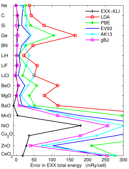
Figure 1: Error (in mRy/cell) in the EXX total energy calculated with orbitals generated from approximate exchange potentials with respect to the values obtained with the EXX-OEP orbitals.

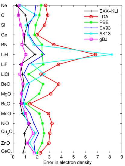
Figure 2: Integrated density difference as defined by Eq. (4).

We begin the discussion of the results with the EXX total energy $E_{\text{tot}}^{\text{EXX}}$. The results are shown graphically in Fig. 1 for each solid (see Table S2 of the Supplemental MaterialSM_ for the numerical values) and Table 1 contains the mean error (ME) and mean absolute error (MAE). As in Refs. Tran et al., 2015a, b, the EXX total energy expression [Eq. (1) for $E_{\text{x}}$ and no correlation] has been evaluated with the orbitals generated from various potentials. The error is with respect to the value obtained with the EXX-OEP orbitals: $E_{\text{tot}}^{\text{EXX}}[\{\psi_{i}^{\text{approx}}\}]-E_{\text{tot}}^{\text{EXX}}[\{\psi_{i}^{\text{EXX-OEP}}\}]$, where $E_{\text{tot}}^{\text{EXX}}[\{\psi_{i}^{\text{EXX-OEP}}\}]$ is the EXX total energy calculated with the EXX-OEP orbitals and $E_{\text{tot}}^{\text{EXX}}[\{\psi_{i}^{\text{approx}}\}]$ is the value obtained with orbitals obtained by one of the approximate exchange potentials. From the results we can see that the smallest errors with respect to EXX-OEP are obtained with the EXX-KLI and gBJ orbitals. With the exception of NiO, EXX-KLI leads to errors which are below 50 mRy/cell, and the MAE is about 20 mRy/cell. gBJ leads to very similar errors except for the transition-metal oxides and CeO₂ for which the errors are clearly larger (up to $\sim 260$ mRy/cell for NiO and CeO₂). These differences between the EXX-KLI and gBJ total energies for the transition-metal oxides are in line with the results for the electronic structure which show that EXX-KLI is much more accurate than gBJ (see below). The MAE with the gBJ potential of 55 mRy/cell is three times larger than for EXX-KLI. The orbitals generated by the other potentials lead to EXX total energies that are much higher (i.e., less negative) and to MAE of 218 (LDA), 139 (PBE), 87 (EV93), and 84 (AK13) mRy/cell. As a technical note, we remark that a few of the errors in Fig. 1 (Table S2) obtained with EXX-KLI and gBJ are slightly negative. In principle this should not occur, since among all sets of orbitals generated by a multiplicative potential, the EXX-OEP orbitals should, by definition, lead to the most negative EXX total energy. These negative values, which are anyway tiny and of no importance for the discussion, might be due to some minor (but unavoidable) incompatibilities between the two LAPW codes, e.g., details of the basis set or the integration methods.

Using the EXX total energy is a way to quantify with a single number the difference in shape between two sets of orbitals. An alternative is to consider the difference between the electron densities as follows:

$$\frac{100}{N}\int\limits_{\Omega}\left|\rho^{\text{approx}}(\bm{r})-\rho^{\text{EXX-OEP}}(\bm{r})\right|d^{3}r,$$ (4)

where $N=\int_{\Omega}\rho d^{3}r$ is the number of electrons in the unit cell $\Omega$ and the multiplication by 100 makes the numerical values more convenient. The absolute value of the integrand is taken in order to avoid cancellation between positive and negative values of $\rho^{\text{approx}}-\rho^{\text{EXX-OEP}}$. The results of Eq. (4) for the different approximate potentials and solids are displayed in Fig. 2, while The ME over the solids is shown in Table 1. The main observation is the same as with the EXX total energy, namely, the EXX-KLI and gBJ potentials lead to the smallest errors on average. However, both potentials lead to the same ME (0.9), which was not the case for the EXX total energy; one of the reasons is that Eq. (4) is normalized with the number of electrons that is much larger for the transition-metal oxides and CeO₂, such that the large spreads in the errors observed in Fig. 1 become similar to the other solids. This is again with LDA that the largest ME (3.1) is obtained. From Fig. 2 we can see that the LDA and AK13 potentials lead to very large density difference for LiH, which should mainly be due to the Li-$1s$ core states (see Sec. III.2).

Thus, we can conclude that in terms of EXX total energy and integrated electron density difference, the EXX-KLI and gBJ potentials are on average the closest to the EXX-OEP.

III.2 Electronic properties

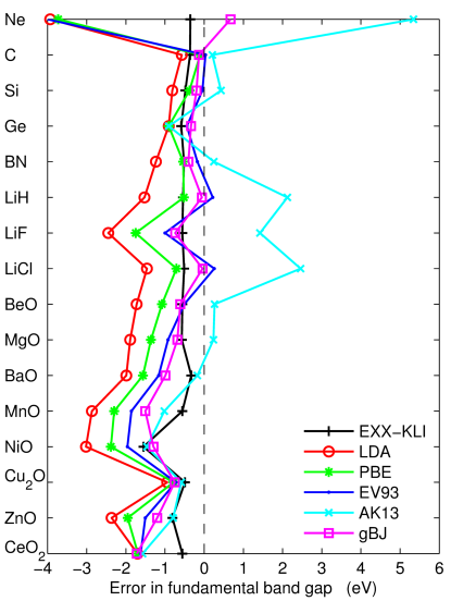
Figure 3: Error (in eV) in the KS fundamental band gap calculated with approximate exchange potentials with respect to the EXX-OEP values.

Turning now to the electronic band structure, the results for the KS fundamental band gap, defined as the conduction band minimum minus the valence band maximum, are shown in Fig. 3 and Table S3 of the Supplemental Material.SM_ The LDA and standard GGAs like PBE are known to underestimate the band gap by a rather large amount in solids compared to EXX-OEP.Städele et al. (1997); Betzinger et al. (2011); Hollins et al. (2012); Tran et al. (2015a); Engel (2016) Such an underestimation is indeed observed for all solids considered in the present work, and it is the largest, between 2 and 4 eV, for Ne, LiF, MnO, NiO, and ZnO. The GGA EV93 exchange functional,Engel and Vosko (1993) which was designed to have a functional derivative which resembles the EXX-OEP in atoms, increases the band gap with respect to the LDA and standard GGAs potentials such that a better agreement with EXX-OEP is usually obtained (see Fig. 3 and, e.g., Refs. Dufek et al., 1994; Tran et al., 2007, 2015a, 2015b). An exception is Ne since the EV93 band gap is slightly smaller than the LDA and PBE band gaps. In Table 1, the ME and MAE for the band gap are reduced for EV93 compared to LDA and PBE, but there is still a non-negligible underestimation of $-0.96$ eV on average. The AK13 potential also improves over LDA and PBE on average (ME and MAE of 0.39 and 1.20 eV, respectively), but leads to rather important overestimations for Ne, LiH, LiF, and LiCl, that are due to the excessively large positive values of the AK13 potential in the interstitial region as discussed in Refs. Tran et al., 2015a, b.

The smallest MAE in Table 1 for the band gap are obtained with the EXX-KLI and gBJ potentials, which lead to values in the range 0.6-0.7 eV, while the other potentials lead to MAE above 1 eV. Also, the error for Ne is strongly reduced compared to the other methods (see Fig. 3). However, by looking at the detailed results, we can see that there are some noticeable differences in the trends in the EXX-KLI and gBJ band gaps. In particular, the curve of the error for gBJ has a similar shape as for LDA, PBE, and EV93 in the sense that the error clearly varies from one solid to the other, while this is not the case with EXX-KLI since the error is in a narrow window around $-0.5$ eV for most solids except NiO ($-1.5$ eV). This is a quite interesting observation since the error in the band gap with EXX-KLI seems to be more predictable than with the other potentials. Direct comparisons between EXX-OEP and EXX-KLI were also reported by Engel and co-workers.Makmal et al. (2009); Engel and Schmid (2009) In Ref. Makmal et al., 2009, the EXX-KLI gap was reported to be too small in the CO and BeO molecules by 0.47 and 0.24 eV, respectively, while in Ref. Engel and Schmid, 2009 a metallic ground-state for antiferromagnetic FeO was obtained with EXX-KLI, which is a qualitatively wrong result since EXX-OEP (with LDA correlation added) leads to a band gap of 1.66 eV.Engel and Schmid (2009) Actually, we could confirm (with our implementation) that EXX-KLI leads to no band gap in FeO, which means that in this respect, semilocal potentials can perform better since gBJ (with 0.62 eV) and some othersTran et al. (2015b) open a band gap. We also mention that for CoO, we obtained a EXX-KLI band gap of 0.48 eV, which is about 2 eV smaller than the EXX-OEP value reported by Engel,Engel and Schmid (2009) while AK13 and gBJ lead to band gaps of 1.37 and 1.18 eV, respectively.

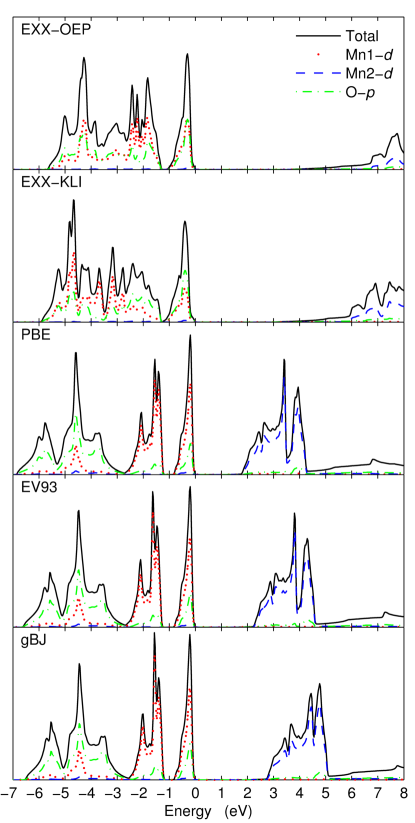
Figure 4: Spin-up DOS of MnO. Mn1 is the Mn atom with majority spin-up electrons. The Fermi energy is set at zero.

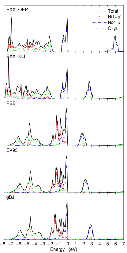
Figure 5: Spin-up DOS of NiO. Ni1 is the Ni atom with majority spin-up electrons. The Fermi energy is set at zero.

Besides the KS fundamental band gap, it may also be interesting to look at the density of states (DOS), in particular for the transition-metal oxides since qualitative differences in the occupied DOS can be observed. For the other solids, the visible difference in the DOS consists only of a change in the band gap, i.e., a rigid shift of the unoccupied states with respect to the occupied ones. The DOS of antiferromagnetic MnO and NiO are shown in Figs. 4 and 5, respectively. In MnO, the configuration of the $3d$-electrons on the Mn atom with majority spin-up electrons is $(t_{2g}^{\uparrow})^{3}(e_{g}^{\uparrow})^{2}(t_{2g}^{\downarrow})^{0}(e_{g}^{\downarrow})^{0}$ such that the band gap is determined mainly by the exchange splitting. The EXX-OEP DOS seems overall to be reproduced more accurately by the EXX-KLI potential. This is clearly the case for the DOS just below the Fermi energy and the unoccupied DOS, and actually, the EXX-OEP and EXX-KLI methods describe MnO as an insulator with a band gap of mixed Mott-Hubbard/charge-transfer type, while the band gap obtained by the other methods is much more of Mott-Hubbard type. However, in the energy range between 1 and 7 eV below the Fermi energy, noticeable differences between EXX-OEP and EXX-KLI can be observed, like for instance the Mn-$3d$ states at $-2$ eV in the EXX-OEP DOS that are shifted 1 or 2 eV deeper in energy by EXX-KLI.

In NiO, the electronic configuration is $(t_{2g}^{\uparrow})^{3}(e_{g}^{\uparrow})^{2}(t_{2g}^{\downarrow})^{3}(e_{g}^{\downarrow})^{0}$, which means a band gap that is determined mainly by the splitting between the $t_{2g}$ and $e_{g}$ states of the minority spin. Figure 5 shows that the agreement between EXX-OEP and EXX-KLI for the DOS is excellent, except for the position of the unoccupied states. As already observed in Ref. Tran et al., 2015a, all semilocal potentials (including the parameterization of gBJ specific for NiO, see Fig. 5 of Ref. Tran et al., 2015a) lead to DOS which differ significantly from the EXX-OEP DOS, like showing no sharp Ni-$3d$ peak at the lower part of the valence band or no clear energy separation between the spin-up and spin-down occupied Ni-$3d$ states. This is not the case with EXX-KLI, which reproduces accurately all features in the occupied EXX-OEP DOS. For the other transition-metal oxides Cu₂O and ZnO, the conclusion that the EXX-KLI DOS is the closest to the EXX-OEP remains also valid.

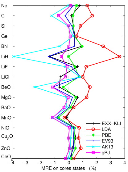
Figure 6: MRE (with respect to EXX-OEP and in %) for the energy position of the core states with respect to the VBM. For a given solid, the MRE is over all core states indicated in Table S1 (for LiH, the Li-$1s$ state was considered for the present analysis).

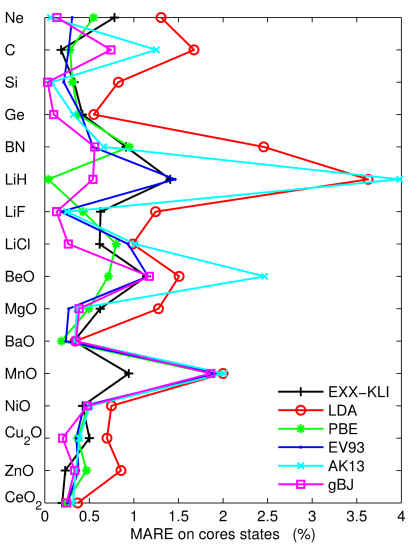
Figure 7: MARE (with respect to EXX-OEP and in %) for the energy position of the core states with respect to the VBM. For a given solid, the MARE is over all core states indicated in Table S1 (for LiH, the Li-$1s$ state was considered for the present analysis).

The results for the energy position of the core states with respect to the valence band maximum (VBM) are shown in Figs. 6 and 7. For a given solid and approximate potential, the MRE and MARE (in %) are defined as

$$\frac{100}{N_{\text{core}}}\sum_{i=1}^{N_{\text{core}}}\left(\Delta\varepsilon_{\text{core},i}^{\text{approx}}-\Delta\varepsilon_{\text{core},i}^{\text{EXX-OEP}}\right)/\left|\Delta\varepsilon_{\text{core},i}^{\text{EXX-OEP}}\right|$$ (5)

and

$$\frac{100}{N_{\text{core}}}\sum_{i=1}^{N_{\text{core}}}\left|\Delta\varepsilon_{\text{core},i}^{\text{approx}}-\Delta\varepsilon_{\text{core},i}^{\text{EXX-OEP}}\right|/\left|\Delta\varepsilon_{\text{core},i}^{\text{EXX-OEP}}\right|,$$ (6)

respectively, where the sum runs over the $N_{\text{core}}$ core states (see Table S1) and $\Delta\varepsilon_{\text{core},i}$ is the position of the $i$th core state with respect to the VBM. A negative MRE indicates that on average the core states are deeper in energy with the approximate potential than with EXX-OEP. The main observations are the following. On average, LDA and AK13 lead to too shallow and too deep core states, respectively, since their mean MRE (MMRE, see Table 1) are 1.1% and $-0.6\%$. The other exchange potentials are more accurate and lead to rather similar values with a MMRE below 0.3% in magnitude, and a mean MARE (MMARE) that is in the range 0.5-0.6%.

III.3 Magnetic moment and EFG

Table 2: Atomic spin magnetic moment $\mu_{S}$ (in $\mu_{\text{B}}$) in MnO and NiO and EFG (in $10^{21}$ V/m²) at the Cu site in Cu₂O calculated from different exchange potentials.

Potential	$\mu_{S}^{\text{Mn}}$	$\mu_{S}^{\text{Ni}}$	EFG${}_{\text{Cu}}$
EXX-OEP	4.59	1.91	-17.7
EXX-KLI	4.58	1.79	-11.1
LDA	4.18	1.30	-4.7
PBE	4.23	1.43	-5.6
EV93	4.30	1.51	-6.8
AK13	4.39	1.58	-8.1
gBJ	4.35	1.61	-7.0
HF	4.57	1.88	-17.0

We continue the discussion of the results with the atomic spin magnetic moment $\mu_{S}$ in MnO and NiO and the EFG in Cu₂O. The results in Table 2 show that EXX-KLI is a very good approximation to EXX-OEP for $\mu_{S}$ since the values obtained with the two methods differ by only $\sim 0.1$ $\mu_{\text{B}}$ for NiO and are the same for MnO. The other exchange potentials lead to substantially smaller values. We note that in our previous work,Tran et al. (2015a) a value of 1.86 $\mu_{\text{B}}$ for NiO could be obtained with gBJ, but with parameters $(\gamma,c,p)$ that were tuned specifically for NiO. The EFG at the Cu site in Cu₂O has a value of $-17.7\times 10^{21}$ V/m² with EXX-OEP, but is substantially smaller with all other potentials including EXX-KLI which leads to the best agreement with $-11.1\times 10^{21}$ V/m² ($\sim 40\%$ too small). As for NiO, we could find a parameterization of a modified form of the gBJ potential (see Ref. Tran et al., 2015a for details) that leads to an EFG approaching the EXX-OEP value.

In addition to the results obtained with the multiplicative exchange potentials, the HF values are also reported in Table 2, and as already noticed in Ref. Tran et al., 2015a, the EXX-OEP and HF methods provide basically the same values. This is expected for such properties calculated from the electron density, since the two methods should in principle lead to electron densities that should not differ up to the first order, Krieger et al. (1992b); Grabo et al. (2000); Kümmel and Perdew (2003b) despite completely different electronic structures.Tran et al. (2015a)

III.4 Further discussion

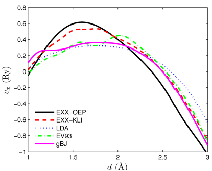
Figure 8: Exchange potentials $v_{\text{x}}$ in Cu₂O plotted starting at a distance of 1 Å from the Cu atom at site $\left(1/2,1/2,0\right)$ ($d=0$) in the direction of the O atom at site $\left(3/4,3/4,3/4\right)$ ($d=3.54$ Å).

In our previous works about exchange potentials in solids Tran et al. (2007); Betzinger et al. (2011); Koller et al. (2011); Tran et al. (2015a, b) as well as in Refs. Städele et al., 1997, 1999; Aulbur et al., 2000; Qteish et al., 2006, a rather clear understanding of the results could be achieved by visualizing the potential and electron density. For instance, in solids where the VBM and conduction band minimum (CBM) are located in different regions of space (typically, the VBM is localized around atoms and the CBM in the interstitial region), the size of the band gap is directly related to the value of the potential in the two regions. The more the values of the potential in the two regions differ, the more the band gap should be large (see Ref. Tran et al., 2007 for LiCl and Ref. Tran et al., 2015b for Kr and BaO). The situation may be different in transition-metal oxides where the band gap can be of on-site $d$-$d$ type such that, for instance, it is determined by the splitting between occupied and unoccupied $d$-states. In such cases like Cu₂OKoller et al. (2011) or NiO,Tran et al. (2015a, b) the size of the band gap and atomic magnetic moment are determined by the sensitivity of the potential to the $d$-orbital shape (e.g., $t_{2g}$ versus $e_{g}$) and/or the magnitude of $v_{\text{x},\uparrow}-v_{\text{x},\downarrow}$. In Ref. Tran et al., 2015a it was also shown that the differences between the electron densities generated by the various potentials correlate quite well with the numerical results for the total energy, magnetic moment, etc.

From these analyses it was concluded that the LDA and standard GGA potentials like PBE are much more homogeneous than the EXX-OEP,Tran et al. (2015a) explaining why they lead to band gap and magnetic moment that are much smaller than with EXX-OEP. The more specialized potentials EV93, AK13, and gBJ are more inhomogeneous such that they are better approximations to the EXX-OEP. This is particularly the case for the gBJ potential which was shown to reproduce quite accurately most features of the EXX-OEP, provided that the appropriate parameters $\gamma$, $c$, and $p$ are used. The same analysis can also be made for the results obtained in the present work. However, since the observations and conclusions would be very similar to those obtained in our previous works, only a brief discussion for two of the most interesting systems, Cu₂O and NiO, is given.

Figure 8 shows exchange potentials in Cu₂O plotted along a portion of the path between the Cu and O atoms located at sites $\left(1/2,1/2,0\right)$ and $\left(3/4,3/4,3/4\right)$ of the unit cell, respectively. In Refs. Tran et al., 2015a, b, we identified a (valence) region close to the Cu atom ($1\lesssim d\lesssim 2$ Å) to be important for the band gap and EFG, since it was observed that the potentials which agree with the EXX-OEP in this region in particular, namely, gBJ with the universal correction, Becke-Roussel,Becke (1988) and Slater, lead to reasonable values for the band gap and EFG. To some extent the same is true for the EXX-KLI potential, since from Fig. 8 we can see that it is relatively close to EXX-OEP compared to the other potentials [see Fig. 8(b) of Ref. Tran et al., 2015a and Fig. 3 of Ref. Tran et al., 2015b for more potentials] and also leads to smaller difference with respect to EXX-OEP for the band gap and EFG as discussed above.

Figure 9: Two-dimensional plots of $v_{\text{x}}^{\uparrow}-v_{\text{x}}^{\downarrow}$ in a $(001)$ plane of antiferromagnetic NiO. The contour lines start at $-2$ Ry (blue color) and end at 2 Ry (red color) with an interval of 0.235 Ry. The Ni atom with a full spin-up $3d$-shell is at the left upper corner.

The difference $v_{\text{x}}^{\uparrow}-v_{\text{x}}^{\downarrow}$ between the spin-up and spin-down exchange potentials for antiferromagnetic NiO in a (001) plane is shown in Fig. 9. As we can observe (see Fig. 10 of Ref. Tran et al., 2015a and Fig. 4 of Ref. Tran et al., 2015b for other potentials) the shape of the unoccupied $e_{g}$ orbitals is the most pronounced with EXX-OEP and all semilocal potentials (except gBJ with parameters for NiOTran et al. (2015a)) lead to a $e_{g}$-shape that is very much attenuated with respect to EXX-OEP. Compared to the semilocal potentials, EXX-KLI seems to be more accurate, however the magnitude of $v_{\text{x}}^{\uparrow}-v_{\text{x}}^{\downarrow}$ is still too small, thus explaining the underestimation of the magnetic moment and band gap.

More generally, since the EXX-KLI potential is derived from the EXX-OEP by using the closure approximation (i.e., directional averaging), it is expected to be smoother than the EXX-OEP. This has been underlined by Engel and co-workers in Refs. Engel and Schmid, 2009; Engel and Dreizler, 2011 who already showed that for Si and FeO the EXX-KLI potential around the atoms is less aspherical than the EXX-OEP. Thus, for systems with a highly aspherical electron density, e.g., systems with an open $3d$-shell, the closure approximation should have a large impact on the results. This is what has indeed been observed for FeO (metallic with EXX-KLI but not with EXX-OEPEngel and Schmid (2009)) and NiO (much larger underestimation of the band gap than for the other solids, see Fig. 3). In comparison, the electron density on the Mn atom in MnO is more spherical (the $3d$-shell is full for one spin and empty for the other spin), therefore the underestimation of the band gap is not as large, but similar as for the non-magnetic solids.

IV Summary and conclusion

In this work, we have presented the results of electronic structure calculations on solids with the EXX-KLI approximation to the exact exchange potential EXX-OEP. The goals were to provide all-electron benchmark EXX-KLI (and new EXX-OEP) results and to figure out if EXX-KLI can be used safely as a substitute to EXX-OEP, and if it is more accurate than the semilocal approximations like the MGGA gBJ potential. The test set consisted of 16 solids of various types and the calculated properties were the EXX total energy, electron density, electronic structure, magnetic moment, and EFG.

The results for the total energy and electronic structure have shown that on average the EXX-KLI and gBJ approximations are more or less of the same accuracy. However, by looking at the results in more detail we have noticed that for the transition-metal oxides, the EXX-KLI and gBJ results can differ qualitatively. For instance, opposite trends were observed for the band gap in the antiferromagnetic systems; while EXX-KLI leads to a fairly accurate band gap in MnO (clearly more accurate than gBJ), it is by far too small or even zero for NiO, CoO, and FeO (gBJ is better than EXX-KLI for these cases). The EXX-KLI approximation seems to be quite inaccurate in the case of highly aspherical electron density like in NiO, FeO, and CoO as noticed previously.Engel and Schmid (2009) On the other hand, the EXX-OEP occupied DOS of MnO and NiO are reproduced accurately by EXX-KLI, while all semilocal potentials lead to completely different DOS, especially for NiO. The other difference between EXX-KLI and gBJ is the error for the band gap: with EXX-KLI there is a systematic underestimation of the order of $\sim 0.5$ eV for all systems except NiO, while for gBJ and all other semilocal potentials the error varies strongly among the compounds.

For the magnetic moment and EFG, the EXX-OEP results are reproduced more accurately by EXX-KLI, nevertheless a clear underestimation of the magnitude of the EFG in Cu₂O is still observed.

Thus, in conclusion, EXX-KLI seems to be a rather good approximation to EXX-OEP for ground-state properties, i.e., properties which are calculated using the occupied orbitals. For the band gap, an excited-state property, EXX-KLI leads to an underestimation of $\sim 0.5$ eV for most systems, except in the special case of antiferromagnetic NiO (and also FeO and CoO) for which a much larger error of more than 1.5 eV is obtained. The results obtained with gBJ, the most accurate of the tested semilocal potentials, are also rather good, but more unpredictable for the band gap, a behavior which is in general more expected for semilocal approximations than for ab initio approximations like EXX-KLI.

Concerning the LHF/CEDADella Sala and Görling (2001); Gritsenko and Baerends (2001) method briefly mentioned in Sec. II, which, in principle, should be a better approximation to EXX-OEP (but also more expensive) than KLI, the works published so farDella Sala and Görling (2001); Grüning et al. (2002) have shown that the LHF/CEDA and KLI results for the total energy and gap are quasi-identical in most cases (see also Ref. Kümmel and Kronik, 2008 for further discussion). However, since these LHF/CEDA calculations were done for atoms and light molecules, it is not certain that this conclusion would hold also for much more complicated systems like NiO or FeO.