Hydrodynamic VS collisionless dynamics of a 1D harmonically trapped Bose gas

Abstract

By using a sum rule approach we investigate the transition between the hydrodynamic and the collisionless regime of the collective modes in a 1D harmonically trapped Bose gas. Both the weakly interacting gas and the Tonks-Girardeau limits are considered. We predict that the excitation of the dipole compression mode is characterized, in the high temperature collisionless regime, by a beating signal of two different frequencies ($\omega_{z}$ and $3\omega_{z}$) while, in the high temperature collisional regime, the excitation consists of a single frequency ($\sqrt{7}\omega_{z}$). This behaviour differs from the case of the lowest breathing mode whose excitation consists of a single frequency ($2\omega_{z}$) in both regimes. Our predictions for the dipole compression mode open promising perspectives for the experimental investigation of collisional effects in 1D configurations.

I Introduction

Thermalization and relaxation phenomena represent a key issue in one-dimensional (1D) systems Popov2001 ; Giamarchi2004 of identical bosons with zero–range repulsive interaction due to the intrinsic integrability Thacker1981 ; Yurovsky2008 ; Rigol2007 of this many-body system and have been the object of recent experimental and theoretical investigations Kinoshita2006 ; Hofferberth2007 ; Hofferberth2008 ; vanAmerongen2008 ; Mazets2008 ; Mazets2009 ; Tan2010 ; Laburthe Tolra2004 . They play an important role not only for the achievement of equilibrium but also for the propagation of collective modes Mazets2011 whose nature, in harmonically trapped configurations, is expected to evolve from the hydrodynamic regime (HD) at low temperature to a collisionless (CL) regime at higher temperature. At low temperature, the applicability of the hydrodynamic description is ensured by the phononic nature of the elementary excitations. Phonons are in fact known to characterize the long wavelength dispersion of the excitation spectrum in one-dimensional interacting Bose gases Lieb1963 and their description has the same form as the one given by the hydrodynamic theory of superfluids Menotti2002 ; DeRosi2015 . At high temperature highT , due to the exponential decrease of the density caused by harmonic trapping, collisions become rare and the system enters the collisionless regime described by the ideal gas model. One then expects a transition between the two regimes which could provide valuable informations on the collisional effects in 1D configurations.

So far most of the attention in the collective features of 1D harmonically trapped Bose gases has concerned the lowest breathing (LB) mode. The frequency of this mode was calculated at T=0 within the Lieb-Liniger model using a sum rule approach Menotti2002 , exploring the transition from the weakly interacting Bogoliubov gas (BG) to the Tonks-Girardeau (TG) limit of strongly repulsive bosons Tonks1936 ; Girardeau1960 . The experimental results of Haller2009 have confirmed with good accuracy the predictions of theory. Recent studies of this mode have also focused on the so called super-Tonks-Girardeau (STG) regime of hard rods Astrakharchik2005 ; Haller2009 and on the regime of small number of particles (or small coupling constant $g_{1D}$) where the Local Density Approximation (LDA), usually employed to calculate the density profiles using the equation of state of uniform matter, is not applicable Gudyma2015 ; Chen2015 ; Gudyma20152 . The temperature dependence of the frequency of the lowest breathing mode has also been the object of recent theoretical Hu2014 ; Chen2015 and experimental Moritz2003 ; Fang2014 work. The theoretical predictions are usually based on a hydrodynamic description where the relevant thermodynamic quantities are calculated using the Yang-Yang theory Yang1969 , which generalizes the Lieb-Liniger theory Lieb1963 of interacting 1D bosons to finite temperature. A characteristic feature of the hydrodynamic theory applied to the lowest breathing mode is that, at high temperatures, it predicts Fang2014 ; Hu2014 ; DeRosi2015 the same frequency $\omega=2\omega_{z}$ as given by the non interacting gas model, see Table 1. This rules out the possibility of a simple identification of the hydrodynamic VS the collisionless nature of the oscillation.

In this work we exploit the different behaviour exhibited by the dipole compression (DC) mode, identified as the lowest compression mode with the same parity as the center of mass (dipole) mode. Differently from the center of mass mode, which oscillates with the model independent frequency $\omega=\omega_{z}$, the dipole compression mode is sensitive to the equation of state and, differently from the lowest breathing mode, is characterized by a different excitation spectrum at high temperatures, when investigated in the hydrodynamic or in the collisionless regimes, see Table 2. This mode, whose frequency has been already measured at low temperature in elongated configurations in the case of the unitary Fermi gas Tey2013 , is consequently a natural candidate to exploit the effects of relaxation caused by collisions and the corresponding thermalization effects in 1D configurations. Numerical calculations for the DC frequencies at zero and finite temperature in the hydrodynamic framework have been carried out in Hu2014 .

In the following we will use the Lieb-Liniger Hamiltonian Kheruntsyan2005

$$H=H_{kin}+H_{int}+H_{trap}=\\ =-\frac{\hbar^{2}}{2m}\sum_{i=1}^{N}\frac{\partial^{2}}{\partial z_{i}^{2}}+g_{1D}\sum_{i>j}^{N}\delta(z_{ij})+\sum_{i=1}^{N}V_{ext}(z_{i})\ ,$$ (1)

describing a gas of 1D interacting Bose particles in the presence of the harmonic potential $V_{ext}(z)=m\omega_{z}^{2}z^{2}/2$. Here $z_{ij}\equiv z_{i}-z_{j}$ is the relative coordinate and $g_{1D}$ is the relevant 1D coupling constant. In the presence of radial harmonic trapping and in the absence of confinement induced resonance Olshanii1998 ; Petrov2000 , the interaction parameter $g_{1D}$ can be written as $g_{1D}=2\hbar^{2}a/ma^{2}_{\perp}$ where $a$ is the three-dimensional scattering length and $a_{\perp}$ is the radial oscillator length.

Our paper is organized as follows.

In Section II we summarize the basic results of hydrodynamic theory of 1D gases confined by a harmonic potential. This theory allows for analytic results for the collective frequencies if the equation of state exhibits a polytropic dependence on the density DeRosi2015 . Furthermore it can be conveniently formulated using a variational procedure allowing for an easy determination of the collective frequencies in the intermediate regimes of temperature and interaction.

In Section III we formulate a sum rule approach to describe the frequency of the collective oscillations in the presence of harmonic trapping. This approach provides a useful insight on the physical features of the collective oscillations, both at zero and finite temperature. In this Section we will also provide a valuable derivation of the 1D virial theorem, holding in all regimes of temperature and interaction. An extension of the virial theorem, which turns out to be useful for the study of the dipole compression mode, will be also presented.

In Section IV we discuss the dipole compression frequency and point out the different behaviour exhibited in the hydrodynamic and in the collisionless regime of high temperature. In particular, in the latter case, this mode exhibits a characteristic beating effect involving two different frequencies which are expected to be of easy experimental identification.

In Section V we draw our final conclusions.

II Hydrodynamic theory of 1D Bose gases in the presence of harmonic trapping

We consider the 1D version

$$m(\omega^{2}-\omega^{2}_{z})nv+\frac{\partial}{\partial z}\left[n\left(\frac{\partial P}{\partial n}\right)_{\bar{s}}\frac{\partial v}{\partial z}\right]=0$$ (2)

of the linearized hydrodynamic equation Griffin1997 ; Taylor2009 ; DeRosi2015 for the velocity field $v(z)$, where $(\partial P/\partial n)_{\bar{s}}$ is the adiabatic compressibility ($\bar{s}$ being the entropy per particle) evaluated at the local value of the 1D equilibrium density profile $n\equiv n(z)$ whose $z$-dependence, caused by the external potentials $V_{ext}(z)$, can be determined in the Local Density Approximation, through the solution of the equilibrium Euler equation

$$\left(\frac{\partial P(z)}{\partial n}\right)_{T}\frac{\partial n(z)}{\partial z}+n(z)\frac{\partial V_{ext}(z)}{\partial z}=0\ ,$$ (3)

for a fixed value of the temperature of the gas.

The above equations show that the eigenfrequencies $\omega$ of the collective oscillations are determined once the adiabatic and the isothermal $(\partial P/\partial n)_{T}$ compressibilities, calculated at the local value $n(z)$ of the density, are known. These quantities depend on the interaction and on the temperature of the gas.

In the uniform case ($V_{ext}=0$) Eq. (2) admits a plane wave solution $v\propto e^{iqz}$ yielding the phonon dispersion relation $\omega=c_{s}q$, where $c_{s}=\sqrt{(\partial P/\partial n)_{\bar{s}}/m}$ is the adiabatic sound velocity.

It is worth noticing that, since in 1D there is no superfluid phase transition Mermin1966 ; Hohenberg1967 , Eq. (2) can be applied to all temperatures provided the dynamic behaviour of the gas is correctly described by hydrodynamic theory. This represents an important difference with respect to 2D and 3D systems where hydrodynamic theory, for temperatures below the critical value, should be generalized to the Landau theory of two fluids Pitaevskii2016 .

It is immediate to show that Eq. (2) can be derived Hou2013 from the variational approach $\delta\omega^{2}/\delta v=0$ , with

$$\omega^{2}=\omega_{z}^{2}+\frac{\int dzn\left(\frac{\partial P}{\partial n}\right)_{\bar{s}}\left(\frac{\partial v}{\partial z}\right)^{2}}{\int dzmnv^{2}}\ ,$$ (4)

first developed in 3D systems Taylor2005 ; Taylor2008 ; Taylor2009 . The advantage of using the variational approach, Eq. (4), rather than the differential hydrodynamic equation, Eq. (2), is that one can easily estimate the collective frequencies, at zero as well as at finite temperature, with a suitable ansatz for the velocity field. This method has been recently implemented in Hu2014 .

In addition to the universal dipole result $\omega(D)=\omega_{z}$ for the center of mass oscillation (Kohn mode), corresponding to the choice $v=const$, useful expressions for the frequencies of the relevant collective modes concern the lowest breathing mode

$$\omega^{2}_{HD}(LB)=\omega_{z}^{2}+\frac{\int dzn\left(\frac{\partial P}{\partial n}\right)_{\bar{s}}}{\int dzmnz^{2}}\ ,$$ (5)

corresponding to the ansatz $v=z$, and the dipole compression mode

$$\omega^{2}_{HD}(DC)=\omega_{z}^{2}+\frac{\int dzn\left(\frac{\partial P}{\partial n}\right)_{\bar{s}}4z^{2}}{\int dzmn(z^{2}-\langle z^{2}\rangle)^{2}}\ ,$$ (6)

corresponding to the ansatz $v=z^{2}-\langle z^{2}\rangle$ where $\langle z^{2}\rangle$ is the average value of $z^{2}$ calculated at equilibrium. The term $\langle z^{2}\rangle$ ensures the orthogonality between the dipole compression mode and the center of mass oscillation. This is easily proven by noticing that the density variations $\partial_{z}[vn]$ associated with the DC mode give rise to a vanishing dipole moment: $\int dzz\partial_{z}[vn]=0$.

Predictions (5) and (6) for the lowest breathing and the dipole compression modes are expected to provide an accurate approximation to the exact solutions of the hydrodynamic equation (2) in all regimes of interaction and temperature. This is the consequence of the fact that the corresponding ansatz for the velocity field coincides with the exact solution of the hydrodynamic equation in important asymptotic regimes, where the equation of state exhibits a polytropic dependence on the density DeRosi2015 , like the $T=0$ weakly interacting limit, the $T=0$ Tonks-Girardeau limit as well as in the classical regime of high temperatures highT ; DeRosi2015 . One then expects that the same ansatz for $v$ will be accurate also in the intermediate regimes of interaction and temperature. Such an accuracy was recently proven numerically by Hu et al. Hu2014 . The values of the hydrodynamic frequencies calculated in the above three asymptotic regimes DeRosi2015 are reported in Table 1 for the lowest breathing mode and in Table 2 for the dipole compressional mode. Finally, we notice that the LB HD frequencies of Table 1 were obtained also by Bouchoule et al. Bouchoule2016 using scaling arguments starting from the HD equations.

Table 1: Hydrodynamic VS collisionless frequencies of the lowest breathing mode ($LB$) for a 1D Bose gas.

	Hydrodynamic
	T = 0	high T	Collisionless
1D weakly interact. (BG)	$\sqrt{3}\omega_{z}$	$2\omega_{z}$	$2\omega_{z}$
1D Tonks-Girardeau	$2\omega_{z}$	$2\omega_{z}$	$2\omega_{z}$

Table 2: Hydrodynamic VS collisionless frequencies of the dipole compressional mode ($DC$) for a 1D Bose gas.

	Hydrodynamic
	T = 0	high T	Collisionless
1D weakly interact. (BG)	$\sqrt{6}\omega_{z}$	$\sqrt{7}\omega_{z}$	$3\omega_{z}\hskip 2.84544pt\&\hskip 2.84544pt1\omega_{z}$
1D Tonks-Girardeau	$3\omega_{z}$	$\sqrt{7}\omega_{z}$	$3\omega_{z}\hskip 2.84544pt\&\hskip 2.84544pt1\omega_{z}$

III Sum rules and collective oscillations

Sum rules represent a powerful tool to describe the collective behaviour exhibited by quantum many-body systems Lipparini1989 ; Stringari1996 ; Pitaevskii2016 . Their main merit is that, in many cases, they provide accurate predictions for the collective frequencies avoiding the full solution of the quantum many-body problem. Furthermore, being based on the algebra of commutators, they emphasize the symmetry properties of the problem and the role of conservation rules. In general sum rules provide compact expressions for the $p$-moments

$$m_{p}(F)=\hbar\int_{-\infty}^{+\infty}(\hbar\omega)^{p}S_{F}(\omega)d\omega$$ (7)

of the dynamic structure factor

$$S_{F}(\omega)=Q^{-1}\sum_{n,m=1}^{N}e^{-\beta E_{m}}|\bra{m}F\ket{n}|^{2}\delta(\hbar\omega-\hbar\omega_{nm})\ ,$$ (8)

where $F=\sum_{k=1}^{N}f(z_{k})$ is the relevant excitation operator, $Q=\sum_{m=1}^{N}\exp[-\beta E_{m}]$ is the partition function and $\omega_{nm}=(E_{n}-E_{m})/\hbar$ are the Bohr transition frequencies, relative to the Hamiltonian, Eq. (1).

An important sum rule, widely employed in many-body calculations, concerns the inverse-energy weighted moment $m_{-1}$ of the dynamic structure factor. This moment is directly related to the static response $\chi(F)$ defined in terms of the fluctuation $\delta\langle F\rangle=\lambda\chi(F)$, induced by an external static perturbation of the form $H_{pert}=-\lambda F$ applied to the system, according to the relationship Pitaevskii2016 $\chi(F)=2m_{-1}(F)$.

The $m_{-1}$ sum rule can be combined with the energy weighted sum rule, which in general can be reduced in the form of a double commutator involving the Hamiltonian $H$ and the excitation operator $F$, yielding the simple result

$$m_{1}(F)=\frac{1}{2}\langle[F,[H,F]]\rangle=\frac{\hbar^{2}}{2m}N\langle|\nabla_{z}f(z)|^{2}\rangle\ ,$$ (9)

to provide an estimate of the collective frequency through the ratio

$$\hbar^{2}\omega^{2}_{1,-1}=\frac{m_{1}}{m_{-1}}\ .$$ (10)

In the presence of harmonic trapping, the choice for the excitation operator depends on the nature of the collective mode. For the lowest breathing mode the natural choice is provided by the operator $F_{LB}=\sum_{k=1}^{N}(z^{2}_{k}-\langle z^{2}\rangle)$ note v which ensures the condition $\langle F_{LB}\rangle=0$ at equilibrium. In this case the inverse energy weighted moment can be easily calculated since the static perturbation $-\lambda F_{LB}$ consists of a simple renormalization of the harmonic trapping frequency. One then obtains the following result Pitaevskii2016 ; Menotti2002

$$m_{-1}(LB)=-\frac{N}{m}\frac{\partial\langle z^{2}\rangle}{\partial\omega_{z}^{2}}\ ,$$ (11)

for the inverse energy weighted moment. On the other hand, the energy weighted moment (9), relative to the same excitation operator, yields the result

$$m_{1}(LB)=\frac{2N\hbar^{2}}{m}\langle z^{2}\rangle\ ,$$ (12)

so that the ratio between the two sum rules provides the expression

$$\omega^{2}_{1,-1}(LB)=-2\frac{\langle z^{2}\rangle}{\partial\langle z^{2}\rangle/\partial\omega_{z}^{2}}$$ (13)

for the squared collective frequency.

Result (13) was successfully employed to evaluate the LB frequency in 1D Bose gases at zero temperature Menotti2002 . In particular, by using the Local Density Approximation to evaluate the $\omega_{z}$-dependence of the average square radius, this equation accounts for the transition of the collective frequency from the value $\sqrt{3}\omega_{z}$ holding in the weakly interacting Bose gas to the value $2\omega_{z}$ holding in the Tonks-Girardeau limit, see Table 1. Since Eq. (13) does not assume the Local Density Approximation, it can be also used to estimate the collective frequencies when the coupling constant $g_{1D}$ or the number of atoms are small Gudyma2015 ; Gudyma20152 . One should however notice that result (13) is not adequate to describe the frequency of the LB mode at finite temperature. This is best understood in the classical limit of high temperatures where Eq. (13) provides the result $\sqrt{2}\omega_{z}$ for the collective frequency to be compared with the exact value $2\omega_{z}$ holding in the classical limit where the Hamiltonian of the system reduces to the ideal gas value (see Table 1). The discrepancy between the two values is due to the fact that, at finite temperature, the operator $F_{LB}$ excites zero frequency modes which provide a finite contribution to the inverse energy weighted moment sum rule uniform .

The correct value of the collective frequency at finite temperature is recovered if, instead of calculating the inverse energy weighted sum rule, one evaluates the cubic energy weighted sum rule $m_{3}(F)$ which can be written in the form of a double commutator involving the Hamiltonian $H$ and the commutator $[H,F]$:

$$m_{3}(F)=\frac{1}{2}\langle[[F,H],[H,[H,F]]]\rangle\ .$$ (14)

Differently from $m_{-1}(F)$, the cubic energy weighted moment is not sensitive to the zero frequency modes excited by the operator $F$ at high temperature. Evaluation of the triple commutator (14) with the Lieb-Liniger Hamiltonian (1) yields the following result for the $m_{3}$ sum rule relative to the excitation operator $F_{LB}=\sum_{k=1}^{N}(z^{2}_{k}-\langle z^{2}\rangle)$:

$$m_{3}(LB)=\frac{2\hbar^{4}}{m^{2}}\left(4\langle H_{kin}\rangle+4\langle H_{trap}\rangle+\langle H_{int}\rangle\right)\ .$$ (15)

A useful simplification of Eq. (15) is provided by the virial theorem Pitaevskii2016 ; Stringari1996 ; Gudyma20152 , which can be derived by imposing the general condition $\langle[H,G]\rangle=0$ holding at equilibrium for any choice of the operator $G$. By making the choice $G=\sum_{k=1}^{N}\left(z_{k}p_{z,k}+p_{z,k}z_{k}\right)$ corresponding to a scaling deformation of the many-body wave function, one derives the exact relationship

$$2\langle H_{kin}\rangle-2\langle H_{trap}\rangle+\langle H_{int}\rangle=0\ .$$ (16)

Thanks to the virial theorem (16) the cubic energy weighted sum rule (15) can be further simplified and, combined with the energy weighted sum rule (12), yields the following expression for the LB collective frequency Gudyma20152

$$\hbar^{2}\omega_{3,1}^{2}(LB)=\frac{m_{3}(LB)}{m_{1}(LB)}=\hbar^{2}\omega_{z}^{2}\left(4-\frac{\langle H_{int}\rangle}{2\langle H_{trap}\rangle}\right)\ ,$$ (17)

or, equivalently Gudyma20152 ,

$$\omega_{3,1}^{2}(LB)=\omega_{z}^{2}\left(3+\frac{\langle H_{kin}\rangle}{\langle H_{trap}\rangle}\right)\ ,$$ (18)

holding also beyond LDA. Eq. (17) explicitly shows that, if the average value of the interaction energy is negligible, as happens in the TG regime and in the collisionless regime of high temperatures, one recovers the correct value $2\omega_{z}$ for the lowest compression mode (see Table 1). In the case of the weakly interacting Bose gas one can neglect, at T=0, the kinetic energy term and Eq. (18) correctly reproduces the hydrodynamic value $\sqrt{3}\omega_{z}$. In conclusion one expects that the sum rule result $m_{3}/m_{1}$ will provide an excellent estimate of the frequency of the lowest compression mode in all ranges of temperature, interaction and number of particles. At $T=0$ it is expected to provide results of similar accuracy as prediction (13) based on the ratio between the energy weighted and inverse energy weighted sum rule. The expression (17) for the LB collective frequency was already considered by Fang et al. Fang2014 to analyze their experimental data at finite temperature.

A further interesting expression for the $\omega_{3,1}^{2}$ ratio can be obtained by using the Hellmann-Feynman expression $\langle H_{int}\rangle=g_{1D}\partial F/\partial g_{1D}$ for the interaction energy, where $F$ is the free energy of the system. In this way Eq. (17) takes the form

$$\omega_{3,1}^{2}(LB)=\omega_{z}^{2}\left[4+\frac{\hbar^{2}\mathcal{C}a_{1D}}{2m\langle H_{trap}\rangle}\right]$$ (19)

where we have introduced the 1D Tan’s contact parameter $\mathcal{C}=(m/\hbar^{2})\partial F/\partial a_{1D}$ with $a_{1D}=-2\hbar^{2}/mg_{1D}$ the 1D scattering length. The same result can be obtained by using the Tan’s contact 1D virial theorem (see, for example Valiente2012 ). The Tan’s contact, which characterizes the large momentum tail of the momentum distribution, can be also expressed in terms of the pair correlation function Gangardt2003 . Result (19) relates the frequency of the lowest compression modes, fixed with high accuracy by the ratio $\omega_{3,1}^{2}(LB)$, to independently measurable quantities.

A similar analysis can be worked out for the dipole compression mode excited by the operator $F_{DC}=\sum_{k=1}^{N}f_{DC}(z_{k})$ with $f_{DC}(z)=z^{3}/3-z\langle z^{2}\rangle$ note v . The choice ensures that the operator $F_{DC}$ will not excite the center of mass (dipole) oscillation. This can be easily shown by checking that the crossed energy weighted sum rule $\langle[F_{D},[H,F_{DC}]]\rangle$, with $F_{D}=\sum_{k=1}^{N}z_{k}$, identically vanishes.

In the case of the DC mode the static response, and hence the inverse energy weighted sum rule, can be easily calculated only in the LDA where, in the presence of the external perturbation $-\lambda F_{DC}$, the chemical potential is modified according to $\mu\to\mu-\lambda f_{DC}(z)$ and the density profile is, accordingly, modified as $n(z)\to n(z)+\lambda f_{DC}(z)(\partial n/\partial\mu)_{T}$. The inverse energy weighted sum rule relative to the DC mode then takes the useful form notedeltamu :

$$m_{-1}(DC)=\frac{1}{2}\int dz\left(\frac{z^{3}}{3}-z\langle z^{2}\rangle\right)^{2}\left(\frac{\partial n}{\partial\mu}\right)_{T}\ .$$ (20)

Using Eq. (9), the energy weighted moment is also easily evaluated and takes the form:

$$m_{1}(DC)=\frac{\hbar^{2}N}{2m}(\langle z^{4}\rangle-\langle z^{2}\rangle^{2})\ .$$ (21)

It is straightforward to verify that, at T=0, the ratio $m_{1}/m_{-1}$ provides the correct (squared) hydrodynamic frequencies both in the weakly interacting Bose gas ($\sqrt{6}\omega_{z}$), where $\partial\mu/\partial n=g_{1D}$, and in the Tonks-Girardeau limit ($3\omega_{z}$), where $\partial\mu/\partial n=\hbar^{2}\pi^{2}n/m$. At high temperatures, where $\partial\mu/\partial n_{|T}=\partial P/\partial n_{|T}/n=k_{B}T/n$, one instead finds that the frequency $\omega_{1,-1}$ takes the value $\sqrt{3}\omega_{z}$ which is smaller than the hydrodynamic value $\sqrt{7}\omega_{z}$, similarly to the case of the LB mode discussed above. This result is the consequence of the fact that the DC operator $F_{DC}$ excites, at high temperature, two modes with frequency equal to $\omega_{z}$ and $3\omega_{z}$, respectively. The corresponding strengths $\sigma_{1}$ and $\sigma_{3}$ characterizing the dynamic structure factor $S_{F}(\omega)$ can be easily evaluated through the identification

$$\omega_{1,-1}^{2}(DC)=\frac{\sigma_{1}\omega_{z}+3\sigma_{3}\omega_{z}}{\sigma_{1}/\omega_{z}+\sigma_{3}/3\omega_{z}}=3\omega^{2}_{z}\ ,$$ (22)

yielding the relationship $\sigma_{1}=\sigma_{3}$. The above result for the strengths $\sigma_{1}$ and $\sigma_{3}$ permits to predict, in the same regime of high temperature, the value of the ratio between the cubic and the energy weighted moments. We find

$$\omega_{3,1}^{2}(DC)=\frac{\sigma_{1}\omega_{z}^{3}+27\sigma_{3}\omega_{z}^{3}}{\sigma_{1}\omega_{z}+3\sigma_{3}\omega_{z}}=7\omega_{z}^{2}\,.$$ (23)

As in the case of the LB mode also for dipole compression mode the cubic energy weighted sum rule can be calculated on a general basis in all regimes of temperature by carrying out explicitly the algebra of commutators. We find the result

$$m_{3}(DC)=\frac{\hbar^{4}N}{m^{2}}[g_{1D}\langle z^{2}\rangle\langle\delta(z_{ij})\rangle+g_{1D}\langle Z_{ij}^{2}\delta(z_{ij})\rangle-\\ -\frac{3}{2}m\omega_{z}^{2}\langle z^{2}\rangle^{2}+\frac{1}{m}\langle z^{2}\rangle\langle p_{z}^{2}\rangle+\frac{3}{m}\langle p_{z}z^{2}p_{z}\rangle+\frac{3}{2}m\omega_{z}^{2}\langle z^{4}\rangle-\frac{\hbar^{2}}{m}]\ ,$$ (24)

where $Z_{ij}=(z_{i}+z_{j})/2$ is the center-of-mass coordinate and we have defined the intensive quantities $\langle\delta(z_{ij})\rangle\equiv\langle\sum_{i>j}^{N}\delta(z_{ij})\rangle/N$ and $\langle Z^{2}_{ij}\delta(z_{ij})\rangle\equiv\langle\sum_{i>j}^{N}Z^{2}_{ij}\delta(z_{ij})\rangle/N$. Similarly to the case of the LB mode discussed above, also for the DC mode one can obtain a useful relationship among the various contributions entering (24) with the help of a generalized virial theorem derivable by imposing the condition $\langle[H,G]\rangle=0$, with the choice $G=\sum_{k=1}^{N}\left(z_{k}^{3}p_{z,k}+p_{z,k}z_{k}^{3}\right)$. This yields the relationship:

$$\frac{6}{m}\langle p_{z}z^{2}p_{z}\rangle+6g_{1D}\langle\delta(z_{ij})Z_{ij}^{2}\rangle-2m\omega_{z}^{2}\langle z^{4}\rangle-\frac{3\hbar^{2}}{m}=0\ .$$ (25)

It is easy to verify that the ratio $m_{3}/m_{1}$ provides the correct square excitation energy in some relevant limits at zero temperature. These include the weakly interacting Bogoliubov gas, where the kinetic energy contribution to (16), (24) and (25) vanishes and the DC excitation frequency takes the T=0 hydrodynamic value $\sqrt{6}\omega_{z}$, and in the Tonks-Girardeau limit, where the contribution due to the interaction vanishes and the frequency takes the value $3\omega_{z}$ Hu2014 ; DeRosi2015 . At T=0 the ratio $m_{3}/m_{1}$ also accounts for the regimes of small coupling constant $g_{1D}$ or small atomic numbers $N$ where the LDA is no longer applicable Chen2015 . At high temperature, where interaction effects are negligible, the ratio $m_{3}/m_{1}$ reproduces the hydrodynamic result $\sqrt{7}\omega_{z}$ for the average excitation frequency, consistently with the derivation of result (23).

In the next Section we will provide a more detailed description of the excitation spectrum of the dipole compression mode, by studying the response of the trapped gas to a sudden density perturbation, giving rise to observable signatures of the collisional VS collisionless nature of the gas.

IV Exciting the dipole compression mode

In this Section we exploit the peculiar behaviour exhibited by the dipole compression mode resulting from a sudden small density perturbation of the form $H_{pert}(z,t)=\lambda F_{DC}(z)\Theta(t)$ with $F_{DC}=\sum_{k=1}^{N}f_{DC}(z_{k})$, $f_{DC}(z)=z^{3}/3-z\langle z^{2}\rangle$ and $\Theta(t)$ the Heaviside function. Perturbations of similar form can be tailored with laser techniques and have been already implemented in the case of highly elongated Fermi gases Tey2013 . The form of the DC perturbation $f_{DC}(z)$ is shown in Fig. 1 where we have expressed the variable $z$ in units of the thermal radius $Z_{T}=\sqrt{2k_{B}T/(m\omega_{z}^{2})}$. As pointed out in the previous Section, the excitations produced by this perturbation are exactly decoupled from the center of mass motion.

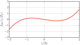
Figure 1: External perturbation $f_{DC}(z)=z^{3}/3-z\langle z^{2}\rangle$ exciting the dipole compression (DC) mode. The value of $\langle z^{2}\rangle$ was calculated using a Maxwell–Boltzmann distribution with thermal radius $Z_{T}=\sqrt{2k_{B}T/(m\omega_{z}^{2})}$.

According to linear response theory Pitaevskii2016 the time evolution of the expectation value $\delta\langle F\rangle(t)=\int dz\delta n(z,t)f_{DC}(z)$ follows the law Zambelli2001

$$\delta\langle F\rangle(t)=\frac{\lambda\hbar}{k_{B}T}\int_{-\infty}^{+\infty}d\omega^{\prime}S_{F}(\omega^{\prime})\left[1-\cos(\omega^{\prime}t)\right]\ ,$$ (26)

where $S_{F}(\omega)$ is the dynamic structure factor relative to the excitation operator $F$, see Eq. (8). In the hydrodynamic regime a single frequency, provided by Eq. (6), will appear in the time evolution of the signal. According to the results of Table 2, this frequency will evolve continuously from the low temperature T value $\sqrt{6}\omega_{z}$ (weakly interacting limit) or $3\omega_{z}$ (Tonks-Girardeau limit) to the large T value $\sqrt{7}\omega_{z}$. In Fig. 2(a) we show the time dependence of the signal $\delta\langle F\rangle(t)$ predicted in the high $T$ hydrodynamic limit. If instead the system is in the collisionless regime of high temperature, and hence $S_{F}(\omega)=\sigma[\delta(\omega-\omega_{z})+\delta(\omega-3\omega_{z})+\omega\to-\omega]$ (we have set $\sigma_{1}=\sigma_{3}\equiv\sigma$, according to the discussions presented at the end of the previous Sec. III), the signal will exhibit a typical beating involving the two frequencies, as reported in 2(b).

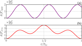
Figure 2: Time evolution of the expectation value $\delta\langle F\rangle$, in units of oscillator time $T_{ho}=2\pi/\omega_{z}$, following the perturbation of the dipole compression mode (see text).
In the hydrodynamic regime of high temperatures (a) the signal is characterized by the single frequency $\sqrt{7}\omega_{z}$, while in the collisionless regime of high T (b) by a periodic beating of the 2 frequencies $\omega_{z}$ and $3\omega_{z}$.

The observation of the transition between a single frequency signal to the beating regime can then be considered a signature of the transition between the hydrodynamic to the collisionless regime. A transition of similar nature was observed in the study of the scissors mode of 3D Bose gases in a deformed harmonic potential where the frequency has a single value at low temperature in the superfluid Bose-Einstein condensed phase, while the spectrum exhibits a beating between two frequencies for temperatures larger than the critical temperature where the system is in the non superfluid collisionless regime GueryOdelin1999 ; Marago2000 .

V Conclusions

In this paper we have calculated the collective frequencies of a 1D harmonically trapped Bose gas in different regimes of interaction, temperature and number of particles.

We have developed two different theoretical methods: the hydrodynamic approach, rewritten in an easier variational formulation, and the more microscopic sum-rule approach. While the first method can be applied only within the Local Density Approximation (LDA) and enables us to calculate the hydrodynamic frequencies for all interaction and temperature regimes, the sum-rule approach allows us to calculate the collective frequencies even beyond the LDA and in the collisionless regime of high temperatures.

The inverse energy weighted ($m_{-1}$), the energy weighted ($m_{1}$) and the cubic energy weighted ($m_{3}$) sum rules are calculated and their applicability to exploit the behaviour of the collective frequencies at zero as well as at finite temperature have been explicitly discussed. We have furthermore developed the formalism of the virial theorem which permits to derive more compact expressions for the average excitation frequencies, defined through the ratio $\hbar^{2}\omega^{2}=m_{3}/m_{1}$.

The combined use of the hydrodynamic and sum rule approaches enables us to draw important conclusions about the temperature dependence of the collective frequencies. While in the case of the lowest breathing mode the frequencies in the high temperature hydrodynamic and collisionless regimes coincide and are equal to $2\omega_{z}$, where $\omega_{z}$ is the oscillator frequency, a different scenario emerges in the case of the dipole compression mode excited by the operator $f_{DC}(z)=z^{3}/3-z\langle z^{2}\rangle$. In the dipole compression case, the hydrodynamic approach in fact predicts the value $\sqrt{7}\omega_{z}$ for the collective frequency, while in the collisionless regime the same operator gives rise to the excitation of two different frequencies given by $\omega_{z}$ and $3\omega_{z}$. By calculating the response of the system to a sudden perturbation of the form $\lambda f_{DC}(z)\Theta(t)$, we predict a typical beating between the two frequencies whose experimental observation would provide a useful signature of the achievement of the collisionless regime. The investigation of the temperature dependence of the dipole compression mode is then expected to provide valuable information on the transition between the hydrodynamic and collisionless regime and on the role of collisions in 1D interacting Bose gases.

The sum rule approach is also expected to provide a useful tool to explore the behaviour of the dipole compression frequencies when the Local Density Approximation is not available at zero as well as at finite temperature and for different interaction regimes. This will be the object of a future investigation.