POINCARÉ, SCALE AND CONFORMAL SYMMETRIES: GAUGE PERSPECTIVE AND COSMOLOGICAL RAMIFICATIONS

THÈSE

SOUMISE À LA FACULTÉ DES SCIENCES DE BASE

LABORATOIRE DE PHYSIQUE DES PARTICULES ET DE COSMOLOGIE

PROGRAMME DOCTORAL EN PHYSIQUE

ÉCOLE POLYTECHNIQUE FÉDÉRALE DE LAUSANNE

POUR L’OBTENTION DU GRADE DE DOCTEUR ÈS SCIENCES

PAR

Georgios Konstantinou Karananas

Adviser: Prof. Mikhail Shaposhnikov

Suisse, juillet 2016

© Georgios Karananas, 2016

Abstract

Symmetries are omnipresent and play a fundamental role in the description of Nature. Thanks to them, we have at our disposal nontrivial selection rules that dictate how a theory should be constructed. This thesis, which is naturally divided into two parts, is devoted to the broad physical implications that spacetime symmetries can have on the systems that posses them.

In the first part, we focus on local symmetries. We review in detail the techniques of a self-consistent framework – the coset construction – that we employed in order to discuss the dynamics of the theories of interest. The merit of this approach lies in that we can make the (spacetime) symmetry group act internally and thus, be effectively separated from coordinate transformations. We investigate under which conditions it is not needed to introduce extra compensating fields to make relativistic as well as nonrelativistic theories invariant under local spacetime symmetries and more precisely under scale (Weyl) transformations. In addition, we clarify the role that the field strength associated with shifts (torsion) plays in this context. We also highlight the difference between the frequently mixed concepts of Weyl and conformal invariance and we demonstrate that not all conformal theories (in flat or curved spacetime), can be coupled to gravity in a Weyl invariant way. Once this “minimalistic” treatment for gauging symmetries is left aside, new possibilities appear. Namely, if we consider the Poincaré group, the presence of the compensating modes leads to nontrivial particle dynamics. We investigate in detail their behavior and we derive constraints such that the theory is free from pathologies.

In the second part of the thesis, we make clear that even when not gauged, the presence of spontaneously broken (global) scale invariance can be quite appealing. First of all, it makes possible for the various dimensionful parameters that appear in a theory to be generated dynamically and be sourced by the vacuum expectation value of the Goldstone boson of the nonlinearly realized symmetry – the dilaton. If the Standard Model of particle physics is embedded into a scale-invariant framework, a number of interesting implications for cosmology arise. As it turns out, the early inflationary stage of our Universe and its present-day acceleration become linked, a connection that might give us some insight into the dark energy dynamics. Moreover, we show that in the context of gravitational theories which are invariant under restricted coordinate transformations, the dilaton instead of being introduced ad hoc, can emerge from the gravitational part of a theory. Finally, we discuss the consequences of the nontrivial way this field emerges in the action.

Keywords: Poincaré invariance, scale invariance, conformal invariance, gauge theory, gravity, cosmology.

Résumé

Les symétries sont omniprésentes et jouent un rôle fondamental dans la description de la nature. Grâce à elles, nous avons à notre disposition des règles de sélection non triviales qui dictent la construction des théories physiques.

Cette thèse, qui est naturellement divisé en deux parties, est consacrée aux vastes implications physiques que les symétries d’espace-temps peuvent avoir sur les systèmes qui les possèdent. Dans la première partie, nous nous concentrons sur les symétries locales. Nous examinons en détail les techniques d’un cadre auto-cohérent – coset construction – que nous avons employé pour examiner les théories qui nous intéressent. Le mérite de cette approche réside dans le fait que nous pouvons faire agir le groupe de symétrie en interne et donc, être efficacement séparé des transformations de coordonnées. Nous étudions les conditions dans lesquelles il n’est pas nécessaire d’introduire des champs de compensation supplémentaires pour rendre une théorie relativiste ou non-relativiste invariante par rappord aux symétries d’espace-temps locales et plus précisément par les transformations de changement d’échelle (transformation de Weyl). En outre, nous clarifions le rôle que le tenseur du champ associé aux déplacements (torsion) joue dans ce contexte. Nous soulignons également la différence entre les concepts souvent mixtes de transformation de Weyl et d’invariance conforme et nous démontrons que toutes les théories conformes (en espace-temps plat ou courbé), ne peuvent pas être couples à la gravité d’une manière invariante sous transformation de Weyl. Si ce traitement “ minimaliste ” pour jauger les symétries est laissé de côte, de nouvelles possibilités apparaissent. Si nous considérons le groupe de Poincaré, la présence des modes de compensation conduit à une dynamique des particules non triviale. Nous étudions en détail leur comportement et nous en déduisons des contraintes pour que la théorie soit exempte de pathologies.

Dans la deuxième partie de la thèse, nous montrons clairement que même lorsque l’invariance globale en changements d’échelle n’est pas jaugé, une brisure spontanée de cette symétrie peut être très attrayante. Tout d’abord, il est possible de générer dynamiquement les différents paramètres dimensionels qui apparaissent dans la théorie. Ceux-ci proviennent ensuite de la valeur moyenne dans le vide du boson de Goldstone de la symétrie brisée - le dilaton. Si le modèle standard de la physique des particules est intégré dans un cadre invariant par les changements d’échelle, un certain nombre d’ implications intéressantes pour la cosmologie se posent. Il se trouve, que la phase d’inflation de notre Univers et son accélération actuelle deviennent liée, une connexion qui pourrait nous donner un aperçu de la dynamique de l’énergie sombre. Enfin, nous montrons que dans le cadre des théories de la gravitation invariantes sous les transformations de coordonnées restreintes, le dilaton peut sortir du secteur gravitationnel d’une théorie au lieu d’être introduit ad hoc. Nous discutons les conséquences intéressantes de la façon dont ce champ émerge dans l’action.

Mots clés: invariance de Poincaré , invariance en changements d’échelle, invariance conforme, théorie de jauge, gravitation, cosmologie.

Chapter 1   Introduction

The Standard Model (SM) of particle physics that describes the electroweak and strong interactions has enabled us to explain in a self-consistent manner a plethora of phenomena. Especially after the discovery of the Higgs boson, SM could be thought of as a predictive effective field theory valid up to energies comparable to the gravitational scale $M_{P}=2.435\times 10^{18}$ GeV.

Despite its unprecedented success, we now understand that the SM is not a complete theory for a number of reasons. From the experimental point of view, it is not possible to address in its context several well established observational facts, like for example the neutrino masses and oscillations, the baryon asymmetry of the Universe and the origin of dark matter. From the theoretical point of view, the SM suffers – among others – from two severe fine-tuning problems, namely the hierarchy and cosmological constant problems. For the former, according to the rules of the effective field theory, the Higgs mass receives large radiative corrections, making it very sensitive to whatever physics lie beyond the SM. Therefore, its smallness requires an extreme fine-tuning in order to compensate for these contributions that are related to the ultraviolet dynamics. For the latter, its predicted value is approximately $M_{P}^{4}$, which is by many orders of magnitude larger than the one observed.

Although these problems do not pose a threat to the consistency of theory, there is no (satisfactory) explanation on what could be the underlying principle making the electroweak scale and the cosmological constant so small as compared to $M_{P}$.

One of the directions towards a possible resolution of the aforementioned theoretical puzzles is to allow certain parameters to be small provided that the symmetry of the theory is enhanced when these are set to zero. If this line of reasoning is applied to the SM, one observes that responsible for the smallness of the Higgs mass and the cosmological constant term could be the presence of exact scale and/or conformal invariance.

In general, theories exhibiting scale and conformal invariance (see, for example, [1, 2]) constitute a very interesting and rich subject for investigations. They appear ubiquitously for describing physical systems, whenever a separation of scales exists. The presence of these symmetries restricts sufficiently the dynamics, so that many properties of the system can be inferred and in some cases, the theory can even be solved completely. Thus, they give an important handle on quantum field theory (for recent progress see [3, 4, 5, 6, 7]).

In particular, if the SM is considered as part of a larger scale or conformally invariant framework, the resulting theory should ultimately be confronted with observations. For it to be phenomenologically viable – apart from incorporating gravity in a consistent with all the symmetries manner – the additional symmetry that it enjoys should be spontaneously broken; this leads to the appearance of a Goldstone boson, the dilaton. As a result, all the scales (at the classical level) can have a common origin: the vacuum expectation value of the dilaton.

It is well known that all classical considerations concerning scale and conformal theories might not survive at the quantum level. This is almost a trivial statement, since a mass scale that explicitly breaks the classical symmetry is introduced when a theory is regularized. However, if this mass scale is related to the vacuum expectation value of the dilaton, then the symmetries of the system remain anomaly-free when quantum corrections are taken into account [8, 9, 10, 11]. Notice though that if such a regularization prescription is used, the loop expansion will generate an infinite number of divergences, therefore an infinite number of counter-terms (not necessarily with the same functional form as the terms in the tree-level theory) will be needed in order to account for them. As we already mentioned, gravity should be part of any realistic model and so, the requirement of renormalizability has to be abandoned in any case. Notice though, that this should not be considered as a drawback, as long as we end up with a predictive effective field theory.

Our purpose in this thesis is to investigate several formal (part I) as well as phenomenological (part II) aspects associated with theories that possess spacetime symmetries. More specifically, in part I, we address Poincaré, scale and conformal invariance from a gauge perspective and we discuss in great detail the role of the compensating fields that have to be introduced. Part II, deals with the cosmological ramifications of scale invariance and with various properties of the dilaton field. For the convenience of the reader, each part contains its own outline.

Part I Theoretical considerations

Chapter 2   Outline of Part I

This part of the thesis is exclusively devoted to formal aspects of gauged spacetime symmetries. In chapter 3, we show that a natural way to get a handle on the dynamics and implications of the systems under consideration is provided by the coset construction. This technique is extremely powerful and very useful, for it allows to systematically build invariant (effective) actions using only symmetry arguments. When dealing with spacetime symmetries, this method makes it possible to completely disentangle the gauge (internal) transformations from the coordinate ones, in complete analogy with the situation in Yang-Mills theories [12].

One illustrative example for realizing the potential of the coset construction, is to consider the gauging of the Poincaré group and consequently the emergence of the gravitational interaction. Conventionally, gravity is treated in the context of Einstein’s theory of General Relativity (GR). However, one can follow the paradigm of the SM and take the gauge approach as a guiding principle.

Even though this approach to gauging is certainly not unique, it is more practical than the conventional one, see for example [13, 14, 15, 16]; the gauge field associated with translations (vielbein) is automatically guaranteed to have an inverse, and more importantly, both field strengths – curvature $\omega$ and torsion $T$ – transform covariantly under the group operations. Therefore, the Lagrangian describing the dynamics of the theory can be straightforwardly written down by considering all possible invariants constructed from curvature and torsion at a given order in derivatives

$$\mathscr{L}=\mathscr{L}_{0}+\mathscr{L}_{1}(\omega,T)+\mathscr{L}_{2}(\omega,T)+\ldots\$$ (2.1)

where $\mathscr{L}_{0},\mathscr{L}_{1},\ldots,$ contain terms with zero derivatives (cosmological constant), one derivative (scalar curvature, Holst term) etc.

The theory in which both curvature and torsion are present, is known in the literature as Poincaré Gravitational Theory (PGT). One might wonder if the presence of the degrees of freedom associated with the connection is a desirable feature. We will be back to this point in a while. It should be noted that if the goal is to eliminate the extra modes and recover the Einstein-Hilbert action from the PGT, then the connection should be expressed in terms of derivatives of the vielbein by imposing the covariant constraint of vanishing torsion. This fact should not come as a surprise, since it can well be the case that the number of fields needed to gauge a spacetime symmetry is smaller than what would be expected. The investigation of when this is actually possible has to be carried out in a systematic way, especially when conformal theories are considered. Let us explain why this is the case. A very powerful tool for studying these systems is coupling them to a nondynamical metric [3, 5, 11]. In an even more general setup, all the couplings are considered as background sources [18]. It is usually assumed that a conformally invariant theory can be embedded in a curved background in a Weyl invariant manner. It is necessary that a theory be conformal in flat spacetime, in order to couple it to gravity in a Weyl-invariant way. It has been shown that the condition becomes sufficient, only if actions with at most one derivative of conformally variant fields are considered [19] (see also [20]). However, to the best of our knowledge, there is no proof for the condition to be sufficient in general.

The authors of the interesting work [19] proceed as follows. Given a scale-invariant theory in flat spacetime, it can be made Weyl invariant by gauging dilatations with the help of an additional field $W_{\mu}$ (Weyl gauging). It so happens that the Weyl variation of a certain combination of the gauge field 

$$\Theta_{\mu\nu}=\nabla_{\mu}W_{\nu}-W_{\mu}W_{\nu}+\frac{1}{2}g_{\mu\nu}W^{\sigma}W_{\sigma}\ ,$$ (2.2)

where $\nabla$ denotes the standard covariant derivative and $g_{\mu\nu}$ the metric, does not depend on $W_{\mu}$. It is proportional to the variation of the Schouten tensor

$$S_{\mu\nu}=R_{\mu\nu}-\frac{R}{2(n-1)}g_{\mu\nu}\ ,$$ (2.3)

with the following convention for the curvatures

$$R=R^{\mu}_{\mu},\leavevmode\nobreak\ \leavevmode\nobreak\ R_{\mu\nu}=R^{\leavevmode\nobreak\ \leavevmode\nobreak\ \leavevmode\nobreak\ \sigma}_{\sigma\mu\leavevmode\nobreak\ \nu}\leavevmode\nobreak\ \leavevmode\nobreak\ \text{and}\leavevmode\nobreak\ \leavevmode\nobreak\ R^{\leavevmode\nobreak\ \leavevmode\nobreak\ \leavevmode\nobreak\ \sigma}_{\lambda\mu\leavevmode\nobreak\ \nu}=\partial_{\lambda}\Gamma_{\mu\nu}^{\sigma}-\partial_{\mu}\Gamma_{\lambda\nu}^{\sigma}+\Gamma_{\lambda\rho}^{\sigma}\Gamma_{\mu\nu}^{\rho}-\Gamma_{\mu\rho}^{\sigma}\Gamma_{\lambda\nu}^{\rho}\ .$$ (2.4)

Therefore, if the gauge field enters the Lagrangian only in the combination (2.2), it is possible to trade it for the expression in (2.3), leaving all the symmetries intact. As a result, the theory becomes Weyl invariant and no additional degrees of freedom are introduced. The authors call this procedure Ricci gauging. Lastly, they prove that for a theory without higher derivatives of conformally variant fields, the described Weyl gauging leads necessarily to the appearance of the tensor (2.2), provided the theory is conformal. Consequently, these theories can be made Weyl invariant when coupled to gravity.

The tensor composed of the Weyl gauge field and possessing the transformation properties of (2.2) can be found by trial and error, but a systematic recipe can be easily provided by the coset construction, as we show in chapter 4. When this formalism is applied to the Poincaré group plus dilatations, the aforementioned relation between $\Theta_{\mu\nu}$ and $S_{\mu\nu}$ follows immediately from the requirement (or better say the covariant constraint) of vanishing torsion. Meanwhile, if one does not insist on having a torsionless theory, then $W_{\mu}$ can be shown to be related to one of the irreducible pieces of the torsion tensor, something that was realized many years ago in [21].

There is a number of questions that arise at this point. To start with, it is natural to wonder whether Ricci gauging can be applied to higher-derivative conformal theories as well. It turns out that its range of applicability is quite vast, even though there are certain subtleties that arise due to the presence of more than one derivatives. Actually, if we consider for example a quartic in derivatives theory of a scalar field in an arbitrary number of spacetime dimensions $n>2$, it is a straightforward (although a bit algebraically involved) exercise to couple it to gravity in a Weyl invariant manner using this procedure.

What is interesting is that certain terms in the Lagrangian of the resulting theory, blow up at the limit $n\to 2$. In chapter 5, we demonstrate that is an indication that the Weyl invariant generalization of a conformal higher-derivative theory does not exist in two spacetime dimensions. Actually, this “obstruction” does not appear only in $n=2$, but is present in all (even) dimensions, if the number of derivatives acting on a field exceeds $n$. This implies that it is not always possible for a conformally invariant theory to be made Weyl invariant. Even though the two notions of Weyl and conformal symmetry are used interchangeably, it should be stressed that the former is not just the curved-space generalization of the latter, but rather a different concept. To put in other words, for a theory invariant under diffeomorphisms $\times$ Weyl, its flat limit automatically produces a theory which is conformal; the opposite is not always true.

Yet another point worth investigating is whether nonrelativistic theories can also be coupled to a curved background in a Weyl invariant way using only the geometrical data. Notice that there has been renewed interest in these theories in the context of many body systems/condensed matter physics, which has been partially sparked by [22, 23]. As we illustrate in chapter 6, the role of torsion here is indispensable, since for the concept of Weyl invariance to even exist, these theories must necessarily be torsionful. Moreover, it is always possible to express the spatial part of the Weyl gauge field in terms of degrees of freedom already present in the theory. As for the temporal part, whether or not it can be eliminated depends on the (nonrelativistic) symmetry group under consideration. For the Lifshitz algebra plus dilatations, there is no obstacle to its elimination, therefore the situation is similar to what occurs with Lorentz-invariant theories. On the other hand, for a theory invariant under the centrally extended Galilei algebra plus dilatations this is not the case, because the presence of boosts complicates considerably the situation. However, even in this case, as long as the temporal part of the gauge field is absent, such a theory is going to be automatically Weyl-symmetric.

Up until this point, we have been exclusively interested on how to achieve invariance of a theory under a symmetry group by keeping the minimal number of compensating gauge fields. However, new and quite interesting possibilities appear if the extra degrees of freedom are not eliminated. Coming back to the PGT, certain torsionful theories [24, 25, 26], have attracted considerable attention, since they are free from pathologies and have very interesting cosmological phenomenology. In general, not all theories in which torsion is propagating are ghost and tachyon free. In chapter 7, we have carried out a detailed analysis of the spectrum of the most general theory that results from the gauging of the Poincaré group and contains terms at most quadratic in the field strengths. We have allowed for parity-odd terms in the action and we have derived the conditions for absence of ghosts and tachyons.

Chapter 3   Gauging spacetime symmetries

The necessary ingredients for building an effective field theory are the field/particle content and symmetries. The latter impose constraints on a Lagrangian, for it (or better to say the action) should be a singlet under the symmetry transformations. Once all the symmetries of a system are known, the number of free parameters in the Lagrangian is reduced.

The reason why it may be needed to go from rigid symmetries to gauged ones is twofold. On the one hand, the background gauge fields act like sources for the corresponding conserved currents. Gauge invariance in this case puts severe constraints (selection rules) on the partition function: integrating out dynamical fields leads – in the absence of anomalies – to a gauge-invariant partition function. On the other hand, the gauge field theories are an appropriate language to talk about massless vector and tensor degrees of freedom, e.g. photons and gravitons.

Any global symmetry group can be made local by introducing a sufficient number of corresponding compensators (gauge fields) with appropriate transformation properties. A question that naturally arises is whether this number can be smaller than the number of generators of the symmetry group considered. For internal symmetries (the ones that commute with the generators of spacetime translations), this does not seem to be the case. However, for spacetime symmetries the gauging may not require as many fields as there are generators. For example, as we will demonstrate later, the Poincaré group can be made local without introducing the spin connection as an independent field, but rather as a function of the vielbein (at least for torsionless theories). We will also show that some Weyl invariant theories do not require the introduction of a gauge field to account for the local scale transformations, since its role can be played by a certain combination of curvature tensors or torsion.

The action of spacetime symmetries on the fields, obtained as an induced representation, is related to the nonlinear realization of symmetries. Therefore, when talking about certain physical systems we find that the coset construction provides the appropriate language. It allows one to circumvent certain difficulties related to the transformation properties of the fields under the corresponding symmetry group, automatically providing the necessary building blocks. In this introductory chapter, based mainly on [27, 28, 17], we review in detail the basic ingredients of this approach and discuss its relevance for gauging spacetime symmetries.

3.1 Internal symmetries

The nonlinear realization of internal symmetries (the ones that commute with the generators of spacetime translations) in flat spacetime was introduced in [29, 30] and it is used to obtain the building blocks for a theory that exhibits a specific symmetry breaking pattern $S\to S_{0}$. In other words, it allows one to construct the most general action of a group $S$ such that when restricted to its subgroup $S_{0}$, it becomes a linear representation.

The procedure can be described as follows. For the symmetry breaking pattern, one realizes the action of the group $S$ on the coset space $S/S_{0}$ by left multiplication. Choosing the coset representative as

$$\Omega=e^{i\pi T}\in S\ ,$$ (3.1)

where $T$ is the set of all broken generators and $\pi$ (Goldstone fields) constitutes a parametrization of the coset, one gets the transformation

$$s\Omega=\Omega^{\prime}\bar{s}_{0}\ ,\leavevmode\nobreak\ \leavevmode\nobreak\ \leavevmode\nobreak\ \text{with}\leavevmode\nobreak\ \leavevmode\nobreak\ \leavevmode\nobreak\ \bar{s}_{0}\equiv\bar{s}_{0}(\pi,s)\in S_{0}\ .$$ (3.2)

Central role to this approach plays the Maurer-Cartan form

$$\Omega^{-1}\partial_{\mu}\Omega\ ,$$ (3.3)

that is calculated using the commutation relations of the group under consideration. If we denote by $t$ all the unbroken generators, this expression can be written as

$$\Omega^{-1}\partial_{\mu}\Omega=i\nabla_{\mu}\pi\,T+i\omega_{\mu}t\ ,$$ (3.4)

and it is easy to check that under (3.2), it transforms as

$$\left(\Omega^{-1}\partial_{\mu}\Omega\right)^{\prime}=\bar{s}_{0}\left(\Omega^{-1}\partial_{\mu}\Omega\right)\bar{s}_{0}^{-1}+\bar{s}_{0}\partial_{\mu}\bar{s}_{0}^{-1}\ .$$ (3.5)

For compact groups, the above translates into the corresponding transformations of $\nabla_{\mu}\pi$ and $\omega_{\mu}$

$$\nabla_{\mu}\pi^{\prime}T =\bar{s}_{0}\,\nabla_{\mu}\pi^{\prime}T\,\bar{s}_{0}^{-1}\ ,$$ (3.6)

$$i\omega_{\mu}^{\prime}t =\bar{s}_{0}\,i\omega_{\mu}t\,\bar{s}_{0}^{-1}+\bar{s}_{0}\partial_{\mu}\bar{s}_{0}^{-1}\ ,$$

which can be used to write automatically $S$-invariant Lagrangians by constructing singlets of the subgroup $S_{0}$.

The gauging of the group $S$ within this framework goes along the standard lines; it is achieved by promoting the partial derivative $\partial_{\mu}$ in (3.3) to a covariant derivative $\tilde{D}_{\mu}$ including gauge fields that correspond to each generator of the symmetry group and under the action of $S$ transform as

$$\tilde{A}^{\prime}_{\mu}=s\tilde{A}_{\mu}s^{-1}+s\partial_{\mu}s^{-1}\ .$$ (3.7)

3.2 Spacetime symmetries

The difference between internal and spacetime symmetries is that the latter are usually (if not necessarily) realized on the infinite dimensional spaces of fields. These infinite dimensional representations are induced representations that are defined in the following way. For a group $K$, its subgroup $K_{0}\subset K$ that is realized on a linear space $V$, there is a natural action of the group $K$ on the coset $K/K_{0}$ by left multiplications. For example, let us take $K$ to be the $n$-dimensional Poincaré group and $K_{0}$ to be the Lorentz group. It is clear that in this case $K/K_{0}=\mathbb{R}^{n}$. The action of $K$ on the coset is as follows 

$$ke^{iPy}=e^{iP(\Lambda y+a)}\bar{k}_{0}(k)\ ,$$ (3.8)

where $k\in K$, $\bar{k}_{0}(k)\in K_{0}$, $P_{A}$ are momenta, $\Lambda^{A}_{\ B}$ correspond to Lorentz rotations, $y_{A}$ are Cartesian coordinates on the coset $\mathbb{R}^{n}$ and $a_{A}$ are parameters of the translations. Considering a representation of the Lorentz group

$$\rho:K_{0} \to {GL}(V)\ ,$$ (3.9)

$$T_{\bar{k}_{0}}\Psi = \rho(\bar{k}_{0})\Psi\ ,$$

we define the induced representation of the full Poincaré group according to

$$\left(T_{k}\Psi\right)(y^{\prime})=\rho(\bar{k}_{0}(k))\Psi(y)\ ,$$ (3.10)

which corresponds to the standard transformation of a field

$$\Psi_{(\Lambda,a)}(y)=D(\Lambda)\Psi(\Lambda^{-1}y-a)\ .$$ (3.11)

Even though the generators $P_{A}$, which correspond to the coset $K/K_{0}$, are not broken and are realized linearly on the space of fields, the very construction of this representation makes it natural to include the momenta in the coset (3.1) when discussing the breaking and/or gauging of spacetime symmetries. Consequently, for the symmetry group $G$ (with algebra $\mathfrak{g}$) that includes both internal and spacetime symmetries and that is broken down to a subgroup $H$ (with algebra $\mathfrak{h}$), one gets the coset in the form

$$\Omega=e^{iPx}e^{i\pi(x)T}\ ,$$ (3.12)

where by $T$ we denote all the broken generators (not only the internal ones). The way to introduce a different set of coordinates on the spacetime manifold is to have them appearing in the coset representative through the auxiliary functions $y^{A}(x)$, which means that in general we may write

$$\Omega=e^{iPy(x)}e^{i\pi(x)T}\ .$$ (3.13)

Under the action of the spacetime symmetry group $K$, the coordinates transform according to

$$ke^{iPy(x)}=e^{i{Py(x^{\prime})}}\bar{k}_{0}\ ,\leavevmode\nobreak\ \leavevmode\nobreak\ \leavevmode\nobreak\ \text{with}\leavevmode\nobreak\ \leavevmode\nobreak\ \leavevmode\nobreak\ \bar{k}_{0}\equiv\bar{k}_{0}(x,k)\ .$$ (3.14)

These transformations may be viewed in a different way, namely, keeping the coordinates $x$ unchanged while transforming the functions $y^{A}(x)\to y^{{}^{\prime}A}(x)$

$$ke^{iPy(x)}=e^{iPy^{\prime}(x)}\bar{k}_{0}\ .$$ (3.15)

The reason for this choice becomes clear when the gauging of a spacetime symmetry group is considered, for in this case one does not have to take into account the transformation of the fields due to the change of coordinates $x$ and the gauging goes along the lines of that for internal symmetries. However, by doing so, the additional functions $y^{A}(x)$, with very specific transformation properties, had to be introduced. Of course, they are not physical and should be dispensed with. This is easily achieved by simply demanding that the resulting theory is invariant under diffeomorphisms as well.

In a sense, introducing these additional spurious fields allows us to decouple the diffeomorphisms from the (local) transformations under the spacetime symmetry group. The gauge fields $\tilde{A}_{\mu}$ transform in the standard way (3.7) under the local spacetime transformations and separately under the diffeomorphisms $x\to x^{\prime}$,

$$\tilde{A}^{\prime}_{\mu}(x^{\prime})=\tilde{A}_{\nu}(x)\frac{\partial x^{\nu}}{\partial x^{{}^{\prime}\mu}}\ .$$ (3.16)

The Maurer-Cartan form can now be written as

$$\Omega^{-1}\tilde{D}_{\mu}\Omega=ie_{\mu}^{A}P_{A}+i\nabla_{\mu}\pi\,T+i\omega_{\mu}t\ ,$$ (3.17)

where as before $P_{A}$ are momenta, whereas $t$ and $T$ are the rest of the unbroken and broken generators respectively. For symmetry groups with the following schematic structure of commutation relations

$$\left[t,t\right] =t\ ,$$ (3.18)

$$\left[t,P\right] =P\ ,$$

$$\left[t,T\right] =T\ ,$$

and upon using the definition of the transformation of the coset representative

$$g\Omega=\Omega^{\prime}\bar{h}(y,g)\ ,$$ (3.19)

we find that the transformations of $\nabla_{\mu}\pi$, $\omega_{\mu}$ and $e_{\mu}^{A}$, are given by

$$\nabla_{\mu}\pi^{\prime}T =\bar{h}\,\nabla_{\mu}\pi^{\prime}T\,\bar{h}^{-1}(\pi,s)\ ,$$ (3.20)

$$i\omega_{\mu}^{\prime}t =\bar{h}\,i\omega_{\mu}t\,\bar{h}^{-1}+\bar{h}\partial_{\mu}\bar{h}^{-1}\ ,$$

$$e^{{}^{\prime}A}_{\mu}P_{A} =e^{A}_{\mu}\,\bar{h}(\pi,g)P_{A}\bar{h}^{-1}(\pi,g)\ ,$$

The coefficients $e_{\mu}^{A}$ due to their specific transformation properties under the diffeomorphisms (3.16) can be thought of as the vielbein.

As a result, we have the necessary tools to analyze a system with spontaneously broken symmetries. For example, any $H$-invariant function of $\nabla_{\mu}\pi$ would produce a Lagrangian which is “secretly” $G$ invariant, if one also uses $e_{\mu}^{\nu}$ to build an invariant measure. Similarly, the connection can be used to construct higher derivative terms and/or coupling to matter fields.

It should be noted that the main feature of the nonlinear realization of spacetime symmetries – as compared to internal ones – is the counting of degrees of freedom. For the case of internal symmetries, the number of Goldstone modes is always equal to the number of broken generators. For spacetime symmetries, this is not always true, since it is not rare that a smaller number of Goldstone bosons is enough to realize a symmetry breaking pattern. This happens because the fluctuations produced by the action of all broken generators on the vacuum are not independent. From the physical point of view, this phenomenon manifests itself through the equations of motion, when at low energies certain modes may become gapped and, therefore, can be explicitly integrated out. From a more formal perspective, it can be understood with the help of the inverse Higgs mechanism, which consists of imposing covariant (consistent with all symmetries) constraints on the system and solving them algebraically, thus, reducing the number of necessary fields [31, 32, 33, 34]. Notice, however, that the constraints that can be solved are those for which the commutator of a broken generator $T$ with the momentum contains another broken generator $T^{\prime}$

$$\left[P,T\right]\supset T^{\prime}\ .$$ (3.21)

In this case, the Goldstone corresponding to $T$ is expressed in terms of the derivatives of other fields, by solving $\nabla_{\mu}\pi_{T^{\prime}}=0$.

3.2.1 Coset construction and the Poincaré group

The Poincaré group is the semi-direct product of translations $P_{A}$ and Lorentz transformations $J_{AB}$ and its algebra is defined by the following commutation relations between the generators

$$\left[P_{A},P_{B}\right] =0\ ,$$ (3.22)

$$\left[J_{AB},P_{C}\right] =i\left(\eta_{BC}P_{A}-\eta_{AC}P_{B}\right)\ ,$$

$$\left[J_{AB},J_{CD}\right] =i\left(J_{AD}\eta_{BC}+J_{BC}\eta_{AD}-J_{BD}\eta_{AC}-J_{AC}\eta_{BD}\right)\ .$$

The role of this group in particle physics is fundamental and twofold. On one hand, it dictates the symmetries of the underlying Minkowski spacetime of Special Relativity. On the other hand, particle states in quantum field theories are classified according to the unitary irreducible representations of this particular group [35, 36].

The pursuit of a gravitational theory with better microscopic behaviour that GR, as well as the fact that Yang-Mills theories enjoyed big success, initiated investigations [13, 14] that eventually lead to the formulation of a gravitational theory that results from the gauging of the Poincaré group [15, 16]. As we have already mentioned, within the framework of the coset construction, gravity is obtained by promoting the 10 (constant) parameters of the group to depend arbitrarily on position, and at the same time to demand that the theory be invariant under general coordinate transformations (diffeomorphisms) [37, 38, 17]. Since we want Lorentz rotations to be unbroken, then according to the discussion in the previous chapter, the coset representative contains only the momenta [17]

$$\Omega=e^{iP_{A}y^{A}}\ .$$ (3.23)

Using the standard formulas for two operators $X$ and $Y$

$$e^{-Y}Xe^{Y} = X+\left[X,Y\right]+\frac{1}{2}\left[\left[X,Y\right],Y\right]+\dots\ ,$$ (3.24)

$$e^{-Y}\partial_{\mu}e^{Y} = \partial_{\mu}Y+\frac{1}{2}\left[\partial_{\mu}Y,Y\right]+\frac{1}{6}\left[\left[\partial_{\mu}Y,Y\right],Y\right]+\dots\ ,$$ (3.25)

we find that the Maurer-Cartan form (3.17) becomes

$$\Omega^{-1}\left(\partial_{\mu}+i\tilde{e}^{A}_{\mu}P_{A}+\frac{i}{2}\tilde{\omega}^{AB}_{\mu}J_{AB}\right)\Omega=ie_{\mu}^{A}P_{A}+\frac{i}{2}\omega^{AB}_{\mu}J_{AB}\ .$$ (3.26)

Here $\tilde{e}_{\mu}^{A}$ , $\tilde{\omega}_{\mu}^{AB}$ are the 40 a priori independent gauge fields corresponding to translations and Lorentz rotations respectively, while their counterparts without the tilde are defined as

$$e_{\mu}^{A}=\tilde{e}_{\mu}^{A}+\partial_{\mu}y^{A}-\tilde{\omega}_{\mu}^{AB}y_{B}\ ,\leavevmode\nobreak\ \leavevmode\nobreak\ \leavevmode\nobreak\ \leavevmode\nobreak\ \leavevmode\nobreak\ \omega_{\mu}^{AB}=\tilde{\omega}_{\mu}^{AB}\ .$$ (3.27)

It is straightforward to check that the transformation of $e_{\mu}^{A}$ under the action of the local Lorentz group is

$$e_{\mu}^{A}\rightarrow\Lambda^{A}_{\ B}e_{\mu}^{B}\ ,$$ (3.28)

whereas under a diffeomorphism $x\rightarrow x^{\prime}$,

$$e_{\mu}^{A}(x)\rightarrow e_{\mu}^{A}(x)\frac{\partial x^{\nu}}{\partial x^{{}^{\prime}\mu}}\ .$$ (3.29)

Consequently, $e_{\mu}^{A}$ can be interpreted as a vielbein that is used to mix spacetime and Lorentz indices, to define the metric $g_{\mu\nu}=e_{\mu}^{A}e_{\nu}^{B}\eta_{AB}$, and to construct the diffeomorphism-invariant measure

$$d^{n}x\,\det e_{\mu}^{A}\equiv d^{n}x\,\det e\ .$$ (3.30)

Notice that if we do not require that the theory be invariant under the full group of diffeomorphisms, then the construction of the invariant measure is not necessary. For example one may be interested in theories invariant only with respect to transverse diffeomorphisms (TDiff), see for example [39, 40, 41] and references therein. In this case, the theory is invariant only under the subgroup of coordinate transformations with Jacobian equal to unity, thus we can allow for the presence of arbitrary powers of the vielbein (or equivalently the metric) determinant. We will discuss in more detail these theories in the last chapter of the thesis.

The field $\omega^{AB}_{\mu}$, in turn, under a Lorentz transformation behaves as

$$\omega^{AB}_{\mu}\rightarrow\omega^{CD}_{\mu}\Lambda_{C}^{\leavevmode\nobreak\ A}\Lambda_{D}^{\leavevmode\nobreak\ B}+\left(\Lambda\partial_{\mu}\Lambda^{-1}\right)^{AB}\ ,$$ (3.31)

thus it can be interpreted as the spin connection.

The covariant derivative, as in any gauge theory, is defined by

$$D_{A}=E^{\mu}_{A}\left(\partial_{\mu}+\frac{i}{2}\omega^{AB}_{\mu}J_{AB}\right)\ ,$$ (3.32)

where we denoted with $E^{\mu}_{A}$ the inverse vielbein, and at this stage, $\omega_{\mu}^{AB}$ are considered as independent degrees of freedom. To express them in terms of the vielbein, as it is usually done for torsionless gravity, we should impose some constraints. We will be back to this point shortly.

As customary, the field strength tensors, torsion $T$ and curvature $\omega$, are readily obtained by considering the commutator of two covariant derivatives acting for example on a vector field. They are respectively given by

$$T_{\mu\nu}^{A}=\partial_{\mu}e_{\nu}^{A}-\partial_{\nu}e_{\mu}^{A}-\omega_{\mu B}^{A}e_{\nu}^{B}+\omega_{\nu B}^{A}e_{\mu}^{B}\ ,$$ (3.33)

$$\omega_{\mu\nu}^{AB}=\partial_{\mu}\omega_{\nu}^{AB}-\partial_{\nu}\omega_{\mu}^{AB}-\omega_{\mu}^{AC}\omega_{\nu C}^{B}+\omega_{\nu}^{AC}\omega_{\mu C}^{B}\ ,$$ (3.34)

and it can be checked that they transform covariantly, as they should.

Even though vielbein and connection are independent degrees of freedom, it should be made clear that this need not necessarily be the case. As we argued before, localizing a spacetime symmetry may not require the introduction of as many (gauge) fields as there are generators. For the case at hand, the commutators of $P_{A}$ and $J_{AB}$ (see (3.22)), suggest that the covariant constraints

$$T_{\mu\nu}^{A}=0\ ,$$ (3.35)

could be solved. We end up with the well-known

$$\omega^{AB}_{\mu}=\bar{\omega}^{AB}_{\mu} =-\frac{1}{2}\left[E^{\nu A}\left(\partial_{\mu}e_{\nu}^{B}-\partial_{\nu}e_{\mu}^{B}\right)-E^{\nu B}\left(\partial_{\mu}e_{\nu}^{A}-\partial_{\nu}e_{\mu}^{A}\right)\right.$$ (3.36)

$$\left.-e_{\mu C}E^{\nu A}E^{\lambda B}\left(\partial_{\nu}e_{\lambda}^{C}-\partial_{\lambda}e_{\nu}^{C}\right)\right]\ ,$$

clearly exhibiting that for torsionless theories, the Poincaré group can be made local without the connection being an independent field.

Chapter 4   Weyl and Ricci gauging from the coset construction

In this chapter, following closely [28], we show that Weyl and Ricci gauging can be carried out in a more systematic way, by employing the coset construction. We illustrate that the relation between the structure $\Theta_{\mu\nu}$ composed of the Weyl vector and the Schouten tensor $S_{\mu\nu}$ given in (2.2) and (2.3) respectively, can be obtained by the analog of the inverse Higgs constraints (3.21). We use the word analog, because as we have already mentioned what is usually called inverse Higgs mechanism is a constraint that can be solved algebraically with respect to a certain field (or fields). In our case (for a theory without torsion) we find a constraint that leads to the relation

$$(n-2)\Theta_{\mu\nu}\simeq S_{\mu\nu}\ .$$ (4.1)

The reason we use the symbol “$\simeq$”, is because we want to stress that the above expression is not an equality in the sense that the field $W_{\mu}$ can be expressed in terms of the metric; it is clear that this equation cannot be solved algebraically. Rather, what we imply is that the combination on the left-hand side of (4.1) transforms identically to the one on the right-hand side. Therefore, it can be substituted by the latter in a consistent with all the symmetries way. We also show that once the requirement of having a torsionless theory is relaxed, $W_{\mu}$ is found to be equal to one of the irreducible components of the torsion tensor.

It should also be noted that contrary to the standard gauging of internal symmetries, the Weyl gauge field $W_{\mu}$ appears in the covariant derivative not only with the operator of dilatations, but with the generators of Lorentz transformations as well. This happens because scale invariance is a spacetime symmetry (which does not commute with spacetime translations). In our treatment, the form of the covariant derivative follows automatically.

This chapter is organized as follows. In Sec. 4.1, we gauge scale transformations and obtain the relation between $\Theta_{\mu\nu}$ and $S_{\mu\nu}$ . In Sec. 4.2, we demonstrate how Ricci gauging works by considering two examples. The first one is the purely gravitational Weyl square theory in four dimensions, and the second one is the $n$-dimensional generalization of the Riegert theory. In Sec. 4.3, we discuss how Weyl gauging can take place if torsion is present in the theory. Sec. 4.4, contains the conclusions.

4.1 Local scale transformations

In the previous chapter we showed how the gravitational interaction emerges in the context of the coset construction by gauging the Poincaré group. Our goal here is to obtain a Weyl-invariant theory, consequently, we will gauge scale transformations as well. In this case, the coset representative is identical to the one in (3.23) and does not contain generators other than the momenta.

For the Maurer-Cartan form we obtain

$$\Omega^{-1}\left(\partial_{\mu}+i\tilde{e}^{A}_{\mu}P_{A}+\frac{i}{2}\tilde{\omega}^{AB}_{\mu}J_{AB}+i\tilde{W}_{\mu}D\right)\Omega=ie_{\mu}^{A}P_{A}+\frac{i}{2}\omega^{AB}_{\mu}J_{AB}+iW_{\mu}D\ ,$$ (4.2)

where, as before, we denoted with $\tilde{e}_{\mu}^{A}$ and $\tilde{\omega}_{\mu}^{AB}$ the gauge fields for translations and Lorentz transformations, and in addition we introduced the fields $\tilde{W}_{\mu}$ which are associated with dilatations. Notice that in the presence of the new symmetry, the relation between the quantities without and with tilde are

$$e_{\mu}^{A}=\tilde{e}_{\mu}^{A}+\partial_{\mu}y^{A}-\tilde{\omega}_{\mu}^{AB}y_{B}+\tilde{W}_{\mu}y^{A}\ ,\leavevmode\nobreak\ \leavevmode\nobreak\ \leavevmode\nobreak\ \leavevmode\nobreak\ \leavevmode\nobreak\ \omega_{\mu}^{AB}=\tilde{\omega}_{\mu}^{AB}\ ,\leavevmode\nobreak\ \leavevmode\nobreak\ \leavevmode\nobreak\ \leavevmode\nobreak\ \leavevmode\nobreak\ W_{\mu}=\tilde{W}_{\mu}\ .$$ (4.3)

Using the analog of (3.19)

$$\Omega^{\prime}=g\Omega\bar{h}^{-1}(y,g),\leavevmode\nobreak\ \leavevmode\nobreak\ \text{with}\leavevmode\nobreak\ \leavevmode\nobreak\ \bar{h}=e^{-it\alpha(y,g)}\in H=SO(n-1,1)\times\mathbb{R}\ ,$$ (4.4)

and the commutation relations presented in Appendix B, one finds the transformation properties of the gauge fields

	$e^{{}^{\prime}A}_{\mu}$	$\omega^{{}^{\prime}AB}_{\mu}$	$W^{\prime}_{\mu}$
$J$	$e_{\mu}^{B}\Lambda_{B}^{\leavevmode\nobreak\ A}$	$\omega^{CD}_{\mu}\Lambda_{C}^{\leavevmode\nobreak\ A}\Lambda_{D}^{\leavevmode\nobreak\ B}+\left(\Lambda\partial_{\mu}\Lambda^{-1}\right)^{AB}$	$W_{\mu}$
$D$	$e^{-\alpha}e_{\mu}^{A}$	$\omega^{AB}_{\mu}$	$W_{\mu}+\partial_{\mu}\alpha$

The transformations of $e_{\mu}^{A}$, $\omega_{\mu}^{AB}$ and $W_{\mu}$ are precisely the ones for the vielbein, spin connection and the Weyl gauge field. According to the rules of the coset construction, the covariant derivative of a matter field $\psi$ is now given by

$$D_{A}\psi=E^{\mu}_{A}\left(\partial_{\mu}+\frac{i}{2}\omega^{AB}_{\mu}J_{AB}+iW_{\mu}D\right)\psi\ .$$ (4.5)

It is clear that by analogy with the previous chapter, one can construct generalized field strength tensors corresponding to shifts, Lorentz and also scale transformations

$$\centering e_{\mu\nu}^{A}\@add@centering =\partial_{\mu}e_{\nu}^{A}-\partial_{\nu}e_{\mu}^{A}-\omega_{\mu B}^{A}e_{\nu}^{B}+\omega_{\nu B}^{A}e_{\mu}^{B}+W_{\mu}e_{\nu}^{A}-W_{\nu}e_{\mu}^{A}\ ,$$ (4.6)

$$\omega^{AB}_{\mu\nu} =\partial_{\mu}\omega_{\nu}^{AB}-\partial_{\nu}\omega_{\mu}^{AB}-\omega_{\mu C}^{A}\omega_{\nu}^{CB}+\omega_{\nu C}^{A}\omega_{\mu}^{CB}\ ,$$ (4.7)

$$W_{\mu\nu} =\partial_{\mu}W_{\nu}-\partial_{\nu}W_{\mu}\ ,$$ (4.8)

that transform covariantly

	$e^{{}^{\prime}A}_{\mu\nu}$	$\omega^{{}^{\prime}AB}_{\mu\nu}$	$W^{\prime}_{\mu\nu}$
$J$	$e_{\mu\nu}^{B}\Lambda_{B}^{\leavevmode\nobreak\ A}$	$\omega^{CD}_{\mu\nu}\Lambda_{C}^{\leavevmode\nobreak\ A}\Lambda_{D}^{\leavevmode\nobreak\ B}$	$W_{\mu\nu}$
$D$	$e^{-\alpha}e_{\mu\nu}^{A}$	$\omega^{AB}_{\mu\nu}$	$W_{\mu\nu}$

Inspection of the commutation relations given in Appendix B, reveals that once we set

$$e_{\mu\nu}^{A}=0\ ,$$ (4.9)

we obtain

$$\omega^{AB}_{\mu}=\bar{\omega}^{AB}_{\mu}+\delta\omega^{AB}_{\mu}\ ,$$ (4.10)

where $\bar{\omega}^{AB}_{\mu}$ is the standard spin connection for a torsionless theory presented in (3.36), and

$$\delta\omega_{\mu}^{AB}=I_{\mu\nu}^{AB}W^{\nu}\ ,\ \ \ I_{\mu\nu}^{AB}=e_{\nu}^{A}e_{\mu}^{B}-e_{\nu}^{B}e_{\mu}^{A}\ .$$ (4.11)

Plugging the expression for $\omega$ to the definition of the covariant derivative (4.5), we find that it can rewritten as follows

$$D_{A}\psi=E^{\mu}_{A}\left(\partial_{\mu}+\frac{i}{2}\bar{\omega}^{AB}_{\mu}J_{AB}-ie^{A}_{\mu}e^{B}_{\nu}W^{\nu}J_{AB}+iW_{\mu}D\right)\psi\ .$$ (4.12)

In particular, for a vector field $V^{A}$ with scaling dimension $\Delta_{V}$, we get

$$e^{B}_{\mu}D_{B}V^{A}=\partial_{\mu}V^{A}-\bar{\omega}^{A}_{\mu B}V^{B}+(e_{\mu}^{A}E_{B}^{\nu}-E^{\nu A}e_{\mu B})V^{B}W_{\nu}-\Delta_{V}W_{\mu}V^{A}\ .$$ (4.13)

We can clearly see now the reason why the Weyl gauge field “couples” to spin as well. Using the Christoffel symbols defined in Appendix A, one can show that the expression for the covariant derivative (4.12) coincides with the one used in [19].

Notice that the field strength tensor corresponding to shifts is not the only covariant structure. Even though imposing another constraint is not in the spirit of the standard inverse Higgs mechanism, it can be done consistently. The gauge field $\omega_{\mu}^{AB}$ depends on $W_{\mu}$; therefore, we may hope to relate certain structure depending on this vector to a tensor that depends only on the vielbein.

Plugging the expression (4.10) to the formula (4.7), we get

$$\omega^{AB}_{\mu\nu}=\bar{\omega}^{AB}_{\mu\nu}+\delta\omega^{AB}_{\mu\nu},$$ (4.14)

with $\bar{\omega}_{\mu\nu}^{AB}$ given by (7.8) and repeated here for the convenience of the reader

$$\bar{\omega}_{\mu\nu}^{AB}=\partial_{\mu}\bar{\omega}_{\nu}^{AB}-\partial_{\nu}\bar{\omega}_{\mu}^{AB}-\bar{\omega}_{\mu C}^{A}\bar{\omega}_{\nu}^{CB}+\bar{\omega}_{\nu C}^{A}\bar{\omega}_{\mu}^{CB}\ ,$$ (4.15)

and

$$\delta\omega^{AB}_{\mu\nu} =I^{AB}_{\nu\lambda}\nabla_{\mu}W^{\lambda}-I^{AB}_{\mu\lambda}\nabla_{\nu}W^{\lambda}+\left(e^{A}_{\mu}e^{B}_{\nu}-e^{B}_{\mu}e^{A}_{\nu}\right)W^{2}$$ (4.16)

$$+\left(e^{A}_{\nu}W^{B}-e^{B}_{\nu}W^{A}\right)W_{\mu}-\left(e^{A}_{\mu}W^{B}-e^{B}_{\mu}W^{A}\right)W_{\nu}\ ,$$

where we used the vielbein to manipulate the indices of $W_{\mu}$, so that $W^{2}=W_{B}W^{B}=W_{\mu}W^{\mu}$.

None of the constraints imposed on $\omega^{AB}_{\mu\nu}$, although consistent with its transformation properties, can be solved algebraically with respect to $W_{\mu}$. Nevertheless, imposing

$$\omega_{\mu\nu}+\omega_{\nu\mu}\simeq 0\ ,\ \ \ \text{with}\ \ \ \omega_{\mu\nu}\equiv\omega^{AB}_{\mu\sigma}E^{\sigma}_{B}e_{\nu A}\ ,$$ (4.17)

and using (4.14) leads to (4.1), which coincides with the expression obtained in [19], except that we use a different convention for the Riemann curvature tensor, see (2.4).

The substitution $S_{\mu\nu}$ for $\Theta_{\mu\nu}$ is similar in spirit to the standard inverse Higgs phenomenon, according to which, certain degrees of freedom are not needed to realize a symmetry breaking pattern and as a result, they can be eliminated. Note, however, that the opposite substitution is not legitimate (at least not for arbitrary field configurations), since the Schouten tensor is subject to the Bianchi identity

$$\nabla^{\mu}S_{\mu\nu}-\nabla_{\nu}S=0\ ,$$ (4.18)

which is not satisfied by $\Theta_{\mu\nu}$.

In [19], it was shown that the substitution (4.1) can always be made for conformal (in flat spacetime) theories with at most one derivative of conformally variant fields. In this case, the invariance under Weyl rescalings does not require the introduction of extra degrees of freedom, since the inhomogeneous pieces of the transformation that appear in the derivatives can be compensated for by curvature terms.

It should also be noted that the constraint (4.17) taken as an equality, only implies the equivalence between the Schouten tensor $S_{\mu\nu}$ and the symmetric part of $\Theta_{\mu\nu}$. However, in a weaker sense (that is, equivalence of the transformation properties), it is possible to relate $S_{\mu\nu}$ to the full $\Theta_{\mu\nu}$. In fact, the antisymmetric part is given by

$$2\Theta_{\mu\nu}^{\text{anti}}=\partial_{\mu}W_{\nu}-\partial_{\nu}W_{\mu}=W_{\mu\nu}\ ,$$ (4.19)

which is invariant under Weyl transformations and can be safely added to $\Theta_{\mu\nu}^{\text{sym}}$, resulting in (4.1).

4.2 Examples

4.2.1 Weyl tensor

As a first example, we build the Weyl-invariant action for pure gravity in a four dimensional spacetime, without coupling to matter. After imposing the constraint $e^{A}_{\mu\nu}=0$, we are left with three objects: two Weyl-invariant curvatures $\omega^{AB}_{\mu\nu}$ and $W_{\mu\nu}$, and the Weyl covariant vielbein $e^{A}_{\mu}$. In order to account for the noninvariance of the measure $d^{4}x\,\det e$, it should be multiplied four times by the inverted vielbein

$$\int d^{4}x\,\det e\,E^{\mu}_{A}\,E^{\nu}_{B}\,E^{\lambda}_{C}\,E^{\sigma}_{D}\ .$$ (4.20)

The lowest-order (in derivatives) diffeomorphism-invariant action, which also respects the gauged scale and Poincaré symmetries can be obtained by all possible contractions of (4.20) with

$$W_{\mu\nu}W_{\lambda\sigma}\leavevmode\nobreak\ \leavevmode\nobreak\ \leavevmode\nobreak\ \text{and}\leavevmode\nobreak\ \leavevmode\nobreak\ \leavevmode\nobreak\ \omega^{AB}_{\mu\nu}\omega^{AB}_{\lambda\sigma}\ .$$ (4.21)

The first term leads to the following obviously Weyl-invariant action (we do not assume parity invariance)

$$S_{1}=\int d^{4}x\,\det e\,\left(c_{1}W_{\mu\nu}W^{\mu\nu}+c_{2}\epsilon^{\mu\nu\lambda\sigma}W_{\mu\nu}W_{\lambda\sigma}\right),$$ (4.22)

with $c_{1}$ and $c_{2}$ being constants and $\epsilon^{\mu\nu\lambda\sigma}=E^{\mu}_{A}\,E^{\nu}_{B}\,E^{\lambda}_{C}\,E^{\sigma}_{D}\epsilon^{ABCD}$. The contractions with $\omega^{AB}_{\mu\nu}\omega^{AB}_{\lambda\sigma}$ can be simplified once the constraint (4.17) is imposed. The antisymmetric part of $\omega_{\mu\nu}$ from (4.17) is proportional to $\partial_{\mu}W_{\nu}-\partial_{\nu}W_{\mu}$, which already has been taken into account in (4.22). We may thus consider only configurations with $\omega^{AB}_{\mu\nu}E^{\nu}_{B}=0$. As a result, the only possible contractions are the following

$$\epsilon^{IJKL}E^{\mu}_{I}E^{\nu}_{J}E^{\rho}_{K}E^{\sigma}_{L}\epsilon_{ABCD}\leavevmode\nobreak\ \omega_{\mu\nu}^{AB}\omega_{\rho\sigma}^{CD}\ ,$$ (4.23)

and

$$\epsilon^{IJKL}E^{\mu}_{I}E^{\nu}_{J}E^{\rho}_{K}E^{\sigma}_{L}\leavevmode\nobreak\ \eta_{AC}\eta_{BD}\omega_{\mu\nu}^{AB}\omega_{\rho\sigma}^{CD}\ ,\ \ \ \epsilon^{IJKL}E^{\mu}_{I}E^{\nu}_{J}E^{\rho}_{A}E^{\sigma}_{B}\leavevmode\nobreak\ \eta_{KC}\eta_{LD}\omega_{\mu\nu}^{AB}\omega_{\rho\sigma}^{CD}\ .$$ (4.24)

Simplifying these expressions, leads to

$$S_{2}=\int d^{4}x\,\det e\,\left(c_{3}C_{\mu\nu\lambda\sigma}C^{\mu\nu\lambda\sigma}+c_{4}\epsilon^{\kappa\rho\lambda\sigma}C_{\mu\nu\kappa\rho}C^{\mu\nu}_{\leavevmode\nobreak\ \leavevmode\nobreak\ \leavevmode\nobreak\ \lambda\sigma}\right),$$ (4.25)

where $c_{3}$, $c_{4}$ are constants, and $C_{\mu\nu\lambda\sigma}$ is the Weyl tensor

$$C_{\mu\nu\lambda\sigma} =R_{\mu\nu\lambda\sigma}+\frac{1}{n-2}\left(g_{\nu\lambda}R_{\mu\sigma}+g_{\mu\sigma}R_{\nu\lambda}-g_{\nu\sigma}R_{\mu\lambda}-g_{\mu\lambda}R_{\nu\sigma}\right)$$ (4.26)

$$+\frac{1}{(n-1)(n-2)}\left(g_{\mu\lambda}g_{\nu\sigma}-g_{\mu\sigma}g_{\nu\lambda}\right)R\ .$$

4.2.2 Higher derivative action

Here, we wish to get a better grasp on the range of applicability of Ricci gauging. To be more precise, we want to understand whether or not the presence of more than one derivative of a conformally variant field constitutes an obstruction in the Ricci gauging. To achieve that, we consider a theory with a higher number of derivatives of a scalar field, namely, a conformally invariant theory in an $n$-dimensional flat spacetime given by the following action

$$S_{\Box^{2}}=\int d^{n}x(\Box\phi)^{2}\ .$$ (4.27)

According to the coset construction described previously, we introduce the covariant derivative (4.12) for the field $\phi$ in the following way

$$D_{A}\phi=E^{\mu}_{A}\left(\nabla_{\mu}\phi-\Delta_{\phi}W_{\mu}\phi\right)\ ,$$ (4.28)

where $\Delta_{\phi}=\frac{n}{2}-2$ is the scaling (mass) dimension of $\phi$. Therefore,

$$e^{B}_{\mu}D_{B}D_{A}\phi =\partial_{\mu}D_{A}\phi-\bar{\omega}_{\mu A}^{\leavevmode\nobreak\ \leavevmode\nobreak\ B}D_{B}\phi+(e_{\mu A}E^{\nu B}-E^{\nu}_{A}e_{\mu}^{B})D_{B}\phi W_{\nu}$$ (4.29)

$$-(\Delta_{\phi}+1)W_{\mu}D_{A}\phi\ ,$$

where we used the fact that the scaling dimension of $D_{A}\phi$ is equal to $\Delta_{\phi}+1$. As a result, the following substitution

$$\Box\phi\to D_{A}D^{A}\phi=\nabla^{2}\phi+2W_{\mu}\nabla^{\mu}\phi-\left(\frac{n}{2}-2\right)\left(\nabla_{\mu}W^{\mu}+\frac{n}{2}W^{\mu}W_{\mu}\right)\ ,$$ (4.30)

where $\nabla^{2}=g^{\mu\nu}\nabla_{\mu}\nabla_{\nu}$, leads to the Weyl-invariant action

$$S_{\Box^{2}}=\int d^{n}x\,\det e(D_{A}D^{A}\phi)^{2}\ .$$ (4.31)

The question we would like to address now is whether it is possible to use Ricci gauging [or, equivalently, the weak form of the constraint (4.1)] to completely get rid of the field $W_{\mu}$. Lengthy but straightforward calculations lead to

$$S_{\Box^{2}} =\int d^{n}x\det e\leavevmode\nobreak\ \left\{\vphantom{\frac{A}{B}}(\nabla^{2}\phi)^{2}-\left[4\Theta_{\mu\nu}-(n-2)\Theta g_{\mu\nu}\right]\nabla^{\mu}\phi\nabla^{\nu}\phi\right.$$ (4.32)

$$\left.-\phi^{2}\left[\frac{n-4}{2}\nabla^{2}\Theta+(n-4)\Theta_{\mu\nu}\Theta^{\mu\nu}-\frac{n(n-4)}{4}\Theta^{2}\right]\right.$$

$$\left.-\phi^{2}(n-4)W^{\nu}\nabla^{\mu}\left(\Theta_{\mu\nu}-g_{\mu\nu}\Theta\right)\vphantom{\frac{A}{B}}\right\}\ ,$$

where $\Theta=\Theta^{\mu}_{\mu}$. Notice that the dependence of the action on $W_{\mu}$ for $n=4$ is only through the tensor $\Theta_{\mu\nu}$ and Ricci gauging can be used without any trouble. Although, for general $n$, there is an explicit $W_{\mu}$ dependence in the last term, it is clear that after the substitution (we assume $n\neq 2$)

$$\Theta_{\mu\nu}\to\frac{1}{n-2}S_{\mu\nu}\ ,$$ (4.33)

this term drops out by virtue of the Bianchi identity (4.18). Therefore, it is shown that the theory given by the Lagrangian (4.31) can be Ricci gauged in an arbitrary (not equal to two) number of dimensions. The resulting action can be written in the following form

$$S_{\Box^{2}}=\int d^{n}x\sqrt{g}\phi\mathcal{Q}_{4}(g)\phi,$$ (4.34)

with

$$\mathcal{Q}_{4}(g) =\nabla^{2}+\nabla^{\mu}\left[\left(\frac{4}{n-2}S_{\mu\nu}-g_{\mu\nu}S\right)\nabla^{\nu}\right]-\frac{n-4}{2(n-2)}\nabla^{2}S$$ (4.35)

$$-\frac{n-4}{(n-2)^{2}}S_{\mu\nu}S^{\mu\nu}+\frac{n(n-4)}{4(n-2)^{2}}S^{2}\ ,$$

being the Paneitz operator [42], which is the Weyl covariant generalization of $\Box^{2}$, see also Appendix D.

At this point, it is natural to wonder what happens when $n\to 2$. In this limit, the coefficients in front of the Schouten tensor (2.3) diverge. At the same time, the Schouten tensor itself vanishes due to the following relation between Ricci curvatures in two dimensions

$$R_{\mu\nu}=\frac{R}{2}g_{\mu\nu}\ .$$ (4.36)

Therefore, this is a case that has to be examined separately. Actually, as we will prove in the next chapter, it is not possible to construct a fourth-order Weyl covariant operator in $n=2$ spacetime dimensions. Based on this observation, we will be able to show that even though the notions of Weyl and conformal invariance are used interchangeably, the former is not just the curved-space generalization of the latter, but rather a different concept.

4.3 Torsionful theory

The field strength corresponding to shifts $e^{A}_{\mu\nu}$ and the generalized spin connection $\omega^{AB}_{\mu}$ have the same symmetry properties; therefore, they have equal number of independent components. This is the reason why we were able to solve the inverse Higgs constraint (4.9) with respect to the $\omega^{AB}_{\mu}$ and express it in terms of the vielbein and the Weyl vector field $W_{\mu}$. This way, we built a Weyl-invariant torsionless theory. Here we look for an alternative solution to this constraint.

In order to understand what the possible solutions might be, we should analyze the structure of irreducible representations of $e^{A}_{\mu\nu}$, since they can be set to zero independently. Any tensor that possesses the symmetries of the quantity $e^{A}_{\mu\nu}$, admits the following decomposition in an $n$-dimensional spacetime (see also Appendix C). A vector,

$$\varepsilon_{\mu}=E^{\nu}_{A}e^{A}_{\mu\nu}\ ,$$ (4.37)

a completely antisymmetric tensor

$$\mathscr{A}^{\sigma_{1}\dots\sigma_{n-3}}=\frac{1}{n}\,\epsilon^{\sigma_{1}\sigma_{2}\cdots\sigma_{n-3}\mu\nu\lambda}e_{\lambda A}\,e_{\mu\nu}^{A}\ ,$$ (4.38)

and a traceless tensor with mixed symmetries

$$\mathscr{E}_{\mu\nu}^{A}=e_{\mu\nu}^{A}-\frac{3}{2(n-1)}\left(\varepsilon_{\mu}e_{\nu}^{A}-\varepsilon_{\nu}e^{A}_{\mu}\right)-\frac{1}{2}E^{\lambda A}\left(e^{B}_{\lambda\mu}e_{\nu B}-e^{B}_{\lambda\nu}e_{\mu B}\right)\ .$$ (4.39)

Written in this form, the constraints (4.9), make it clear that (4.38) and (4.39) can only be solved with respect to their counterparts contained in $\omega^{AB}_{\mu}$. However, for the vector part (4.37) there are two options. The first one, which has been chosen in the previous section, is to eliminate the vectorial part of the spin connection. The second one is to solve the constraint with respect to $W_{\mu}$, keeping $\omega^{AB}_{\mu}E^{\mu}_{B}$ undetermined, which yields a torsionful theory.

We see from (4.6) that

$$W_{\mu}e_{\nu}^{A}-W_{\nu}e_{\mu}^{A}=-T_{\mu\nu}^{A}\ ,$$ (4.40)

where the torsion tensor $T_{\mu\nu}^{A}$ was defined in (3.33) and reads

$$T_{\mu\nu}^{A}\equiv\partial_{\mu}e_{\nu}^{A}-\partial_{\nu}e_{\mu}^{A}-\omega_{\mu B}^{A}e_{\nu}^{B}+\omega_{\nu B}^{A}e_{\mu}^{B}\ ,$$ (4.41)

Tracing (4.40), we obtain

$$W_{\mu}=-\frac{1}{n-1}\upsilon_{\mu}\ ,$$ (4.42)

where we denoted with $\upsilon_{\mu}$ the torsion vector

$$\upsilon_{\mu}=E^{\nu}_{A}T_{\mu\nu}^{A}=E^{\nu}_{A}\left(\partial_{\mu}e_{\nu}^{A}-\partial_{\nu}e_{\mu}^{A}+\omega_{\nu B}^{A}e_{\mu}^{B}\right)\ .$$ (4.43)

It is straightforward to check that under Weyl rescalings the vector $\upsilon_{\mu}$ transforms exactly as the Weyl field, i.e.

$$\upsilon^{\prime}_{\mu}=\upsilon_{\mu}-(n-1)\partial_{\mu}\alpha\ .$$ (4.44)

As a result, once we consider nonvanishing torsion, the degrees of freedom carried by $W_{\mu}$ can be traded for the vector $\upsilon_{\mu}$.

4.4 Summary and Outlook

In this chapter we touched upon the question of whether the conformal invariance of a system in flat spacetime implies that the system can be coupled to gravity in a Weyl-invariant way. We used the prescription of the standard coset construction in order to gauge scale transformations (along with the Poincaré group), leading to a Weyl-invariant (in curved spacetime) theory. It was demonstrated that the main ingredient needed for Ricci gauging, namely the relation between the additional gauge field corresponding to the local scale transformations and the Ricci curvature – first obtained in [19] – can be extracted from the analog of the inverse Higgs constraint.

This revealed that the two structures (4.1) transform in the same way, and therefore, whenever the tensor $\Theta_{\mu\nu}$ appears in the action, it can be substituted by its counterpart without any contradiction with the underlying symmetries. The answer to the question of whether such a prescription for conformally invariant theories leads to a complete elimination of the gauge field $W_{\mu}$ does not have a definite answer at the moment and can only be divined.

We presented a couple of examples of how Ricci gauging works. First, we obtained the Weyl-invariant action for pure gravity in four spacetime dimensions, which is given, as is well known, by the square of the Weyl tensor. Next, we considered a theory with more than one derivative of a scalar field (4.31). In a four dimensional spacetime, the Ricci gauging can be straightforwardly employed. However, it so happens that the scaling dimension of the field is zero in this case; thus, the field is actually conformally invariant. Notice that there is no contradiction with [19], since the condition of having at most one derivative was only imposed on conformally variant fields.

Considering the system in $n\neq 2$, we showed that Ricci gauging can be applied even for theories with more than one derivative of conformally variant fields. In the example we considered, the procedure turned out to be a little bit subtle. Namely, the Weyl gauged Lagrangian cannot be written as a function depending only on $\Theta_{\mu\nu}$, but rather, it also depends explicitly on $W_{\mu}$. However, this dependence drops out, once Ricci gauging is performed.

Finally, we also presented an alternative way of introducing the Weyl symmetry. We showed, by solving the inverse Higgs constraint, that the role of the gauge field associated with local scale transformations can be played by the vector part of the torsion tensor.

Chapter 5   Weyl vs. Conformal

5.1 Introduction

The purpose of this chapter, based to a large extent on [47], is to clarify the difference between the occasionally mixed notions of conformal and Weyl invariance. The conformal symmetry in a $n$-dimensional (not necessarily flat) space-time is defined as the group of coordinate transformations

$$x^{\prime}=F(x)\ ,$$ (5.1)

which leave the metric $g_{\mu\nu}$ invariant up to a conformal factor

$$g_{\mu\nu}(x)=\Omega(x^{\prime})\,g_{\lambda\sigma}^{\prime}(x^{\prime})\,\frac{\partial F^{\lambda}}{\partial x^{\mu}}\frac{\partial F^{\sigma}}{\partial x^{\nu}}\ .$$ (5.2)

For the infinitesimal form of the transformations

$$x^{\prime\mu}=x^{\mu}+f^{\mu}\ ,$$ (5.3)

the relation (5.2) leads to the conformal Killing equations

$$\nabla_{\mu}f_{\sigma}+\nabla_{\sigma}f_{\mu}=\frac{2}{n}g_{\mu\sigma}\nabla f\ ,$$ (5.4)

where we used the shorthand notation $\nabla f=\nabla_{\mu}f^{\mu}$, and we denoted with $\nabla$ the metric-compatible covariant derivative

$$\nabla_{\mu}f_{\nu}=\partial_{\mu}f_{\nu}-\Gamma^{\lambda}_{\mu\nu}f_{\lambda}\ ,$$ (5.5)

with $\Gamma^{\lambda}_{\mu\nu}$ being the Christoffel symbols.

Here, we focus only on theories with scalars, leaving the investigation of fields with non-zero spin for elsewhere. The infinitesimal transformation of a scalar field with scaling (mass) dimension $\Delta_{\phi}$ under the full conformal group can be written in the following compact form

$$\delta_{c}\phi=-\left(f^{\mu}\nabla_{\mu}\phi+\frac{\Delta_{\phi}}{n}\nabla f\phi\right).$$ (5.6)

A system is called conformally invariant if the variation of its action functional $S[g_{\mu\nu},\phi]$ under the full group of conformal transformations (5.6) is zero, i.e.

$$\delta_{c}S[g_{\mu\nu},\phi]=\int d^{n}x\,\frac{\delta S}{\delta\phi}\,\delta_{c}\phi=0\ .$$ (5.7)

Meanwhile, Weyl rescalings constitute another type of transformations, which are given by the simultaneous pointwise transformations of the metric and fields

$$\hat{g}_{\mu\nu}(x) =e^{2\sigma(x)}g_{\mu\nu}(x)\leavevmode\nobreak\ \leavevmode\nobreak\ \leavevmode\nobreak\ \text{and}\leavevmode\nobreak\ \leavevmode\nobreak\ \leavevmode\nobreak\ \hat{\phi}(x) =e^{-\Delta_{\phi}\sigma}\phi(x)\ ,$$ (5.8)

with $\sigma$ being an arbitrary function. Writing the above expressions in their infinitesimal form as

$$\delta_{\sigma}g_{\mu\nu}=2\sigma g_{\mu\nu}\leavevmode\nobreak\ \leavevmode\nobreak\ \leavevmode\nobreak\ \text{and}\leavevmode\nobreak\ \leavevmode\nobreak\ \leavevmode\nobreak\ \delta_{\sigma}\phi=-\Delta_{\phi}\sigma\phi\ ,$$ (5.9)

leads to the following condition for a theory to be Weyl invariant

$$\delta_{\sigma}S[g_{\mu\nu},\phi]=\int d^{n}x\,\sigma\left(2\,\frac{\delta S}{\delta g_{\mu\nu}}g_{\mu\nu}-\Delta_{\phi}\,\frac{\delta S}{\delta\phi}\phi\right)=0\ .$$ (5.10)

Note that (5.6) can be written as

$$\delta_{c}\phi=\delta_{d}\phi+\delta_{\bar{\sigma}}\phi\ ,$$ (5.11)

where we denoted by $\delta_{\bar{\sigma}}\phi$ the Weyl transformation corresponding to the specific value of $\sigma=\bar{\sigma}\equiv\nabla f/n$, and $\delta_{d}\phi$ is the standard transformation of the scalar field under the general coordinate transformations

$$\delta_{d}\phi=-f^{\mu}\partial_{\mu}\phi\ .$$ (5.12)

As a result, equation (5.7) can be rewritten as

$$0=\int d^{n}x\,\frac{\nabla f}{n}\left(2\,\frac{\delta S}{\delta g_{\mu\nu}}g_{\mu\nu}-\Delta_{\phi}\,\frac{\delta S}{\delta\phi}\phi\right)\ ,$$ (5.13)

where we used the fact that the $\delta_{d}\phi$ transformations can be compensated for by the corresponding transformations of the metric (provided the theory is diffeomorphism invariant). It is clear that Weyl invariance implies conformal invariance, but not the other way around, since $\nabla f$ is not an arbitrary function of coordinates.

5.2 Examples

Let us present another way to understand why Weyl invariance necessarily implies conformal invariance in flat space-time. The corresponding conformal Killing equations now read

$$\partial_{\mu}\varepsilon_{\nu}+\partial_{\nu}\varepsilon_{\mu}=\frac{2}{n}\eta_{\mu\nu}\partial_{\lambda}\varepsilon^{\lambda}\ ,$$ (5.14)

with $\eta_{\mu\nu}=\text{diag}\left(1,-1,\ldots\right)$, the Minkowski metric, and $\varepsilon^{\mu}$ being the flat space-time analog of $f^{\mu}$. This set of equations has the following $(n+1)(n+2)/2$ parametric solution for $n\neq 2$

$$\varepsilon^{\mu}=a^{\mu}+\omega^{\mu}_{\leavevmode\nobreak\ \nu}x^{\nu}+cx^{\mu}+2(b\cdot x)x^{\mu}-x^{2}b^{\mu}\ .$$ (5.15)

Here $a^{\mu}$, $\omega_{\mu\nu}=-\omega_{\nu\mu}$, $c$ and $b^{\mu}$ are constants corresponding to translations, Lorentz transformations, dilatations and special conformal transformations (SCT) respectively. In two dimensions, $\varepsilon^{\mu}$ is given by an arbitrary generalized harmonic function.

The standard procedure allows one to build the energy-momentum tensor

$$T^{\text{impr}}_{\mu\nu}=2\frac{\delta S}{\delta g^{\mu\nu}}\Big{|}_{g_{\mu\nu}=\eta_{\mu\nu}}\ ,$$ (5.17)

which is automatically traceless on the equations of motion, see (5.10). As a result, all currents of the form $j_{\mu}=T^{\text{impr}}_{\mu\nu}\varepsilon^{\nu}$, with $\varepsilon^{\mu}$ given in (5.15), are conserved.

Conversely, if a theory is conformally invariant, then according to [48, 49], it is possible to write all currents corresponding to the conformal group in the following way

$$j_{\mu}=T_{\mu\nu}\varepsilon^{\nu}-\partial\varepsilon K_{\mu}+\partial^{\nu}\partial\varepsilon L_{\mu\nu}\ ,$$ (5.18)

where $T_{\mu\nu}$ is the energy-momentum tensor (not necessarily traceless), $K_{\mu}$ is a vector and $L_{\mu\nu}$ is a rank-two tensor such that

$$\partial_{\mu}T_{\mu\nu}=0\ ,\ \ \ T_{\mu\nu}=T_{\nu\mu}\ ,\ \ \ T_{\mu}^{\mu}=n\,\partial_{\mu}K^{\mu}\ \ \ \text{and}\ \ \ K_{\mu}=\partial^{\nu}L_{\nu\mu}\ .$$ (5.19)

Notice that for $n=2$, there is an additional restriction

$$L_{\mu\nu}=\eta_{\mu\nu}L\ ,$$ (5.20)

with $L$ being a scalar function.

The conditions presented above allow to construct the improved (traceless) energy momentum tensor $T^{\text{impr}}_{\mu\nu}$.

However, it is not guaranteed that the theory can be made Weyl invariant. In what follows, we will consider several examples of conformally invariant theories which cannot be made Weyl invariant when coupled to gravity. We should mention though, that we will not consider theories with non-linearly realized space-time symmetries, like in the case of galileons [50]. There, the reason that the conformal invariance of a certain action for the galileon does not imply Weyl invariance, is associated with the fact that this action is actually a Wess-Zumino term, see also [51].

5.2.1 $\Box$

For the purposes of illustration, it is instructive to begin by considering the Lagrangian of a free massless field in a one-dimensional spacetime

$$\mathcal{L}=\frac{\dot{\phi}^{2}}{2}\ .$$ (5.21)

If the scaling dimension of $\phi$ is $\Delta_{\phi}=-1/2$, then the theory is invariant under the one-dimensional conformal group

$$\delta\phi=-\left(\varepsilon\dot{\phi}-\frac{1}{2}\phi\dot{\varepsilon}\right)\ ,$$ (5.22)

where

$$\varepsilon=a+b\,t+\frac{c}{2}\,t^{2}\ ,$$ (5.23)

with $a,b$ and $c$, constants. The conserved currents associated with translations, dilatations and special conformal transformations can be written according to (5.18) as

$$J=\frac{\dot{\phi}^{2}}{2}\varepsilon-\frac{\phi\dot{\phi}}{2}\dot{\varepsilon}+\frac{\phi^{2}}{4}\ddot{\varepsilon}.$$ (5.24)

Clearly, this theory cannot be made Weyl invariant, for there are no geometric structures in $n=1$ one could use to account for the non-invariance of $\dot{\phi}^{2}$.

5.2.2 $\Box^{2}$

Let us now consider the theory given by the following Lagrangian

$$\mathcal{L}_{\Box^{2}}=\frac{1}{2}(\Box\phi)^{2}\ ,$$ (5.25)

with $\Box=\eta^{\mu\nu}\partial_{\mu}\partial_{\nu}$ the D’Alembertian. Using the flat space-time analog of formula (5.6) with $\Delta_{\phi}=n/2-2$, it is straightforward to check that in $n\neq 2$, the variation of this Lagrangian is given by a total derivative

$$\delta\mathcal{L}_{\Box^{2}}=-\partial^{\mu}\left[\varepsilon_{\mu}\mathcal{L}_{\Box^{2}}-\frac{2}{n}\partial^{\nu}\partial\varepsilon\left(\partial_{\mu}\phi\partial_{\nu}\phi-\frac{1}{2}\eta_{\mu\nu}(\partial\phi)^{2}\right)\right]\ .$$ (5.26)

In this case, using the following definitions

$$T_{\mu\nu} =\eta_{\mu\nu}\left(\partial_{\lambda}\phi\partial^{\lambda}\Box\phi+\frac{1}{2}\left(\Box\phi\right)^{2}\right)-\partial_{\mu}\Box\phi\partial_{\nu}\phi-\partial_{\nu}\Box\phi\partial_{\mu}\phi\ ,$$ (5.27)

$$K_{\mu} =\frac{1}{2}\Box\phi\partial_{\mu}\phi+\frac{\Delta_{\phi}}{n}\phi\partial_{\mu}\Box\phi\ ,$$

$$L_{\mu\nu} =\frac{1}{n}\left(2\partial_{\nu}\phi\partial_{\mu}\phi-\eta_{\mu\nu}\left(\partial\phi\right)^{2}+\Delta_{\phi}\eta_{\mu\nu}\phi\Box\phi\right)\ ,$$

it is straightforward to check that the relations presented in (5.19) are satisfied. Therefore, the system is indeed conformally invariant for $n\neq 2$.

As we showed in detail in Sec. 4.2.2, the Weyl-invariant generalization of the theory (5.25), reads 

$$S_{\Box^{2}}=\int d^{n}x\sqrt{g}\phi\,\mathcal{Q}_{4}(g)\,\phi\ ,$$ (5.28)

with $Q_{4}(g)$ the Paneitz operator that was defined in (4.35). As we mentioned in the previous chapter, the above expression is not well defined for $n\to 2$. To understand what is going on in this limit, let us consider the most general ansatz for the operator $Q_{4}(g)$ in two dimensions

$$\mathcal{Q}_{4}(g)=\nabla^{4}+c_{1}\nabla^{\mu}\left(R\nabla_{\mu}\right)+c_{2}\nabla^{2}R+c_{3}R^{2}\ ,$$ (5.29)

with $c_{1},c_{2}$ and $c_{3}$ constants. A straightforward calculation shows the Weyl variation of $\nabla^{4}$ will produce terms that cannot be cancelled by the variation of $R$-dependent terms, for example $\left(\nabla^{\mu}\nabla_{\nu}\sigma\right)\nabla_{\mu}\nabla_{\nu}$. Therefore, for $n=2$ there is no Weyl covariant generalization of the fourth-order differential operator. Hence, in this case, the system (5.25) cannot be coupled to gravity in a Weyl invariant way, although this does not come as a surprise, for as it is clear from (5.27), the condition (5.20) is not satisfied. One can say that the system at hand in a two dimensional space-time, is only invariant under global conformal transformations, which correspond to the six dimensional sub-algebra of the Virasoro algebra. Let us note that global conformal transformations are defined on the two dimensional sphere. The non-zero commutation relations are

$$\left[l_{-1},l_{0}\right]=-l_{-1}\ ,\leavevmode\nobreak\ \leavevmode\nobreak\ \leavevmode\nobreak\ \left[l_{-1},l_{1}\right]=-2l_{0}\ ,\leavevmode\nobreak\ \leavevmode\nobreak\ \leavevmode\nobreak\ \left[l_{0},l_{1}\right]=-l_{1}\ ,$$

$$\left[\bar{l}_{-1},\bar{l}_{0}\right]=-\bar{l}_{-1}\ ,\leavevmode\nobreak\ \leavevmode\nobreak\ \leavevmode\nobreak\ \left[\bar{l}_{-1},\bar{l}_{1}\right]=-2\bar{l}_{0}\ ,\leavevmode\nobreak\ \leavevmode\nobreak\ \leavevmode\nobreak\ \left[\bar{l}_{0},\bar{l}_{1}\right]=-\bar{l}_{1}\ ,$$

where the generators in terms of the complex coordinates $z$ and $\bar{z}$, read

$$l_{-1}=-\partial_{z}\ ,\leavevmode\nobreak\ \leavevmode\nobreak\ \leavevmode\nobreak\ \bar{l}_{-1}=-\partial_{\bar{z}}\,\leavevmode\nobreak\ \leavevmode\nobreak\ \leavevmode\nobreak\ \leavevmode\nobreak\ \text{(translations)}\ ,$$

$$l_{0}=-z\partial_{z}\ ,\leavevmode\nobreak\ \leavevmode\nobreak\ \leavevmode\nobreak\ \bar{l}_{0}=-\bar{z}\partial_{\bar{z}}\,\leavevmode\nobreak\ \leavevmode\nobreak\ \leavevmode\nobreak\ \leavevmode\nobreak\ \leavevmode\nobreak\ \text{(rotations and dilatations)}\ ,$$

$$l_{1}=-z^{2}\partial_{z}\ ,\leavevmode\nobreak\ \leavevmode\nobreak\ \leavevmode\nobreak\ \bar{l}_{1}=-\bar{z}^{2}\partial_{\bar{z}}\leavevmode\nobreak\ \leavevmode\nobreak\ \leavevmode\nobreak\ \text{(SCT)}\ .$$

5.2.3 $\Box^{3}$

The fact that it is impossible to construct a Weyl invariant action for the system (5.25) in two dimensions, is a particular case of a more general result [52, 53, 54], see also [55]. This states that for even number of dimensions, there exist Weyl invariant generalizations of $\Box^{k}$ only for $k\leq\frac{n}{2}$. Therefore, considering a theory with six derivatives in a four dimensional space-time

$$\mathcal{L}_{\Box^{3}}=\frac{1}{2}\left(\partial_{\mu}{\Box}\phi\right)^{2}\ ,$$ (5.30)

one is sure that it cannot be made Weyl invariant. This can be immediately seen by inspecting the Weyl covariant analog of the operator (5.30). It contains terms proportional to

$$\frac{1}{(n-2)(n-4)}B_{\mu\nu}S^{\mu\nu}\ ,\leavevmode\nobreak\ \leavevmode\nobreak\ \leavevmode\nobreak\ \frac{1}{n-4}\nabla^{\mu}\left(B_{\mu\nu}\nabla^{\nu}\right)\ ,$$ (5.31)

thus it does not exist in $n=2$ and $n=4$ dimensions for a non-zero Bach tensor $B_{\mu\nu}$

$$B_{\mu\nu}=C_{\mu\rho\nu\sigma}S^{\rho\sigma}+\nabla^{\rho}\nabla_{\mu}S_{\nu\rho}-\nabla^{2}S_{\mu\nu}\ ,$$ (5.32)

with $C_{\mu\rho\nu\sigma}$ being the Weyl tensor.

However, straightforward computations reveal – taking into account that the scaling dimension of the field in this case is equal to $\Delta_{\phi}=n/2-3$ – that the conformal variation of the Lagrangian (5.30) is also a total derivative

$$\delta\mathcal{L}_{\Box^{3}}=-\partial^{\mu}\left[\varepsilon_{\mu}\mathcal{L}_{\Box^{3}}-\frac{1}{n}\partial^{\nu}\partial\varepsilon\left(4\partial_{\mu}\partial_{\nu}\phi\Box\phi-\frac{1}{2}(\Box\phi)^{2}\left(\frac{n}{2}+3\right)\eta_{\mu\nu}\right)\right]\ .$$ (5.33)

Moreover, one can build the energy-momentum tensor

$$T_{\mu\nu} =\Box^{2}\phi\,\partial_{\mu}\partial_{\nu}\phi-\left(\partial_{\mu}\phi\,\partial_{\nu}\Box^{2}\phi+\partial_{\nu}\phi\,\partial_{\mu}\Box^{2}\phi\right)$$ (5.34)

$$+\partial^{\lambda}\phi\,\partial_{\mu}\partial_{\nu}\partial_{\lambda}\Box\phi+\Box\phi\,\partial_{\mu}\partial_{\nu}\Box\phi+\partial^{\lambda}\Box\phi\,\partial_{\mu}\partial_{\nu}\partial_{\lambda}\phi$$

$$-\partial_{\mu}\Box\phi\,\partial_{\nu}\Box\phi-\eta_{\mu\nu}\left[\frac{1}{2}\left(\partial_{\lambda}\Box\phi\right)^{2}+\partial^{\lambda}\partial^{\sigma}\phi\,\partial_{\lambda}\partial_{\sigma}\Box\phi\right]\ ,$$

as well as the operators

$$K_{\mu} =\alpha\,\partial_{\mu}\partial_{\nu}\phi\,\partial_{\nu}\Box\phi-(n+\alpha)\partial^{\nu}\phi\,\partial_{\mu}\partial_{\nu}\Box\phi-\left(\frac{n}{2}+\alpha\right)\partial_{\mu}\Box\phi\,\Box\phi$$ (5.35)

$$+\left(\alpha+\frac{n}{2}+2\right)\partial_{\mu}\phi\,\Box^{2}\phi+\left(\frac{n}{2}-3\right)\phi\,\partial_{\mu}\Box^{2}\phi\ ,$$

and

$$L_{\mu\nu} = \left(\alpha-\frac{n-10}{4}\right)\partial_{\mu}\phi\,\partial_{\nu}\Box\phi-\left(\alpha+\frac{3n-10}{4}\right)\partial_{\nu}\phi\,\partial_{\mu}\Box\phi$$

$$+ \frac{n-10}{4}\partial_{\mu}\partial_{\nu}\phi\,\Box\phi-\frac{n+10}{4}\phi\,\partial_{\mu}\partial_{\nu}\Box\phi+\frac{3n-2}{4}\eta_{\mu\nu}\phi\,\Box^{2}\phi\ .$$

The above satisfy (5.19) for arbitrary values of the constant $\alpha$, therefore, the theory is conformal in flat space-time. Notice, though, that for $L_{\mu\nu}$ to be symmetric, we have to set $\alpha=-n/4$.

5.2.4 Curved space-time

In order to further expose the difference between the concepts of Weyl and conformal symmetries we consider the curved space-time counterpart of $\Box^{3}$. It is obvious that the sixth-order Weyl covariant operator for $n\neq 2$ and $n\neq 4$ is also conformally invariant for an arbitrary metric. It may happen though that there are no conformal Killings for a specific background to start with. To guarantee that the conformal group is not empty, we stick to Einstein manifolds only, for which

$$R_{\mu\nu}=\frac{R}{n}g_{\mu\nu}\ .$$ (5.36)

It is easy to check that the Bach tensor (5.32) in this case vanishes identically. Therefore, the dangerous terms (5.31) disappear, thus the limit $n\to 4$ of the conformally invariant curved space analog of $\Box^{3}$, can be safely considered. In doing so, one obtains a conformally invariant operator with leading term $\nabla^{6}$.

To illustrate the procedure in more detail, we consider the Paneitz operator, which for Einstein manifolds becomes regular at $n=2$. It is straightforward to check using the relation

$$\nabla_{\mu}\nabla_{\nu}\nabla f+\frac{1}{2n(n-1)}g_{\mu\nu}\left(n\,f^{\sigma}\nabla_{\sigma}R+2\,R\nabla f\right)=0\ ,$$ (5.37)

following from the conformal Killing equations for $n\neq 2$, that the corresponding action

$$S=\int d^{n}x\sqrt{g}\Bigg{[}\nabla^{2}\phi\nabla^{2}\phi -\frac{4-n(n-2)}{2n(n-1)}R\left(\nabla\phi\right)^{2}-\frac{n-4}{4(n-1)}\phi^{2}\nabla^{2}R$$ (5.38)

$$+\frac{(n-2)(n+2)(n-4)}{16n(n-1)^{2}}\phi^{2}R^{2}\Bigg{]}\ ,$$

is invariant under the ($n\neq 2$) conformal transformations, as it should. The limit $n\to 2$ in turn is regular

$$S=\int d^{n}x\sqrt{g}\Bigg{[}\nabla^{2}\phi\nabla^{2}\phi -R\left(\nabla\phi\right)^{2}+\frac{1}{2}\phi^{2}\nabla^{2}R\Bigg{]},$$ (5.39)

and is invariant under global conformal transformations. The reason it is not invariant under the full conformal group is that the relation (5.37) does not follow automatically for two dimensional theories. Rather, it has to be imposed by hand, reducing the conformal group to its subgroup of global transformations. Clearly this is a peculiarity of two dimensions.

5.3 Generalization

The examples we considered clearly show that not any conformally invariant (both in flat and curved space-time) theory can be made Weyl invariant. In fact, there is a whole class of theories not allowing Weyl invariant generalizations. Indeed, as it was mentioned before, according to [52, 53, 54], the Weyl covariant analogs of $\Box^{k}$ exist unless the number of space-time dimensions $n$ is even and less than $k/2$. The impossibility to construct the corresponding operators in even number of dimensions manifests itself through the presence of terms singular at $n=2,4,6,\ldots$ However, it seems plausible that similar to the situation described in the previous section those terms vanish (or at least become regular) once the geometry is restricted to that of Einstein spaces. As a result, the corresponding limit $n\to 4,6,\ldots$ exists and is invariant under conformal transformations (or only global conformal transformations for $n\to 2$).

Since flat spaces are a particular case of Einstein ones, according to the above argument, the theories whose dynamics is described by the Lagrangian in flat space-time

$$\mathcal{L}_{\Box^{k}}=\frac{1}{2}\phi\Box^{k}\phi\$$ (5.40)

are conformal (for $n\neq 2$). We can convince ourselves that this is the case by considering the variation of the Lagrangian with respect to conformal transformations. For $k=2m$ and $k=2m+1$, the Lagrangian can be rewritten as

$$\mathcal{L}_{\Box^{2m}}=\frac{1}{2}(\Box^{m}\phi)^{2}\leavevmode\nobreak\ \leavevmode\nobreak\ \text{and}\leavevmode\nobreak\ \leavevmode\nobreak\ \mathcal{L}_{\Box^{2m+1}}=\frac{1}{2}(\partial_{\mu}\Box^{m}\phi)^{2},$$ (5.41)

while the variations are respectively given by

$$\delta_{c}\mathcal{L}_{\Box^{2m}}= -\partial_{\mu}\Bigg{\{}\varepsilon^{\mu}\mathcal{L}_{\Box^{2m}}-\frac{2m^{2}}{n}\,\partial_{\nu}\partial\varepsilon\,\bigg{[}\partial^{\mu}\Box^{m-1}\phi\partial^{\nu}\Box^{m-1}\phi$$ (5.42)

$$-\frac{1}{2}\eta^{\mu\nu}\left(\partial\Box^{m-1}\phi\right)^{2}\bigg{]}\Bigg{\}}\ ,$$

and

$$\delta_{c}\mathcal{L}_{\Box^{2m+1}}= -\partial_{\mu}\Bigg{\{}\varepsilon^{\mu}\mathcal{L}_{\Box^{2m+1}}-\frac{1}{n}\,\partial_{\nu}\partial\varepsilon\bigg{[}{2m(m+1)}\partial^{\mu}\partial^{\nu}\Box^{m-1}\phi\Box^{m}\phi$$ (5.43)

$$-\frac{1}{2}\eta^{\mu\nu}\left(\frac{n}{2}-1+{2m(m+1)}\right)\left(\Box^{m}\phi\right)^{2}\bigg{]}\Bigg{\}}\ .$$

At the same time, according to [54], the Lagrangian (5.40) cannot be made Weyl invariant in an even number of dimensions if $n<2k$.

Similarly, it can be proven that for manifolds with vanishing Ricci tensor, the theories given by the Lagrangian

$$\mathcal{L}_{\nabla^{2k}}=\frac{1}{2}\phi\nabla^{2k}\phi\ ,$$ (5.44)

are also conformally invariant.

Chapter 6   Gauging nonrelativistic field theories using the coset construction

6.1 Introduction

After the excursion into the details of Weyl and conformal symmetries we took previously, we now turn to the gauging of nonrelativistic spacetime symmetries, namely the centrally extended Galilei algebra (also known as Bargmann algebra) and the Lifshitz algebra. This chapter follows closely [27].

Nonrelativistic theories coupled to curved backgrounds appear naturally in Lorentz violating modifications of gravity, like Hořava-Lifshitz gravity [58], as well as in holographic duals of nonrelativistic systems [59]. Even though there is a large number of papers dedicated to studying these systems [60, 61, 62, 63, 64, 65, 66, 67, 68, 69, 70, 71, 72, 73, 74, 75], we nevertheless believe that our approach allows one to clarify some subtleties. For example, it will become clear that for theories with local Galilei invariance the condition for vanishing spatial torsion is not consistent unless the temporal part of the torsion is set to zero as well.

One of our goals is to try to generalize the results of chapter 4 for the case of theories exhibiting local nonrelativistic invariance. Namely, we wish to understand the conditions under which a theory can be rendered Weyl invariant without introducing an additional gauge field $W_{\mu}$ corresponding to local scale transformations. With the coset construction, we were able to show that if for Lorentz invariant theories the field $W_{\mu}$ appears only in the very specific combination (2.2), it can be traded for the Schouten tensor (2.3).

Using the same approach, we address this question for the case of nonrelativistic theories coupled to a curved background. Considering first the centrally extended Galilei algebra, we show that the mere notion of Weyl invariance can be introduced only for torsionful theories. We show that for twistless torsionful theories, it is always possible to express the spatial components of the Weyl vector in terms of torsion, which in turn is a function of the vielbein.

Next, we turn to the Lifshitz algebra. In this case, there is no obstacle to the complete elimination of the Weyl gauge field; thus, any scale invariant theory in flat space can be coupled to a curved background in a Weyl invariant way, provided one allows for nonvanishing torsion. This is similar to the situation occurring with Lorentz invariant theories, where torsion may play the role of an additional degree of freedom making a theory Weyl invariant.

This chapter is organized as follows. In Sec. 6.2, we gauge the Galilei algebra and we demonstrate how matter fields can be coupled systematically to curved backgrounds. Moreover, we show what the constraints leading to torsionless and torsionful geometries are. In Sec. 6.3, we study the scale invariant generalizations of the Galilei as well as the Lifshitz algebras. For the former, by solving the inverse Higgs constraint, we express the spatial part of the vector field associated with scale transformations in terms of the vielbein. In addition, we demonstrate that locally Lifshitz-invariant theories can always be made Weyl invariant without introducing the corresponding independent gauge field. We present our conclusions in Sec. 6.4.

6.2 Galilei algebra

The centrally extended Galilei algebra (sometimes called Bargmann algebra) in a $n$-dimensional spacetime can be obtained from the Poincaré one using the standard İnönü-Wigner contraction [76]. Let us briefly outline the procedure. The first step is to express the algebra of the Poincaré group (3.22) in terms of components 

$$\left[P_{0},P_{0}\right]=\left[P_{0},P_{i}\right]=\left[P_{i},P_{j}\right]=0\ ,$$ (6.1)

$$\left[J_{0i},P_{0}\right]=-i\bar{P}_{i}\ ,\left[J_{0i},P_{j}\right]=-i\delta_{ij}P_{0}\ ,$$

$$\left[J_{ij},P_{0}\right]=0\ ,\left[J_{ij},P_{k}\right]=i\left(\delta_{ik}P_{j}-\delta_{jk}P_{i}\right)\ ,$$

$$\left[J_{0i},J_{0j}\right]=-iJ_{ij}\ ,\left[J_{ij},J_{0k}\right]=i\left(\delta_{ik}J_{0j}-\delta_{jk}J_{0i}\right)\ ,$$

$$\left[J_{ij},J_{kl}\right]=i\left(J_{jl}\delta_{ik}+J_{ik}\delta_{jl}-J_{il}\delta_{jk}-J_{jk}\delta_{il}\right)\ .$$

Next, considering the redefinitions

$$P_{0} =Mc^{2}+H\ ,$$ (6.2)

$$P_{i} =cP_{i}\ ,$$

$$J_{0i} =cK_{i}\ ,$$

and taking the limit $c\to\infty$, we get – provided $M$ commutes with $K_{i}$ and $P_{i}$ and therefore plays the role of a central charge – the following non-zero commutation relations

$$\left[J_{ij},J_{kl}\right]=i\left(J_{jl}\delta_{ik}+J_{ik}\delta_{jl}-J_{il}\delta_{jk}-J_{jk}\delta_{il}\right)\ ,$$ (6.3)

$$\left[J_{ij},P_{k}\right]=i\left(\delta_{ik}P_{j}-\delta_{jk}P_{i}\right)\ ,$$

$$\left[J_{ij},K_{k}\right]=i\left(\delta_{ik}K_{j}-\delta_{jk}K_{i}\right)\ ,$$

$$\left[K_{i},P_{j}\right]=-i\delta_{ij}M\ ,$$

$$\left[K_{i},H\right]=-iP_{i}\ .$$

In the above – although there is little room for confusion – $J$ correspond to (spatial) rotations, $K$ correspond to boosts, $H$ and $P$ correspond to temporal and spatial translations respectively, and $M$ is the central extension corresponding to the particle number operator or the mass.

The coset construction techniques have been used to gauge the Galilei group $\mathrm{Gal}(n)$ in [70], where Goldstone bosons for boosts were introduced. To build a theory with local Galilei invariance but without spontaneously breaking any symmetry, we consider the coset space of the full $\mathrm{Gal}(n)$ group over its subgroup generated by $J$, $K$ and $M$. Following the logic described in the previous chapters, we take the coset representative in the form

$$\Omega=e^{iHz+iP_{i}y^{i}}\ .$$ (6.4)

Introducing the gauge fields $\tilde{n}_{\mu}$ and $\tilde{e}_{\mu}^{i}$ for temporal and spatial translations, respectively, $\tilde{\omega}^{i}_{\mu}$ for boosts, $\tilde{\theta}^{ij}_{\mu}$ for $SO(n-1)$ rotations, and $\tilde{A}_{\mu}$ for the particle number $U(1)$, we find that the Maurer-Cartan form is given by the following expression,

$$\Omega^{-1}\tilde{D}_{\mu}\Omega=in_{\mu}H+ie_{\mu}^{i}P_{i}+i\omega^{i}_{\mu}K_{i}+\frac{i}{2}\theta^{ij}_{\mu}J_{ij}+iA_{\mu}M\ ,$$ (6.5)

where the quantities without the tilde could be thought of as the fields in the unitary gauge. According to the procedure described in the previous section, the fields $n_{\mu}$ and $e_{\mu}^{i}$ are identified with the temporal and spatial components of the vielbein. For later convenience, we also define the inverse vielbein, $V^{\mu}\equiv E^{\mu}_{0}$ and $E^{\mu}_{i}$, such that

$$V^{\mu}n_{\mu}=1\ ,\leavevmode\nobreak\ \leavevmode\nobreak\ \leavevmode\nobreak\ V^{\mu}e_{\mu}^{i}=0\ ,\leavevmode\nobreak\ \leavevmode\nobreak\ \leavevmode\nobreak\ n_{\mu}E^{\mu}_{i}=0\ ,\leavevmode\nobreak\ \leavevmode\nobreak\ \leavevmode\nobreak\ e_{\mu i}E^{\mu}_{j}=\delta_{ij}\ ,\leavevmode\nobreak\ \leavevmode\nobreak\ \leavevmode\nobreak\ e_{\mu}^{i}E^{\nu}_{i}=\delta^{\nu}_{\mu}-n_{\mu}V^{\nu}\ .$$ (6.6)

The transformation properties of the fields can be obtained from the transformation of the coset representative (3.19). However, unlike what we have encountered so far, the structure of the commutation relations of the Galilei group (6.3) is not the one presented in (3.18). This fact results in the mixing of the $U(1)$ gauge field with the vielbein under boosts. In the following table, we present the transformation properties of the fields under rotations $J$, boosts $K$ and $U(1)$ with parameters $R_{ij}$, $\eta_{i}$, and $\alpha$ correspondingly.

	$J$	$K$	$M$
$n^{\prime}_{\mu}$	$n_{\mu}$	$n_{\mu}$	$n_{\mu}$
$V^{{}^{\prime}\mu}$	$V^{\mu}$	$V^{\mu}+\eta^{i}E^{\mu}_{i}$	$V_{\mu}$
$e^{{}^{\prime}i}_{\mu}$	$R_{ij}e^{j}_{\mu}$	$e_{\mu}^{i}-\eta^{i}n_{\mu}$	$e_{\mu}^{i}$
$E^{{}^{\prime}\mu}_{i}$	$R_{ij}E^{\mu}_{j}$	$E^{\mu}_{i}$	$E^{\mu}_{i}$
$\theta^{{}^{\prime}ij}_{\mu}$	$R_{ik}R_{jl}\theta^{kl}_{\mu}+\left(R\partial_{\mu}R^{-1}\right)_{ij}$	$\theta^{ij}_{\mu}$	$\theta^{ij}_{\mu}$
$\omega^{{}^{\prime}i}_{\mu}$	$R_{ij}\omega^{j}_{\mu}$	$\omega^{i}_{\mu}+\theta^{ij}_{\mu}\eta_{j}+\partial_{\mu}\eta_{i}$	$\omega^{i}_{\mu}$
$A_{\mu}^{\prime}$	$A_{\mu}$	$A_{\mu}-\eta_{i}e^{i}_{\mu}+\frac{1}{2}\eta^{2}n_{\mu}$	$A_{\mu}+\partial_{\mu}\alpha$

It should be noted that the actual transformation properties of $A_{\mu}$ are different from the ones presented in the above table. Indeed, using the commutation relations of the Galilei group, it is straightforward to show that

$$e^{-iK\eta}e^{iPy}=e^{iPy^{\prime}}e^{-iK\eta}e^{-iMf}\ ,\leavevmode\nobreak\ \leavevmode\nobreak\ \leavevmode\nobreak\ \text{ with}\leavevmode\nobreak\ \leavevmode\nobreak\ \leavevmode\nobreak\ f=\eta_{i}y^{i}-\frac{1}{2}\eta^{2}z\ .$$ (6.7)

Hence, the “honest” transformation of the $U(1)$ gauge field under $K$ is given by

$$A^{\prime}_{\mu}=A_{\mu}-\eta_{i}e^{i}_{\mu}+\frac{1}{2}\eta^{2}n_{\mu}+\partial_{\mu}f\ .$$ (6.8)

The last term in the expression above was dropped in the previous table, since it has precisely the form of the gauge transformation of $A_{\mu}$.

The standard definition of the field strengths leads to

$$n_{\mu\nu} =\partial_{\mu}n_{\nu}-\partial_{\nu}n_{\mu}\ ,$$ (6.9)

$$e^{i}_{\mu\nu} =\partial_{\mu}e^{i}_{\nu}-\partial_{\nu}e^{i}_{\mu}+\theta_{\mu}^{ij}e_{\nu j}-\theta_{\nu}^{ij}e_{\mu j}+\omega_{\mu}^{i}n_{\nu}-\omega_{\nu}^{i}n_{\mu}\ ,$$

$$\theta^{ij}_{\mu\nu} =\partial_{\mu}\theta^{ij}_{\nu}-\partial_{\nu}\theta^{ij}_{\mu}+\theta^{i}_{\mu k}\theta^{kj}_{\nu}-\theta^{i}_{\nu k}\theta^{kj}_{\mu}\ ,$$

$$\omega^{i}_{\mu\nu} =\partial_{\mu}\omega^{i}_{\nu}-\partial_{\nu}\omega^{i}_{\mu}+\theta_{\mu}^{ij}\omega_{\nu j}-\theta_{\nu}^{ij}\omega_{\mu j}\ ,$$

$$A_{\mu\nu} =\partial_{\mu}A_{\nu}-\partial_{\nu}A_{\mu}+\omega_{\mu}^{i}e_{\nu i}-\omega_{\nu}^{i}e_{\mu i}\ .$$

A straightforward calculation reveals that

	$J$	$K$	$M$
$n^{\prime}_{\mu\nu}$	$n_{\mu\nu}$	$n_{\mu\nu}$	$n_{\mu\nu}$
$e^{{}^{\prime}i}_{\mu\nu}$	$R_{ij}e^{j}_{\mu\nu}$	$e_{\mu\nu}^{i}-\eta^{i}n_{\mu\nu}$	$e_{\mu\nu}^{i}$
$\theta^{{}^{\prime}ij}_{\mu\nu}$	$R_{ik}R_{jl}\theta^{kl}_{\mu\nu}$	$\theta^{ij}_{\mu\nu}$	$\theta^{ij}_{\mu\nu}$
$\omega^{{}^{\prime}i}_{\mu\nu}$	$R_{ij}\omega^{j}_{\mu\nu}$	$\omega^{i}_{\mu\nu}+\theta^{ij}_{\mu\nu}\eta_{j}$	$\omega^{i}_{\mu\nu}$
$A_{\mu\nu}^{\prime}$	$A_{\mu\nu}$	$A_{\mu\nu}-\eta_{i}e^{i}_{\mu\nu}+\frac{1}{2}\eta_{i}\eta_{i}n_{\mu\nu}$	$A_{\mu\nu}$

6.2.1 Coupling to matter

With the gauge fields at our disposal, we can build the temporal and spatial covariant derivatives of a matter field $\Psi$ belonging to an irreducible  representation of the Galilei group as

$$\nabla_{t}\Psi =V^{\mu}\left(\partial_{\mu}\Psi+\frac{i}{2}\theta^{ij}_{\mu}\rho(J_{ij})\Psi+imA_{\mu}\Psi\right)\ ,$$ (6.10)

$$\nabla_{i}\Psi =E^{\mu}_{i}\left(\partial_{\mu}\Psi+\frac{i}{2}\theta^{jk}_{\mu}\rho(J_{jk})\Psi+imA_{\mu}\Psi\right)\ ,$$

where $\rho$ is the representation of the $\mathfrak{so}(n-1)$ the field belongs to, and $m$ is the charge of $\Psi$ under $U(1)$. It can be easily shown that at the leading order in $\eta$

$$(\nabla_{t}\Psi)^{\prime} =\nabla_{t}\Psi+\eta_{i}\nabla_{i}\Psi\ ,$$ (6.11)

$$(\nabla_{i}\Psi)^{\prime} =\nabla_{i}\Psi-im\,\eta_{i}\nabla_{t}\Psi\ .$$

Even though the derivatives defined above do not actually transform covariantly under local boosts it is still true that any Lagrangian that is invariant under the Galilei group in flat space – which corresponds to the limit where all gauge fields vanish – can be made locally Galilei invariant by substituting all partial derivatives by covariant ones, i.e. $\partial_{t}\to\nabla_{t}$ and $\partial_{i}\to\nabla_{i}$. The local invariance of the Lagrangian under rotations and $U(1)$ is clear, for under their action, the covariant derivative transforms covariantly. The only nontrivial point is the transformation with respect to boosts, which in the flat background has the form

$$\Psi^{\prime}(t,x)=e^{-im\,x^{i}v^{i}}\Psi(t,x_{i}+v_{i}t)\ ,\leavevmode\nobreak\ \leavevmode\nobreak\ \leavevmode\nobreak\ \text{with}\leavevmode\nobreak\ \leavevmode\nobreak\ \leavevmode\nobreak\ v_{i}=const\ .\\$$ (6.12)

Let us consider a Lagrangian that is invariant under boosts, i.e.

$$\mathcal{L}\left[\partial_{t}\Psi,\partial_{i}\Psi,\Psi\right]=$$ (6.13)

$$\mathcal{L}\left[e^{-im\,x^{i}v^{i}}\left(\partial_{t}\Psi+v_{i}\partial_{i}\Psi\right),e^{-im\,x^{i}v^{i}}\left(\partial_{i}\Psi-im\,v_{i}\partial_{t}\Psi\right),\Psi(t,x)\right]\ ,$$

It follows automatically that the Lagrangian with all partial derivatives substituted by covariant ones is invariant under local boosts. Indeed, the fact that the transformations (6.11) coincide in the flat limit [up to the $U(1)$ factor that we dropped] with the ones presented implicitly in (6.13) guarantees the cancellation of all factors containing $\eta$ (there are no terms that contain derivatives of $\eta$).

For example, consider the theory of a field $\psi$ with spin $s$ in a $2+1$-dimensional flat spacetime whose dynamics is described by the following Lagrangian

$$\mathcal{L}=\frac{i}{2}\bar{\psi}\overset{\leftrightarrow}{\partial}_{t}\psi-\frac{1}{2m}\partial_{i}\bar{\psi}\partial_{i}\psi\ ,$$ (6.14)

with $\bar{\psi}\overset{\leftrightarrow}{\partial}_{t}\psi=\bar{\psi}\partial_{t}\psi-\partial_{t}\bar{\psi}\psi$. Promoting partial derivatives to covariant ones and multiplying by the determinant of the temporal and spatial vielbeins (denoted collectively by $\det e$), we obtain the action that is locally Galilei and diffeomorphism invariant,

$$S=\int dtd^{2}x\,\det e\,\left(\frac{i}{2}\bar{\psi}\overset{\leftrightarrow}{\nabla}_{t}\psi-\frac{1}{2m}\nabla_{i}\bar{\psi}\nabla_{i}\psi\right)\ .$$ (6.15)

It should be stressed that had we chosen a Lagrangian with the time derivative appearing in the nonsymmetric form, i.e.

$$\mathcal{L}_{\text{nonsym}}=i\bar{\psi}\partial_{t}\psi-\frac{1}{2m}\partial_{i}\bar{\psi}\partial_{i}\psi\ ,$$ (6.16)

which differs from (6.14) by $-\frac{i}{2}\partial_{t}\left(\bar{\psi}\psi\right)$, the procedure would not have worked. The reason is that the Lagrangian in this case is not invariant under boosts, but rather it shifts by a total derivative. From (6.13), it follows that $\Delta\mathcal{L}_{\text{nonsym}}=-\frac{i}{2}v_{i}\partial_{i}\left(\bar{\psi}\psi\right)$, which cannot be written as a total derivative upon promoting $v_{i}$ to $\eta_{i}(x)$, since $\partial\eta$ terms do appear in this case.

6.2.2 Torsionless geometry

At the moment, we have all the building blocks for constructing a theory with local Galilei symmetry. However, it appears that there are many more degrees of freedom than are actually needed in order to accomplish our goal. As we have seen, the standard way to eliminate redundancies within the coset construction is to impose covariant constraints that can be solved algebraically.

Using the transformation properties of the fields, we see that the only covariant quantity is the temporal component of the torsion $n_{\mu\nu}$. Meanwhile, both the spatial torsion $e^{i}_{\mu\nu}$ and the $U(1)$ field strength $A_{\mu\nu}$ transform covariantly under all group operations, apart from boosts. However, the mixing of $e^{i}_{\mu\nu}$ and $A_{\mu\nu}$ with $n_{\mu\nu}$ can be eliminated by imposing

$$n_{\mu\nu}=0\ .$$ (6.17)

It is clear that in this case $n_{\mu}$ corresponds to a closed form, i.e. $n_{\mu}=\partial_{\mu}\tau$ where $\tau$ is some function that can be identified with global time. With this condition, the other two constraints,

$$e^{i}_{\mu\nu}=0$$ (6.18)

and

$$A_{\mu\nu}=0\ ,$$ (6.19)

become covariant and they can be used to specify completely the $\mathfrak{so}(n-1)$ part of the connection

$$\theta^{ij}_{\mu}=\bar{\theta}^{ij}_{\mu} \equiv-\frac{1}{2}\left[\vphantom{\frac{a}{b}}E^{\nu}_{i}(\partial_{\mu}e_{\nu}^{j}-\partial_{\nu}e_{\mu}^{j})-E^{\nu}_{j}(\partial_{\mu}e_{\nu}^{i}-\partial_{\nu}e_{\mu}^{i})\right.$$ (6.20)

$$\left.-e_{\mu k}E^{\rho}_{i}E^{\sigma}_{j}(\partial_{\rho}e_{\sigma}^{k}-\partial_{\sigma}e_{\rho}^{k})+n_{\mu}E^{\rho}_{i}E^{\sigma}_{j}(\partial_{\rho}A_{\sigma}-\partial_{\sigma}A_{\rho})\right.$$

$$\left.-e_{\mu i}E^{\rho}_{j}V^{\sigma}(\partial_{\rho}n_{\sigma}-\partial_{\sigma}n_{\rho})+e_{\mu j}E^{\rho}_{i}V^{\sigma}(\partial_{\rho}n_{\sigma}-\partial_{\sigma}n_{\rho})\vphantom{\frac{a}{b}}\right]\ ,$$

as well as the connection that corresponds to boosts

$$\omega^{i}_{\mu}=\bar{\omega}^{i}_{\mu} \equiv E^{\sigma}_{i}V^{\nu}(\partial_{\sigma}A_{\nu}-\partial_{\nu}A_{\sigma})n_{\mu}+\frac{1}{2}e^{j}_{\mu}E^{\sigma}_{i}E^{\nu}_{j}(\partial_{\sigma}A_{\nu}-\partial_{\nu}A_{\sigma})$$ (6.21)

$$+\frac{1}{2}\left(\partial_{\sigma}e_{\nu}^{i}E^{j\sigma}+\partial_{\sigma}e_{\nu}^{j}E^{i\sigma}-\partial_{\nu}e_{\sigma}^{i}E^{j\sigma}-\partial_{\nu}e_{\sigma}^{j}E^{i\sigma}\right)V^{\nu}e^{j}_{\mu}\ .$$

Continuing with the example that we started previously, we see that the term corresponding to the interaction of the spin and the magnetic field appears naturally in the action (6.15). Indeed, using the expression (6.20), we see from the first term in (6.15) that the derivative of the gauge field $A_{\mu}$ couples to $\bar{\psi}\psi$ as

$$\frac{i}{2}\bar{\psi}\overset{\leftrightarrow}{\nabla}_{t}\psi\supset-\frac{s}{4}\varepsilon_{ij}E^{\mu}_{i}E^{\nu}_{j}(\partial_{\mu}A_{\nu}-\partial_{\nu}A_{\mu})\bar{\psi}\psi\ .$$ (6.22)

Upon an appropriate rescaling of the fields, the coupling constant $g_{s}$ appears in front of this term. There is no need for a redefinition of the transformation properties of the gauge field $A_{\mu}$ in order to make the theory invariant under the general coordinate transformations, as was done for example in [61, 71]. A somewhat similar approach was suggested in [77].

6.2.3 Torsionful theory

It should be stressed that it is not consistent to impose the spatial torsionlessness condition (6.18) without having the temporal torsion be zero as well, for the condition $e^{i}_{\mu\nu}=0$ alone is not invariant under boosts. However, there is still an alternative to what was done in the previous section. According to the coset construction, any covariant constraint can be imposed without contradicting the symmetry breaking pattern. The tensor $n_{\mu\nu}$ can be naturally decomposed into representations of the $\mathfrak{so}(n-1)$, namely, $E^{\mu}_{i}E^{\nu}_{j}n_{\mu\nu}$ and $E^{\mu}_{i}V^{\nu}n_{\mu\nu}$. However, only the first one is a singlet with respect to the boosts and thus can be safely set to zero,

$$E^{\mu}_{i}E^{\nu}_{j}n_{\mu\nu}=0\ .$$ (6.23)

The constraints consistent with the above condition are the following:

$$e^{i}_{\mu\nu}E^{\mu}_{i}E^{\nu}_{j}=0\leavevmode\nobreak\ \leavevmode\nobreak\ \leavevmode\nobreak\ \text{and}\leavevmode\nobreak\ \leavevmode\nobreak\ \leavevmode\nobreak\ E^{\mu}_{i}E^{\nu}_{j}A_{\mu\nu}=0\ .$$ (6.24)

Consequently, the spin connection $\theta^{ij}_{\mu}$ and $\omega^{i}_{\mu}$ can be fixed only partly, since we can express in terms of the vielbein and the U(1) gauge field only $(n-1)^{2}(n-2)/2+(n-2)(n-1)/2$ components. These correspond to $\theta^{ij}_{\mu}E^{\mu}_{k}$ and $\omega^{i}_{\mu}E^{j\mu}-\omega^{j}_{\mu}E^{i\mu}$, respectively.

We should also note that the condition (6.23) coincides with the one imposed on the temporal torsion in the case of the twistless torsional Newton-Cartan (TTNC) geometry discussed in a number of papers [64, 69, 68, 65, 67, 66]. Contrary to our case, the authors of [67, 69] were able to fully determine the connections associated with spatial rotations and boosts. This was made possible by introducing a “Stückelberg field," thus requiring that the $U(1)$ symmetry be realized nonlinearly.

6.3 Adding dilatations

6.3.1 Galilei algebra

It is interesting to investigate under what conditions a theory that is scale invariant in flat space can be promoted to a Weyl invariant one without introducing a gauge field corresponding to the local scale transformations. Notice that the nonzero commutators of the dilatation generator $D$ and the Galilei ones are

$$\left[D,H\right]=-2iH\ ,\left[D,P_{i}\right]=-iP_{i}\ ,\left[D,K_{i}\right]=iK_{i}\ .$$ (6.25)

As one can see, the scaling of space and time for theories that are not Lorentz invariant does not have to be homogeneous, which is manifest due to the factor $2$.

At this point we have to decide what geometry to consider. It is rather obvious that the standard transformation

$$n_{\mu}\to e^{-2\sigma}n_{\mu}\ ,$$ (6.26)

is not consistent with the torsionlessness condition $\partial_{\mu}n_{\nu}-\partial_{\nu}n_{\mu}=0$. The other option is (6.23), which as we saw leads to additional – as compared to the Newton-Cartan data [60] – independent degrees of freedom.

As we argued previously, the coset construction provides the natural language to speak about local scale transformations as well. The only modification one has to make to the procedure used for gauging the Galilei algebra is to introduce yet another gauge field $W_{\mu}$ that corresponds to the dilatations, in complete analogy with the relativistic case of chapter 4. The transformation properties of the fields under the Galilei group are not changed and are given in the tables of the previous section. The scaling properties may be found using the commutation relations presented previously. The ones that are not singlets are as follows:

$$\hat{n}_{\mu}=e^{2\sigma}n_{\mu}\,,\leavevmode\nobreak\ \,\hat{V}^{\mu}=e^{-2\sigma}V^{\mu}\,,\leavevmode\nobreak\ \,\hat{e}^{i}_{\mu}=e^{\sigma}e^{i}_{\mu}\,,$$ (6.27)

$$\hat{E}^{\mu}_{i}=e^{\sigma}E^{\mu}_{i}\,,\leavevmode\nobreak\ \,\hat{\omega}^{i}_{\mu}=e^{-\sigma}\omega^{i}_{\mu}\,,\leavevmode\nobreak\ \,\hat{W}_{\mu}=W_{\mu}-\partial_{\mu}\sigma\,.$$

Similarly, for the (modified) field strengths

$$n_{\mu\nu} =\partial_{\mu}n_{\nu}-\partial_{\nu}n_{\nu}+2(W_{\mu}n_{\nu}-W_{\nu}n_{\mu})\ ,$$ (6.28)

$$e^{i}_{\mu\nu} =\partial_{\mu}e^{i}_{\nu}-\partial_{\nu}e^{i}_{\mu}+\theta_{\mu}^{ij}e_{\nu j}-\theta_{\nu}^{ij}e_{\mu j}+\omega_{\mu}^{i}n_{\nu}-\omega_{\nu}^{i}n_{\mu}+W_{\mu}e^{i}_{\nu}-W_{\nu}e^{i}_{\mu}\ ,$$

$$\theta^{ij}_{\mu\nu} =\partial_{\mu}\theta^{ij}_{\nu}-\partial_{\nu}\theta^{ij}_{\mu}+\theta^{i}_{\mu k}\theta^{kj}_{\nu}-\theta^{i}_{\nu k}\theta^{kj}_{\mu}\ ,$$

$$\omega^{i}_{\mu\nu} =\partial_{\mu}\omega^{i}_{\nu}-\partial_{\nu}\omega^{i}_{\mu}+\theta_{\mu}^{ij}\omega_{\nu j}-\theta_{\nu}^{ij}\omega_{\mu j}-W_{\mu}\omega^{i}_{\nu}+W_{\nu}\omega^{i}_{\mu}\ ,$$

$$W_{\mu\nu} =\partial_{\mu}W_{\nu}-\partial_{\nu}W_{\mu}\ ,$$

$$A_{\mu\nu} =\partial_{\mu}A_{\nu}-\partial_{\nu}A_{\mu}+\omega_{\mu}^{i}e_{\nu i}-\omega_{\nu}^{i}e_{\mu i}\ ,$$

we find that

$$\hat{n}_{\mu\nu}=e^{2\sigma}n_{\mu\nu}\ ,\leavevmode\nobreak\ \leavevmode\nobreak\ \leavevmode\nobreak\ \hat{e}^{i}_{\mu\nu}=e^{\sigma}e^{i}_{\mu\nu}\ ,\leavevmode\nobreak\ \leavevmode\nobreak\ \leavevmode\nobreak\ \hat{\omega}^{i}_{\mu\nu}=\hat{e}^{-\sigma}\omega^{i}_{\mu\nu}\ .$$ (6.29)

Imposing the constraint (6.17) does not lead to the torsionless geometry, i.e. the 1-form $n_{\mu}$ is not forced to be closed, but rather it satisfies the TTNC condition (6.23), which is compatible with the scaling transformations (6.27). On top of that, the constraint on the temporal torsion allows us to express the spatial part of the Weyl gauge field $W_{\mu}$ in terms of the vielbein. We readily obtain

$$W_{i}\equiv W_{\mu}E^{\mu}_{i}=-\frac{1}{2}E^{\mu}_{i}V^{\nu}(\partial_{\mu}n_{\nu}-\partial_{\nu}n_{\mu})\ .$$ (6.30)

Solving the other two constraints (6.18) in this case produces

$$\theta^{ij}_{\mu} =\bar{\theta}^{ij}_{\mu}+e_{\mu}^{i}W^{j}-e_{\mu}^{j}W^{i}\ ,$$ (6.31)

$$\omega^{i}_{\mu} =\bar{\omega}^{i}_{\mu}+W_{t}e^{i}_{\mu}\ ,$$ (6.32)

where $\bar{\theta}^{ij}_{\mu}$ and $\bar{\omega}^{i}_{\mu}$ are given respectively by (6.20) and (6.21), and we defined the temporal component of the Weyl gauge field as $W_{t}=V^{\mu}W_{\mu}$. Having no other covariant quantities that we can use in order to eliminate $W_{t}$, we can conclude that for generic curvature $\theta^{ij}_{\mu\nu}$, it is impossible to express the temporal part of the Weyl field in terms of the vielbein and $A_{\mu}$, so it stays an independent degree of freedom. However, this does not necessarily mean that a theory cannot be made Weyl invariant without introducing this additional degree of freedom.

Indeed, as before [see (6.10)], the covariant derivative can be defined as

$$D_{t}\Psi=\nabla_{t}\Psi-\Delta_{\Psi}W_{t}\Psi,\leavevmode\nobreak\ \leavevmode\nobreak\ D_{i}\Psi=\nabla_{i}\Psi-\Delta_{\Psi}W_{i}\Psi\ ,$$ (6.33)

where $\Delta_{\Psi}$ is the scaling dimension of the field $\Psi$. We see that if it is possible to rewrite the Lagrangian of a theory in flat spacetime such that the time derivative appears only in the “symmetric way” $\bar{\psi}\overset{\leftrightarrow}{\partial}_{t}\psi$, then in curved space this leads to

$$\bar{\psi}\overset{\leftrightarrow}{D}_{t}\psi=\bar{\psi}\overset{\leftrightarrow}{\nabla}_{t}\psi\ ,$$ (6.34)

which is independent of $W_{t}$. As a result, such a theory is going to be automatically Weyl invariant, for the time derivative is the only source of $W_{t}$.

It is interesting to note that, as in relativistic theories, the presence of Weyl symmetry guarantees that when the flat spacetime limit is considered, the resulting theory is conformal. The opposite, however, is not true (see 5). In the context of Galilei-invariant theories, the conformal transformations are defined analogously to the relativistic case as the diffeomorphisms preserving the vielbein up to a conformal factor $\Omega$,

$$n^{\prime}_{\mu}=\Omega^{2}\,n_{\mu}\ ,\leavevmode\nobreak\ \leavevmode\nobreak\ \leavevmode\nobreak\ e^{{}^{\prime}i}_{\mu}=\Omega\left(\Lambda^{i}_{j}e^{i}_{\mu}+\Lambda^{i}n_{\mu}\right)\ ,$$ (6.35)

where $\Lambda^{i}_{j}$ and $\Lambda^{i}$ are specific functions of the transformation parameters.

6.3.2 Lifshitz algebra

In the previous sections, we saw that the presence of boosts complicates the situation considerably, since a number of structures transform in a noncovariant way under them. Here, we investigate another type of nonrelativistic spacetime symmetry, the Lifshitz algebra, which can be obtained from the Galilei one by discarding the boosts. By doing so, the presence of the $U(1)$ symmetry associated with the central extension becomes unnecessary, since it decouples from the spacetime generators and turns into an internal symmetry.

Now all the structures can be classified in terms of irreducible representations of the $\mathfrak{so}(n-1)$ algebra of spatial rotations. The corresponding transformation properties of the fields can be read from the tables in Sec. 6.2, as well as from Eqs. (6.27) and (6.29). For the Lifshitz algebra, $n_{\mu\nu}$, $\theta^{ij}_{\mu\nu}$, and $W_{\mu\nu}$ are identical to the ones in (6.28), whereas the spatial torsion reads

$$e^{i}_{\mu\nu} =\partial_{\mu}e^{i}_{\nu}-\partial_{\nu}e^{i}_{\mu}+\theta_{\mu}^{ij}e_{\nu j}-\theta_{\nu}^{ij}e_{\mu j}+W_{\mu}e^{i}_{\nu}-W_{\nu}e^{i}_{\mu}\ .$$ (6.36)

Notice that all field strengths transform covariantly.

Imposing the following set of constraints,

$$n_{\mu\nu}E^{\mu}_{i}V^{\nu}=0\ ,\leavevmode\nobreak\ \leavevmode\nobreak\ e^{i}_{\mu\nu}E^{\mu}_{j}E^{\nu}_{k}=0\ ,\leavevmode\nobreak\ \leavevmode\nobreak\ \left(e^{i}_{\mu\nu}E^{j\mu}-e^{j}_{\mu\nu}E^{i\mu}\right)V^{\nu}=0\ ,\leavevmode\nobreak\ \leavevmode\nobreak\ e^{i}_{\mu\nu}E^{\mu}_{i}V^{\nu}=0\ ,$$ (6.37)

enables us to express in terms of the vielbein the connection that is once again given by (6.31), and the Weyl gauge field whose spatial part is (6.30), whereas its temporal part reads

$$W_{t}=\frac{1}{2(n-1)}\left(\partial_{\mu}e_{\nu}^{i}E^{j\mu}+\partial_{\mu}e_{\nu}^{j}E^{i\mu}-\partial_{\nu}e_{\mu}^{i}E^{j\mu}-\partial_{\nu}e_{\mu}^{j}E^{i\mu}\right)V^{\nu}\ .$$ (6.38)

The above results are completely analogous to the ones in the torsionful relativistic theory of Sec. 4.3.

6.4 Summary and Outlook

The aim of this chapter was to clarify certain issues related to the gauging of nonrelativistic symmetries. After presenting a systematic way of building a locally invariant Galilei theory from a globally invariant one, we found that within this approach the term corresponding to the interaction of a spin $s$ and the magnetic field is automatically included. In this case, no modification of the transformation properties of the $U(1)$ gauge field is needed in order to achieve invariance of the action under boosts.

We demonstrated how the covariant constraints can be used in order to eliminate redundant (unnecessary) degrees of freedom. It should be emphasized once again that it is not consistent to set to zero the spatial torsion, unless the temporal torsion vanishes as well (provided no Goldstone bosons are introduced).

We then turned to the question of how the addition of dilatations changes the situation. We showed that there are no Weyl invariant theories with vanishing temporal torsion, i.e. with global time. The condition of temporal torsionlessness is not covariant under local scale transformations. On the contrary, when torsion is present, it is always possible to express the spatial part of the Weyl gauge field in terms of geometric data. We showed, however, that for general backgrounds it is not possible to eliminate the temporal part of the Weyl vector. Nevertheless, as we saw, it may happen that the aforementioned field does not appear in the action. As a result, invariance under Weyl rescalings does not necessarily require the introduction of $W_{t}$.

Finally, we discussed Lifshitz-invariant theories. In this case, the field strengths transform covariantly, since we relaxed the requirement of having invariance under Galilei boosts. In these theories both the temporal and the spatial parts of the Weyl field can always be expressed in terms of the vielbein.

The fact that for the cases considered in the present chapter the Weyl vector can be (partly) eliminated in favor of other degrees of freedom, should not come as a surprise. This is nothing else than torsion playing the role of the Weyl gauge field. It would be interesting to carry out an analysis similar to the one in chapter 7 and investigate the behavior of the propagating modes when terms bilinear in the various field strengths are taken into account.

Chapter 7   Poincaré gravitational theory

7.1 Introduction

In the present chapter, based on the article [78], we abandon the “minimalistic” approach we have followed so far and we consider that vielbein and connection are independent degrees of freedom. Our purpose is to identify healthy subclasses of the Poincaré-invariant gravitational theory, with all possible parity-even as well as parity-odd terms that are at most quadratic in the field strengths $\omega$ and $T$. This clearly means that the action contains terms with two derivatives of the fields, at most. Let us explain why we restrict ourselves this way. From our point of view, the absence of terms with more than two derivatives is an essential requirement, since higher-derivative theories are usually plagued by ghosts. Since here vielbein and connection are treated as independent fields, this theory should not be mistaken for a higher-derivative theory, but rather as “gravity à la Yang-Mills”; this theory is dubbed Poincaré gauge theory of gravity (PGT) and it has been studied extensively in the literature [79, 80, 81, 82, 83, 84, 85, 86, 87, 88, 89, 90, 91]. An extensive review as well as historical details can be found for example in [92, 93, 94] and references therein. It is worth mentioning that PGT incorporates as simplest cases the Einstein-Cartan theory [95], the teleparallel equivalent of GR [96, 97], as well as GR in the absence of fermionic matter. Given the fact that GR has been extremely successful in the description of Nature at large scales, the fact that PGT is capable of reducing to GR in certain limiting cases is encouraging.

The most straightforward way to accomplish our goal is to determine the particle spectrum of the theory around the flat spacetime. In the present work, we do not discuss how the dynamics is modified when arbitrary curved spacetimes are considered as backgrounds, which constitutes a complicated problem that deserves to be addressed separately. It is well known that once a theory is studied around backgrounds different from the Minkowski one, especially if it contains massive spin-2 modes, pathologies might appear; this is what happens for example in the Fierz-Pauli theory (Boulware-Deser effect). Notice though that this is not the case for certain subclasses of the PGT we consider here, which remain free from ghosts and tachyons when studied around maximally symmetric backgrounds [89].

Investigating the behaviour of the physical propagator, we find constraints on the parameters of the action so that the propagating degrees of freedom are neither ghosts, nor tachyons. We believe that the reason we choose to proceed this way is clear: the poles of the propagator correspond to the masses of the particles the theory contains, whereas the sign of the residues evaluated at the poles determine whether or not the theory is ghost-free [79, 80, 98].

Let us give some more details on the methodology we followed. First, we linearize the action around Minkowski spacetime and we retain only the bilinear in the fluctuations terms. We then employ the spin-projection operator formalism initially developed by Barnes [99] and Rivers [100], see also Ref. [101]. This framework is very powerful and ideally suited for such kind of problems, the main advantage being that the action for the excitations naturally breaks into independent spin sectors. Meanwhile, the coefficients of the expansion of the action in the projectors’ basis can be conveniently arranged in matrices. This fact, together with the simple orthogonality relations the operators satisfy, makes the attainment of the propagator a straightforward exercise.

The inclusion of parity-odd terms, however, makes this exercise algebraically much more involved with respect to a number of interesting works that have appeared over a period of many years [79, 80, 87, 88, 91]. In these papers, the authors concentrated mainly on parity-even theories and studied in depth their particle dynamics. It is our purpose here to extend these works by including parity non-conserving invariants. We hope that by considering the effects of these terms in a systematic way could lead to new directions towards understanding questions that are of big significance in Cosmology, like the baryon asymmetry of the Universe [102].

There have been studies on PGT with parity-violating terms that are relevant to what we do here. The first one is work that has been carried out by Kuhfuss and Nitch in the 80’s [103], in which the teleparallel equivalent of GR – a certain sub-category of PGT with vanishing curvature – was studied. They considered in addition to the three parity-even torsion terms, a parity-odd torsion term. Since vielbein is the only dynamical degree of freedom of this theory, projectors associated with the vielbein perturbations only were derived. The other one is a very interesting and relatively recent work by Hehl and collaborators [104]. In their paper, the authors allow for parity-odd pieces in a particular case of PGT that propagates only scalar degrees of freedom. This theory has interesting cosmological applications [105, 106] and it has been argued that it remains consistent in the non-linear level as well [107, 108]. The authors determine necessary and sufficient conditions on the parameters of their theory so that it is physically acceptable. Notice that they did not resort to linearization or the use of projection operators, but instead the initial Lagrangian was partially diagonalized for the case where spin-2 torsion vanishes. Finally, we would like to mention that there has been some renewed interest in three-dimensional PGT and especially on the effect of the gravitational Chern-Simons term, see for example [109] and references therein.

The present chapter is organized as follows. In Sec. 7.2, we introduce the 14-parameter theory under investigation and we present the linearized quadratic action for the perturbations. In Sec. 7.3, we review the spin-projection formalism that is used to decompose the theory into independent spin sectors. Since we want to elucidate the role of parity-violating terms by treating them in the same footing as parity-preserving ones, we expand the original basis of projectors built in [79, 80], by introducing appropriate operators that allow us to work with terms that contain the totally antisymmetric tensor; most of them have never appeared before, as far as we know. In Sec. 7.4, we find the constraints on the parameters of the action so that it propagates only healthy degrees of freedom. This we achieve by requiring positive masses and residues of the propagators when evaluated at the poles. In Sec.7.5 we present the concluding remarks.

7.2 The action

In four spacetime dimensions, the most general theory invariant under translations and local Lorentz transformations – with terms that are at most quadratic in the field strengths – contains all possible invariants built from the torsion and curvature tensor

$$T_{\mu\nu}^{A}=\partial_{\mu}e_{\nu}^{A}-\partial_{\nu}e_{\mu}^{A}-\omega_{\mu B}^{A}e_{\nu}^{B}+\omega_{\nu B}^{A}e_{\mu}^{B}\ ,$$ (7.1)

$$\omega_{\mu\nu}^{AB}=\partial_{\mu}\omega_{\nu}^{AB}-\partial_{\nu}\omega_{\mu}^{AB}-\omega_{\mu}^{AC}\omega_{\nu C}^{B}+\omega_{\nu}^{AC}\omega_{\mu C}^{B}\ ,$$ (7.2)

For later convenience, we note that the above can be written in the tangent basis – where indices are manipulated with the Minkowski metric – with the help of the inverse vielbein

$$T_{ABC}=E^{\mu}_{A}E^{\nu}_{B}\eta_{CD}T_{\mu\nu}^{D}\ ,\ \ \omega_{ABCD}=E^{\mu}_{A}E^{\nu}_{B}\eta_{CE}\eta_{DF}\omega_{\mu\nu}^{EF}\ .$$ (7.3)

The Lagrangian of the theory reads [79, 80, 110, 111, 112]

$${\mathscr{L}} =\lambda\omega+\frac{1}{12}(4t_{1}+t_{2}+3\lambda)\,T_{ABC}\,T^{ABC}$$

$$-\frac{1}{3}(t_{1}-2t_{3}+3\lambda)\,T_{AB}^{\ \ \ B}\,T^{AC}_{\ \ \ C}$$

$$-\frac{1}{6}(2t_{1}-t_{2}+3\lambda)\,T_{ABC}\,T^{BCA}$$

$$-\frac{1}{12}(t_{4}+4t_{5})\,\epsilon^{ABKL}\,T_{ABC}\,T_{KL}^{\ \ \ C}$$

$$-\frac{1}{3}(t_{4}-2t_{5})\,\epsilon^{ABKL}\,T_{CAB}\,T^{C}_{\ \ KL}$$

$$+\frac{1}{6}(2r_{1}+r_{2})\,\omega_{ABCD}\,\omega^{ABCD}$$

$$+\frac{2}{3}(r_{1}-r_{2})\,\omega_{ABCD}\,\omega^{ACBD}$$

$$+\frac{1}{6}(2r_{1}+r_{2}-6r_{3})\,\omega_{ABCD}\,\omega^{CDAB}$$

$$+(r_{4}+r_{5})\,\omega_{AB}\,\omega^{AB}+(r_{4}-r_{5})\,\omega_{AB}\,\omega^{BA}$$

$$-\frac{1}{6}(r_{6}-r_{8})\,\epsilon^{ABKL}\omega\,\omega_{ABKL}$$

$$-\frac{1}{8}(r_{7}+r_{8})\,\epsilon^{ABKL}\,\omega_{ABCD}\,\omega_{KL}^{\ \ \ CD}$$

$$+\frac{1}{4}(r_{7}-r_{8})\,\epsilon^{ABKL}\,\omega_{ABCD}\,\omega^{CD}_{\ \ \ KL}\ \ .$$ (7.4)

Here $\lambda,t_{i},r_{i}$ are 14 arbitrary dimensionless constants and

$$\omega_{AB}=\eta^{CD}\omega_{ACBD}\ ,\ \ \omega=\eta^{AB}\omega_{AB}\ .$$ (7.5)

We have allowed for parity-even $(\lambda,t_{1},t_{2},t_{3},r_{1},r_{2},r_{3},r_{4},r_{5})$ as well as parity-odd $(t_{4},t_{5},r_{6},\allowbreak r_{7},r_{8})$ terms and we chose these peculiar combinations of coefficients because in this way the expressions that appear in the propagators simplify a lot. As it will turn out, these 5 new parity-violating parameters modify in a non-trivial way the conditions for the absence of ghost and tachyons. We will come back to this point in Section 7.4.

Some comments concerning our Lagrangian are in order at this point. First of all, we have not written down a cosmological constant term; we want the field equations to admit Minkowski spacetime as solution. In addition to that, we have not included the following four terms

$$\bar{\omega}\ ,\ \ \epsilon^{ABCD}\,\omega_{ABCD}\ ,\ \ \omega^{2}\ ,\ \epsilon^{IJKL}\,\omega_{ABIJ}\,\omega^{AB}_{KL}\ ,$$ (7.6)

where

$$\bar{\omega}=E^{\mu}_{A}E^{\nu}_{B}\bar{\omega}_{\mu\nu}^{AB}\ ,$$ (7.7)

$$\bar{\omega}_{\mu\nu}^{AB}=\partial_{\mu}\bar{\omega}_{\nu}^{AB}-\partial_{\nu}\bar{\omega}_{\mu}^{AB}-\bar{\omega}_{\mu C}^{A}\bar{\omega}_{\nu}^{CB}+\bar{\omega}_{\nu C}^{A}\bar{\omega}_{\mu}^{CB}\ ,$$ (7.8)

and $\bar{\omega}^{AB}_{\mu}$ was defined in the previous section, see (3.36).

The first two terms in (7.6) can be related to $\omega$ and/or torsion squared terms by virtue of

$$\int d^{4}x\det e\leavevmode\nobreak\ \bar{\omega} =\int d^{4}x\,\left[\det e\leavevmode\nobreak\ \omega+\frac{1}{4}\,T_{ABC}\,T^{ABC}\right.$$ (7.9)

$$\left.-\frac{1}{2}\,T_{ABC}\,T^{BCA}-T_{AB}^{\ \ \ B}\,T^{AC}_{\ \ \ C}\right]\ ,$$

and up to a total derivative

$$\int d^{4}x\leavevmode\nobreak\ \det e\,\epsilon^{ABKL}\,\omega_{ABKL}=-\frac{1}{2}\int d^{4}x\leavevmode\nobreak\ \det e\,\epsilon^{ABKL}\,T_{ABC}T_{KL}^{\ \ \ C}\ .$$ (7.10)

As for the $\omega^{2}$ term, it is related to $\omega_{AB}\omega^{BA}$ and $\omega_{ABCD}\omega^{CDAB}$, by virtue of the Gauss-Bonnet theorem

$$\int d^{4}x\leavevmode\nobreak\ \det e\Bigg{[}\omega^{2}-4\,\omega_{AB}\,\omega^{BA}+\omega_{ABCD}\,\omega^{CDAB}\Bigg{]}=0\ .$$ (7.11)

Finally, the term $\epsilon^{IJKL}\,\omega_{ABIJ}\,\omega^{AB}_{KL}$ need not be included, since it is a total derivative.

Before moving on, we would like to stress again that the PGT under consideration contains terms which are at most quadratic in the derivatives of the independent gauge fields $e_{\mu}^{A}$ and $\omega_{\mu}^{AB}$. Therefore, it should not be mistaken for a higher-derivative theory that usually suffer from unitarity issues. One notable exception is [113]

$$S=\int d^{4}x\leavevmode\nobreak\ \det e\Big{[}\bar{\omega}+c\,\bar{\omega}^{2}\Big{]}\ ,$$

with $c$ a positive constant. This theory in addition to the graviton, contains one healthy scalar degree of freedom and provides a viable inflationary model able to describe the Universe evolution in its primordial stages [114].

Let us now return to the theory under investigation and linearize the action (7.2) by considering the weak field approximation for the fields

$$e_{\mu}^{A}\approx\delta_{\mu}^{A}+h_{\mu}^{A}\ ,\ h_{\mu}^{A}\ll 1\ \ \ \text{and}\ \ \ \omega_{\mu}^{AB}\ll 1\ .$$ (7.12)

In this limit there is no need to keep the distinction between spacetime and Lorentz indices, so in what follows we will use only capital Latin letters for tensorial quantities. It is also convenient to split the vielbein excitations into symmetric and antisymmetric parts, i.e.

$$h_{AB}=s_{AB}+a_{AB}\ ,$$ (7.13)

with

$$s_{AB}=\frac{1}{2}(h_{AB}+h_{BA})\ \ \ \text{and}\ \ \ a_{AB}=\frac{1}{2}(h_{AB}-h_{BA})\ .$$ (7.14)

Using the decomposition (7.12) in the action, expanding in powers of $h_{\mu}^{A}$ and $\omega_{\mu}^{AB}$ and retaining only the bilinear in perturbations parts, the action can be recast into the following compact form

$$S_{2}=\frac{1}{2}\int d^{4}x\sum_{\acute{\alpha},\acute{\beta}}\phi_{\acute{\alpha}}\leavevmode\nobreak\ D_{\acute{\alpha}\acute{\beta}}\leavevmode\nobreak\ \phi_{\acute{\beta}}\ ,$$ (7.15)

where the multiplet $\phi_{\acute{\alpha}}=(\omega_{CAB},s_{AB},a_{AB})$ contains the 40 components of the fields and the wave operator $D_{\acute{\alpha}\acute{\beta}}$ contains combinations of derivatives, the metric and the totally antisymmetric tensor.

The quadratic action for the excitations (E.1) has obviously inherited the linearised gauge symmetries of the original theory, i.e. it is invariant under

$$\delta h_{AB}=\partial_{A}\xi_{B}+\xi_{AB}\ ,\ \ \ \ \text{and}\ \ \ \ \delta\omega_{CAB}=-\partial_{C}\xi_{AB}\ ,$$ (7.16)

where $\xi_{A}$ and $\xi_{AB}=-\xi_{BA}$ are the 10 gauge parameters of the Poincaré group. This fact has two important consequences.

On one hand, since all fields appear with at most two derivatives in the action, it shows that 20 degrees of freedom are devoid of physical meaning and they can be set to zero by appropriately adjusting $\xi_{A},\,\xi_{AB}$ and using the constraints. Therefore, out of the 40 independent fields we started with (16 in vielbein, 24 in connection), we are left with 20. These are distributed among the different spin-sectors of the theory as follows: twelve are in the tensor part, which contains the massless graviton (two degrees of freedom) and two massive spin-2 fields (ten degrees of freedom). Six degrees of freedom are in the spin-1 part, which contains two massive vectors, whereas the remaining two comprise two massive scalar modes.

On the other hand, due to these symmetries, once we allow for the vielbein and connection to interact with appropriate external sources by introducing

$$S_{sources}=\int d^{4}x\leavevmode\nobreak\ \Big{[}h^{AB}\,\tau_{AB}+\omega^{CAB}\,\sigma_{CAB}\Big{]}\ ,$$ (7.17)

we are immediately led to the following conservation laws

$$\partial^{A}\tau_{AB}=0\ ,\ \ \ \ \text{and}\ \ \ \ \partial^{C}\sigma_{CAB}+\tau_{[AB]}=0\ .$$ (7.18)

These 10 constraints on the sources will turn out to be very helpful in what follows.

7.3 The spin-projection operator formalism

In this section we lay the foundations in order to determine the spectrum of the theory in a systematic way. Our strategy is to study the behaviour of the (gauge-invariant) saturated propagator (i.e. the propagator sandwiched between conserved sources)

$$\Pi=-\sum_{\acute{\alpha},\acute{\beta}}j_{\acute{\alpha}}\leavevmode\nobreak\ D^{-1}_{\ \ \ \acute{\alpha}\acute{\beta}}\leavevmode\nobreak\ j_{\acute{\beta}}\ ,$$ (7.19)

where the multiplet $j_{\acute{\alpha}}=(\sigma_{CAB},\tau_{(AB)},\tau_{[AB]})$ contains sources that couple only to the gauge-invariant components of the respective fields (physical sources). We believe this is the most straightforward way to establish conditions on the parameters of the action, since the propagator contains all important information for the particle states predicted by the theory. First of all, the position of its poles correspond to the masses that have to be necessarily positive. Negative mass implies tachyonic behaviour. Also, the sign of the residues when evaluated at the poles determine whether or not the particles are ghosts. Negative residues correspond to negative contributions to the imaginary part of scattering amplitudes, which puts the unitarity of the theory under scrutiny.

In order to obtain the propagator, the wave operator has to be inverted and this is a rather non-trivial task. However, our goal is greatly facilitated when we take into account that vielbein and connection are reducible with respect to the three-dimensional rotations group. Therefore, they can be decomposed into subspaces of dimension $2J+1$ with definite spin $J$ and parity $P$. In the absence of parity-odd terms, the wave operator breaks into independent sectors that connect states with the same $J^{P}$ as follows:

$J^{P}$	sub-block dimension
$2^{-}$	$1\times 1$
$2^{+}$	$2\times 2$
$1^{-}$	$4\times 4$
$1^{+}$	$3\times 3$
$0^{-}$	$1\times 1$
$0^{+}$	$3\times 3$

To be able to proceed with this decomposition, it is very convenient to work in momentum space and employ the spin-projection operator formalism that was initially developed by Barnes [99] and Rivers [100]. The building blocks are the four-dimensional transverse and longitudinal projection operators; in momentum space these are respectively given by

$$\Theta_{AB}=\eta_{AB}-\frac{k_{A}k_{B}}{k^{2}}\ \ \ \text{and}\ \ \ \Omega_{AB}=\frac{k_{A}k_{B}}{k^{2}}\ .$$ (7.20)

In their seminal works, Neville [79] and Sezgin-van Nieuwenhuizen [80] studied the spectrum of the most general Poincaré-invariant theory with parity-even terms. To accomplish that, they used $\Theta$ and $\Omega$ to construct a covariant basis of projectors $P^{\phi\chi}_{ij}(J^{P})_{\acute{\alpha}\acute{\beta}}$, which map between subspaces of fields $\phi,\chi$ with the same $J^{P}$. The lowercase Latin indices ($i,j,\dots$) denote the multiplicity of operators. This basis consists of 40 operators and is complete and orthogonal

$$\displaystyle\sum_{\phi,i,J^{P}}P^{\phi\phi}_{ii}(J^{P})_{\acute{\alpha}\acute{\beta}}=\mathbb{I}_{\acute{\alpha}\acute{\beta}}\ ,$$ (7.21)

$$P^{\phi\Sigma}_{ik}(I^{P})_{\acute{\alpha}}^{\ \acute{\mu}}\leavevmode\nobreak\ P^{T\chi}_{lj}(J^{Q})_{\acute{\nu}\acute{\beta}}=\delta_{\Sigma T}\delta_{IJ}\delta_{PQ}\delta_{kl}\delta^{\acute{\mu}}_{\acute{\nu}}P^{\phi\chi}_{ij}(J^{P})_{\acute{\alpha}\acute{\beta}}\ .$$ (7.22)

Let us move to the case of interest to us, i.e. the presence of parity-odd terms in the Lagrangian. The wave operator will now decompose into subspaces of same spin but not necessarily of same parity. A simple counting exercise reveals that the wave operator breaks into 3 independent spin sectors: one $3\times 3$ corresponding to spin-2 states, one $4\times 4$ corresponding to spin-0 states and a $7\times 7$ corresponding to spin-1 states.

It is obvious from the orthogonality conditions (LABEL:orths) that the above-mentioned set of projectors is not able to handle the presence of terms that involve the totally antisymmetric tensor, since they cannot link states with same spin but different parity. It is therefore unavoidable to introduce new operators to take care of this; it turns out that in order to account for all possible mappings inside each spin sector, it is necessary to practically double in size the original basis built by Sezgin and van Nieuwenhuizen by adding 34 new operators. It is our understanding that this is the first time transition projectors that account for the parity-odd terms involving the connection is presented.

In our case, the completeness relation of eq. (7.21) remains unchanged

$$\sum_{\phi,i,J}P^{\phi\phi}_{ii}(J)_{\acute{\alpha}\acute{\beta}}=\mathbb{I}_{\acute{\alpha}\acute{\beta}}\ ,$$ (7.23)

whereas the orthogonality relation becomes

$$P^{\phi\Sigma}_{ik}(I)_{\acute{\alpha}}^{\ \acute{\mu}}\leavevmode\nobreak\ P^{T\chi}_{lj}(J)_{\acute{\nu}\acute{\beta}}=\delta_{\Sigma T}\delta_{IJ}\delta_{kl}\delta^{\acute{\mu}}_{\acute{\nu}}P^{\phi\chi}_{ij}(J)_{\acute{\alpha}\acute{\beta}}\ .$$ (7.24)

Notice that we have suppressed the parity index. The full list of projectors as well as details on their derivation are given in the Appendix F and G respectively.

In terms of the spin-projection operators, the action for the theory becomes

$$S_{2}=\int d^{4}x\sum_{\phi,\chi,\acute{\alpha},\acute{\beta},i,j,J}c^{\phi\chi}_{ij}(J)\leavevmode\nobreak\ \phi_{\acute{\alpha}}\leavevmode\nobreak\ P^{\phi\chi}_{ij}(J)_{\acute{\alpha}\acute{\beta}}\leavevmode\nobreak\ \chi_{\acute{\beta}}\ ,$$ (7.25)

where $c^{\phi\chi}_{ij}(J)$ are matrices that contain the coefficients of the expansion of the wave operator in the spin-projection operators basis. All “physical information” of the theory is contained in the $c^{\phi\chi}_{ij}(J)$ matrices: the zeros of their determinants correspond to the poles of the propagators, whereas their values at the poles correspond to the residues.

As we mentioned earlier, the action for the perturbations possesses certain gauge symmetries; namely it is invariant under the linearized form of general coordinate and local Lorentz transformations (7.16). These invariances manifest themselves in the spin-projectors language as well. The way this happens is through degenerate coefficient matrices. Let us explain what this means.

Assume that a matrix $M_{ij}(J)$ has dimension $(d\times d)$ and $\operatorname{rank}\left(M_{ij}(J)\right)=r$, so there exist $(d-r)$ right null eigenvectors $v_{j}^{R}(J)$ as well as $(d-r)$ left null eigenvectors $v_{j}^{L}(J)$. Consider the $n^{th}$ right null eigenvector $v_{j}^{(R,n)}(J)$ which satisfies

$$\sum_{j}M_{ij}(J)v_{j}^{(R,n)}(J)=0\ .$$ (7.26)

From the above we are led to the following gauge invariances

$$\delta\phi_{\acute{\alpha}}=\sum_{J,i,\acute{\beta},n}v_{i}^{(R,n)}(J)P^{\phi\chi}_{ij}(J)_{\acute{\alpha}\acute{\beta}}f_{\acute{\beta}}(J)\ \ \ \ \text{for all $j$}\ ,$$ (7.27)

with $f_{\acute{\alpha}}(J)$ an arbitrary element of the group. On the other hand, for the $n^{th}$ left null eigenvector $v_{j}^{(L,n)}(J)$ we have

$$\sum_{j}v_{j}^{(L,n)}(J)M_{ji}(J)=0\ ,$$ (7.28)

and as result the sources are subject to the following constraints

$$\sum_{i,\acute{\beta}}v_{i}^{(L,n)}(J)P^{\phi\chi}_{ij}(J)_{\acute{\alpha}\acute{\beta}}S_{\acute{\beta}}=0\ \ \ \ \text{for all $j$}\ .$$ (7.29)

In the theory under consideration, the $7\times 7$ matrix that describes the sector associated to the vector perturbations of the theory is singular and of rank 4. In addition to that, the $4\times 4$ matrix for the spin-0 sector is also singular and of rank 3. Using the explicit expressions for these matrices (given in Appendix F), a direct calculation reveals that eqs. (7.27) and (7.29) respectively yield

$$\delta h_{AB}=\partial_{A}\xi_{B}+\xi_{AB}\ ,\ \ \delta\omega_{CAB}=-\partial_{C}\xi_{AB}\ ,$$ (7.30)

and

$$\partial^{A}\tau_{AB}=0\ ,\ \ \partial^{C}\sigma_{CAB}+\tau_{[AB]}=0\ .$$ (7.31)

The above result is expected and should not come as a surprise.

At this point we can proceed with the inversion of the coefficient matrices and calculate the propagator. In order to do so and since some of the $c^{\phi\chi}_{ij}(J)$ are singular, we simply have to invert the largest non-singular sub-matrix $b^{\phi\chi}_{ij}(J)$ extracted from them [80, 101, 115]. Deleting $(d-r)$ rows and columns, practically amounts to imposing $(d-r)$ gauge conditions. Notice however that the gauge invariance of the propagator is guaranteed due to the $(d-r)$ source constraints given in (7.29). By virtue of the completeness and orthogonality relations (7.23) and (7.24) that $P^{\phi\chi}_{ij}(J)$ obey, the saturated propagator (7.19) is given by

$$\Pi=-\sum_{J,\phi,\chi,\acute{\alpha},\acute{\beta},i,j}\left(b^{\phi\chi}_{ij}(J)\right)^{-1}j_{\acute{\alpha}}^{*}\leavevmode\nobreak\ P^{\phi\chi}_{ij}(J)_{\acute{\alpha}\acute{\beta}}\leavevmode\nobreak\ j_{\acute{\beta}}\ .$$ (7.32)

7.4 Particle Content

In this section we apply the formalism presented previously and we determine the restrictions on the parameters of the action (7.2).

7.4.1 Massless sector

Let us start in an unorthodox way by analyzing first the massless sector of the theory. Since our result for the (massless) graviton must be proportional to the one that stems from Einstein’s theory, this calculation provides a very useful check of our algebra. The projectors we use as a basis for expanding the wave operator are constructed with the use of $\Theta_{AB}$ and $\Omega_{AB}$ defined previously in (7.20), as well as

$$\tilde{k}_{A}=\frac{k_{A}}{\sqrt{k^{2}}}\ .$$ (7.33)

Subsequently, the limit $k^{2}=0$ has to be taken with some care. Apart from the genuine massless pole that corresponds to the graviton, we will also find $k^{-2n}\leavevmode\nobreak\ (n\geq 1)$ spurious singularities that originate from the operators and receive contributions from all spin sectors. Of course, the propagator should be independent of the basis we use for the expansion. Therefore, all spurious singularities have to combine appropriately and cancel out in the final result, upon applying the source constraints. Since the expressions are rather involved and the calculations lengthy, we will omit them in what follows and we will only present the final results. The reader is referred to Appendix F for the explicit form of the coefficient matrices and the projection operators.

After a considerable amount of calculations involving all 74 projectors, we find that the cancellations between all spin sectors indeed take place in an elegant way and the residue of the propagator at the $k^{2}=0$ pole is

$$\text{Res}(\Pi;0) =-\frac{1}{\lambda}\left(\partial_{C}\sigma^{ABC}\ \tau^{AB}\right)\left(\begin{array}[]{ccc}4&2\\ 2&1\end{array}\right)\times$$ (7.34)

$$\times\left(\eta_{AI}\eta_{BJ}+\eta_{AJ}\eta_{BI}-\eta_{AB}\eta_{IJ}\right)\left(\begin{array}[]{c}\partial_{K}\sigma^{IJK}\\ \tau^{IJ}\end{array}\right)\ ,$$

as it should. The requirement for absence of ghosts in the massless sector of the theory is therefore

$$\lambda>0\ .$$ (7.35)

7.4.2 Massive sector

For massive states, the propagator for each spin sector can be written as

$$\Pi(J) =-\frac{1}{(k^{2}-m_{+}(J)^{2})(k^{2}-m_{-}(J)^{2})}\times$$ (7.36)

$$\times\sum_{\phi,\chi,\acute{\alpha},\acute{\beta},i,j}\left(b^{\phi\chi}_{ij}(J)\right)^{-1}j_{\acute{\alpha}}\leavevmode\nobreak\ P^{\phi\chi}_{ij}(J)_{\acute{\alpha}\acute{\beta}}\leavevmode\nobreak\ j_{\acute{\beta}}\ ,$$

by virtue of the completeness and orthogonality relations (7.23) and (7.24) that $P^{\phi\chi}_{ij}(J)$ obey. Here $b_{ij}^{\phi\chi}(J)$ is the residue matrix which is degenerate at the poles $k^{2}=m_{\pm}(J)^{2}$, with $m_{\pm}(J)$ the masses of the states. One might worry that the appearance of two poles in the propagator necessarily implies that one of the two states is ghost-like, since we can always write

$$\frac{1}{(k^{2}-m_{+}(J)^{2})(k^{2}-m_{-}(J)^{2})} =\frac{1}{m_{+}(J)^{2}-m_{-}(J)^{2}}\times$$ (7.37)

$$\times\left(\frac{1}{k^{2}-m_{+}(J)^{2}}-\frac{1}{k^{2}-m_{-}(J)^{2}}\right)\ .$$

However, this is not always the case, for the coefficient matrices contribute rather non-trivially to the residues and their values at one of the poles can differ significantly from their values at the other.

The requirement for absence of tachyons and ghosts corresponds to real masses and positive-definite residues at the poles, i.e.

$$m_{\pm}(J)^{2}>0\ ,$$ (7.38)

$$\displaystyle\sum_{i}\left[\left(b_{ii}^{\phi\chi}(J)\right)^{-1}P_{ii}^{\phi\chi}(J)\right]_{k^{2}=m_{\pm}(J)^{2}}>0\ ,$$ (7.39)

where we suppressed tensorial indices in the diagonal projection operators. Since at the pole $P_{ii}^{\phi\chi}(J)$ contribute only a sign depending on the number of longitudinal operators $n_{\Theta}$ they contain, the condition (7.39) can be written equivalently as

$$\sum_{i}(-1)^{n_{\Theta}}\left(b_{ii}^{\phi\chi}(J)\right)^{-1}_{k^{2}=m_{\pm}(J)^{2}}>0\ .$$ (7.40)

After a tedious calculation involving the coefficient matrices of the various spin sectors given in Appendix F, we apply (7.38) and (7.40), to find the following conditions on the parameters of the action for the absence of ghosts

spin-0: $$r_{2}<0\ ,\leavevmode\nobreak\ \leavevmode\nobreak\ \leavevmode\nobreak\ 2r_{2}(r_{1}-r_{3}+2r_{4})<-r_{6}^{2}\ ,$$

$$r_{1}-r_{3}+2r_{4}>-\frac{r_{6}^{2}}{2r_{2}}\ ,$$ (7.41)

spin-1: $$(r_{1}+r_{4}+r_{5})<0\ ,\leavevmode\nobreak\ \leavevmode\nobreak\ \leavevmode\nobreak\ (r_{1}+r_{4}+r_{5})(2r_{3}+r_{5})<-r_{7}^{2}\ ,$$

$$\vphantom{\frac{r_{7}^{2}}{r_{1}+r_{4}+r_{5}}}2r_{3}+r_{5}>-\frac{r_{7}^{2}}{r_{1}+r_{4}+r_{5}}\ ,$$ (7.42)

spin-2: $$r_{1}<0\ ,\ \ \ r_{1}(2r_{1}-2r_{3}+r_{4})<-r_{8}^{2}\ ,$$

$$2r_{1}-2r_{3}+r_{4}>-\frac{r_{8}^{2}}{r1}\ ,$$ (7.43)

and tachyons

spin-0: $$\vphantom{\frac{r_{6}^{2}}{2r_{2}}}t_{2}(t_{3}-\lambda)+t_{4}^{2}>0\ ,\leavevmode\nobreak\ \leavevmode\nobreak\ \leavevmode\nobreak\ \left(t_{2}t_{3}+t_{4}^{2}\right)\lambda(t_{3}-\lambda)>0\ ,$$ (7.44)

spin-1: $$t_{2}t_{3}+t_{4}^{2}<0\ ,\leavevmode\nobreak\ \leavevmode\nobreak\ \leavevmode\nobreak\ (t_{1}+t_{2})(t_{1}+t_{3})+(t_{4}-2t_{5})^{2}>0\ ,$$

$$\vphantom{\frac{r_{7}^{2}}{r_{1}+r_{4}+r_{5}}}t_{1}^{2}+4t_{5}^{2}>0\ ,\leavevmode\nobreak\ \leavevmode\nobreak\ \leavevmode\nobreak\ t_{3}(t_{1}^{2}+4t_{5}^{2})>-t_{1}(t_{2}t_{3}+t_{4}^{2})\ ,$$ (7.45)

spin-2: $$\vphantom{\frac{r_{8}^{2}}{r1}}t_{1}\lambda(t_{1}+\lambda)<0\ ,\ \ \ t_{1}(t_{1}+\lambda)+4t_{5}^{2}>0\ .$$ (7.46)

Let us now comment on our results. First of all, when parity-mixing terms are absent, the expressions above reduce to the ones found by Sezgin-van Nieuwenhuizen [80] and are presented below in (7.49)-(7.54). Meanwhile, it is apparent that the effect of the parameters corresponding to parity-odd invariants is indeed not-trivial: they are responsible for the fact that the inequalities we derived for the mass parameters can be simultaneously satisfied. Take as an example the tensor part of the theory (eq. (7.46)). We see that if $t_{5}=0$, there is a contradiction, since the two constraints

$$t_{1}\lambda(t_{1}+\lambda)<0\ \ \ \text{and}\ \ \ t_{1}\lambda(t_{1}+\lambda)>0\ ,$$ (7.47)

cannot be simultaneously satisfied. Therefore, if we want healthy behaviour in the spin-2 sector of the PGT, we have two options: either we consider the most general case by imposing $t_{5}\neq 0$, or if we insist on restricting the parameter space by considering $t_{5}=0$, we also have to set $t_{1}+\lambda=0$, or $r_{1}=0$, or $2r_{1}-2r_{3}+r_{4}=0$. This would correspond to getting rid of the massive $2^{-}$ or $2^{+}$ field respectively, even though in the parity-violating theory we investigate, this distinction is not entirely accurate.

However, the inequalities for the coefficients of the kinetic terms of the spin-1 and spin-2 sectors, boil down to 

$$r_{1}>-\frac{r_{7}^{2}}{r_{1}+r_{4}+r_{5}}-\frac{r_{8}^{2}}{r_{1}}>0\ ,\leavevmode\nobreak\ \leavevmode\nobreak\ \leavevmode\nobreak\ \leavevmode\nobreak\ \leavevmode\nobreak\ r_{1}<0\ ,$$ (7.48)

which obviously cannot hold at the same time. As a result, even with the addition of the parity-odd invariants, vector or tensor ghost degrees of freedom are expected to be present in the most general quadratic in curvature and torsion gravitational theory based on the Poincaré group. The designation “most general” corresponds to the PGT whose action contains all possible parity-conserving and parity-violating invariants, which are at most quadratic in the derivatives of the gauge fields $e$ and $\omega$. Notice, however, that there still exist boundaries of the extended parameter space where only healthy states may be present.

Having determined the restrictions the parameters of the theory should obey, it is useful at this point to see what happens if we consider a certain limiting case in the PGT we study. Since this is the first time that an analysis on the full theory has been carried out, we believe that cross-checks on the results are crucial. Once we consider parity-preserving invariants only, we recover the results of Sezgin-van Nieuwenhuizen [80] that read

$$\text{\hfill spin-0${}^{+}$: \hfill}r_{1}-r_{3}+2r_{4}>0\ ,\ \ \ t_{3}\lambda(t_{3}-\lambda)>0\ ,$$ (7.49)

$$\text{\hfill spin-0${}^{-}$: \hfill}r_{2}<0\ ,\ \ \ t_{2}>0\ ,$$ (7.50)

$$\text{\hfill spin-1${}^{+}$: \hfill}2r_{3}+r_{5}>0\ ,\ \ \ t_{1}t_{2}(t_{1}+t_{2})<0\ ,$$ (7.51)

$$\text{\hfill spin-1${}^{-}$: \hfill}r_{1}+r_{4}+r_{5}<0\ ,\ \ \ t_{1}t_{3}(t_{1}+t_{3})>0\ ,$$ (7.52)

$$\text{\hfill spin-2${}^{+}$: \hfill}2r_{1}-2r_{3}+r_{4}>0\ ,\ \ \ t_{1}\lambda(t_{1}+\lambda)<0\ ,$$ (7.53)

$$\text{\hfill spin-2${}^{-}$: \hfill}r_{1}<0\ ,\ \ \ t_{1}>0\ .$$ (7.54)

Of course, all 12 healthy subclasses of the above theory found in [80] and [87] are also limiting cases of the theory we consider here. To name a couple, if we keep only the term linear in curvature (this amount to setting in the above $t_{i}=0\ ,i=1,\ldots,5$ and $r_{j}=0\ ,j=1,\ldots,8$) we recover General Relativity. If we assume that there are no torsion terms present ($t_{1}=-t_{2}=-t_{3}=-\lambda$, $t_{4}=2t_{5}=0$), we find that the only acceptable theory is given by $r_{2}<0$ and $r_{i}=0\ ,i=1,\ldots,8$. Notice that the coefficients of the parity-odd curvature terms have to be chosen equal to zero in order to avoid higher order poles in the propagators. Another interesting case is the teleparallel limit [96, 97] of the PGT given in (7.2), studied in detail in [103]. To consider this particular subclass, one has to impose vanishing curvature with an appropriate Lagrange multiplier. As a result, the only dynamical degrees of freedom are contained in the vielbein field. Since the coefficient matrices in this case are very simple, after a straightforward calculation one can reproduce the results of Kuhfuss and Nitsch.

7.5 Summary and Outlook

In this chapter we presented a systematic study of the spectrum of the most general gravitational theory that emerges from the gauging of the Poincaré group. We considered terms that are at most quadratic in the field strengths and allowed for the presence of all possible parity-even as well as parity-odd invariants. Our purpose was to fill a gap in previous analyses of Poincaré-invariant theories and demonstrate the influence of parity-violating terms in the dynamics of the particle states.

We derived necessary and sufficient conditions on the 14 parameters of the action so that all spin sectors of the theory are free from ghosts and tachyons and propagate simultaneously. This was made possible by examining the behaviour of the (gauge-invariant) propagator when sandwiched between conserved sources for the vielbein and connection. After linearizing the action around flat spacetime and moving to momentum space, we resorted to the spin-projection operator formalism that is used extensively for problems like the one addressed here. In order to account for terms that contain the totally antisymmetric tensor, we introduced in total 34 parity-violating projectors; most of them had never been constructed before. With the appropriate tools at hand we were able to decompose the action into 3 completely separate spin sectors and extract the corresponding coefficient matrices. Due to the presence of parity-odd terms, the computations concerning both massless and massive states was not as algebraically simple as in previous works.

We considered first the massless sector of the theory that is a bit more involved in comparison to the massive one. Apart from the pole due to the graviton, the projection operators themselves introduce singularities at $k^{2}=0$. Since the choice of basis should not be of importance, we verified that these singularities are spurious and cancel in the final saturated propagator. We showed that the result for the graviton is identical to GR and at the same time we performed a non-trivial check of our algebra with this calculation.

We then turned our attention to the analysis of the massive degrees of freedom. Before inverting the coefficient matrices, we calculated the corresponding determinants and specified what the physical masses of the particles are, i.e. where the poles of the propagators are located. Additionally, we found the residues of the propagators at the poles by inverting the coefficient matrices and evaluating them at the zeros of their determinants.

Following that, we required:

1. Absence of negative masses, since they correspond to particles of tachyonic nature.

2. Positive-definite residues of the propagator at the poles; this guarantees that the particles’ kinetic terms have the appropriate sign, therefore the theory is unitary.

Imposing the above, we derived the constraints (7.44)-(7.46) on the parameters of the theory, so that it contains only healthy states. As discussed in the main text, these inequalities cannot be satisfied simultaneously. Consequently, even though the massive spin-2, spin-1 and spin-0 fields do not exhibit tachyonic behaviour, it still contains ghosts. It should made clear though, that on the borders of the extended phase portrait, the resulting theory can be free from pathologies.

For example, among the many healthy subclasses of Poincaré gravitation (see [80, 84, 87, 103] and the discussion in the main text) there are two that have been shown to be of great interest to the late Universe dynamics, since they can account for the present-day accelerated expansion. Let us shortly present them before concluding this section.

In the first, on top of the graviton, only a massive scalar and a pseudoscalar are present. This is achieved by completely eliminating the tensor and vector modes, i.e. by choosing the parameters that appear in the kinetic terms as $r_{1}=r_{7}=r_{8}=0,2r_{3}=r_{4},r_{5}=-r_{4}$. A detailed analytical and numerical study of this case has been carried out in [26] and references therein.

The second interesting subclass contains – in addition to the massless graviton – one massive spin-2 field and a pseudoscalar. This particular model could be though of as the torsionful analog of massive gravity and it is obtained by fixing $r_{1}=r_{6}=r_{7}=r_{8}=0,r_{3}=2r_{4},t_{2}=t_{3}=-t_{1}$ and $t_{4}=t_{5}=0$. It should be noted that contrary to what happens in the Fierz-Pauli theory, the present case apart from being ghost and tachyon free on the Minkowski background [80, 84, 87], it remains healthy also on Einstein manifolds [89].

Part II Phenomenology

Chapter 8   Outline of Part II

So far, we have have solely discussed aspects of local (spacetime) symmetries and their significance for the physical systems that posses them. However, even if scale invariance is not gauged, its presence in a theory has far reaching ramifications for cosmological phenomenology as we will argue in the following.

It is now well accepted that the shortcomings of the hot big bang model can be solved in an elegant way if we assume that the Universe underwent an inflationary period in its early stages. The easiest way for this paradigm to be realized is by a scalar field slowly rolling down towards the minimum of its potential [116, 117, 118, 119].

As discussed in [120], inflation does not necessarily require the existence of a new degree of freedom. The role of the inflaton can be played by the SM Higgs field with its mass lying in the interval where the SM can be considered a consistent effective field theory up to the inflationary scale. More precisely, if the Higgs boson is non-minimally coupled to gravity and the value of the corresponding coupling constant $\xi_{h}$ is sufficiently large, the model is able to provide a successful inflationary period followed by a graceful exit to the standard hot Big Bang theory [121, 122]. The implications of this scenario have been extensively studied in the literature [123, 124, 125, 126, 127, 128, 129, 130, 131, 132, 133, 134, 135, 136, 137, 138, 139]. Earlier studies of non-minimally coupled scalar fields in the context of inflation can be also found in [140, 141, 142].

The Higgs inflation scenario can be easily incorporated into a larger framework, the Higgs-dilaton model [143, 144]. The key element of this extension is invariance under (global) scale transformations

$$x^{\mu}\rightarrow\alpha^{-1}x^{\mu}\ ,\leavevmode\nobreak\ \leavevmode\nobreak\ \leavevmode\nobreak\ g_{\mu\nu}(x)\rightarrow g_{\mu\nu}(\alpha^{-1}x)\ ,\leavevmode\nobreak\ \leavevmode\nobreak\ \leavevmode\nobreak\ \text{and}\leavevmode\nobreak\ \leavevmode\nobreak\ \leavevmode\nobreak\ \Phi_{i}(x)\rightarrow\alpha^{d_{i}}\Phi_{i}(\alpha^{-1}x)\ ,$$ (8.1)

with $\alpha$ a constant, $\Phi_{i}$ the various (matter) fields and $d_{i}$ their scaling dimension. Thus, no dimensional parameters such as masses are allowed to appear in the action, but instead, all the scales are induced by the spontaneous breaking of this symmetry. As we have already mentioned, this can be achieved by the introduction of the Goldstone boson related to the broken symmetry (the dilaton) which is exactly massless. The coupling of the dilaton field to matter is weak and takes place only through derivative couplings, not contradicting therefore any 5th force experimental bounds [145].

Although the dilatation symmetry described above forbids the introduction of a cosmological constant term, the ever-present cosmological constant problem reappears associated to the fine-tuning of the dilaton self-interaction [143]. However, if the dilaton self-coupling $\beta$ is chosen to be zero (or required to vanish due to some yet unknown reason), a slight modification of GR, known as Unimodular Gravity (UG), provides a dynamical dark energy (DE) stage responsible for the present day acceleration in good agreement with observations. The scale-invariant UG gives rise to a symmetry-breaking “run-away” potential for the dilaton [143], which plays the role of a quintessence field. The strength of such a potential is determined by an integration constant $\Lambda_{0}$ that appears in the Einstein equations of motion due to the unimodular constraint $\hat{g}\equiv-\det\left(\hat{g}_{\mu\nu}\right)=1$ on the metric determinant. The common origin of the inflationary and DE dominated stages in Higgs-dilaton inflation allowed to derive extra bounds on the initial inflationary conditions, as well as a potentially testable relation between the spectral tilt of scalar perturbations and the DE equation of state [144].

When the model described above is rewritten in the so-called Einstein frame, where the gravity part takes the usual Einstein-Hilbert form, it becomes essentially non-polynomial and thus non-renormalizable, even if the gravity part is dropped off. Therefore, it should be understood as an effective field theory valid only up to a certain “cut-off” scale. One should distinguish between two different definitions of the “cut-off”. Quite often the cut-off of the theory is understood as the energy at which the tree level unitarity in high-energy scattering processes is violated. A second definition of the cut-off is the energy associated to the onset of new physics. As it was stressed in [146], the breaking of tree level unitarity does not imply the appearance of new physics or extra degrees of freedom right above the corresponding energy scale; it just signals that the perturbation theory in terms of low-energy variables breaks down. For the case of Higgs and Higgs-dilaton inflation, the tree-level scattering amplitudes above the electroweak vacuum appear to hit the perturbative unitarity bound at energies $\Lambda\sim M_{P}/\xi_{h}$ [133, 134, 135, 136]. Whether the theory requires an ultraviolet completion at these energies or simply enters into the non-perturbative strong-coupling regime with onset of new physics at higher energies (which could be as large as the Planck scale) is still an open question. Nevertheless, this scenario is self-consistent, since the beginning of the strong coupling regime (i.e. the cut-off scale according to the first definition which will be used in this thesis) depends on the dynamical expectation values of the fields, which makes the theory weakly coupled for all the relevant energy scales in the evolution of the Universe.

It should be noted that even if the theory is unitary, this is not enough to guarantee that the tree-level results are robust against quantum effects. However, as we show in chapter 9, if the symmetries of the theory are preserved at the quantum level as well, then the predictions of the Higgs-dilaton model are impervious to loop corrections. Thus, the connection between the early and late Universe observables that the model predicts, remains unaltered.

In the Higgs-dilaton model, to achieve invariance under scale transformations, we were forced to introduce in an ad hoc manner an extra scalar field, the dilaton. This need not necessarily be the case, as we discuss in chapter 10. It is well known that a self-consistent gravitational theory does not require invariance under the full group of diffeomorphisms [39, 40]. Rather, it is enough to consider the subgroup of the coordinate transformations with Jacobian equal to unity

$$x^{\prime}=F(x)\ ,\leavevmode\nobreak\ \leavevmode\nobreak\ \leavevmode\nobreak\ \text{such that}\leavevmode\nobreak\ \leavevmode\nobreak\ \leavevmode\nobreak\ J\equiv\left|\frac{\partial F}{\partial x}\right|=1\ ,$$ (8.2)

which constitute the transverse diffeomorphisms (TDiffs), also called volume preserving diffeomorphisms. As one might expect, theories invariant under TDiffs contain – in addition to the two polarizations of the massless graviton – an extra propagating scalar mode associated with the determinant of the metric. This minimalistic approach to gravitational dynamics, once combined with the requirement of exact scale invariance, results into an interesting class of theories (for which in what follows we will use the acronym SITDiff) in which the dilaton, being associated with the determinant of the metric, is already part of the gravitational sector [41].

When these theories are expressed in their diffeomorphism-invariant form, the action describing their dynamics includes an arbitrary integration constant that, in general, violates explicitly the scale symmetry. In the case of the Higgs-dilaton model, this is precisely what is behind the DE dominated stage. Notice that above we used “in general”, because unlike a theory invariant under the full group of diffeomorphisms, the dimensionality of the metric plays a crucial role on whether the scale invariance of the system can be preserved. It turns out that when the metric carried dimension of area, then in the theory under consideration, dilatations are not broken.

Once the SM is coupled to this particular system, one can define a specific limit for the fields and their derivatives (associated with the ultraviolet domain) in which the only singular terms in the action correspond to the Higgs mass and the cosmological constant. It is very tempting to speculate that the self-consistency of the theory may require the regularity of the action, leading to the absence of these pathological terms. If this principle is to be taken at face value, one might attribute their presence at low energies to non-perturbative effects through some yet unknown mechanism.

Chapter 9   Higgs-dilaton cosmology

9.1 Introduction

The first attempt to formulate a viable scale-invariant theory non-minimally coupled to gravity was done by Fujii in [150], although without establishing any connection to the SM Higgs. The role of dilatation symmetry in cosmology was first considered by Wetterich in [151, 152]. In these seminal papers, the dynamical dark energy, associated with the dilaton field, appears as a consequence of the dilatation anomaly and is related to the breaking of SI by quantum effects. The present chapter, which has appeared in [153], has a number of formal analogies and similarities regarding the cosmological consequences for the late Universe with [151, 152]. At the same time, our approach to the source of dark energy is different from the one adopted in [151, 152], as we assume that SI is an exact (but spontaneously broken) symmetry at the quantum level, leading therefore to a massless dilaton. In [151, 152], both the cases of exact and explicitly broken dilatation symmetry were considered. Our theory with exact dilatation symmetry is different from that of [151, 152] in two essential aspects. First, in our work the Higgs field of the SM has non-minimal coupling to gravity (it is absent in [151, 152]), which is important for the early Universe and leads to Higgs inflation. Second, the unimodular character of gravity (as opposed to standard general relativity used in [151, 152]) leads to an automatic and very particular type of dilatation symmetry breaking, which results in dynamical dark energy due to the dilaton field (absent in [151, 152] for the case of exact scale invariance).

Our purpose in this chapter is to study, following the approach of [154], the self-consistency of the Higgs-Dilaton model by adopting an effective field theory point of view. We will estimate the field-dependent cut-offs associated to the different interactions among scalars fields, gravity, vector bosons and fermions. We will identify the lowest cut-off as a function of the background fields and show that its value is higher than the typical energy scales describing the Universe during its different epochs. The issue concerning quantum corrections generated by the loop expansion is also addressed. Since the model is non-renormalizable, an infinite number of counter-terms must be added in order to absorb the divergences. It is important to stress at this point that, in the lack of a quantum theory for gravity, the details of the regularization scheme to be used cannot be univocally fixed. This means that the predictions of the model will be sensitive to the assumptions about the UV-completion of the theory (corresponding to different regularization prescriptions). We will adopt a “minimal setup" that keeps intact the exact and approximative symmetries of the classical action and does not introduce any extra degrees of freedom. Within this approach, the relations connecting the inflationary and the dark energy domination periods hold even in the presence of quantum corrections.

The structure of the present chapter is as follows. In Sec. 9.2 we briefly review the Higgs-Dilaton model. In Sec 9.3 we calculate the cut-off of the theory in the Jordan frame and compare it with the other relevant energy scales in the evolution of the Universe. In Sec. 9.4 we propose a “minimal setup” which removes all the divergences and discuss the sensitivity of the cosmological observables to radiative corrections. Section 9.5 contains the conclusions.

9.2 Higgs-Dilaton cosmology

We start by reviewing the main results of [143, 144], where the Higgs-Dilaton model was proposed and studied in detail. The two main ingredients of the theory are outlined below. The first one is the invariance of the SM action under global scale transformations, which leads to the absence of any dimensional parameters or scales.

In order to achieve invariance under these transformations, we let the masses and dimensional couplings in the theory to be dynamically induced by a field. The simplest choice would be to use the SM Higgs, already present in the theory. Note however that this option is clearly incompatible with the experiment. As discussed in [141, 155], the excitations of the Higgs field in this case become massless and completely decoupled from the SM particles.

The next simplest possibility is to introduce a new scalar singlet under the SM gauge group. We will refer to it as the dilaton $\chi$. The coupling between the new field and the SM particles, with the exception of the Higgs boson, is forbidden by quantum numbers. The corresponding Lagrangian is given by

$$\frac{\mathscr{L}}{\sqrt{g}}=\frac{1}{2}(2\xi_{h}\varphi^{\dagger}\varphi+\xi_{\chi}\chi^{2})R+\mathscr{L}_{\text{SM}[\lambda\rightarrow 0]}-\frac{1}{2}g^{\mu\nu}\partial_{\mu}\chi\partial_{\nu}\chi-V(\varphi,\chi)\ ,$$ (9.1)

where $\varphi$ is the SM Higgs field doublet and $\xi_{h}\sim 10^{3}-10^{5},\ \xi_{\chi}\sim 10^{-3},$ are respectively the non-minimal couplings of the Higgs and dilaton fields to gravity [144]. The term $\mathscr{L}_{\text{SM}[\lambda\rightarrow 0]}$ is the SM Lagrangian without the Higgs potential, which in the present scale-invariant theory becomes

$$V(\varphi,\chi)=\lambda\left(\varphi^{\dagger}\varphi-\frac{\alpha}{2\lambda}\chi^{2}\right)^{2}+\beta\chi^{4}\ ,$$ (9.2)

with $\lambda$ the self-coupling of the Higgs field.

In order for this theory to be phenomenologically viable, we demand the existence of a symmetry-breaking ground state with non-vanishing background expectation value for both the dilaton ($\bar{\chi}$) and the Higgs field in the unitary gauge ($\bar{h}$). This is given by

$$\bar{h}^{2}=\frac{\alpha}{\lambda}\bar{\chi}^{2}+\frac{\xi_{h}}{\lambda}R\ ,\ \ \ \text{with}\ \ \ R=\frac{4\beta\lambda}{\lambda\xi_{\chi}+\alpha\xi_{h}}\bar{\chi}^{2}\,.$$ (9.3)

All the physical scales are proportional to the non-zero background value of the dilaton field. For instance, the SM Higgs mass is given by

$$m_{H}^{2}=2\alpha M_{P}^{2}\frac{(1+6\xi_{\chi})+\frac{\alpha}{\lambda}(1+6\xi_{h})}{(1+6\xi_{\chi})\xi_{\chi}+\frac{\alpha}{\lambda}(1+6\xi_{h})\xi_{h}}+\mathcal{O}(\beta)\ ,$$ (9.4)

with $M_{P}^{2}\equiv\xi_{h}\bar{h}^{2}+\xi_{\chi}\bar{\chi}^{2}\propto\bar{\chi}^{2}$ the effective Planck scale in the Jordan frame. The same happens with the effective cosmological constant

$$\Lambda=\frac{1}{4}M_{P}^{2}R=\frac{\beta M_{P}^{4}}{(\xi_{\chi}+\frac{\alpha}{\lambda}\xi_{h})^{2}+4\frac{\beta}{\lambda}\xi_{h}^{2}}\ ,$$ (9.5)

which depending on the value of the dilaton self-coupling $\beta$, gives rise to a flat ($\beta=0$), deSitter ($\beta>0$) or anti-deSitter ($\beta<0$) spacetime. It is important to notice however that physical observables, corresponding to dimensionless ratios between scales or masses, are independent of the particular value of the background field $\bar{\chi}$. In order to reproduce the ratio between the different energy scales, the parameters of the model must be properly fine-tuned. As shown in (9.4), the difference between the electroweak and the Planck scale is encoded in the parameter $\alpha\sim 10^{-35}\lll 1$. Similarly, the hierarchy between the cosmological constant and the electroweak scale (9.5), implies $\beta\lll\alpha$. The smallness of these parameters, together with the tiny value of the non-minimal coupling $\xi_{\chi}$, gives rise to an approximate shift symmetry for the dilaton field at the classical level, $\chi\to\chi+\text{const}$. As we will show in Sec. 9.4, this fact will will have important consequences for the analysis of the quantum effects.

The second ingredient of the Higgs-Dilaton cosmological model is the replacement of GR by Unimodular Gravity, which is just a particular case of the set of theories invariant under transverse diffeomorphisms. These theories generically contain an extra scalar degree of freedom on top of the massless graviton (for a general discussion see for instance [41] and references therein). In UG the number of dynamical components of the metric is effectively reduced to the standard value by requiring the metric determinant $\hat{g}$ to take some fixed constant value, conventionally $\hat{g}=1$. As shown in [143], the equations of motion of a theory subject to that constraint

$$\mathscr{L}_{\text{UG}}=\mathscr{L}[\hat{g}_{\mu\nu},\partial\hat{g}_{\mu\nu},\Phi,\partial\Phi]\ ,$$ (9.6)

coincide with those obtained from a diffeomorphism invariant theory with modified action

$$\frac{\mathscr{L}}{\sqrt{g}}=\mathscr{L}[g_{\mu\nu},\partial g_{\mu\nu},\Phi,\partial\Phi]+\Lambda_{0}\ .$$ (9.7)

Note that, from the point of view of UG, the parameter $\Lambda_{0}$ is just a conserved quantity associated to the unimodular constraint and it should not be understood as a cosmological constant.

Since the two formulations are completely equivalent, we will stick to the diffeomorphism invariant language. Expressing the theory resulting from the combination of the above ideas in the unitary gauge $\varphi^{T}=(0,h/\sqrt{2})$ we get

$$\frac{\mathscr{L}}{\sqrt{g}}=\frac{1}{2}(\xi_{h}h^{2}+\xi_{\chi}\chi^{2})R-\frac{1}{2}(\partial\chi)^{2}-\frac{1}{2}(\partial h)^{2}-U(h,\chi)\ ,$$ (9.8)

where the potential includes now the UG integration constant $\Lambda_{0}$

$$U(h,\chi)\equiv V(h,\chi)+\Lambda_{0}=\frac{\lambda}{4}\left(h^{2}-\frac{\alpha}{\lambda}\chi^{2}\right)^{2}+\beta\chi^{4}+\Lambda_{0}\ .$$ (9.9)

Notice that the Lagrangian given by (9.8) and (9.9) bears a clear resemblance with the models studied in [151, 152]. In particular, it coincides (up to the non-minimal coupling of the Higgs field to gravity) with the Brans-Dicke theory with cosmological constant studied in [151]. However, the interpretation of the $\Lambda_{0}$ term is different. In our case this constant is not a fundamental parameter associated with the anomalous breaking of SI [152], but an automatic result of UG.

The phenomenological consequences of (9.8) are more easily discussed in the Einstein frame. Let us then perform the following redefinition of the metric $\tilde{g}_{\mu\nu}=\Omega^{2}g_{\mu\nu}$ with conformal factor $\Omega^{2}=M_{P}^{-2}(\xi_{h}h^{2}+\xi_{\chi}\chi^{2})$. Using the standard relations

$$\sqrt{g}=\Omega^{-4}\sqrt{\tilde{g}}\leavevmode\nobreak\ \leavevmode\nobreak\ \text{and}\leavevmode\nobreak\ \leavevmode\nobreak\ R=\Omega^{2}\left(\tilde{R}+6\tilde{\square}\log\Omega-6\tilde{g}^{\mu\nu}\partial_{\mu}\log\Omega\ \partial_{\nu}\log\Omega\right)\ ,$$ (9.10)

we get

$$\frac{\mathscr{L}}{\sqrt{\tilde{g}}}=\frac{M_{P}^{2}}{2}\tilde{R}-\frac{1}{2}\tilde{K}(h,\chi)-\tilde{U}(h,\chi)\ ,$$ (9.11)

where

$$\tilde{U}(h,\chi)\equiv\frac{U(h,\chi)}{\Omega^{4}}\equiv\frac{M_{P}^{4}}{(\xi_{\chi}\chi^{2}+\xi_{h}h^{2})^{2}}\left[\frac{\lambda}{4}\left(h^{2}-\frac{\alpha}{\lambda}\chi^{2}\right)^{2}+\beta\chi^{4}+\Lambda_{0}\right]\ ,$$ (9.12)

is the potential (9.9) in the new frame. The non-canonical kinetic term in (9.11) can be written as

$$\tilde{K}(h,\chi)=\kappa^{E}_{ij}\tilde{g}^{\mu\nu}\partial_{\mu}\Phi^{i}\partial_{\nu}\Phi^{j}\ ,$$ (9.13)

where the quantity

$$\kappa^{E}_{ij}\equiv\frac{1}{\Omega^{2}}\left(\delta_{ij}+\frac{3}{2}M_{P}^{2}\frac{\partial_{i}\Omega^{2}\partial_{j}\Omega^{2}}{\Omega^{2}}\right)\$$ (9.14)

can be interpreted as the metric in the two-dimensional field space $(\Phi^{1},\Phi^{2})=(h,\chi)$ in the Einstein-frame. Note that, unlike the simplest Higgs inflationary scenario [120], expression (9.13) cannot be recast in canonical form by field redefinitions. In fact, the Gaussian curvature associated to (9.14) does not identically vanish unless $\xi_{h}=\xi_{\chi}$, which, as shown in [144], is not consistent with observations. Nevertheless, it is possible to write the kinetic term in a quite simple diagonal form. As shown in [144], the whole inflationary period takes place inside a field space domain in which the contribution of the integration constant $\Lambda_{0}$ is completely negligible. We will refer to this domain as the “scale invariant region” and assume that it is maintained even when the radiative corrections are taken into account (see Sec. 9.4). In this case, the dilatational Noether’s current in the slow-roll approximation, $(1+6\xi_{h})h^{2}+(1+6\xi_{\chi})\chi^{2}$, is approximately conserved, which suggests the definition of the set of variables

$$\rho=\frac{M_{P}}{2}\log\left[\frac{(1+6\xi_{h})h^{2}+(1+6\xi_{\chi})\chi^{2}}{M_{P}^{2}}\right]\ ,\ \ \ \tan\theta=\sqrt{\frac{1+6\xi_{h}}{1+6\xi_{\chi}}}\frac{h}{\chi}\ .$$ (9.15)

The physical interpretation of these variables is straightforward. They are simply adequately rescaled polar variables in the $(h,\chi)$ plane. Expressed in terms of $\rho$ and $\theta$, the kinetic term (9.13) turns out to be

$$\tilde{K}=\left(\frac{1+6\xi_{h}}{\xi_{h}}\right)\frac{1}{\sin^{2}\theta+\varsigma\cos^{2}\theta}(\partial\rho)^{2}\ +\frac{M_{P}^{2}\ \varsigma}{\xi_{\chi}}\frac{\tan^{2}\theta+\eta}{\cos^{2}\theta(\tan^{2}\theta+\varsigma)^{2}}(\partial\theta)^{2}\ ,$$ (9.16)

with

$$\eta=\frac{\xi_{\chi}}{\xi_{h}}\ \ \ \text{and}\ \ \ \varsigma=\frac{(1+6\xi_{h})\xi_{\chi}}{(1+6\xi_{\chi})\xi_{h}}\ .$$ (9.17)

The potential (9.12) is naturally divided into a scale-invariant part, depending only on the $\theta$ field, and a scale-breaking part, proportional to $\Lambda_{0}$ and depending on both $\theta$ and $\rho$. These are respectively given by

$$\tilde{U}(\theta)=\frac{\lambda M_{P}^{4}}{4\xi_{h}^{2}}\left(\frac{\sin^{2}\theta}{\sin^{2}\theta+\varsigma\cos^{2}\theta}\right)^{2}\ ,$$ (9.18)

$$\tilde{U}_{\Lambda_{0}}(\rho,\theta)=\Lambda_{0}\left(\frac{1+6\xi_{h}}{\xi_{h}}\right)^{2}\frac{e^{-4\rho/M_{P}}}{(\sin^{2}\theta+\varsigma\cos^{2}\theta)^{2}}\ ,$$

where we have safely neglected the contribution of $\alpha$ and $\beta$ in (9.12). Note that the non-minimal couplings of the fields to gravity with $\Lambda_{0}>0$ naturally generate a “run-away” potential for the physical dilaton, similar to those considered in the pioneering works on quintessence [151, 152, 156].

The inflationary period of the expansion of the Universe takes place for field values $\xi_{h}h^{2}\gg\xi_{\chi}\chi^{2}$. From the definition of the angular variable $\theta$ in (9.15), this corresponds to $\tan^{2}\theta\gg\eta$. In that limit, we can neglect the $\eta$ term in the kinetic term (9.16) and perform an extra field redefinition

$$r=\gamma^{-1}\rho\ \ \ \ \text{and}\ \ \ |\phi^{\prime}|=\phi_{0}-\frac{M_{P}}{a}\tanh^{-1}\left[\sqrt{1-\varsigma}\cos\theta\ \right]\ ,$$ (9.19)

where

$$\gamma=\sqrt{\frac{\xi_{\chi}}{1+6\xi_{\chi}}}\ \ \ \text{and}\ \ \ a=\sqrt{\frac{\xi_{\chi}(1-\varsigma)}{\varsigma}}\ .$$ (9.20)

The variable $\phi^{\prime}$ is periodic and defined in the compact interval $\phi^{\prime}\in\left[-\phi_{0},\phi_{0}\right]$, with $\phi_{0}=M_{P}/a\ \tanh^{-1}\left[\sqrt{1-\varsigma}\ \right]$ the value of the field at the beginning of inflation. In terms of these variables the Lagrangian (9.11) takes a very simple form

$$\frac{\mathscr{L}}{\sqrt{-\tilde{g}}}=\frac{M_{P}^{2}}{2}\tilde{R}-\frac{\varsigma\cosh^{2}[a\phi/M_{P}]}{2}(\partial r)^{2}-\frac{1}{2}(\partial\phi)^{2}-\tilde{U}(\phi)-\tilde{U}_{\Lambda_{0}}(r,\phi)\ ,$$ (9.21)

with $\phi=\phi_{0}-|\phi^{\prime}|$.

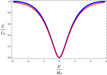
Figure 9.1: Comparison between the Higgs-Dilaton inflationary potential (blue continuous line) obtained from (9.22) in the scale-invariant region and the corresponding one for the Higgs Inflation model (red dotted line). The amplitudes are normalized to the asymptotic value $U_{0}=\frac{\lambda M_{P}^{4}}{4\xi_{h}^{2}}$.

The potential (9.18) becomes

$$\tilde{U}(\phi)=\frac{\lambda M_{P}^{4}}{4\xi_{h}^{2}(1-\varsigma)^{2}}\left(1-\varsigma\cosh^{2}[a\phi/M_{P}]\right)^{2}\ ,$$ (9.22)

$$\tilde{U}_{\Lambda_{0}}(r,\phi)=\frac{\Lambda_{0}}{\gamma^{4}}\varsigma^{2}\cosh^{4}[a\phi/M_{P}]e^{-4\gamma r/M_{P}}\ ,$$

whose scale-invariant part $\tilde{U}(\phi)$ resembles the potential of the simplest Higgs inflationary scenario [120], see Fig. 9.1. The analytical expressions for the amplitude and the spectral tilt of scalar perturbations at order $\mathcal{O}(\xi_{\chi},1/\xi_{h},1/N^{*})$ can be easily calculated to obtain [144]

$$P_{\zeta}(k_{0})\simeq\frac{\lambda\sinh^{2}[4\xi_{\chi}N^{*}]}{1152\pi^{2}\xi_{\chi}^{2}\xi_{h}^{2}}\ ,\hskip 28.45274ptn_{s}(k_{0})\simeq 1-8\xi_{\chi}\coth(4\xi_{\chi}N^{*})\ ,$$ (9.23)

where $N^{*}$ denotes the number of e-folds between the moment at which the pivot scale $k_{0}/a_{0}=0.002\ \text{Mpc}^{-1}$ exited the horizon and the end of inflation. Note that for $1<4\xi_{\chi}N^{*}\ll 4N^{*}$, the expression for the tilt simplifies and becomes linear in $\xi_{\chi}$

$$n_{s}(k_{0})\simeq 1-8\xi_{\chi}\ .$$ (9.24)

An interesting cosmological phenomenology arises with the peculiar choice $\beta=0$. In this case, the DE dominated period in the late Universe depends only on the dilaton field $\rho$, which give rise to an intriguing relation between the inflationary and DE domination periods. Let us start by noticing that around the minimum of the potential the value of $\theta$ is very close to zero. In that limit, $\tan^{2}\theta\ll\eta$, which prevents the use of the field redefinition (9.19). The appropriate redefinitions needed to diagonalize the kinetic term (9.16) in this case turn out to be

$$r=\gamma^{-1}\rho\ \ \ \text{and}\ \ \ \phi^{\prime}\simeq\frac{M_{P}}{\sqrt{\xi_{h}\varsigma}}\theta\ .$$ (9.25)

Using (9.16) and (9.18), it is straightforward to show that the part of the theory associated to the Higgs field $\phi$ simplifies to the SM one. The resulting scale-invariance breaking potential for the dilaton is still of the “run-away” type

$$\tilde{U}_{\Lambda_{0}}(r)=\frac{\Lambda_{0}}{\gamma^{4}}e^{-4\gamma r/M_{P}}\ ,$$ (9.26)

making it suitable for playing the role of quintessence. Let us assume that $\tilde{U}_{\Lambda_{0}}$ is negligible during the radiation and matter dominated stages but responsible for the present accelerated expansion of the Universe. In that case, it is possible to write the following relation between the equation of state parameter $\omega_{r}$ of the $r$ field and its relative abundance $\Omega_{r}$ [157]

$$1+\omega_{r}=\frac{16\gamma^{2}}{3}\left[\frac{1}{\sqrt{\Omega_{r}}}-\frac{1}{2}\left(\frac{1}{\Omega_{r}}-1\right)\log\frac{1+\sqrt{\Omega_{r}}}{1-\sqrt{\Omega_{r}}}\right]^{2}\ .$$ (9.27)

For the present DE density $\Omega_{\text{DE}}=\Omega_{r}\simeq 0.74$, the above expression yields

$$1+\omega_{\text{DE}}=\frac{8}{3}\frac{\xi_{\chi}}{1+6\xi_{\chi}}\ .$$ (9.28)

Comparing (9.24) and (9.28), it follows that the deviation of the scalar tilt $n_{s}$ from the scale-invariant one is proportional to the deviation of the DE equation of state from a cosmological constant [144]

$$n_{s}-1\simeq-3(1+\omega_{\text{DE}}),\ \ \ \text{for}\ \ \ \frac{2}{3N^{*}}<1+\omega_{\text{DE}}\ll 1\ .$$ (9.29)

The above condition is a non-trivial prediction of Higgs-Dilaton cosmology, relating two a priori completely independent periods in the history of the Universe. This has interesting consequences from an observational point of view and makes the Higgs-Dilaton scenario rather unique. We will be back to this point in Sec. 9.4, where we will show that the consistency relation (9.29) still holds even in the presence of quantum corrections computed within the “minimal setup”.

9.3 The dynamical cut-off scale

Following [154], we now turn to the determination of the energy domain where the Higgs-Dilaton model can be considered as a predictive effective field theory. This domain is bounded from above by the field-dependent cut-off $\Lambda(\Phi)$, i.e. the energy where perturbative tree-level unitarity is violated [158]. At energies above that scale, the theory becomes strongly-coupled and the standard perturbative methods fail. In order to determine this (background dependent) energy scale, two related methods, listed below, can be used.

1. Expand the generic fields of the theory around their background values

   $$\Phi(\mathbf{x},t)=\bar{\Phi}+\delta\Phi(\mathbf{x},t)\ ,$$ (9.30)

   such that all kind of higher-dimensional non-renormalizable operators

   $$c_{n}\frac{\mathcal{O}_{n}(\delta\Phi)}{[\Lambda(\bar{\Phi})]^{n-4}}\ ,$$ (9.31)

   with $c_{n}\sim\mathcal{O}(1)$ appear in the resulting action. These operators are suppressed by appropriate powers of the field-dependent coefficient $\Lambda(\bar{\Phi})$, which can be identified as the cut-off of the theory. This procedure gives us only a lower estimate of the cut-off, since it does not take into account the possible cancelations that might occur between the different scattering diagrams.

2. Calculate at which energy each of the N-particle scattering amplitudes hit the unitarity bound. The cut-off will then be the lowest of these scales.

In what follows we will apply these two methods to determine the effective cut-off of the theory. We will start by applying the method $(1)$ to compute the cut-off associated with the gravitational and scalar interactions. The cut-off associated to the gauge and fermionic sectors will be obtained via the method $(2)$.

9.3.1 Cut-off in the scalar-gravity sector

We choose to work in the original Jordan frame where the Higgs and dilaton fields are non-minimally coupled to gravity. Expanding these fields around a static background

$$g_{\mu\nu}=\bar{g}_{\mu\nu}+\delta g_{\mu\nu}\ ,\hskip 14.22636pt\chi=\bar{\chi}+\delta\chi\ ,\hskip 14.22636pth=\bar{h}+\delta h\ ,$$ (9.32)

we obtain the following kinetic term for the quadratic Lagrangian of the gravity and scalar sectors

$$\mathscr{K}_{2}^{\text{G+S}}=\frac{\xi_{\chi}\bar{\chi}^{2}+\xi_{h}\bar{h}^{2}}{8}\left(\delta g^{\mu\nu}\square\delta g_{\mu\nu}+2\partial_{\nu}\delta g^{\mu\nu}\partial^{\rho}\delta g_{\mu\rho}-2\partial_{\nu}\delta g^{\mu\nu}\partial_{\mu}\delta g\right.$$ (9.33)

$$\left.-\delta g\square\delta g\right)-\frac{1}{2}(\partial\delta\chi)^{2}-\frac{1}{2}(\partial\delta h)^{2}+(\xi_{\chi}\bar{\chi}\delta\chi+\xi_{h}\bar{h}\delta h)(\partial_{\lambda}\partial_{\rho}\delta g^{\lambda\rho}-\square\delta g)\ .$$

The leading higher-order non-renormalizable operators obtained in this way are given by

$$\xi_{\chi}(\delta\chi)^{2}\square\delta g\ ,\ \ \ \xi_{h}(\delta h)^{2}\square\delta g\ .$$ (9.34)

Note that these operators are written in terms of quantum excitations with non-diagonal kinetic terms. In order to properly identify the cut-off of the theory, we should determine the normal modes that diagonalize the quadratic Lagrangian (9.33). After doing that, and using the equations of motion to eliminate artificial degrees of freedom, we find that the metric perturbations depend on the scalar fields perturbations, a fact that is implicit in the Lagrangian (9.33). The gravitational part of the above action can be recast into canonical form in terms of a new metric perturbation $\delta\hat{g}_{\mu\nu}$ given by

$$\delta\hat{g}_{\mu\nu}=\frac{1}{\sqrt{\xi_{\chi}\bar{\chi}^{2}+\xi_{h}\bar{h}^{2}}}\left[(\xi_{\chi}\bar{\chi}^{2}+\xi_{h}\bar{h}^{2})\delta g_{\mu\nu}+2\bar{g}_{\mu\nu}(\xi_{\chi}\bar{\chi}\delta\chi+\xi_{h}\bar{h}\delta h)\right]\ .$$ (9.35)

The cut-off scale associated to purely gravitational interactions becomes in this way the effective Planck scale in the Jordan frame

$$\Lambda_{P}^{2}=\xi_{\chi}\bar{\chi}^{2}+\xi_{h}\bar{h}^{2}\ .$$ (9.36)

The remaining non-diagonal kinetic term for the scalar perturbations
$(\delta\Phi^{1},\delta\Phi^{2})=(\delta h,\delta\chi)$ is given in compact matrix notation by

$$\mathscr{K}_{2}^{\text{S}}=-\frac{1}{2}\bar{\kappa}^{J}_{ij}\partial_{\mu}\delta\Phi^{i}\partial^{\mu}\delta\Phi^{j}\ ,$$ (9.37)

where $\bar{\kappa}^{J}_{ij}=\Omega^{2}\bar{\kappa}^{E}_{ij}$ is the Jordan frame analogue of (9.14) and depends only on the background values of the fields, i.e.

$$\bar{\kappa}^{J}_{ij}=\frac{1}{\xi_{\chi}\bar{\chi}^{2}+\xi_{h}\bar{h}^{2}}\begin{pmatrix}\xi_{\chi}\bar{\chi}^{2}(1+6\xi_{\chi})+\xi_{h}\bar{h}^{2}&6\xi_{\chi}\bar{\chi}\xi_{h}\bar{h}\\ 6\xi_{\chi}\bar{\chi}\xi_{h}\bar{h}&\xi_{\chi}\bar{\chi}^{2}+\xi_{h}\bar{h}^{2}(1+6\xi_{h})\end{pmatrix}\ .$$ (9.38)

In order to diagonalize the above expression we make use of the following set of variables

$$\delta\hat{\chi}=\sqrt{\frac{\xi_{\chi}\bar{\chi}^{2}(1+6\xi_{\chi})+\xi_{h}\bar{h}^{2}(1+6\xi_{h})}{(\xi_{\chi}^{2}\bar{\chi}^{2}+\xi_{h}^{2}\bar{h}^{2})(\xi_{\chi}\bar{\chi}^{2}+\xi_{h}\bar{h}^{2})}}\left(\xi_{\chi}\bar{\chi}\delta\chi+\xi_{h}\bar{h}\delta h\right)\ ,$$ (9.39)

$$\delta\hat{h}=\frac{1}{\sqrt{\xi_{\chi}^{2}\bar{\chi}^{2}+\xi_{h}^{2}\bar{h}^{2}}}\left(-\xi_{h}\bar{h}\delta\chi+\xi_{\chi}\bar{\chi}\delta h\right)\ .$$

Note here that this is precisely the change of variables (up to an appropriate rescaling with the conformal factor $\Omega$) needed to diagonalize the kinetic terms for the scalar perturbations in the Einstein frame. To see this, it is enough to start from (9.13) and expand the fields around their background values $\Phi^{i}\rightarrow\bar{\Phi}^{i}+\delta\Phi^{i}$. Keeping the terms with the lowest power in the excitations, $\tilde{K}=\bar{\kappa}^{E}_{ij}\partial_{\mu}\delta\Phi^{i}\partial^{\mu}\delta\Phi^{j}+\mathcal{O}(\delta\Phi^{3})$, it is straightforward to show that the previous expression can be diagonalized in terms of

$$\delta\hat{\chi}=\bar{\Omega}^{-1}\sqrt{\frac{\xi_{\chi}\bar{\chi}^{2}(1+6\xi_{\chi})+\xi_{h}\bar{h}^{2}(1+6\xi_{h})}{(\xi_{\chi}^{2}\bar{\chi}^{2}+\xi_{h}^{2}\bar{h}^{2})(\xi_{\chi}\bar{\chi}^{2}+\xi_{h}\bar{h}^{2})}}\left(\xi_{\chi}\bar{\chi}\delta\chi+\xi_{h}\bar{h}\delta h\right)\ ,$$ (9.40)

$$\delta\hat{h}=\bar{\Omega}^{-1}\frac{1}{\sqrt{\xi_{\chi}^{2}\bar{\chi}^{2}+\xi_{h}^{2}\bar{h}^{2}}}\left(-\xi_{h}\bar{h}\delta\chi+\xi_{\chi}\bar{\chi}\delta h\right)\ .$$

Written in terms of the canonically normalized variables (9.35) and (9.39) these operators read

$$\frac{1}{\Lambda_{1}}(\delta\hat{h})^{2}\square\delta\hat{g}\ ,\ \ \ \frac{1}{\Lambda_{2}}(\delta\hat{\chi})^{2}\square\delta\hat{g}\ ,\ \ \ \frac{1}{\Lambda_{3}}(\delta\hat{\chi})(\delta\hat{h})\square\delta\hat{g}\ ,$$ (9.41)

where the different cut-off scales are given by

$$\centering\Lambda_{1}\@add@centering =\frac{\xi_{\chi}^{2}\bar{\chi}^{2}+\xi_{h}^{2}\bar{h}^{2}}{\xi_{\chi}\xi_{h}\sqrt{\xi_{\chi}\bar{\chi}^{2}+\xi_{h}\bar{h}^{2}}}\ ,$$ (9.42)

$$\Lambda_{2} =\frac{(\xi_{\chi}^{2}\bar{\chi}^{2}+\xi_{h}^{2}\bar{h}^{2})(\xi_{\chi}\bar{\chi}^{2}(1+6\xi_{\chi})+\xi_{h}\bar{h}^{2}(1+6\xi_{h}))}{(\xi_{\chi}^{3}\bar{\chi}^{2}+\xi_{h}^{3}\bar{h}^{2})\sqrt{\xi_{\chi}\bar{\chi}^{2}+\xi_{h}\bar{h}^{2}}}\ ,$$ (9.43)

$$\Lambda_{3} =\frac{(\xi_{\chi}^{2}\bar{\chi}^{2}+\xi_{h}^{2}\bar{h}^{2})(\xi_{\chi}\bar{\chi}^{2}(1+6\xi_{\chi})+\xi_{h}\bar{h}^{2}(1+6\xi_{h}))}{\xi_{\chi}\bar{\chi}\xi_{h}\bar{h}\left|\xi_{h}-\xi_{\chi}\right|\sqrt{\xi_{\chi}\bar{\chi}^{2}+\xi_{h}\bar{h}^{2}}}\ .$$ (9.44)

The effective cut-off of the scalar theory at a given value of the background fields will be the lowest of the previous scales. We will be back to this point in Sec. 9.3.3.

9.3.2 Cut-off in the gauge and fermionic sectors

Let us now move to the cut-off associated with the gauge sector. Since we are working in the unitary gauge for the SM fields, it is sufficient to look at the tree-level scattering of non-abelian vector fields with longitudinal polarization. It is well known that in the SM the “good” high energy behaviour of these processes is the result of cancellations that occur when we take into account the interactions of the gauge bosons with the excitations $\delta h$ of the Higgs field  [159, 160].

In our case, even though purely gauge interactions remain unchanged, the graphs involving the Higgs field excitations are modified due to the non-canonical kinetic term. This changes the pattern of the cancellations that occur in the standard Higgs mechanism, altering therefore the asymptotic behaviour of these processes. As a result, the energy scale where this part of the theory becomes strongly coupled becomes lower.

To illustrate how this happens, let us consider the $W_{L}W_{L}\rightarrow W_{L}W_{L}$ scattering in the $s-$channel. The relevant part of the Lagrangian is

$$g\,m_{W}W_{\mu}^{+}W^{-\mu}\delta h\ ,$$ (9.45)

where $m_{W}\sim g\bar{h}$. After diagonalizing the kinetic term for the scalar fields with the change of variables (9.39), the above expression becomes

$$g^{\prime}m_{W}W_{\mu}^{+}W^{-\mu}\delta\hat{h}+g^{\prime\prime}m_{W}W_{\mu}^{+}W^{-\mu}\delta\hat{\chi}\ ,$$ (9.46)

where the effective coupling constants $g^{\prime}\ \text{and}\ g^{\prime\prime}$ are given by

$$g^{\prime}=g\frac{\xi_{\chi}\bar{\chi}}{\sqrt{\xi_{\chi}^{2}\bar{\chi}^{2}+\xi_{h}^{2}\bar{h}^{2}}}\ ,$$ (9.47)

$$g^{\prime\prime}=g\frac{\xi_{h}\bar{h}}{\sqrt{\xi_{\chi}^{2}\bar{\chi}^{2}+\xi_{h}^{2}\bar{h}^{2}}}\sqrt{\frac{\xi_{\chi}\bar{\chi}^{2}+\xi_{h}\bar{h}^{2}}{\xi_{\chi}\bar{\chi}^{2}(1+6\xi_{\chi})+\xi_{h}\bar{h}^{2}(1+6\xi_{h})}}\ .$$

From the requirement of tree unitarity of the $S$-matrix, it is straightforward to show that the scattering amplitude of this interaction hits the perturbative unitarity bound at energies

$$\Lambda_{G}\simeq\sqrt{\frac{\xi_{\chi}\bar{\chi}^{2}(1+6\xi_{\chi})+\xi_{h}\bar{h}^{2}(1+6\xi_{h})}{6\xi_{h}^{2}}}\ .$$ (9.48)

It is interesting to compare the previous expression with the results for the gauge cut-off of the simplest Higgs inflationary model [154]. In order to do that, let us consider two limiting cases: the inflationary/high-energy period corresponding to field values $\xi_{\chi}\chi^{2}\ll\xi_{h}h^{2}$ and the low-energy regime at which $\xi_{\chi}\chi^{2}\gg\xi_{h}h^{2}$ . In these two cases, the above expression simplifies to

$$\Lambda_{G}\simeq\Bigg{\{}\begin{array}[]{cl}\bar{h}&\mbox{for}\ \xi_{\chi}\bar{\chi}^{2}\ll\xi_{h}\bar{h}^{2}\ ,\\ \frac{\sqrt{\xi_{\chi}}\bar{\chi}}{\xi_{h}}&\mbox{for}\ \xi_{\chi}\bar{\chi}^{2}\gg\xi_{h}\bar{h}^{2}\ ,\\ \end{array}$$ (9.49)

in agreement with the Higgs inflation model.

To identify the cut-off of the fermionic part of the Higgs-Dilaton model, we consider the chirality non-conserving process $\bar{f}f\rightarrow W_{L}W_{L}$. This interaction receives contributions from diagrams with $\gamma$ and $Z$ exchange ($s-$channel) and from a diagram with fermion exchange ($t-$channel). In the asymptotic high-energy limit, the total amplitude of these graphs grows linearly with the energy at the center of mass. Once again, the $s-$channel diagram including the Higgs excitations unitarizes the associated amplitude [161, 162, 163]. Following therefore the same steps as in the calculation of the gauge cut-off, we find that this part of the theory enters into the strong-coupling regime at energies

$$\Lambda_{F}\simeq y^{-1}\frac{\xi_{\chi}\bar{\chi}^{2}(1+6\xi_{\chi})+\xi_{h}\bar{h}^{2}(1+6\xi_{h})}{6\xi_{h}^{2}\bar{h}}\ ,$$ (9.50)

where $y$ is the Yukawa coupling constant. The above cut-off is higher than that of the SM gauge interactions (9.48) during the whole evolution of the Universe.

9.3.3 Comparison with the energy scales in the early and late Universe

In this section we compare the cut-offs found above with the characteristic energy scales in the different periods during the evolution of the Universe. If the typical momenta involved in the different processes are sufficiently small, the theory will remain in the weak coupling limit, making the Higgs-Dilaton scenario self-consistent.

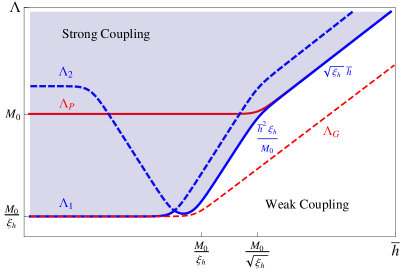
Figure 9.2: Dependence of the different cut-off scales for a fixed value of the dilaton field $\bar{\chi}$ as a function of the Higgs field $\bar{h}$ in the Jordan frame. The cut-off (9.44) is parametrically above the other energy scales ($\Lambda_{1},\ \Lambda_{2},\ \Lambda_{P},\ \Lambda_{G}\ \text{and}\ \Lambda_{F}$) during the whole history and it is therefore not included in the figure. The effective field theory description of scalar fields is applicable for typical energies below the thick blue solid line, which correspond to the minimum of the scalar cut-off scales at a given field value. This is given by $\Lambda_{2}$ and $\Lambda_{1}$ in the scalar sector, for large and small Higgs values respectively. The red solid line correspond to the gravitational cut-off (9.36), while the red dashed one corresponds to the gauge cut-off (9.48). They coincide with the effective scalar cut-off for the limiting values of the Higgs field. The scale $M_{0}$ is defined as $M_{0}=\sqrt{\xi_{\chi}}\bar{\chi}$ and corresponds to the value of the effective Planck mass at low energies.

Let us start by considering the inflationary period, characterized by $\xi_{h}\bar{h}^{2}\gg\xi_{\chi}\bar{\chi}^{2}$. As shown in Fig. 9.2, the lowest cut-off in this region is the one associated with the gauge interactions $\Lambda_{G}$. The typical momenta of the scalar perturbations produced during inflation are of the order of the Hubble parameter at that time. This quantity can be easily estimated in the Einstein frame, where it is basically determined by the energy stored in the inflationary potential (9.22). We obtain $\tilde{H}\sim\sqrt{\lambda}M_{P}/\xi_{h}$. When transformed to the Jordan frame ($H=\Omega\tilde{H}$) this quantity becomes $H\sim\sqrt{\frac{\lambda}{\xi_{h}}}\bar{h}$, which is significantly below the cut-off scale $\Lambda_{G}$ in that region. The same conclusion is obtained for the total energy density, which turns out to be much smaller than $\Lambda_{G}^{4}$. Moreover, the cut-off $\Lambda_{G}$ exceeds the masses of all particles in the Higgs background, allowing a self-consistent estimate of radiative corrections (see Sec. 9.4).

After the end of inflation, the field $\phi$ starts to oscillate around the minimum of the potential with a decreasing amplitude, due to the expansion of the Universe and particle production. This amplitude varies between $M_{0}/\sqrt{\xi_{h}}$ and $M_{0}/\xi_{h}$, where $M_{0}=\sqrt{\xi_{\chi}}\bar{\chi}$ is the asymptotic Planck scale in the low energy regime. As shown in Fig. 9.1, the curvature of the Higgs-Dilaton potential around the minimum coincides (up to ${\cal{O}}(\xi_{\chi})$ corrections) with that of the Higgs-inflation scenario. All the relevant physical scales, including the effective gauge and fermion masses, agree, up to small corrections, with those in Higgs-inflation [164] . This allows us to directly apply the results of [121, 122, 165] to the Higgs-Dilaton scenario. According to these works, the typical momenta of the gauge bosons produced at the minimum of the potential in the Einstein frame is of order $\tilde{k}\sim(\tilde{m}_{A}/M)^{2/3}M$, with $\tilde{m}_{A}$ the mass of the gauge bosons in the Einstein frame and $M=\sqrt{\lambda/3}M_{P}/\xi_{h}$ the curvature of the potential around the minimum. After transforming to the Jordan frame we obtain $k\sim\left(\frac{\lambda g^{4}}{\xi_{h}}\right)^{1/6}\Lambda_{G}$, with $g$ the weak coupling constant. The typical momentum of the created gauge bosons is therefore parametrically below the gauge cut-off scale (H.4) in that region.

At the end of the reheating period, $\xi_{\chi}\bar{\chi}^{2}\gg\xi_{h}\bar{h}^{2}$, the system settles down to the minimum of the potential $\tilde{U}(\phi)$, see (9.22). In that region the effective Planck mass coincides with the value $M_{0}$. The cut-off scale becomes $\Lambda_{1}\simeq\sqrt{\xi_{\chi}}\bar{\chi}/\xi_{h}\simeq M_{P}/\xi_{h}$. This value is much higher than the electroweak scale $m_{H}^{2}\sim 2\alpha/\xi_{\chi}M_{P}$ (see (9.4)) where all the physical processes take place. We conclude therefore that perturbative unitarity is maintained for all the relevant processes during the whole evolution of the Universe.

9.4 Quantum corrections

In this section we concentrate on the radiative corrections to the inflationary potential and on their influence on the predictions of the model.

Our strategy is as follows. We regularize the quantum theory in such a way that all multi-loop diagrams are finite, whereas the exact symmetries of the chosen classical action (gauge, diffeomorphisms and scale invariance) remain intact. Moreover, we will require the regularization to respect the approximate shift symmetry of the dilaton field in the Jordan frame, see Sec. 9.2. Then we add to the classical action an infinite number of counter-terms (including the finite parts as well) which remove all the divergences from the theory and do not spoil the exact and approximate symmetries of the classical action. Since the theory is not renormalizable, these counter-terms will have a different structure from that of the classical action. In particular, terms that are non-analytic with respect to the Higgs and dilaton fields will appear [166]. They can be considered as higher-dimensional operators, suppressed by the field-dependent cut-offs. For consistency with the analysis made earlier in this work, we demand these cut-offs to exceed those found in Sec. 9.3.

An example of the subtraction procedure which satisfies all the requirements formulated above has been constructed in [9] (see also earlier discussion in [8]). It is based on dimensional regularization in which the ’t Hooft-Veltman normalization point $\mu$ is replaced by some combination of the scalar fields with an appropriate dimension, $\mu^{2}\to F(\chi,h)$ (we underline that we use the Jordan frame here for all definitions). The infinite part of the counter-terms is defined as in $\overline{MS}$ prescription, i.e. by subtracting the pole terms in $\epsilon$, where the dimensionality of space-time is $D=4-2\epsilon$. The finite part of the counter-terms has the same operator structure as the infinite part, including the parametric dependence on the coupling constants.

Although the requirement of the structure of higher-dimensional operators, formulated in the previous paragraphs puts important constraints on the function $F(\chi,h)$, its precise form is not completely determined [9, 166, 167], and the physical results do depend on the choice of $F(\chi,h)$. This somewhat mysterious fact from the point of view of uniquely defined classical theory (9.1) becomes clear if we recall that we are dealing with a non-renormalizable theory. The quantization of this kind of theories requires the choice of a particular classical action together with a set of subtraction rules. The ambiguity in the choice of the field-dependent normalization point $F(\chi,h)$ simply reflects our ignorance about the proper set of rules. Different subtractions prescriptions applied to the same classical action do produce unequal results. Sometimes this ambiguity is formulated as a dependence of quantum theory on the choice of conformally related frames in scalar-tensor theories [168]. The use of the same quantization rules in different frames would lead to quantum theories with different choices of $F(\chi,h)$.

Among the many possibilities, the simplest and most natural choice is to identify the normalization point in the Jordan frame with the gravitational cut-off (9.36),

$$\mu_{I}^{2}\propto\xi_{\chi}\chi^{2}+\xi_{h}h^{2},$$ (9.51)

which corresponds to the scale-invariant prescription of [9]. In the Einstein frame the previous choice becomes standard (field-independent)

$$\tilde{\mu}_{I}^{2}\propto M_{P}^{2}\,.$$ (9.52)

A second possibility is to choose the scale-invariant direction along the dilaton field, i.e.

$$\mu_{II}^{2}\propto\xi_{\chi}\chi^{2}.$$ (9.53)

When transformed to the Einstein frame it becomes

$$\tilde{\mu}_{II}^{2}\propto\frac{\xi_{\chi}\chi^{2}M_{P}^{2}}{\xi_{\chi}\chi^{2}+\xi_{h}h^{2}}\,,$$ (9.54)

and coincides with the prescription II of [126] at the end of inflation.

In what follows we will use this “minimal setup" for the analysis of the radiative corrections. It will be more convenient to work in the Einstein frame, where the coupling to gravity is minimal and all non-linearities are moved to the matter sector. The total action in the Einstein frame naturally divides into an Einstein- Hilbert (EH) part, a purely scalar piece involving only the Higgs and dilaton (HD) fields and a part corresponding to the chiral SM (CH) without the radial mode of the Higgs boson [126, 169, 170]

$$S=S_{\text{EH}}+S_{\text{HD}}+S_{\text{CH}}\,.$$ (9.55)

In the next section we estimate the contribution of the scalar sector to the effective inflationary potential, postponing the study of the chiral SM to Sec. 9.4.2. All the computations will be performed in flat spacetime, since the inclusion of gravity does not modify the results .

9.4.1 Scalar contribution to the effective inflationary potential

Let us start by reminding that the initial value of the dilaton field has to be sufficiently large to keep its present contribution to DE at the appropriate observational level [144]. The latter fact allows us to neglect the exponentially suppressed contributions to the effective action stemming from $\tilde{U}_{\Lambda_{0}}$ in (9.22). As a result, the remaining corrections due to the dilaton field will emerge from its non-canonical kinetic term, whereas all the radiative corrections due to the Higgs field will emerge from the inflationary potential.

The construction of the effective action for the scalar sector of the theory is most easily done in the following way: expand the action (9.21) near the constant background of the dilaton and the Higgs fields and drop the linear terms in perturbations. After that, compute all the vacuum diagrams to account for the potential-type corrections and all the diagrams with external legs to account for the kinetic-type corrections.

Dilaton contribution

Let us consider first the quantum corrections to the dilaton itself. Since our subtraction procedure respects the symmetries of the classical action (in particular scale invariance, corresponding to the shift symmetry of the dilaton field $r$ in the Einstein frame), no potential terms for the dilaton can be generated. Thus, the loop expansion can only create two types of contributions, both stemming from its kinetic term. The first type are corrections to the propagator of the field, and as we will show below they are effectively controlled by $(m_{H}/M_{P})^{2k}$, with $m_{H}^{2}\equiv-\tilde{U}^{\prime\prime}(\phi)$ and $k$ the number of loops under consideration. The second type are operators with more derivatives of the field suppressed by appropriate powers of the scalar cut-off $M_{P}$. One should bear in mind that the appearance of these operators in the effective action is expected and consistent. As discussed in the previous section, their presence does not affect the dynamics of the model, since the scalar cut-off is much larger than the characteristic momenta of the particles involved in all physical processes throughout the whole history of the Universe.

To demonstrate explicitly what we described above, let us consider some of the associated diagrams. Following the ideas of [9], we perform the computations in dimensional regularization in $D=4-2\epsilon$ dimensions. We avoid therefore the use of other regularizations schemes, such as cut-off regularization, where the scale invariance of the theory is badly broken at tree level. The magnitude of the corrections in dimensional regularization is of the order of the masses of the particles running in the loops, or in the case of the massless dilaton, its momentum. The structure of the corrections can be therefore guessed by simple power-counting and it becomes apparent already at the one-loop order. We get

where

the Higgs and dilaton fields are represented by solid and dashed lines respectively. To keep the expressions as compact as possible we set $1/\bar{\epsilon}=1/\epsilon-\gamma+\log 4\pi$ and denoted by $f\ \text{and}\ f^{\prime}$ the finite parts of the diagrams, whose values depend on the normalization point $\mu$. The higher-derivative operator in the second diagram is included for completion, but turns out to vanish accidentally in this particular case. Numerical factors are absorbed into the background-dependent coefficients $c_{k,V}^{d_{i}}(\bar{\phi})$, which depend on the particular diagram $d_{i}$ under consideration, the number of loops $k$ and the number of vertices $V$. Their values are always smaller than unity, and vary slightly with the background value $\bar{\phi}$. Their specific form of is presented in the Appendix I.

In two-loops the situation is somehow similar. The divergent (and finite) part of the corrections (consider for example the diagrams presented in Fig. 9.3) is proportional to

$$c_{2,V}^{d_{i}}(\bar{\phi})\left[\left(\dfrac{m_{H}}{M_{P}}\right)^{4}+\left(\dfrac{m_{H}}{M_{P}}\right)^{2}\left(\dfrac{\partial}{M_{P}}\right)^{2}+\left(\dfrac{\partial}{M_{P}}\right)^{4}\right](\partial r)^{2}\ ,\ \ \ V\leq 4\ .$$ (9.56)

It is not difficult to convince oneself that this happens in the higher order diagrams as well. The structure of the corrections is therefore proportional to

$$c_{k,V}^{d_{i}}(\bar{\phi}) \left[\left(\dfrac{m_{H}}{M_{P}}\right)^{2k}+\left(\dfrac{m_{H}}{M_{P}}\right)^{2k-2}\left(\dfrac{\partial}{M_{P}}\right)^{2}+\ldots\right.$$ (9.57)

$$\left.+\left(\dfrac{m_{H}}{M_{P}}\right)^{2}\left(\dfrac{\partial}{M_{P}}\right)^{2k-2}+\left(\dfrac{\partial}{M_{P}}\right)^{2k}\right](\partial r)^{2}\ ,$$

up to $\mathcal{O}(1)$ numerical factors. Notice that some operators involving higher derivatives were already present at lower orders, but they reappear with extra suppression factors $(m_{H}/M_{P})^{2}$ on top of the scalar cut-off $M_{P}$. The corrections from diagrams with gauge bosons and fermions running inside the loops are given also by (9.57), by consistently replacing $m_{H}$ by the mass of the particle considered.

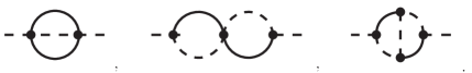
Figure 9.3: Some of the two-loop diagrams for the dilaton.

Higgs contribution

We now turn to the corrections to the Higgs field. Once again we consider first the potential-type contributions. The situation now is more complicated, since the effective potential for the Higgs field $\phi$ will be modified by terms stemming from the scale-invariant part of the tree-level potential (9.22) as well as from the non-canonical kinetic term of the dilaton field $r$, with the latter starting from the second order in perturbation theory.

Let us start by considering the contributions due to the tree-level potential. To keep the notation as simple as possible, we express the scale-invariant part of the potential (9.22) in the following compact form

$$\tilde{U}(\phi)=\lambda U_{0}\left(u_{0}+\sum_{n=1}^{2}u_{n}\cosh[2na\phi/M_{P}]\right),\hskip 14.22636ptU_{0}=\frac{M_{P}^{4}}{4\xi_{h}^{2}(1-\varsigma)^{2}}\ ,$$ (9.58)

where, for completion, we have explicitly recovered the $\alpha$ and $\beta$ dependence and defined

$$u_{0}=c^{2}-c\sigma+\frac{3\sigma^{2}}{8}+\frac{3\beta^{\prime}}{2}\ ,\ u_{1}=\frac{\sigma^{2}}{2}-c\sigma-2\beta^{\prime}\ ,\ u_{2}=\frac{\sigma^{2}}{8}+\frac{\beta^{\prime}}{2}\ ,$$ (9.59)

with

$$c=1+\frac{\alpha}{\lambda}\frac{1+6\xi_{h}}{1+6\xi_{\chi}}\ ,\ \ \ \sigma=\varsigma+\frac{\alpha}{\lambda}\frac{1+6\xi_{h}}{1+6\xi_{\chi}}\ ,\ \ \ \ \beta^{\prime}\equiv\frac{\beta}{\lambda}\left(\frac{1+6\xi_{h}}{1+6\xi_{\chi}}\right)^{2}\ .$$ (9.60)

Expanding the field around its background value $\bar{\phi}$, we get

$$\tilde{U}(\bar{\phi}+\delta\phi) =\lambda U_{0}\sum_{n=1}^{2}u_{n}\sum_{l=0}^{\infty}\frac{\cosh^{(l)}[2na\bar{\phi}/M_{P}]}{l!}\left(\frac{2na\delta\phi}{M_{P}}\right)^{l}$$ (9.61)

$$=\lambda U_{0}\sum_{n=1}^{2}\sum_{l=0}^{\infty}u_{n}\left[c_{n,l}\cosh[2na\bar{\phi}/M_{P}]\left(\frac{a\delta\phi}{M_{P}}\right)^{2l}\right.$$

$$\left.+d_{n,l}\sinh[2na\bar{\phi}/M_{P}]\left(\frac{a\delta\phi}{M_{P}}\right)^{2l+1}\right]\ ,$$

where $c_{n,l}\ \text{and}\ d_{n,l}$ account for numerical coefficients and combinatorial factors. Since the theory is non-renormalizable, the perturbative expansion creates terms which do not have the same background dependence of the original potential. Up to numerical factors, the contributions turn out to be of the form

$$\frac{\lambda^{i+j}M_{P}^{4}}{[4\xi_{h}^{2}(1-\varsigma)^{2}]^{i+j}}\left[g\left(\frac{1}{\epsilon}\right)+f_{i,j}\right]\sum_{n,m}u_{n}^{i}u_{m}^{j}\cosh^{i}[2na\bar{\phi}/M_{P}]\sinh^{j}[2ma\bar{\phi}/M_{P}]\ ,$$ (9.62)

where $f_{i,j}$ denotes the (finite) integration constant, and $g(1/\epsilon)$ is a function of the divergent terms. Note that if we set $\beta=0$, we make sure that terms which contribute to the cosmological constant (9.5) will not be generated by the loop expansion.

By inspection of the structure of divergences, we can see that the leading corrections are those appearing with the lowest power in $\varsigma$. To gain insight on their contribution, we calculate the finite part of (9.62) for the maximal value of the hyperbolic functions. This corresponds to $\phi_{\text{max}}=\phi_{0}\equiv M_{P}/a\ \tanh^{-1}[\sqrt{1-\varsigma}]$. We get

$$\frac{\lambda^{i+j}}{[4\xi_{h}^{2}(1-\varsigma)^{2}]^{i+j}}f_{i,j}\times$$ (9.63)

$$\times\sum_{n,m}u_{n}^{i}u_{m}^{j}\cosh^{i}[2na\bar{\phi}/M_{P}]\sinh^{j}[2ma\bar{\phi}/M_{P}]\Big{|}_{\bar{\phi}=\phi_{\text{max}}}\sim\left(\frac{\lambda\varsigma}{4\xi_{h}^{2}}\right)^{i+j}f_{i,j}\ ,$$

which makes the corrections coming from the order $i+j+1$ negligible compared to the ones from $i+j$ order. In the last step we have simply set $c=1,\ \sigma=\varsigma$, which, given the small value of the parameter $\alpha$ appearing in (9.60), constitutes a very good approximation.

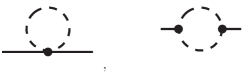
(a)

(b)

Figure 9.4: Characteristic diagrams produced by the non-canonical kinetic term of the dilaton field $r$. Solid and dashed lines represent the Higgs and dilaton fields respectively. The first one-loop diagram presented in (a) vanishes in dimensional regularization due to the massless character of the dilaton field. On the other hand, the second diagram gives rise to higher derivative terms of the Higgs field. In (b) we consider two and three loop diagrams which, apart from generating higher dimensional operators, contribute to the effective potential once we amputate them.

As we mentioned earlier, potential-type corrections to the Higgs field are also generated from diagrams associated to the kinetic term of the dilaton $r$, starting from two loops. This happens because the first order vacuum diagrams with dilaton running in the loop, vanish. If we consider higher loop diagrams, like those in Fig. 9.4(b) but without momenta in the external legs, we see that even though the background dependence of the corrections is complicated due to the non-canonically normalized dilaton that runs inside the loops, their contributions to the effective action are of the same order as those in (9.63).

We now turn to the kinetic-type corrections to the Higgs field. By that we mean corrections to the propagator, as well as terms with more derivatives of the field suppressed by the scalar cut-off. The first type of contributions come only from the scale-invariant part of the potential given by (9.58) , when the momenta associated to the external legs are considered. It is not difficult to show that these are precisely of the same form as those in (9.62). The second type of contributions, i.e. the higher dimensional operators, are generated both from the Higgs potential at higher loops, as well as from the non-vanishing diagrams associated to the non-canonical kinetic term of the dilaton. The terms we get are proportional to

$$\frac{\partial^{2}}{M_{P}^{2}}(\partial\phi)^{2}\ ,\ \ \ \frac{\partial^{4}}{M_{P}^{4}}(\partial\phi)^{2}\ \ldots\,,$$ (9.64)

and they can be safely neglected for the typical momenta involved in the different epochs of the evolution of the Universe.

Before moving on, we would like to comment on the appearance of mixing terms with derivatives of the fields. These manifest themselves when we consider diagrams with both fields in the external legs. They are higher dimensional operators, and it can be shown that they appear suppressed by the scalar cut-off of the theory, as before.

Since the kinetic-type operators do not modify the dynamics, we will consider only potential-type corrections to estimate the change in the tree-level predictions of the model. At one-loop, the contribution of the scalar sector to the inflationary potential becomes [172]

$$\Delta\tilde{U}_{HD} \simeq\frac{U_{0}}{64\pi^{2}}\frac{\lambda a^{4}}{\xi_{h}^{2}(1-\varsigma)^{2}}\left(\frac{1}{\bar{\epsilon}}+f_{2,0}\right)\left[\varsigma^{2}\frac{1+\cosh[4a\bar{\phi}/M_{P}]}{2}+\mathcal{O}(\varsigma^{3})\right]\ ,$$ (9.65)

where we just kept the leading contribution in $\varsigma$. The finite part $f_{2,0}$ in the previous expression is given by

$$f_{2,0} =\frac{3}{2}-\log\left[\frac{-\tilde{U}^{\prime\prime}(\bar{\phi})}{\mu^{2}}\right]$$ (9.66)

$$=\frac{3}{2}-\log\left[\frac{\lambda a^{2}M_{P}^{2}}{\xi_{h}^{2}(1-\varsigma)^{2}\mu^{2}}\Bigg{(}\varsigma\cosh[2a\bar{\phi}/M_{P}]+\mathcal{O}(\varsigma^{2})\Bigg{)}\right]\ .$$

If we adopt the $\overline{MS}$ scheme, the remaining (logarithmic) corrections will be suppressed by an overall factor $\mathcal{O}(10^{-15})$ (apart from different powers of $\varsigma$) with respect to the tree-level potential (9.58). The quantum contribution of the scalar sector to the effective inflationary potential is therefore completely negligible and rather insensitive to the particular choice of the renormalization point $\mu$. This allows us to approximate the value of $\phi$ at the end of inflation by its classical value $\phi_{f}\simeq M_{P}/a\ \tanh^{-1}\left[\sqrt{1-\varsigma}\cos(2\times 3^{1/4}\sqrt{\xi_{\chi}})\right]$, and compute analytically the spectral tilt $n_{s}$ of primordial scalar perturbations, which turns out to be

$$n_{s}(k_{0})-1\simeq-8\xi_{\chi}+\frac{\lambda\xi_{\chi}^{2}}{96\pi^{2}\xi_{h}^{2}}f_{2,0}\ ,\ \ \ \text{for}\ \ \ 1\lesssim 4\xi_{\chi}N^{*}\ll 4N^{*}\ .$$ (9.67)

We see therefore that the correction to the tree-level result is controlled by the effective self-coupling of the Higgs field in the Einstein frame $\lambda/\xi_{h}^{2}$. The small value of this parameter makes the scalar radiative contribution completely negligible and thus hardly modify the consistency relation (9.29). Note however that there might be still a significant contribution to the inflationary potential coming from the SM particles, especially from those with a large coupling to the Higgs field. The study of this effect is the purpose of the next section.

9.4.2 Chiral SM contribution to the effective inflationary potential.

The action for the SM fields during the inflationary stage is similar to that appearing in Higgs inflation [126] and takes the form of a chiral SM with a nearly decoupled Higgs field. Its contribution to the effective potential can be analyzed by the methods presented in [126]. The one-loop contribution during inflation reads

$$\Delta U_{1}=\frac{6m_{W}^{4}}{64\pi^{2}}\left(\log\frac{m_{W}^{2}}{\mu^{2}}-\frac{5}{6}\right)+\frac{3m_{Z}^{4}}{64\pi^{2}}\left(\log\frac{m_{Z}^{2}}{\mu^{2}}-\frac{5}{6}\right)-\frac{3m_{t}^{4}}{16\pi^{2}}\left(\log\frac{m_{t}^{2}}{\mu^{2}}-\frac{3}{2}\right)\ ,$$ (9.68)

where $m_{W}^{2}=g^{2}h^{2}/2$, $m_{Z}^{2}=g^{2}h^{2}/2\cos^{2}\theta_{W}$ and $m_{t}^{2}=y_{t}^{2}h^{2}/2$ stand for the effective $W,Z$ and top quark masses in the Jordan frame. The choice of the $\mu$ parameter here defines the renormalization prescription, as described in the beginning of Sec. 9.4. To retain the possibility to use the RG equations to run between the electroweak and inflationary scales we will write $\mu^{2}=\frac{\hat{\mu}^{2}}{M_{P}^{2}}F(h,\chi)$. Here the function $F(h,\chi)$ corresponds to the choice of the renormalization prescription and leads to different physical results, while the parameter $\hat{\mu}$ plays the role of the usual choice of momentum scale in the RG approach and should disappear in the final result. The conformal transformation to the Einstein frame $\Delta\tilde{U}_{1}=\Delta U_{1}/\Omega^{4}$ acts only on the coefficients of the logarithmic terms in (9.68), leaving their arguments completely unchanged. We obtain therefore

$$\Delta\tilde{U}_{1} =\frac{6\tilde{m}_{W}^{4}}{64\pi^{2}}\left(\log\frac{m_{W}^{2}}{\hat{\mu}^{2}F(h,\chi)/M_{P}^{2}}-\frac{5}{6}\right)+\frac{3\tilde{m}_{Z}^{4}}{64\pi^{2}}\left(\log\frac{m_{Z}^{2}}{\hat{\mu}^{2}F(h,\chi)/M_{P}^{2}}-\frac{5}{6}\right)$$ (9.69)

$$-\frac{3\tilde{m}_{t}^{4}}{16\pi^{2}}\left(\log\frac{m_{t}^{2}}{\hat{\mu}^{2}F(h,\chi)/M_{P}^{2}}-\frac{3}{2}\right)\ ,$$

where the Einstein-frame masses $\tilde{m}^{2}$ are proportional to the effective vacuum expectation value of the Higgs field in the Einstein frame, which is a slowly varying function during inflation,

$$v^{2}(\phi)\equiv\frac{h^{2}}{\Omega^{2}}=\frac{M_{P}^{2}}{\xi_{h}(1-\varsigma)}\left(1-\varsigma\cosh^{2}\frac{a\phi}{M_{p}}\right).$$ (9.70)

This fact allows us to completely factor out the $\phi$ dependence in front of the logarithms in (9.69) and perform the analysis below as if $v$ was a constant, $v\simeq M_{P}/\sqrt{\xi_{h}}$.

Note that the explicit dependence on the ’t Hooft-Veltman normalization point $\hat{\mu}$ in (9.68) is spurious and is compensated by the running of the coupling constants $\lambda(\hat{\mu})$, $\xi_{h}(\hat{\mu})$ in the tree level part of the potential (see [126]). Once the RG running of the couplings is fixed, it is convenient to choose the value of $\hat{\mu}$ in such a way that the logarithmic contribution 9.69, for each given value $\phi$ of the Higgs field, is minimized, $\hat{\mu}^{2}\simeq\frac{y_{t}^{2}}{2}\frac{h^{2}}{F(h,\chi)/M_{P}^{2}}$. In that case, the RG enhanced (RGE) inflationary potential becomes

$$\tilde{U}_{\text{RGE}}(\phi)=\frac{\lambda(\hat{\mu}(\phi))}{4}\frac{M_{P}^{4}}{\xi^{2}_{h}(\hat{\mu}(\phi))(1-\varsigma)^{2}}\left(1-\varsigma\cosh^{2}\frac{a\phi}{M_{p}}\right)^{2}\,,$$ (9.71)

which in fact suffices for practical purposes, with the corrections form the 1-loop logarithms being rather small.

As discussed at the beginning of Sec. 9.4, the different choices of $\mu$ correspond to different subtraction rules and produce different results. In what follows we will consider the two most natural choices. The first one is associated to the scale invariant prescription (9.51). The RG enhancement of the potential in this case dictates

$$\hat{\mu}_{\text{I}}^{2}(\phi)=\frac{y_{t}^{2}}{2}\frac{M_{p}^{2}h^{2}}{\xi_{h}h^{2}+\xi_{\chi}\chi^{2}}=\frac{y_{t}^{2}}{2}v^{2}(\phi)\,,$$ (9.72)

which is nothing else than the effective top mass in the Einstein frame. With this choice, the change in the shape of the potential is very small, given the insignificant variation of $v^{2}(\phi)$ during inflation. The change in the inflationary observables $n_{s}$ and $r$ is therefore expected to be completely negligible. The second possibility that we will consider is associated to the prescription (9.53). In this case the optimal choice of $\hat{\mu}$ is

$$\hat{\mu}^{2}_{\text{II}}(\phi)=\frac{y_{t}^{2}}{2}\frac{M_{P}^{2}h^{2}}{\xi_{\chi}\chi^{2}}=\frac{y_{t}^{2}}{2}v^{2}(\phi)\frac{1-\varsigma}{\varsigma\sinh^{2}\left(a\phi/M_{P}\right)}\,,$$ (9.73)

which, at the end of inflation, coincides with the effective top mass in the Jordan frame. This corresponds to the prescription II in [126]. Note that contrary to the previous case, this choice strongly depends on the value of the $\phi$ field and noticeable contributions to the inflationary parameters are expected.

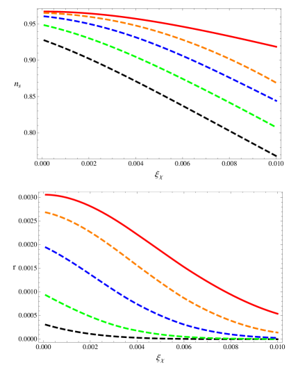
Figure 9.5: The spectral index $n_{s}$ (top) and tensor to scalar ration $r$ (bottom) as a function of the non-minimal coupling $\xi_{\chi}$. The solid line corresponds to the quantization prescription I, which coincides with the tree level result. Dashed lines stand for the quantization choice II for different Higgs masses. The minimal Higgs boson mass $m_{\text{min}}$ can be obtained from [173].

The calculation proceeds now along the same lines as those in [126], using the tree level RG enhanced potential and the one loop correction. The addition of the two loop effective potential does not significantly modify the result. The numerical outcome for the two prescriptions is shown in Fig. 9.5. As expected, the inflationary observables computed with the first prescription coincide with the tree level result. The only effect of the quantum corrections is setting a minimal value for the Higgs mass. This turns out to be $m_{H}>m_{\text{min}}$, with $m_{\text{min}}\simeq 129.5\pm\text{5 GeV}$ (for details on the latest calculations of this value see [173, 174]). After the end of inflation and preheating, the system is outside the scale-invariant region and the fields settle down to the minimum of the potential. From the expansion of the potential (9.26) around the background, it is clear that all the contributions to the effective action will be again suppressed by powers of the exponent $e^{-\gamma r/M_{P}}$, in addition to powers of $M_{P}$, not affecting therefore the predictions of the model concerning the DE equation of state (9.28). Taking into account the above results, we conclude that the quantum corrections computed with the prescription I do not modify the classical consistency relation (9.29) characterizing Higgs-Dilaton cosmology. On the other hand, the inflationary observables computed using the prescription II clearly differ from the tree level result, especially for Higgs masses close to the critical value $m_{min}$ at large $\xi_{\chi}$. Note that in this prescription, the recent observation of a light Higgs-like state [175, 176], together with the present bounds on the spectral tilt $n_{s}$ [177], further restrain the allowed $\xi_{\chi}$ interval.

9.5 Summary and Outlook

The purpose of this chapter was to study the self-consistency of the Higgs-Dilaton cosmological model. We determined the field-dependent UV cut-offs and studied their evolution in the different epochs throughout the history of the Universe. We showed that the cut-off value is higher than the relevant energy scales in the different periods, making the model a viable effective field theory describing inflation, reheating, and late-time acceleration of the Universe. Since the theory is non-renormalizable, the loop expansion creates an infinite number of divergences, something that may challenge the classical predictions of the Higgs-Dilaton model. We argued that this is not the case if the UV-completion of the theory respects scale-invariance and the approximate shift symmetry for the dilaton field.

We computed within this framework the effective inflationary potential in the one-loop approximation and concluded that the dominant contribution comes from the chiral SM sector of the theory. We used two different regularizations prescriptions consistent with the symmetries of the model. In the “SI-prescription” of  [9], with a field-dependent normalization point proportional to the effective Planck scale in the Jordan frame, the effective potential turns out to coincide with the tree level one. This leaves practically intact the consistency relation (9.29) which connects the inflationary spectral tilt to the deviation of the DE equation of state from a cosmological constant. This relation is however modified if the normalization point is chosen only along the dilaton’s direction, especially for Higgs masses near the critical value $m_{\text{min}}\simeq 129.5\pm\text{5 GeV}$, which is amazingly close to the mass of the Higgs particle observed at the LHC [175, 176]. In the lack of a Planck scale UV completion, the proper choice of the normalization point $\mu$ can only be elucidated by improving the precision of the cosmological and particle physics observables.

Chapter 10   Scale-invariant alternatives to general relativity: dilaton properties

10.1 Introduction

In the SITDiff theories introduced and studied in [41], the scalar degree of freedom related to the metric determinant is identified with a massless dilaton that only couples derivatively and thus evades the fifth force constraints. Assuming that the metric is dimensionless and the Lagrangian contains up to two derivatives of the fields, the most general scalar-tensor theory that includes matter fields was presented. The form of the action can not be completely fixed; rather, it involves arbitrary functions of the metric determinant (“theory defining functions”), since this quantity behaves as a scalar under the restricted coordinate transformations. It was shown that the invariance of the system under dilatations, is explicitly broken at the level of the equations of motion by an arbitrary integration constant that appears because of TDiff rather than Diff invariance. This gives rise to a run-away potential for the dilaton. It was demonstrated that by appropriately choosing the theory defining functions, it is possible to get a theory which has interesting implications for particle physics and cosmology. Its particle physics sector can be made identical to the Standard Model, whereas it is able to account for the inflationary period in the early Universe and provide a natural candidate for dynamical dark energy.

In this final chapter, whose findings were reported in [178], we investigate what are the implications on the structure of these models when the metric tensor $g_{\mu\nu}$ has (arbitrary) mass dimension. Usually, it is somehow taken for granted that $g_{\mu\nu}$ is dimensionless, whereas the coordinates $x^{\mu}$ carry dimensions of length. However, this is nothing more than a particular choice which follows “naturally” only when the Minkowski space-time is described in terms of cartesian coordinates. Notice that this choice is certainly not the most appropriate one when other coordinate systems are used, let alone when curved space-times are considered.

Let us carry out some elementary dimensional analysis. Although what follows is in a sense trivial if the theory under consideration is diffeomorphism invariant, the situation changes considerably for SITDiff theories, since the metric determinant is a propagating degree of freedom that plays the role of the dilaton. By definition, $\left[g_{\mu\nu}dx^{\mu}dx^{\nu}\right]=\left[\text{GeV}\right]^{-2}$, so in principle, we have the liberty to assign arbitrary dimensions – also fractional – both to $x^{\mu}$ and $g_{\mu\nu}$, i.e.

$$\left[x^{\mu}\right]=\left[\text{GeV}\right]^{-p}\ ,\leavevmode\nobreak\ \leavevmode\nobreak\ \leavevmode\nobreak\ \left[g_{\mu\nu}\right]=\left[\text{GeV}\right]^{-2q}\ ,$$ (10.1)

as long as $p+q=1$. The dilatations now act on the coordinates and the metric as

$$x^{\mu}\rightarrow\alpha^{-p}x^{\mu}\leavevmode\nobreak\ \leavevmode\nobreak\ \leavevmode\nobreak\ \text{and}\leavevmode\nobreak\ \leavevmode\nobreak\ \leavevmode\nobreak\ g_{\mu\nu}(x)\rightarrow\alpha^{-2q}g_{\mu\nu}(\alpha^{-p}x)\ ,$$ (10.2)

since the scaling dimensions coincide with the mass dimensions. Of a special interest is the case in which $x^{\mu}$ merely label events on the manifold and the metric carries dimensions of area

$$p=0\leavevmode\nobreak\ \leavevmode\nobreak\ \text{and}\leavevmode\nobreak\ \leavevmode\nobreak\ \leavevmode\nobreak\ q=1\ .$$ (10.3)

We will see that the class of theories with $p\neq 0$ is equivalent to that already described in  [41]. However, the case (10.3) is different. In particular, a dilatation symmetry breaking potential for the dilaton will be shown to be absent, an otherwise generic feature of the theories with $p\neq 0$. Moreover, it is remarkable that by abandoning the prejudice of a dimensionless metric and requiring that there are no terms with more than two derivatives in the action, we can completely fix its form for pure gravity without matter fields. It should be noted that, in principle, one can relax the requirement of having an action that contains terms which are at most quadratic in the derivatives. To ensure absence of ghosts, the starting point in this case should either be Horndeski theory [179] or $f(R)$-gravity, see [180] and references therein. For the latter, we will show that they can be used as the starting point for constructing biscalar SITDiff theories.

Next, we present how a scalar field can be incorporated in a consistent manner. If this field is identified with the Standard Model Higgs boson, we end up with a phenomenologically viable SITDiff theory. As we will demonstrate, the Higgs mass as well as the cosmological constant appear in the action in a peculiar way, different from the other terms.

Inspired by this, we formulate a set of rules that allows us to distinguish formally the Higgs mass and the cosmological constant from other contributions to the action based on their behaviour when the dilaton goes to zero. Since this field is related to the metric determinant that now carries dimension of length, this limit potentially corresponds to vanishing length and thus it is in a sense related to the UV regime. More precisely, we notice that when the theory is expressed in terms of variables that are conjugate to the time and space derivatives of the fields (canonical four-momenta [182, 183]), then the only terms which involve inverse powers of the dilaton – and thus are presumably singular at the UV limit – are the Higgs boson mass and the cosmological constant. Based on that, we speculate that their absence in the action may be a requirement of the self-consistency of the theory in the UV domain. The smallness of the observed low energy values of the Higgs mass and of the cosmological constant, perhaps, could be attributed to some yet unknown nonperturbative mechanism.

This chapter is structured as follows. In Sec. 10.2, we construct the most general SITDiff theory that contains only the dilaton and study its properties. In Sec. 10.3, we demonstrate how matter fields are introduced in this framework. We present a phenomenologically viable model that in addition to the dilaton contains an extra scalar field, that is identified with the Standard Model Higgs boson. In Sec. 10.4, we formulate the assumptions that make it possible to single out the presence of certain terms in the action by requiring that the theory has a regular limit when determinant of the metric goes to zero. We present our conclusions in Sec. 10.5.

10.2 Pure gravity

As a warm-up exercise, we will write down the most general theory that contains at most two derivatives of the fields and is invariant under the restricted coordinate transformations and dilatations, which are given, respectively, by (8.2) and (10.2). The unique action that satisfies these requirements reads

$$S=\int d^{4}x\sqrt{g}\left[\frac{\zeta}{2}g^{\frac{1}{4(p-1)}}R-c_{1}\,g^{\frac{1}{4(p-1)}-2}g^{\mu\nu}\partial_{\mu}g\partial_{\nu}g-c_{2}g^{\frac{1}{2(p-1)}}\right]\ ,$$ (10.4)

where $\zeta,\ c_{1},\ \text{and}\ c_{2}$ are dimensionless constants and the scalar curvature $R$ is defined in Appendix J. Observe that for $p=1$, the above expression becomes singular. This is a manifestation of the fact that if we consider the standard mass (and scaling) dimension for the metric and coordinates, it is not possible to construct SITDiff theories with the metric determinant only. This was also realized in [41].

To get a better grasp on the dynamics of this theory, it is desirable to recast it in a form invariant under the full group of diffeomorphisms. Once we consider a coordinate transformation with $J\neq 1$, we obtain

$$S=\int d^{4}x\sqrt{g}\left[\frac{\zeta}{2}\sigma^{\frac{1}{4(p-1)}}R-c_{1}\,\sigma^{\frac{1}{4(p-1)}-2}g^{\mu\nu}\partial_{\mu}\sigma\partial_{\nu}\sigma-c_{2}\sigma^{\frac{1}{2(p-1)}}+c_{3}\,\sigma^{-1/2}\right]\ ,$$ (10.5)

where we defined the dilaton field $\sigma\equiv J^{2}g$, a scalar under diffeomorphisms. Some comments are in order at this point. First of all, when the theory is written this way, its particle spectrum can be read off immediately. It contains, in total, three degrees of freedom: the two graviton polarizations and an additional scalar field which is associated with the determinant of the metric. Moreover, we notice the appearance of an extra term in the action proportional to the integration constant $c_{3}$, which emerged through the equations of motion, see for example [40, 143, 41] and references therein. It should be noted that for $p\neq 0$ (and equivalently $q\neq 1$), the resulting theories are all equivalent to the ones which were already considered in [41]. In this case, the aforementioned constant necessarily carries dimensions and consequently, its presence explicitly breaks the symmetry of the theory under dilatations and produces a run-away potential for the dilaton. This is a generic feature of these models. Hence, it seems that $p=0$ is a rather special point in the phase space of the theory, since $c_{3}$ is dimensionless and the theory under consideration is exactly scale invariant.

Let us now introduce a field $\chi$ with canonical dimensions

$$\chi=\sigma^{\frac{1}{8(p-1)}}\ ,$$ (10.6)

and set

$$c_{1}=\frac{1}{128(p-1)^{2}}\ ,$$ (10.7)

so that (10.5) is equivalently rewritten as

$$S=\int d^{4}x\sqrt{g}\left[\frac{\zeta}{2}\chi^{2}R-\frac{1}{2}g^{\mu\nu}\partial_{\mu}\chi\partial_{\nu}\chi-c_{2}\,\chi^{4}+c_{3}\,\chi^{-4(p-1)}\right]\ .$$ (10.8)

In order to eliminate the mixing between the field and the curvature, it is convenient to write the theory such that the gravitational part takes the standard Einstein-Hilbert form and all nonlinearities are moved to the scalar sector. To this end, we perform the following change of variables,

$$g_{\mu\nu}\rightarrow\omega^{-2}g_{\mu\nu}\ ,\leavevmode\nobreak\ \leavevmode\nobreak\ \leavevmode\nobreak\ \text{with}\leavevmode\nobreak\ \leavevmode\nobreak\ \leavevmode\nobreak\ \omega=\frac{\sqrt{\zeta}\chi}{M_{P}}\ ,$$ (10.9)

where $M_{P}=2.4\times 10^{18}\ \text{GeV}$ is the Planck mass. A straightforward calculation gives us the action in the Einstein frame:

$$S=\int d^{4}x\sqrt{g}\left[\frac{M_{P}^{2}}{2}R-\frac{M_{P}^{2}}{2\zeta}\left(1+6\zeta\right)\chi^{-2}g^{\mu\nu}\partial_{\mu}\chi\partial_{\nu}\chi-\frac{c_{2}M_{P}^{4}}{\zeta^{2}}+\frac{c_{3}M_{P}^{4}}{\zeta^{2}}\chi^{-4p}\right]\ .$$ (10.10)

To bring the kinetic term for the field into canonical form, we define

$$\chi=e^{\frac{\gamma\phi}{M_{P}}}\ ,\ \ \ \gamma=\sqrt{\frac{\zeta}{1+6\zeta}}\ ,$$ (10.11)

so that (10.10) becomes

$$S=\int d^{4}x\sqrt{g}\left[\frac{M_{P}^{2}}{2}R-\frac{1}{2}g^{\mu\nu}\partial_{\mu}\phi\partial_{\nu}\phi-\frac{c_{2}M_{P}^{4}}{\zeta^{2}}+\frac{c_{3}M_{P}^{4}}{\zeta^{2}}e^{\frac{-4p\gamma\phi}{M_{P}}}\right]\ .$$ (10.12)

We observe that for $p=0$, the theory in the Einstein frame boils down to that of a massless minimally coupled scalar field in curved spacetime,

$$S=\int d^{4}x\sqrt{g}\left[\frac{M_{P}^{2}}{2}R-\frac{1}{2}g^{\mu\nu}\partial_{\mu}\phi\partial_{\nu}\phi-\frac{cM_{P}^{4}}{\zeta^{2}}\right]\ ,$$ (10.13)

where we denoted $c=c_{2}-c_{3}$. Notice that the (exact) scale invariance of the model in the Jordan frame has manifested itself as an (exact) shift symmetry,

$$\phi\rightarrow\phi+\text{constant}\ ,$$ (10.14)

when the theory was written in the Einstein frame. Thus, instead of the typical symmetry-breaking exponential potential for the field, we got a contribution to the cosmological constant term. This is a novel feature of SITDiff theories with dimensionless coordinates.

At this point, it is worth taking a short detour and discussing the implications of allowing terms with more than two derivatives of the fields in the action, even though it lies outside the main scope of this chapter. In general, higher-derivative terms may put the self-consistency of a theory under scrutiny, since their presence often (but not always) leads to the appearance of ghostly degrees of freedom in the spectrum. One of the simplest examples of healthy theories that involve an arbitrary number of derivatives of the metric in the action is “$f(R)$ gravity” [180]. It is based on the replacement of the Einstein-Hilbert term which is linear in the scalar curvature, by an arbitrary function of $R$, such that the action reads

$$S=\frac{M_{P}^{4}}{2}\int d^{4}x\sqrt{g}f\left(R\right)\ ,$$ (10.15)

where $f(R)$ need not be local and for dimensional reasons can only depend on $R/M_{P}^{2}$. This modification to general relativity is motivated both from theory and phenomenology. Since gravity is an effective field theory, curvature corrections are expected to be present and play significant role when quantum effects are taken into account. Also, with an appropriate choice of the function, it is possible to get interesting cosmological consequences for the early and late Universe.

As is customary when dealing with these theories, it is convenient to express the above in a way that the dynamics of the extra degree(s) of freedom is separated from the gravitational sector. Performing a Legendre transformation, we can cast (10.15) into the following equivalent form,

$$S=\frac{M_{P}^{4}}{2}\int d^{4}x\sqrt{g}\Big{[}f^{\prime}(\chi)R-V(\chi)\Big{]}\ ,$$ (10.16)

where prime denotes derivative with respect to $\chi$ and we define

$$V(\chi)=\chi\,f^{\prime}(\chi)-f(\chi)\ .$$ (10.17)

Note that the absence of ghosts forces us to impose $f^{\prime}(\chi)>0$, and we have to require $f^{\prime\prime}(\chi)\neq 0$ such that $\chi=R$.

To make the kinetic term for $f^{\prime}(\chi)$ appear explicitly in the action, we Weyl-rescale the metric as

$$g_{\mu\nu}\rightarrow\frac{1}{M_{P}^{2}f^{\prime}(\chi)}g_{\mu\nu}\ ,$$ (10.18)

to obtain

$$S=\int d^{4}x\sqrt{g}\left[\frac{M_{P}^{2}}{2}R-\frac{3M_{P}^{2}}{4f^{{}^{\prime}2}(\chi)}\partial_{\mu}f^{\prime}(\chi)\partial^{\mu}f^{\prime}(\chi)-\frac{V(\chi)}{2f^{{}^{\prime}2}(\chi)}\right]\ .$$ (10.19)

Finally, we introduce

$$\varphi=\sqrt{\frac{3}{2}}M_{P}\log\left[M_{P}^{2}f^{\prime}(\chi)\right]\ ,$$ (10.20)

in terms of which the action takes its “standard” form,

$$S=\int d^{4}x\sqrt{g}\left[\frac{M_{P}^{2}}{2}R-\frac{1}{2}(\partial_{\mu}\varphi)^{2}-U(\varphi)\right]\ ,$$ (10.21)

with

$$U(\varphi)=\frac{V[\chi(\varphi)]}{2f^{{}^{\prime}2}[\chi(\varphi)]}\ .$$ (10.22)

The above procedure can be straightforwardly generalized to the class of theories that we are considering here, something that will lead to biscalar theories. For the purposes of illustration, it suffices to stick to the “special” case $p=0$. Requiring invariance under dilatations and TDiff fixes the action as

$$S=\int d^{4}x\Big{[}f\left(R\right)-c_{1}\,g^{-7/4}g^{\mu\nu}\partial_{\mu}g\partial_{\nu}g-c_{2}\Big{]}\ ,$$ (10.23)

where, for the function $f$ to be dimensionless, the scalar curvature must only appear multiplied by $g^{1/4}$. Repeating the steps outlined previously and restoring the invariance under general coordinate transformations, we can write the above as

$$S=\int d^{4}x\sqrt{g}\Big{[}\sigma^{-1/4}f^{\prime}\left(\chi\right)R-\sigma^{-1/4}V(\chi)-c_{1}\,\sigma^{-9/4}g^{\mu\nu}\partial_{\mu}\sigma\partial_{\nu}\sigma-c\,\sigma^{-1/2}\Big{]}\ ,$$ (10.24)

where, as before, $\sigma=J^{2}g$, $c=c_{2}-c_{3}$, and the “potential” $V(\chi)$ was presented in (10.17). As expected, we ended up with a scalar-tensor theory that contains – on top of the graviton – two propagating fields. Choosing the function in (10.23) appropriately, it is possible to construct a vast number of models with interesting cosmological phenomenology.

10.3 Including matter fields

In the present section we wish to generalize the SITDiff theory we constructed previously by showing how matter fields can be incorporated into this setup. Let us start by introducing another scalar $h$ with canonical mass dimensions.

We saw that the theory presented previously was completely determined by requiring invariance under TDiff and scale transformations; see (8.2) and (10.2), respectively. When we bring into the game an extra scalar field, the situation changes. The dimensionless quantity,

$$h^{2}g^{-\frac{1}{4(p-1)}}\ ,$$ (10.25)

is invariant under both TDiff and dilatations. Therefore, arbitrary functions of the above can, in principle, appear in the action. As in the previous section, we restrict ourselves to terms that are, at most, quadratic in the derivatives of the various fields. Dimensional analysis dictates that the gravitational and scalar sectors of the action that possess the desired properties read

$$S =\int d^{4}x\sqrt{g}\left[\frac{\zeta}{2}g^{\frac{1}{4(p-1)}}F_{1}\left(h^{2}g^{-\frac{1}{4(p-1)}}\right)R\right.$$ (10.26)

$$\left.-c_{1}g^{\frac{1}{4(p-1)}-2}F_{2}\left(h^{2}g^{-\frac{1}{4(p-1)}}\right)g^{\mu\nu}\partial_{\mu}g\partial_{\nu}g\right.$$

$$\left.-\frac{1}{2}F_{3}\left(h^{2}g^{-\frac{1}{4(p-1)}}\right)g^{\mu\nu}\partial_{\mu}h\partial_{\nu}h\right.$$

$$\left.+\delta g^{-1}hF_{4}\left(h^{2}g^{-\frac{1}{4(p-1)}}\right)g^{\mu\nu}\partial_{\mu}g\partial_{\nu}h\right.$$

$$\left.-c_{2}g^{\frac{1}{2(p-1)}}V\left(h^{2}g^{-\frac{1}{4(p-1)}}\right)\right]\ .$$

Here $F_{i}$ and $V$ are arbitrary functions that can only depend on the dimensionless combination (10.25). For later convenience, we have also included the constants $\zeta,c_{1},c_{2},$ and $\delta$. We now consider a transformation with $J\neq 1$ and introduce $\sigma=J^{2}g$ to recast the action into its diffeomorphism-invariant form

$$S =\int d^{4}x\sqrt{g}\left[\frac{\zeta}{2}\sigma^{\frac{1}{4(p-1)}}F_{1}\left(h^{2}\sigma^{-\frac{1}{4(p-1)}}\right)R\right.$$ (10.27)

$$\left.-c_{1}\sigma^{\frac{1}{4(p-1)}-2}F_{2}\left(h^{2}\sigma^{-\frac{1}{4(p-1)}}\right)g^{\mu\nu}\partial_{\mu}\sigma\partial_{\nu}\sigma\right.$$

$$\left.-\frac{1}{2}F_{3}\left(h^{2}\sigma^{-\frac{1}{4(p-1)}}\right)g^{\mu\nu}\partial_{\mu}h\partial_{\nu}h\right.$$

$$\left.+\delta\sigma^{-1}hF_{4}\left(h^{2}\sigma^{-\frac{1}{4(p-1)}}\right)g^{\mu\nu}\partial_{\mu}\sigma\partial_{\nu}h\right.$$

$$\left.-c_{2}\sigma^{\frac{1}{2(p-1)}}V\left(h^{2}\sigma^{-\frac{1}{4(p-1)}}\right)+c_{3}\,\sigma^{-1/2}\right]\ .$$

We should stress, once again, that unless $p=0$, the above theory is completely analogous to the one presented in [41], in which the term proportional to $c_{3}$ explicitly violates the invariance of the theory under scale transformations. Also, like in the purely gravitational theory, the limit $p=1$ is peculiar. In the two-field case, however, the presence of the extra scalar makes it possible to construct SITDiff theories even if the dimensionality of the metric is zero.

Before moving on, we would like to mention that the inclusion of gauge fields and fermions in the present framework goes along the same lines as in [41]. Since here we are interested solely on the gravitational and scalar sectors of the SITDiff theories, the interested reader is referred to this work for an extensive discussion on the subject.

10.3.1 Higgs-dilaton cosmology from TDiff

The presence of gravity in the theory under consideration makes it nonrenormalizable. Hence, it should be thought of as an effective field theory which is valid up to some energy scale. Let us assume that for energies well below this cutoff, $h\ll\sigma^{\frac{1}{8(p-1)}}$. In this case, if the the various functions are analytic in their argument, we can Taylor expand them as

$$F_{i}(h^{2}\sigma^{-\frac{1}{4(p-1)}}) \approx 1+f_{i}\,h^{2}\sigma^{-\frac{1}{4(p-1)}}+\ldots\ ,$$ (10.28)

$$V(h^{2}\sigma^{-\frac{1}{4(p-1)}}) \approx 1+\tilde{\alpha}h^{2}\sigma^{-\frac{1}{4(p-1)}}+\tilde{\beta}h^{4}\sigma^{-\frac{1}{2(p-1)}}+\ldots\ ,$$

where the ellipses denote higher order terms, and $f_{i},\tilde{\alpha},\tilde{\beta}$ are constants that depend on the structure of the particular function. Plugging the above into (10.27) and keeping the leading terms, we see that for $p=0$, the action becomes

$$S =\int d^{4}x\sqrt{g}\left[\frac{\zeta\sigma^{-\frac{1}{4}}+\xi_{h}h^{2}}{2}R-\frac{1}{128}\,\sigma^{-\frac{9}{4}}g^{\mu\nu}\partial_{\mu}\sigma\partial_{\nu}\sigma-\frac{1}{2}g^{\mu\nu}\partial_{\mu}h\partial_{\nu}h\right.$$ (10.29)

$$\left.+\frac{\delta}{8}\,\sigma^{-1}hg^{\mu\nu}\partial_{\mu}\sigma\partial_{\nu}h-\frac{\lambda}{4}h^{4}+\frac{\alpha}{2}\,\sigma^{-\frac{1}{4}}h^{2}-c\,\sigma^{-\frac{1}{2}}\right]\ ,$$

with

$$\xi_{h}=\frac{\zeta f_{1}}{2}\ ,\leavevmode\nobreak\ \leavevmode\nobreak\ \leavevmode\nobreak\ \alpha=-2c_{2}\tilde{\alpha}\ ,\leavevmode\nobreak\ \leavevmode\nobreak\ \leavevmode\nobreak\ \lambda=4c_{2}\tilde{\beta}\ ,\leavevmode\nobreak\ \leavevmode\nobreak\ \leavevmode\nobreak\ c=c_{2}-c_{3}\ .$$ (10.30)

Making use of (10.6), we can express the above in a more familiar form:

$$S =\int d^{4}x\sqrt{g}\left[\frac{\zeta\chi^{2}+\xi_{h}h^{2}}{2}R-\frac{1}{2}g^{\mu\nu}\partial_{\mu}\chi\partial_{\nu}\chi-\frac{1}{2}g^{\mu\nu}\partial_{\mu}h\partial_{\nu}h\right.$$ (10.31)

$$\left.-\delta\,\chi^{-1}hg^{\mu\nu}\partial_{\mu}\chi\partial_{\nu}h-\frac{\lambda}{4}h^{4}+\frac{\alpha}{2}\,\chi^{2}h^{2}-c\,\chi^{4}\right]\ .$$

Notice that once we identify the scalar field $h$ with the Higgs boson (in the unitary gauge), then for $\delta=0$ (and renaming $\zeta=\xi_{\chi}$), the above bears resemblance to the phenomenologically viable Higgs-dilaton cosmological model that was presented and studied in detail in the previous chapter, see also [143, 9, 144, 164, 153, 186]. There are, however, certain differences which should be pointed out. First of all, in the present context, we need not introduce the field $\chi$ ad hoc, since this degree of freedom is already present in the gravitational sector. Moreover, as we mentioned before, a symmetry-breaking potential is absent. This means that contrary to what happens in theories for which $p\neq 0$, the scale symmetry of the system remained intact when it was cast into a form invariant under the full group of diffeomorphisms. Finally, it is interesting to note that the way this theory is derived here is much simpler as compared to the conventional SITDiff, where complicated theory-defining functions have to be chosen [41].

Once we have identified $h$ with the Higgs field, we have to make sure that the theory has satisfactory particle physics as well as cosmological phenomenology, which puts constraints on the various parameters that appear in the action (10.31). To start with, we observe that we have to set $\lambda\sim\mathcal{O}(1)$, in order for the model to be compatible with the SM predictions. Also, if $h$ is responsible for the inflationary expansion in the early Universe, then the nonminimal coupling has to satisfy $\xi_{h}\approx 47000\sqrt{\lambda}$, such that the amplitude of the primordial fluctuations agree with the observations [120].

Moreover, since $\alpha$ accounts for the difference between the Higgs boson mass and the Planck mass, it should be fixed at order $\mathcal{O}(10^{-30})$. In addition, we have to impose $c\sim\mathcal{O}(10^{-120})$ to reproduce the hierarchy between the value of the cosmological constant and the Planck scale. In the next section, we will present a conjecture about why these two parameters might be zero at the classical level.

10.4 Regularity?

The fact that the Higgs boson mass and the cosmological constant terms are much smaller with respect to the Planck scale, might be an indication that at the level of fundamental action both of them are zero. It is reasonable to wonder whether it exists some underlying principle or mechanism that forbids the presence of these terms in the action.

Inspection of (10.29) reveals that due to the peculiar way the dilaton appears, all terms in the action that involve this field seem to be ill defined when $\sigma\rightarrow 0$, arguably related to the high energy limit. As we will demonstrate in this section, this is not the case if the theory is expressed in terms of variables conjugate to space and time derivatives of the fields. These momentum densities were first introduced by Schwinger [182, 183] (see also [187]) and should be thought of as the covariant counterparts of canonical momenta. For a theory described by a Lagrangian $\mathscr{L}[\phi_{i},\partial_{\mu}\phi_{i}]$ which depends on a set of fields $\phi_{i}$ and their derivatives $\partial_{\mu}\phi_{i}$, these quantities are defined as

$$\pi^{\ \mu}_{i}\equiv\frac{\delta\mathscr{L}}{\delta\partial_{\mu}\phi_{i}}\ .$$ (10.32)

Let us focus now on (10.29) and set $\delta=0$, such that there is no kinetic mixing between the Higgs and the dilaton. This is purely for convenience, since the results will not be qualitatively different from the case where the mixing term is present, whereas the manipulations simplify considerably. For our purposes, it is necessary to cast the action in such a way that it only contains first derivatives of the metric. A straightforward calculation, along the lines of the one in [188] for the Einstein-Hilbert action, gives us

$$S=\int d^{4}x\sqrt{g}\,\mathscr{L}\ ,$$ (10.33)

where the Lagrangian $\mathscr{L}$ is

$$\mathscr{L} =\frac{\zeta\sigma^{-\frac{1}{4}}+\xi h^{2}}{2}T^{\alpha\beta\gamma\kappa\lambda\mu}\Gamma_{\alpha\beta\gamma}\Gamma_{\kappa\lambda\mu}$$ (10.34)

$$+\left(\xi h\partial_{\nu}h-\frac{\zeta\sigma^{-\frac{5}{4}}}{8}\partial_{\nu}\sigma\right)S^{\kappa\lambda\mu\nu}\Gamma_{\kappa\lambda\mu}$$

$$-\frac{1}{128}\,\sigma^{-\frac{9}{4}}g^{\mu\nu}\partial_{\mu}\sigma\partial_{\nu}\sigma-\frac{1}{2}g^{\mu\nu}\partial_{\mu}h\partial_{\nu}h$$

$$-\frac{\lambda}{4}h^{4}+\frac{\alpha}{2}\,\sigma^{-\frac{1}{4}}h^{2}-c\,\sigma^{-\frac{1}{2}}\ .$$

Here

$$\Gamma_{\lambda\mu\nu}=\frac{1}{2}\left(\partial_{\nu}g_{\mu\lambda}+\partial_{\mu}g_{\lambda\nu}-\partial_{\lambda}g_{\mu\nu}\right)\ ,$$ (10.35)

and we introduce the tensors

$$S^{\kappa\lambda\mu\nu}=g^{\kappa\lambda}g^{\mu\nu}-g^{\nu\kappa}g^{\lambda\mu}\leavevmode\nobreak\ \leavevmode\nobreak\ \leavevmode\nobreak\ \text{and}\leavevmode\nobreak\ \leavevmode\nobreak\ \leavevmode\nobreak\ T^{\alpha\beta\gamma\kappa\lambda\mu}=g^{\alpha\lambda}g^{\beta\kappa}g^{\gamma\mu}-g^{\alpha\beta}g^{\gamma\kappa}g^{\lambda\mu}\ .$$ (10.36)

Using (10.32), we find that Schwinger’s “momenta,”

$$\pi_{h}^{\ \nu}=\frac{\delta\mathscr{L}}{\delta\partial_{\nu}h}\ ,\leavevmode\nobreak\ \leavevmode\nobreak\ \leavevmode\nobreak\ \pi_{\sigma}^{\ \nu}=\frac{\delta\mathscr{L}}{\delta\partial_{\nu}\sigma}\ ,\leavevmode\nobreak\ \leavevmode\nobreak\ \leavevmode\nobreak\ \text{and}\leavevmode\nobreak\ \leavevmode\nobreak\ \leavevmode\nobreak\ \rho^{\lambda\mu\nu}=\frac{\delta\mathscr{L}}{\delta\Gamma_{\lambda\mu\nu}}\ ,$$ (10.37)

are given by

$$\pi_{h}^{\ \nu}=\xi hS^{\kappa\lambda\mu\nu}\Gamma_{\kappa\lambda\mu}-\partial^{\nu}h\ ,$$ (10.38)

$$\pi_{\sigma}^{\ \nu}=-\frac{1}{8}\left(\zeta\sigma^{-\frac{5}{4}}S^{\kappa\lambda\mu\nu}\Gamma_{\kappa\lambda\mu}+\frac{1}{8}\sigma^{-\frac{9}{4}}\partial^{\nu}\sigma\right)\ ,$$

and

$$\rho^{\lambda\mu\nu} =\frac{\zeta\sigma^{-\frac{1}{4}}+\xi h^{2}}{2}\left(T^{\alpha\beta\gamma\lambda(\mu\nu)}+T^{\lambda(\mu\nu)\alpha\beta\gamma}\right)\Gamma_{\alpha\beta\gamma}$$ (10.39)

$$+S^{\lambda(\mu\nu)\alpha}\left(\xi h\partial_{\alpha}h-\frac{\zeta}{8}\sigma^{-\frac{5}{4}}\partial_{\alpha}\sigma\right)\ ,$$

where the parentheses $(\ldots)$ denote symmetrization of the corresponding indices. Using the relations (10.38), the above can be rewritten as

$$\rho^{\lambda\mu\nu} =\frac{\zeta\sigma^{-\frac{1}{4}}+\xi h^{2}}{2}\left(T^{\alpha\beta\gamma\lambda(\mu\nu)}+T^{\lambda(\mu\nu)\alpha\beta\gamma}\right)\Gamma_{\alpha\beta\gamma}$$ (10.40)

$$+S^{\lambda\mu\nu\delta}S^{\alpha\beta\gamma}_{\ \ \ \ \delta}\Gamma_{\alpha\beta\gamma}\left(\zeta^{2}\sigma^{-\frac{1}{4}}+\xi^{2}h^{2}\right)-S^{\lambda\mu\nu}_{\ \ \ \ \kappa}\left(\xi h\pi_{h}^{\ \kappa}+8\zeta\sigma\pi_{\sigma}^{\ \kappa}\right)\ .$$

In terms of $\rho,\ \pi_{h},\ \text{and}\ \pi_{\sigma}$, we find that (10.34) becomes

$$\mathscr{L} =\left(\frac{1}{\zeta\sigma^{-1/4}+\xi h^{2}}\right)\left(\frac{(1+4\zeta)\zeta\sigma^{-1/4}+(1+4\xi)\xi h^{2}}{(1+6\zeta)\zeta\sigma^{-1/4}+(1+6\xi)\xi h^{2}}\right)\times$$ (10.41)

$$\times\left(\frac{1}{4}\rho_{\kappa\lambda}^{\ \ \lambda}\rho^{\kappa\mu}_{\ \ \mu}+\frac{1}{3((1+4\zeta)\zeta\sigma^{-1/4}+(1+4\xi)\xi h^{2})}\rho_{\kappa}^{\ \kappa\lambda}\rho^{\mu}_{\ \mu\lambda}-\rho_{\kappa}^{\ \kappa\lambda}\rho_{\lambda\mu}^{\ \ \mu}\right)$$

$$+\left(\frac{1}{\zeta\sigma^{-1/4}+\xi h^{2}}\right)\left(\rho_{\lambda\mu\nu}\rho^{\mu\nu\lambda}-\frac{1}{2}\rho_{\lambda\mu\nu}\rho^{\lambda\mu\nu}\right)$$

$$+\frac{2\xi h}{((1+6\zeta)\zeta\sigma^{-1/4}+(1+6\xi)\xi h^{2})}\left(\rho_{\kappa}^{\ \kappa\lambda}-\frac{1}{2}\rho^{\lambda\kappa}_{\ \ \kappa}\right)\pi_{h\,\lambda}$$

$$-\frac{16\zeta\sigma}{((1+6\zeta)\zeta\sigma^{-1/4}+(1+6\xi)\xi h^{2})}\left(\rho_{\kappa}^{\ \kappa\lambda}-\frac{1}{2}\rho^{\lambda\kappa}_{\ \ \kappa}\right)\pi_{\sigma\,\lambda}$$

$$-\frac{48\zeta\xi\sigma h}{((1+6\zeta)\zeta\sigma^{-1/4}+(1+6\xi)\xi h^{2})}\pi_{h}^{\,\mu}\pi_{\sigma\,\mu}$$

$$-\frac{1}{2}\left(\frac{(1+6\zeta)\zeta\sigma^{-1/4}+\xi h^{2}}{(1+6\zeta)\zeta\sigma^{-1/4}+(1+6\xi)\xi h^{2}}\right)\pi_{h\,\mu}\pi_{h}^{\,\mu}$$

$$-32\sigma^{9/4}\left(\frac{\zeta\sigma^{-1/4}+(1+6\xi)\xi h^{2}}{(1+6\zeta)\zeta\sigma^{-1/4}+(1+6\xi)\xi h^{2}}\right)\pi_{\sigma\,\mu}\pi_{\sigma}^{\,\mu}$$

$$-\frac{\lambda}{4}h^{4}+\frac{\alpha}{2}\,\sigma^{-\frac{1}{4}}h^{2}-c\,\sigma^{-\frac{1}{2}}\ .$$

It is convenient to introduce at this point

$$P_{\lambda\mu\nu}\equiv\rho_{\lambda\mu\nu}-\frac{1}{2}\left(\frac{(1+4\zeta)\zeta\sigma^{-\frac{1}{4}}+(1+4\xi)\xi h^{2}}{(1+6\zeta)\zeta\sigma^{-\frac{1}{4}}+(1+6\xi)\xi h^{2}}\right)g_{\mu\nu}\rho_{\lambda\kappa}^{\ \ \kappa}$$ (10.42)

$$-\frac{1}{3}\left(g_{\lambda\mu}\rho^{\kappa}_{\ \kappa\nu}+g_{\lambda\nu}\rho^{\kappa}_{\ \kappa\mu}-\frac{\zeta\sigma^{-\frac{1}{4}}+\xi h^{2}}{(1+6\zeta)\zeta\sigma^{-\frac{1}{4}}+(1+6\xi)\xi h^{2}}g_{\mu\nu}\rho^{\kappa}_{\ \kappa\lambda}\right)$$

$$+\frac{(\zeta\sigma^{-\frac{1}{4}}+\xi h^{2})}{(1+6\zeta)\zeta\sigma^{-\frac{1}{4}}+(1+6\xi)\xi h^{2}}g_{\mu\nu}\left(\xi h\pi_{h\,\lambda}-8\zeta\sigma\pi_{\sigma\,\lambda}\right)\ ,$$

such that (10.41) simplifies considerably and reads

$$\mathscr{L} =\frac{1}{(\xi h^{2}+\zeta\sigma^{-\frac{1}{4}})}\left(P_{\lambda\mu\nu}P^{\mu\nu\lambda}-\frac{1}{2}P_{\lambda\mu\nu}P^{\lambda\mu\nu}\right)$$ (10.43)

$$-\frac{(1+4\xi)\xi h^{2}+(1+4\zeta)\zeta\sigma^{-\frac{1}{4}}}{(\xi h^{2}+\zeta\sigma^{-\frac{1}{4}})^{2}}\left(P_{\kappa}^{\ \kappa\lambda}P_{\lambda\mu}^{\ \ \mu}-\frac{1}{2}P_{\kappa\lambda}^{\ \ \lambda}P^{\kappa\mu}_{\ \ \mu}\right)$$

$$+\frac{2(\xi^{2}h^{2}+\zeta^{2}\sigma^{-\frac{1}{4}})}{(\xi h^{2}+\zeta\sigma^{-\frac{1}{4}})^{2}}P_{\kappa}^{\ \kappa\lambda}P^{\mu}_{\ \mu\lambda}-\frac{1}{2}\pi_{h\,\mu}\pi_{h}^{\ \mu}-32\sigma^{\frac{9}{4}}\pi_{\sigma\,\mu}\pi_{\sigma}^{\ \mu}$$

$$-\frac{\lambda}{4}h^{4}+\frac{\alpha}{2}\,\sigma^{-\frac{1}{4}}h^{2}-c\,\sigma^{-\frac{1}{2}}\ .$$

Observe that in the limit where the four-momenta $P$ (or equivalently $\rho$) are kept fixed while $\sigma$ tends to zero, i.e., for

$$\sigma \rightarrow 0\ ,$$ (10.44)

$$\pi_{h}\,,\pi_{\sigma} \,,\,P\leavevmode\nobreak\ \text{or}\leavevmode\nobreak\ \rho\rightarrow\text{fixed}\ ,$$

the only terms that blow up are the Higgs mass and the cosmological constant. Therefore, it is tempting to speculate that both these terms should not be included in the action in the first place if we want the theory to remain regular at the UV limit. It is interesting to note that the pathological behavior of the cosmological constant persists for arbitrary metric dimensions, the reason being that it is always proportional to $\sigma^{-\frac{1}{2}}$. On the other hand, if $p$ is not chosen to be equal to zero, the Higgs mass term, as well as the term proportional to $\sigma^{\frac{1}{2(p-1)}}$ (which does not feed into the cosmological constant unless $p=0$), are singular only if $p<1$.

Even though we do not have an answer to what is the origin of this selection rule, it could be a manifestation of some yet unknown mechanism at very high energies. Notice that if a scale-invariant regularization scheme is used (see for example [9]), then these terms cannot be generated at any order in perturbation theory. It may well be the case that they emerge from nonperturbative physics, something that can explain their smallness.

10.5 Summary and Outlook

The purpose of this chapter was to investigate a previously unexplored region of the parameter space of theories with dilatational symmetry whose gravitational sector is constructed by requiring invariance under the group of transverse diffeomorphisms. Due to the invariance under this restricted group of coordinate transformations, the determinant of the metric becomes a dynamical degree of freedom which can be thought of as a dilaton.

We argued that the most appropriate and natural option for the description of arbitrary coordinate systems is for the metric to have dimensionality of area. We demonstrated that the particular setup is distinct from the ordinary theories in a number of aspects. The form of the pure gravitational action is completely fixed and, moreover, once diffeomorphism invariance is restored via the Stückelberg mechanism, the scale symmetry remains intact. As a result, there is no runaway potential for the dilaton.

Next, we investigated the form of the action of a model that on top of the dilaton contains an extra scalar field which we identified with the Standard Model Higgs boson. Based on the way the dilaton appears and interacts with the Higgs field, we observed that the Higgs mass and cosmological constant are the only singular terms in the specific limit (fixing the proper variables which we define) involving a metric determinant going to zero. An appealing hypothesis is that these terms should not be included in the fundamental theory, but rather their low-energy presence should result from nonperturbative effects through some yet unknown mechanism.

It would be interesting to understand how these considerations can be applied to theories without Lorentz invariance, such as, for example in Hořava-Lifshitz gravity (see for example [58, 189]), a version of which has recently been proven to be renormalizable [190].

Chapter 11   Concluding remarks

Theories that are invariant under scale and conformal transformations are of utmost interest. In this thesis, we dealt with various aspects – purely of theoretical but also of phenomenological nature – related to them.

In chapter 3, we presented the necessary modifications that have to be made such that coset construction can be used to gauge spacetime symmetries. We argued that – even when a (spacetime) symmetry is linearly realized – this technique provides us with the appropriate machinery for studying these systems. To understand the logic behind this framework, we first considered the gauging of the Poincaré group and we showed how, by imposing covariant conditions, redundant degrees of freedom can be consistently eliminated. These should be considered equivalent to the inverse Higgs constraints that are a standard tool when a symmetry is spontaneously broken. They are used to eliminate the Goldstone modes which are unnecessary and thus, account for the fact that their number is smaller than the number of the broken generators of the group under consideration.

In chapter 4, we employed the coset construction in order to gauge the Poincaré group plus dilatations. We showed that in the absence of torsion, an analog of the inverse Higgs constraint allows to trade a certain configuration of Weyl gauge field for the Schouten tensor. Thus, Ricci gauging appears naturally in the framework of the coset construction. We determined that even higher-derivative theories can be coupled to a curved spacetime in a Weyl invariant way, without the introduction of extra degrees of freedom. This means that the range of applicability of this method is much larger than what was previously thought. We illustrated that the quartic in derivatives conformal theory of a scalar field in an arbitrary number of spacetime dimensions $n>2$ can be made Weyl invariant using this procedure. As we showed, the presence of more than one derivatives of the field brings some complications, nevertheless, Ricci gauging can be carried out consistently. Meanwhile, once the requirement of having a torsionless theory is dropped, then inverse Higgs constraint dictates that the role of the gauge field associated with the dilatations can be played by one of the irreducible pieces of the torsion tensor.

In chapter 5, we started by demonstrating in a pedagogic way the difference between conformal and Weyl symmetries. We then took a closer look at the higher-derivative theory constructed previously and we investigated what happens for $n=2$. Even though the starting point was a conformal theory, it turns out that it was not possible to be made Weyl-invariant in two spacetime dimensions. But this was just the “tip of the iceberg”, since this seems to be the case for a whole class of higher-derivative theories invariant under the conformal group (both in curved and flat manifolds), which do not allow for Weyl invariant generalizations.

In chapter 6, we turned our attention to nonrelativistic spacetime symmetries and we discussed how they can be gauged in the context of the coset construction. We showed that for a nonrelativistic field theory to be made Weyl invariant, torsion must not vanish. Considering first the centrally extended Galilei algebra (which is a contraction of the Poincaré one), we demonstrated that for a certain subclass of these models (the twistless torsionful theories), it is always possible to express the spatial components of the Weyl vector in terms of torsion. We then focused on the Lifshitz algebra and we found that any scale-invariant theory in flat spacetime can be coupled to a curved background in a Weyl-invariant way, with torsion acting as the Weyl gauge field.

Even though it is tangent to the philosophy of the present thesis, in chapter 7, we allowed for connection and vielbein to be independent degrees of freedom and we investigated the particle dynamics of the Poincaré gravitational theory with terms that are at most quadratic in the field strengths. In order to carry out the analysis, we employed the spin projection operator formalism and extended it in order to determine the effect of terms that do not preserve parity. Most of the operators that we constructed had not been presented previously. We derived constraints that the various parameters of the theory must satisfy, so that it contains only healthy modes. We showed that the parity-odd invariants might prevent the presence of tachyons, but unfortunately ghosts are still present. Nevertheless, there exist torsionful theories in which the extra degrees of freedom are neither ghosts nor tachyons and have vast cosmological applications. As we have argued, parity-odd terms are non-trivial modifications to the dynamics of the theory. Detailed analysis has to be made in order to see what the effects beyond the linear order are, or what happens when the theory is considered on backgrounds different from flat.

The last two chapters of the thesis were devoted to more phenomenological aspects related to global scale invariance. Namely, in chapter 9, we studied the self-consistency of the Higgs-dilaton model – a particular case of scale-invariant systems invariant under transverse diffeomorphisms (SITDiff)– from an effective field theory point of view. Taking into account the influence of the dynamical background fields, we determine the effective cut-off of the theory, which turned out to be parametrically larger than all the relevant energy scales from inflation to the present epoch. We formulated a set of assumptions needed to estimate the amplitude of the quantum corrections in a systematic way and showed that the connection between the tilt of scalar perturbations and the DE equation of state remains unaltered if these assumptions are satisfied.

In chapter 10, we considered SITDiff theories and we showed that if the metric carries mass dimension $[$GeV$]^{-2}$, the scale invariance of the system is preserved, unlike the situation in theories in which the metric has mass dimension different from $-2$. We speculated that for the action to have a well defined high-energy limit, the one should not include the bare Higgs mass and cosmological constant in the action. It is reasonable to wonder if a non-perturbative mechanism could be responsible for their smallness.

Part III Appendices

Appendix A Christoffel symbols and covariant derivatives

The coset construction allows us to write a covariant derivatives for internal symmetries (having introduced the fields $y^{A}$, we have made spacetime translations effectively internal), meaning that it acts only on Lorentz indices $A,B,\ldots$. However, the procedure does not produce the covariant derivative for fields with spacetime indices or, in particular, for the vielbein. Nevertheless, one can introduce the analog of Christoffel symbols, so that the covariant derivative is consistent with interchanging the Lorentz and spacetime indices. Namely, using the vector with scaling dimension $\Delta_{V}$,

$$V^{A}=e^{A}_{\mu}V^{\mu}\ ,$$ (A.1)

one defines

$$D_{\mu}V^{\nu}=\partial_{\mu}V^{\nu}+G^{\nu}_{\mu\lambda}V^{\lambda}=E_{A}^{\nu}e^{B}_{\mu}D_{B}V^{A}\ .$$ (A.2)

Using the expression for $\omega$ from (4.10), it is not difficult to show that in this case

$$G^{\sigma}_{\mu\nu}=\Gamma^{\sigma}_{\mu\nu}+\delta G^{\sigma}_{\mu\nu}\ ,$$ (A.3)

with $\Gamma$ being the standard Christoffel symbols

$$\Gamma^{\sigma}_{\mu\nu}=-E^{\sigma}_{A}\left(\bar{\omega}^{A}_{\mu B}e^{B}_{\nu}+\partial_{\mu}e^{A}_{\nu}\right)\ ,$$ (A.4)

which are compatible with the metric and thus satisfy

$$\nabla_{\mu}V^{\nu}\equiv\partial_{\mu}V^{\nu}+\Gamma^{\nu}_{\mu\lambda}V^{\lambda}=E_{A}^{\nu}(\partial_{\mu}V^{A}-\bar{\omega}^{A}_{\mu B}V^{B})\ ,$$ (A.5)

with $\nabla$ the standard covariant derivative. Meanwhile

$$\delta G^{\sigma}_{\mu\nu}=-\Delta_{V}W_{\mu}\delta^{\sigma}_{\nu}+W_{\nu}\delta^{\sigma}_{\mu}-W^{\sigma}g_{\mu\nu}\ .$$ (A.6)

Using the fact that the covariant derivative for a field $V^{\mu}$ with scaling dimension $\Delta_{V}+1$ can be written as

$$D_{\mu}V^{\sigma}=\nabla_{\mu}V^{\sigma}+\underbrace{(W_{\mu}\delta^{\sigma}_{\nu}+W_{\nu}\delta^{\sigma}_{\mu}-W^{\sigma}g_{\mu\nu})}_{\delta\Gamma^{\sigma}_{\mu\nu}}V^{\nu}-(\Delta_{V}+1)W_{\mu}V^{\sigma}\ ,$$ (A.7)

it is straightforward to show that the covariant derivative $\nabla_{\mu}$ can be made Weyl covariant, provided all partial derivatives are substituted by

$$\partial_{\mu}\to\partial_{\mu}-\Delta W_{\mu}\ ,$$ (A.8)

where $\Delta$ is the scaling dimension of the field the partial derivative $\partial_{\mu}$ acts on. For instance

$$\partial_{\mu}g_{\lambda\sigma}\to\partial_{\mu}g_{\lambda\sigma}+2W_{\mu}g_{\lambda\sigma}\ .$$ (A.9)

Appendix B Conformal algebra

The conformal group in $n\neq 2$ dimensions is an extension of the Poincaré group. On top of the momenta $P_{A}$ (translations) and the Lorentz generators $J_{AB}$, it contains dilatations $D$ and special conformal transformations (SCT) $K_{A}$, also called conformal boosts. Overall, there are $n(n+1)/2$ generators with the following nonzero commutation relations [2, 1]

$$\left[D,P_{A}\right] =-iP_{A}\ ,$$ (B.1)

$$\left[J_{AB},P_{C}\right] =i\left(\eta_{BC}P_{A}-\eta_{AC}P_{B}\right)\ ,$$

$$\left[K_{A},P_{B}\right] =-2i\left(\eta_{AB}D+J_{AB}\right)\ ,$$

$$\left[D,K_{A}\right] =iK_{A}\ ,$$

$$\left[J_{AB},J_{CD}\right] =i\left(J_{AD}\eta_{BC}+J_{BC}\eta_{AD}-J_{BD}\eta_{AC}-J_{AC}\eta_{BD}\right)\ ,$$

$$\left[J_{AB},K_{C}\right] =i\left(\eta_{BC}K_{A}-\eta_{AC}K_{B}\right)\ .$$

For completeness, let us briefly describe what would happen if the full conformal group was gauged instead of just Poincaré and dilatations. It is straightforward to repeat the steps of the coset construction using the commutation relations for the conformal group. This leads to the following transformation rules for the gauge fields

	$e^{{}^{\prime}A}_{\mu}$	$\omega^{{}^{\prime}AB}_{\mu}$	$W^{\prime}_{\mu}$	$B^{{}^{\prime}A}_{\mu}$
$J$	$e_{\mu}^{B}\Lambda_{B}^{\leavevmode\nobreak\ A}$	$\omega^{CD}_{\mu}\Lambda_{C}^{\leavevmode\nobreak\ A}\Lambda_{D}^{\leavevmode\nobreak\ B}+\left(\Lambda\partial_{\mu}\Lambda^{-1}\right)^{AB}$	$W_{\mu}$	$B_{\mu}^{B}\Lambda_{B}^{\leavevmode\nobreak\ A}$
$D$	$e^{-\alpha}e_{\mu}^{A}$	$\omega^{AB}_{\mu}$	$W_{\mu}+\partial_{\mu}\alpha$	$e^{\alpha}B_{\mu}^{A}$
$K$	$e_{\mu}^{A}$	$\omega_{\mu}^{AB}+e_{\mu}^{A}\alpha^{B}$	$W_{\mu}-2e_{\mu}^{C}\alpha_{C}$	$B_{\mu}^{A}+\alpha^{A}_{B}e_{\mu}^{B}$
		$-e_{\mu}^{B}\alpha^{A}$		$-\omega_{\mu}^{AB}\alpha_{B}-\alpha^{A}W_{\mu}+\partial_{\mu}\alpha^{A}$

Notice that we introduced the new gauge fields $B^{A}_{\mu}$, associated with SCT. The corresponding field strengths are found to be

$$\centering e_{\mu\nu}^{A}\@add@centering =\partial_{\mu}e_{\nu}^{A}-\partial_{\nu}e_{\mu}^{A}-\omega_{\mu B}^{A}e_{\nu}^{B}+\omega_{\nu B}^{A}e_{\mu}^{B}+W_{\mu}e_{\nu}^{A}-W_{\nu}e_{\mu}^{A}\ ,$$ (B.2)

$$\omega^{AB}_{\mu\nu} =\partial_{\mu}\omega_{\nu}^{AB}-\partial_{\nu}\omega_{\mu}^{AB}-\omega_{\mu C}^{A}\omega_{\nu}^{CB}+\omega_{\nu C}^{A}\omega_{\mu}^{CB}$$

$$+2\left(B^{A}_{\mu}e^{B}_{\nu}-B^{A}_{\nu}e^{B}_{\mu}-B^{B}_{\mu}e^{A}_{\nu}+B^{B}_{\nu}e^{A}_{\mu}\right)\ ,$$ (B.3)

$$W_{\mu\nu} =\partial_{\mu}W_{\nu}-\partial_{\nu}W_{\mu}+2\left(B^{A}_{\mu}e_{\nu A}-B^{A}_{\nu}e_{\mu A}\right)\ ,$$ (B.4)

$$B_{\mu\nu}^{A} =\partial_{\mu}B_{\nu}^{A}-\partial_{\nu}B_{\mu}^{A}-\omega_{\mu B}^{A}B_{\nu}^{B}+\omega_{\nu B}^{A}B_{\mu}^{B}-W_{\mu}B_{\nu}^{A}+W_{\nu}B_{\mu}^{A}\ .$$ (B.5)

Their transformations have the following form

	$e^{{}^{\prime}A}_{\mu\nu}$	$\omega^{{}^{\prime}AB}_{\mu\nu}$	$W^{\prime}_{\mu\nu}$	$B^{{}^{\prime}A}_{\mu\nu}$
$J$	$e_{\mu\nu}^{B}\Lambda_{B}^{\leavevmode\nobreak\ A}$	$\omega^{CD}_{\mu\nu}\Lambda_{C}^{\leavevmode\nobreak\ A}\Lambda_{D}^{\leavevmode\nobreak\ B}$	$W_{\mu\nu}$	$B_{\mu\nu}^{B}\Lambda_{B}^{\leavevmode\nobreak\ A}$
$D$	$e^{-\alpha}e_{\mu\nu}^{A}$	$\omega^{AB}_{\mu\nu}$	$W_{\mu\nu}$	$e^{\alpha}B_{\mu\nu}^{A}$
$K$	$e_{\mu\nu}^{A}$	$\omega_{\mu\nu}^{AB}+e_{\mu\nu}^{A}\alpha^{B}$	$W_{\mu\nu}-2e_{\mu\nu}^{C}\alpha_{C}$	$B_{\mu\nu}^{A}+\alpha^{A}_{B}e_{\mu\nu}^{B}$
		$-e_{\mu\nu}^{B}\alpha^{A}$		$\leavevmode\nobreak\ \leavevmode\nobreak\ -\omega_{\mu\nu}^{AB}\alpha_{B}-\alpha^{A}W_{\mu\nu}$

We notice that under SCT, the gauge fields mix with the vielbein $e_{\mu}^{A}$. The origin of this unordinary behavior is the specific form of the commutation relations. According to the rules of the coset construction, the momenta and all the nonlinearly realized generators should form a representation of the group formed by the rest of the generators. Clearly, this condition is broken by the commutation relation between the momenta and conformal boosts (B.1).

The transformation properties of the gauge fields would create an obstacle on the way to introducing the covariant derivative for matter fields. However, looking at the transformations of the field strengths, we see that the expressions simplify considerably once $e_{\mu\nu}^{A}=0$ is imposed. Therefore, as long as pure gravity is concerned, the coset construction produces a sensible result.

The constraint $e_{\mu\nu}^{A}$ has the same solution as in the main text; see (4.10)-(4.11). The changes appear when one uses also the constraint $E^{\nu}_{B}\omega^{AB}_{\mu\nu}=0$, which can now be solved algebraically in favor of $B_{\mu}^{A}$. This leads to

$$B_{\mu}^{A}e_{\nu A}=(n-2)\left(\mathcal{R}_{\mu\nu}-\frac{1}{2(n-1)}g_{\mu\nu}\mathcal{R}\right)\ ,$$ (B.6)

where $\mathcal{R}_{\mu\nu}=\mathcal{R}_{\mu\sigma}^{AB}E_{B}^{\sigma}e_{A\nu}$ and $\mathcal{R}=g^{\mu\nu}\mathcal{R}_{\mu\nu}$ are contractions of the curvature tensor

$$\mathcal{R}_{\mu\nu}^{AB}\equiv\bar{\omega}^{AB}_{\mu\nu}+\delta\omega^{AB}_{\mu\nu}\ ,$$ (B.7)

with $\bar{\omega}^{AB}_{\mu\nu}$ and $\delta\omega^{AB}_{\mu\nu}$ given by (7.7) and (4.16).

To obtain the condition for Ricci gauging (4.1), we have to force $B_{\mu}^{A}$ to vanish. However, it is clear that this constraint is not consistent with SCT. Therefore, in one way or another, we have to dispense of SCT and consider only the gauging of the Poincaré group plus dilatations.

Appendix C Irreducible decomposition of torsion

We defined the torsion tensor as

$$T_{\mu\nu}^{A}\equiv\partial_{\mu}e_{\nu}^{A}-\partial_{\nu}e_{\mu}^{A}-\omega_{\mu B}^{A}e_{\nu}^{B}+\omega_{\nu B}^{A}e_{\mu}^{B}\ ,$$ (C.1)

and since it is antisymmetric in $\mu$ and $\nu$, it has $\frac{n^{2}(n-1)}{2}$ independent components in an $n$-dimensional spacetime. Under the action of the Lorentz group $SO(1,n-1)$, it can be decomposed into three irreducible quantities:

• The vector $\upsilon_{\mu}$

  $$\upsilon_{\mu}=E_{A}^{\nu}T_{\mu\nu}^{A}=E^{\nu}_{A}\left(\partial_{\mu}e_{\nu}^{A}-\partial_{\nu}e_{\mu}^{A}+\omega_{\nu B}^{A}e_{\mu}^{B}\right)\ ,$$ (C.2)

  with $n$ independent components.

• The totally antisymmetric “dual” tensor

  $$\alpha^{\sigma_{1}\sigma_{2}\cdots\sigma_{n-3}}=\frac{1}{n\det e}\epsilon^{\sigma_{1}\sigma_{2}\cdots\sigma_{n-3}\mu\nu\lambda}e_{\lambda A}T_{\mu\nu}^{A}\ ,$$ (C.3)

  with $\frac{n(n-1)(n-2)}{6}$ independent components.

• The traceless $\frac{n(n^{2}-4)}{3}$ - component reduced torsion tensor $\tau_{\mu\nu}^{A}$

  $$\tau_{\mu\nu}^{A} =T_{\mu\nu}^{A}-\frac{3}{2(n-1)}\left(\upsilon_{\mu}e_{\nu}^{A}-\upsilon_{\nu}e^{A}_{\mu}\right)$$ (C.4)

  $$-\frac{1}{2}E^{\lambda A}\left(T^{B}_{\lambda\mu}e_{\nu B}-T^{B}_{\lambda\nu}e_{\mu B}\right)\ ,$$

  which is subject to the following $n+\frac{n(n-1)(n-2)}{6}$ constraints

  $$E^{\nu}_{A}\tau_{\mu\nu}^{A}=0\ \ \ \text{and}\ \ \ \epsilon^{\sigma_{1}\sigma_{2}\cdots\sigma_{n-3}\mu\nu\lambda}e_{\lambda A}\tau_{\mu\nu}^{A}=0\ .$$ (C.5)

It is a straightforward exercise to show that (C.1) can be written in terms of the irreducible pieces we presented above as

$$T_{\mu\nu}^{A} =\frac{n}{6(n-3)!}\det e\leavevmode\nobreak\ E^{\lambda A}\epsilon_{\sigma_{1}\sigma_{2}\ldots\sigma_{n-3}\mu\nu\lambda}\alpha^{\sigma_{1}\sigma_{2}\cdots\sigma_{n-3}}$$ (C.6)

$$+\frac{1}{n-1}\left(\upsilon_{\mu}e_{\nu}^{A}-\upsilon_{\nu}e^{A}_{\mu}\right)+\frac{2}{3}\tau_{\mu\nu}^{A}\ .$$

Notice that these expressions for $n=4$ boil down to the ones in [111].

Appendix D Paneitz-Riegert operator

The Weyl covariant generalization of $\Box^{2}$ is the Paneitz operator whose form in $n$ dimensions $(n\neq 2)$ was given in (4.35). Using the definition of the Schouten tensor (2.3), this operator can be written in a more familiar form as

$$\mathcal{Q}(g) =\nabla^{2}+\nabla^{\mu}\left[\left(\frac{4}{n-2}R_{\mu\nu}-\frac{n^{2}-4n+8}{2(n-1)(n-2)}g_{\mu\nu}R\right)\nabla^{\nu}\right]$$ (D.1)

$$-\frac{n-4}{4(n-1)}\nabla^{2}R-\frac{n-4}{(n-2)^{2}}R_{\mu\nu}R^{\mu\nu}$$

$$+\frac{(n-4)(n^{3}-4n^{2}+16n-16)}{16(n-1)^{2}(n-2)^{2}}R^{2}\ .$$

It is interesting to note that for $n=4$, the above expression simplifies considerably

$$\mathcal{Q}(g)\to\nabla^{2}+2\nabla^{\mu}\left[\left(R_{\mu\nu}-\frac{1}{3}g_{\mu\nu}R\right)\nabla^{\nu}\right]\ ,$$ (D.2)

and is also known as the Paneitz-Riegert operator [43, 44, 45, 46].

Appendix E The linearized action

The linearized action for the PGT in chapter 7 can be expressed as the sum of several terms that contain pure connection and vielbein excitations, as well as their mixings

$$S_{2}=S_{2}(\omega,\omega)+S_{2}(s,s)+S_{2}(a,a)+S_{2}(\omega,s)+S_{2}(\omega,a)+S_{2}(s,a)\ .$$ (E.1)

A lengthy calculation reveals that each of the above terms reads

$$S_{2}(\omega,\omega) = \displaystyle\frac{1}{12}\int d^{4}x\leavevmode\nobreak\ \Big{\{}4(2r_{1}-2r_{2}+3r_{4}+3r_{5})\partial^{B}\omega_{CAB}\partial_{D}\omega^{CAD}$$ (E.2)

$$- \vphantom{\frac{a}{b}}12(r_{7}-r_{8})\epsilon^{ABIK}\partial_{I}\omega_{CAB}\partial_{J}\omega_{K}^{\ CJ}-3(r_{7}+r_{8})\epsilon^{ABIJ}\partial_{D}\omega_{CAB}\partial^{D}\omega^{CIJ}$$

$$+ \vphantom{\frac{a}{b}}24(r_{4}+r_{5})\partial^{C}\omega_{B}^{\ BA}\partial^{D}\omega_{CAD}+3(r_{7}+r_{8})\epsilon^{ABIJ}\partial_{C}\omega_{CAB}\partial^{K}\omega_{KIJ}$$

$$- \vphantom{\frac{a}{b}}8(r_{6}-r_{8})\epsilon^{ABCD}\partial_{D}\omega_{ABC}\partial_{I}\omega_{K}^{\ KI}+16(r_{1}-r_{2})\partial^{C}\omega_{CAB}\partial_{D}\omega^{ABD}$$

$$- \vphantom{\frac{a}{b}}4(2r_{1}+r_{2})\partial^{C}\omega_{CAB}\partial_{D}\omega^{DAB}+4(2r_{1}+r_{2})\partial_{D}\omega_{CAB}\partial^{D}\omega^{CAB}$$

$$+ \vphantom{\frac{a}{b}}8(r_{1}-r_{2})\partial_{D}\omega_{CAB}\partial^{D}\omega^{ACB}+12(r_{4}+r_{5})\partial_{D}\omega_{B}^{\ BA}\partial^{D}\omega^{C}_{\ CA}$$

$$+ \vphantom{\frac{a}{b}}4(4r_{1}+2r_{2}-4r_{3}+3r_{4}-3r_{5})\partial^{B}\omega_{CAB}\partial_{D}\omega^{ACD}$$

$$+ \vphantom{\frac{a}{b}}12(r_{4}-r_{5})\partial_{A}\omega_{C}^{\ CA}\partial^{B}\omega_{D}^{\ DB}-24t_{5}\epsilon^{ACIK}\omega_{CAB}\omega_{KI}^{\ \ B}$$

$$- \vphantom{\frac{a}{b}}4(t_{1}-2t_{3})\omega_{B}^{\ BA}\omega^{C}_{\ CA}+4(t_{1}+t_{2})\omega_{CAB}\omega^{CAB}$$

$$- \vphantom{\frac{a}{b}}8(t_{4}-2t_{5})\epsilon^{ABIK}\omega_{CAB}(2\omega_{KI}^{\ \ B}+\omega^{B}_{\ KI})$$

$$- \vphantom{\frac{a}{b}}4(t_{1}-2t_{2})\omega_{CAB}\omega^{ACB}\Big{\}}\ ,$$

$$S_{2}(s,s) = \displaystyle\frac{1}{3}\int d^{4}x\leavevmode\nobreak\ \Big{\{}3(t_{1}+\lambda)\partial_{C}s_{AB}\partial^{C}s^{AB}-(t_{1}-2t_{3}+3\lambda)\times$$ (E.3)

$$\times \vphantom{\frac{a}{b}}(\partial_{A}s\partial^{A}s-2\partial_{A}s\partial_{B}s^{AB})-2(2t_{1}-t_{3}+3\lambda)\partial_{B}s_{A}^{\ B}\partial_{C}s^{AC}\Big{\}}\ ,$$

$$S_{2}(a,a) = \displaystyle\frac{1}{3}\int d^{4}x\leavevmode\nobreak\ \Big{\{}(t_{1}+t_{2})\partial_{C}a_{AB}\partial^{C}a^{AB}-2(t_{2}-t_{3})\partial_{B}a_{A}^{\ B}\partial_{C}a^{AC}$$ (E.4)

$$+ \vphantom{\frac{a}{b}}(t_{4}-2t_{5})\epsilon^{ABKL}\left(\partial_{C}a_{AB}\partial^{C}a_{KL}-2\partial_{C}a_{A}^{\ C}\partial_{L}a_{BK}\right)\Big{\}}\ ,$$

$$S_{2}(\omega,s) = \displaystyle\frac{2}{3}\int d^{4}x\Big{\{}t_{1}\,\omega^{CAB}\partial_{B}s_{CA}+(t_{1}-2t_{3})\omega_{C}^{\ CA}\left(\partial_{B}s_{A}^{\ B}-\partial_{A}s\right)\,$$ (E.5)

$$+ \vphantom{\frac{a}{b}}2(t_{4}+t_{5})\epsilon^{AKLM}\omega_{KLB}\partial_{M}s_{A}^{\ B}$$

$$+ \vphantom{\frac{a}{b}}(t_{4}-2t_{5})\epsilon^{AKLM}\omega_{BKL}\partial_{M}s_{A}^{\ B}\Big{\}}\ ,$$

$$S_{2}(\omega,a) = \displaystyle\frac{2}{3}\int d^{4}x\Big{\{}(t_{1}-2t_{3})\omega_{C}^{\ CA}\partial_{B}a_{A}^{\ B}-(t_{1}-2t_{2})\omega^{CAB}\partial_{B}a_{CA}$$ (E.6)

$$+ \vphantom{\frac{a}{b}}(t_{1}+t_{2})\omega^{ABC}\partial_{A}a_{BC}+6t_{5}\epsilon^{AKLM}\omega_{KLB}\partial_{M}a_{A}^{\ B}$$

$$+ \vphantom{\frac{a}{b}}(t_{4}-2t_{5})\epsilon^{ABKL}\left(\omega_{CKL}+\omega_{KLC}\right)\partial^{C}a_{AB}$$

$$- \vphantom{\frac{a}{b}}(t_{4}-2t_{5})\epsilon^{AKLM}\omega_{BKL}\partial_{M}a_{A}^{\ B}\Big{\}}\ ,$$

$$S_{2}(s,a) = \displaystyle\frac{2}{3}\int d^{4}x\Big{\{}2(t_{1}+t_{3})\partial_{B}s_{A}^{\ B}\partial_{C}a^{AC}$$ (E.7)

$$+ \vphantom{\frac{a}{b}}(t_{4}-2t_{5})\epsilon^{ABKL}\partial_{C}s_{A}^{\ C}\partial_{B}a_{KL}\Big{\}}\ .$$ (E.8)

Appendix F Spin-projection operators I

In this Appendix, we first give the full set of spin-projection operators $P^{\phi\chi}_{ij}(J)_{\acute{\alpha}\acute{\beta}}$ that we used as a basis to break the theory into spin sub-blocks. We then present the coefficient matrices, as well as their inverses. We have arranged matters in such a way that the upper left sub-matrices always correspond to the negative parity states. When parity-violating terms are not present in the action, the matrices acquire block-diagonal form, so they can be inverted separately. This enables us to check our algebra easily by comparing with the results of Sezgin and van Nieuwenhuizen [80]. Finally, by looking at the zeros of the determinants, we write down the masses of the particles related to each spin sector.

In what follows, we denote with $\Theta_{AB}$ the transverse and with $\Omega_{AB}$ the longitudinal projection operators. In momentum space they are respectively given by

$$\Theta_{AB}=\eta_{AB}-\frac{k_{A}k_{B}}{k^{2}}\ ,\ \ \ \text{and}\ \ \ \Omega_{AB}=\frac{k_{A}k_{B}}{k^{2}}\ .$$ (F.1)

We also denote $\tilde{k}_{A}=k_{A}/\sqrt{k^{2}}$. It is understood that the projectors have to be symmetrized or antisymmetrized in their $(A,B)$ and $(I,J)$ indices, depending on the symmetries of the fields they act on. For example, $P^{\omega\omega}_{ij}(J)_{CABKIJ}$ have to be antisymmetrized in both $(A,B)$ and $(I,J)$, whereas $P^{\omega s}_{ij}(J)_{CABIJ}$ have to be antisymmetrized in $(A,B)$ and symmetrized in $(I,J)$.

The tensorial manipulations that are involved are quite tedious and prone to algebraic mistakes. For that reason, we have cross-checked extensively our calculations with Mathtensor [191].

F.1 Spin-0

The 16 operators corresponding to the scalar part of the theory are

$$P^{\omega\omega}_{11}(0)_{CABKIJ}=\frac{1}{3}\Theta_{CK}\Theta_{AI}\Theta_{BJ}+\frac{2}{3}\Theta_{AK}\Theta_{BI}\Theta_{CJ}\ ,$$ (F.2)

$$P^{\omega\omega}_{12}(0)_{CABKIJ}=\frac{1}{3}\epsilon_{ABCD}\Omega^{D}_{I}\Theta_{JK}\ ,$$

$$P^{\omega s}_{13}(0)_{CABIJ}=\frac{1}{3\sqrt{2}}\epsilon_{ABCD}\tilde{k}^{D}\Theta_{IJ}\ ,$$

$$P^{\omega s}_{14}(0)_{CABIJ}=\frac{1}{\sqrt{6}}\epsilon_{ABCD}\tilde{k}^{D}\Omega_{IJ}\ ,$$

$$P^{\omega\omega}_{21}(0)_{CABKIJ}=-\frac{1}{3}\epsilon_{IJKL}\Omega^{L}_{A}\Theta_{BC}\ ,$$

$$P^{\omega\omega}_{22}(0)_{CABKIJ}=\frac{2}{3}\Theta_{BC}\Omega_{AI}\Theta_{JK}\ ,$$

$$P^{\omega s}_{23}(0)_{CABIJ}=\frac{\sqrt{2}}{3}\tilde{k}_{B}\Theta_{CA}\Theta_{IJ}\ ,$$

$$P^{\omega s}_{24}(0)_{CABIJ}=\sqrt{\frac{2}{3}}\tilde{k}_{B}\Theta_{CA}\Omega_{IJ}\ ,$$

$$P^{s\omega}_{31}(0)_{ABKIJ}=-\frac{1}{3\sqrt{2}}\epsilon_{IJKL}\tilde{k}^{L}\Theta_{AB}\ ,$$

$$P^{s\omega}_{32}(0)_{ABKIJ}=\frac{\sqrt{2}}{3}\tilde{k}_{J}\Theta_{KI}\Theta_{AB}\ ,$$

$$P^{ss}_{33}(0)_{ABIJ}=\frac{1}{3}\Theta_{AB}\Theta_{IJ}\ ,$$

$$P^{ss}_{34}(0)_{ABIJ}=\sqrt{\frac{1}{3}}\Theta_{AB}\Omega_{IJ}\ ,$$

$$P^{s\omega}_{41}(0)_{ABKIJ}=-\frac{1}{\sqrt{6}}\epsilon_{IJKL}\tilde{k}^{L}\Omega_{AB}\ ,$$

$$P^{s\omega}_{42}(0)_{ABKIJ}=\sqrt{\frac{2}{3}}\tilde{k}_{J}\Theta_{KI}\Omega_{AB}\ ,$$

$$P^{ss}_{43}(0)_{ABIJ}=\sqrt{\frac{1}{3}}\Theta_{IJ}\Omega_{AB}\ ,$$

$$P^{ss}_{44}(0)_{ABIJ}=\Omega_{AB}\Omega_{IJ}\ .$$

Using the above projectors we derived the $4\times 4$ coefficient matrix for the spin-0 sector that reads

$$c_{ij}^{\phi\chi}(0)=\blockarray{ccccc}\scriptstyle\omega^{-}&\scriptstyle\omega^{+}\scriptstyle s^{+}\scriptstyle s^{+}\\ \block{(cccc)c}c_{11}c_{12}c_{13}c_{14}\scriptstyle\omega^{-}\\ c_{21}c_{22}c_{23}c_{24}\scriptstyle\omega^{+}\\ c_{31}c_{32}c_{33}c_{34}\scriptstyle s^{+}\\ c_{41}c_{42}c_{43}c_{44}\scriptstyle s^{+}\\ \ ,$$ (F.3)

$$c_{11}=k^{2}r_{2}+t_{2}\ ,$$

$$c_{12}=k^{2}r_{6}-t_{4}\ ,$$

$$c_{13}=-i\sqrt{2k^{2}}t_{4}\ ,$$

$$c_{14}=0\ ,$$

$$c_{21}=-k^{2}r_{6}+t_{4}\ ,$$

$$c_{22}=2k^{2}(r_{1}-r_{3}+2r_{4})+t_{3}\ ,$$

$$c_{23}=i\sqrt{2k^{2}}t_{3}\ ,$$

$$c_{24}=0\ ,$$

$$c_{31}=-i\sqrt{2k^{2}}t_{4}\ ,$$

$$c_{32}=-i\sqrt{2k^{2}}t_{3}\ ,$$

$$c_{33}=2k^{2}(t_{3}-\lambda)\ ,$$

$$c_{34}=0\ ,$$

$$c_{41}=0\ ,$$

$$c_{42}=0\ ,$$

$$c_{43}=0\ ,$$

$$c_{44}=0\ .$$

Several comments concerning the above coefficient matrix are in order. First of all, the matrix is not Hermitian, something that can create confusion at first sight. This fact is simply a consequence of the normalization of the corresponding parity-mixing projection operators. As discussed in detail in Appendix G, operators which connect the same states but contain the totally antisymmetric tensor, are required to have opposite signs. This is because we want them to obey the simple orthogonality relations given in eq. (7.24), so that the inversion of the wave operator becomes straightforward. Obviously, the action is still Hermitian.

In addition to that, the matrix (F.3) is clearly degenerate and of rank 3. This is expected due to the gauge invariances of the theory. To proceed with the attainment of the propagator we delete the last row and column of (F.3). Denoting with $b_{ij}^{\phi\chi}(0)$ the resulting matrix, we perform the inversion to find

$$\left(b_{ij}^{\phi\chi}(0)\right)^{-1}=\frac{k^{2}}{\det\left(b_{ij}^{\phi\chi}(0)\right)}\left(\begin{array}[]{ccc}B_{11}&B_{12}&B_{13}\\ B_{21}&B_{22}&B_{23}\\ B_{31}&B_{32}&B_{33}\end{array}\right)\ ,$$ (F.4)

$$B_{11}=4k^{2}(r_{1}-r_{3}+2r_{4})(t_{3}-\lambda)-2t_{3}\lambda\ ,$$

$$B_{12}=-2k^{2}r_{6}(t_{3}-\lambda)-2\lambda t_{4}\ ,$$

$$B_{13}=i\sqrt{2k^{2}}\left(r_{6}t_{3}+2(r_{1}-r_{3}-2r_{4})t_{4}\right)\ ,$$

$$B_{21}=2k^{2}r_{6}(t_{3}-\lambda)+2\lambda t_{4}\ ,$$

$$B_{22}=2k^{2}r_{2}(t_{3}-\lambda)+2\left(t_{2}(t_{3}-\lambda)+t_{4}^{2}\right)\ ,$$

$$B_{23}=-i\sqrt{\frac{2}{k^{2}}}\left(k^{2}(r_{2}t_{3}-r_{6}t_{4})+t_{2}t_{3}+t_{4}^{2}\right)\ ,$$

$$B_{31}=i\sqrt{2k^{2}}\left(r_{6}t_{3}+2(r_{1}-r_{3}-2r_{4})t_{4}\right)\ ,$$

$$B_{32}=i\sqrt{\frac{2}{k^{2}}}\left(k^{2}(r_{2}t_{3}-r_{6}t_{4})+t_{2}t_{3}+t_{4}^{2}\right)\ ,$$

$$B_{33}=k^{2}\left(2r_{2}(r_{1}-r_{3}+2r_{4})+r_{6}^{2}\right)+2(r_{1}-r_{3}+2r_{4})t_{2}$$

$$\hskip 28.45274pt+r_{2}t_{3}-2r_{6}t_{4}+\frac{1}{k^{2}}\left(t_{2}t_{3}-t_{4}^{2}\right)\ .$$

The determinant of the matrix can be written conveniently as

$$\det\left(b_{ij}^{\phi\chi}(0)\right) =2\left(2r_{2}(r_{1}-r_{3}+2r_{4})+r_{6}^{2}\right)\times$$ (F.5)

$$\hskip 28.45274pt\times(t_{3}-\lambda)k^{2}(k^{2}-m_{+}(0)^{2})(k^{2}-m_{-}(0)^{2})\ ,$$

where the masses of the spin-0 states $m_{\pm}(0)^{2}$, are given by

$$m_{\pm}(0)^{2} =\frac{1}{2\left(2r_{2}(r_{1}-r_{3}+2r_{4})+r_{6}^{2}\right)(t_{3}-\lambda)}\times$$ (F.6)

$$\times\Bigg{\{}\left(2(r_{1}-r_{3}+2r_{4})t_{2}+r_{2}t_{3}-2r_{6}t_{4}\right)\lambda$$

$$\pm\Bigg{[}4\left(2r_{2}(r_{1}-r_{3}+2r_{4})+r_{6}^{2}\right)(t_{2}t_{3}+t_{4}^{2})(t_{3}-\lambda)\lambda$$

$$+\left[\left(2(r_{1}-r_{3}+2r_{4})t_{2}+r_{2}t_{3}-2r_{6}t_{4}\right)\lambda\right.$$

$$\left.-2(r_{1}-r_{3}+2r_{4})\left(t_{2}t_{3}+t_{4}^{2}\right)\right]^{2}\Bigg{]}^{\frac{1}{2}}\Bigg{\}}\ .$$

The notation we chose for the zeros of the determinant leaves no room for confusion; they correspond to the poles of the propagator, i.e. the physical masses of the spin-0 particle states of the theory. Therefore, they have to obey

$$m_{+}(0)^{2}>0\ \ \ \text{and}\ \ \ m_{-}(0)^{2}>0\ .$$ (F.7)

In order to simplify as much as possible the calculations for the residue of the massless graviton, we found it helpful to isolate the $k^{2}=0$ pole in the spin-0 (and spin-2) sector of the theory. To do so, we rewrite the inverse of the coefficient matrix given above as

$$\left(b_{ij}^{\phi\chi}(0)\right)^{-1}= -\frac{1}{2\lambda k^{2}}\left(\begin{array}[]{ccc}0&0&0\\ 0&2k^{2}&-i\sqrt{2k^{2}}\\ 0&i\sqrt{2k^{2}}&1\end{array}\right)$$ (F.8)

$$+\frac{1}{t_{2}\,t_{3}+t_{4}^{2}}\left(\begin{array}[]{ccc}t_{3}&t_{4}&0\\ -t_{4}&t_{2}&0\\ 0&0&-(2\lambda)^{-1}\Big{(}2(r_{1}-r_{3}+2r_{4})t_{2}+r_{2}t_{3}-2r_{6}t_{4}\Big{)}\end{array}\right)$$

$$+\frac{k^{2}}{2\big{(}2r_{2}(r_{1}-r_{3}+2r_{4})+r_{6}^{2}\big{)}(t_{3}-\lambda)\big{(}m_{+}(0)^{2}-m_{-}(0)^{2}\big{)}}\times$$

$$\times\left(\frac{1}{m_{+}(0)^{2}(k^{2}-m_{+}(0)^{2})}-\frac{1}{m_{-}(0)^{2}(k^{2}-m_{-}(0)^{2})}\right)\times$$

$$\times\left(\begin{array}[]{ccc}B_{11}&B_{12}&B_{13}\\ B_{21}&B_{22}&B_{23}\\ B_{31}&B_{32}&B_{33}\end{array}\right)\ ,$$

where the matrix elements $B_{ij}$ were given in (F.4).

F.2 Spin-1

The 49 operators corresponding to the vector part of the theory are

$$P^{\omega\omega}_{11}(1)_{CABKIJ}=\Theta_{CB}\Theta_{AI}\Theta_{JK}\ ,$$

$$P^{\omega\omega}_{12}(1)_{CABKIJ}=\sqrt{2}\leavevmode\nobreak\ \Theta_{CB}\Theta_{AI}\Omega_{JK}\ ,$$

$$P^{\omega s}_{13}(1)_{CABIJ}=\sqrt{2}\leavevmode\nobreak\ \tilde{k}_{J}\Theta_{CB}\Theta_{AI}\ ,$$

$$P^{\omega a}_{14}(1)_{CABIJ}=\sqrt{2}\leavevmode\nobreak\ \tilde{k}_{J}\Theta_{CB}\Theta_{AI}\ ,$$

$$P^{\omega\omega}_{15}(1)_{CABKIJ}=\epsilon_{AJKL}\Omega_{I}^{L}\Theta_{BC}\ ,$$

$$P^{\omega\omega}_{16}(1)_{CABKIJ}=-\frac{1}{\sqrt{2}}\leavevmode\nobreak\ \epsilon_{AIJL}\Omega_{K}^{L}\Theta_{BC}\ ,$$

$$P^{\omega a}_{17}(1)_{CABIJ}=\frac{1}{\sqrt{2}}\epsilon_{AIJL}\tilde{k}^{L}\Theta_{BC}\ ,$$

$$P^{\omega\omega}_{21}(1)_{CABKIJ}=\sqrt{2}\leavevmode\nobreak\ \Omega_{CB}\Theta_{AI}\Theta_{JK}\ ,$$

$$P^{\omega\omega}_{22}(1)_{CABKIJ}=2\leavevmode\nobreak\ \Omega_{CB}\Theta_{AI}\Omega_{JK}\ ,$$

$$P^{\omega s}_{23}(1)_{CABIJ}=2\leavevmode\nobreak\ \tilde{k}_{B}\Theta_{AI}\Omega_{CJ}\ ,$$

$$P^{\omega a}_{24}(1)_{CABIJ}=2\leavevmode\nobreak\ \tilde{k}_{B}\Theta_{AI}\Omega_{CJ}\ ,$$

$$P^{\omega\omega}_{25}(1)_{CABKIJ}=\sqrt{2}\leavevmode\nobreak\ \epsilon_{AJKL}\Omega_{I}^{L}\Omega_{BC}\ ,$$

$$P^{\omega\omega}_{26}(1)_{CABKIJ}=-\epsilon_{AIJL}\Omega_{K}^{L}\Omega_{BC}\ ,$$

$$P^{\omega a}_{27}(1)_{CABIJ}=\epsilon_{AIJL}\tilde{k}^{L}\Omega_{BC}\ ,$$

$$P^{s\omega}_{31}(1)_{ABKIJ}=\sqrt{2}\leavevmode\nobreak\ \tilde{k}_{B}\Theta_{KJ}\Theta_{AI}\ ,$$

$$P^{s\omega}_{32}(1)_{ABKIJ}=2\leavevmode\nobreak\ \tilde{k}_{J}\Theta_{AI}\Omega_{KB}\ ,$$

$$P^{ss}_{33}(1)_{ABIJ}=2\leavevmode\nobreak\ \Theta_{AI}\Omega_{BJ}\ ,$$

$$P^{sa}_{34}(1)_{ABIJ}=2\leavevmode\nobreak\ \Theta_{AI}\Omega_{BJ}\ ,$$

$$P^{s\omega}_{35}(1)_{ABKIJ}=\sqrt{2}\epsilon_{IKAD}\tilde{k}^{D}\Omega_{BJ}\ ,$$

$$P^{s\omega}_{36}(1)_{ABKIJ}=\epsilon_{IJAD}\tilde{k}^{D}\Omega_{BK}\ ,$$

$$P^{sa}_{37}(1)_{ABIJ}=\epsilon_{AIJL}\Omega_{B}^{L}\ ,$$

$$P^{a\omega}_{41}(1)_{ABKIJ}=\sqrt{2}\leavevmode\nobreak\ \tilde{k}_{B}\Theta_{KJ}\Theta_{AI}\ ,$$

$$P^{a\omega}_{42}(1)_{ABKIJ}=2\leavevmode\nobreak\ \tilde{k}_{J}\Theta_{AI}\Omega_{KB}\ ,$$

$$P^{as}_{43}(1)_{ABIJ}=2\leavevmode\nobreak\ \Theta_{AI}\Omega_{BJ}\ ,$$

$$P^{aa}_{44}(1)_{ABIJ}=2\leavevmode\nobreak\ \Theta_{AI}\Omega_{BJ}\ ,$$

$$P^{a\omega}_{45}(1)_{ABKIJ}=\sqrt{2}\epsilon_{IKAD}\tilde{k}^{D}\Omega_{BJ}\ ,$$

$$P^{a\omega}_{46}(1)_{ABKIJ}=\epsilon_{IJAD}\tilde{k}^{D}\Omega_{BK}\ ,$$

$$P^{aa}_{47}(1)_{ABIJ}=\epsilon_{AIJL}\Omega_{B}^{L}\ ,$$

$$P^{\omega\omega}_{51}(1)_{CABKIJ}=-\epsilon_{IBCD}\Omega_{A}^{D}\Theta_{JK}\ ,$$

$$P^{\omega\omega}_{52}(1)_{CABKIJ}=-\sqrt{2}\leavevmode\nobreak\ \epsilon_{IBCD}\Omega_{A}^{D}\Omega_{JK}\ ,$$

$$P^{\omega s}_{53}(1)_{CABIJ}=-\sqrt{2}\epsilon_{ACIL}\tilde{k}^{L}\Omega_{BJ}\ ,$$

$$P^{\omega a}_{54}(1)_{CABIJ}=-\sqrt{2}\epsilon_{ACIL}\tilde{k}^{L}\Omega_{BJ}\ ,$$

$$P^{\omega\omega}_{55}(1)_{CABKIJ}=\Theta_{CK}\Theta_{AI}\Omega_{BJ}+\Theta_{AK}\Omega_{BI}\Theta_{CJ}\ ,$$

$$P^{\omega\omega}_{56}(1)_{CABKIJ}=-\sqrt{2}\leavevmode\nobreak\ \Omega_{AK}\Theta_{BI}\Theta_{CJ}\ ,$$

$$P^{\omega a}_{57}(1)_{CABKIJ}=\sqrt{2}\leavevmode\nobreak\ \tilde{k}_{B}\Theta_{AI}\Theta_{CJ}\ ,$$

$$P^{\omega\omega}_{61}(1)_{CABKIJ}=\frac{1}{\sqrt{2}}\leavevmode\nobreak\ \epsilon_{IABD}\Omega_{C}^{D}\Theta_{JK}\ ,$$

$$P^{\omega\omega}_{62}(1)_{CABKIJ}=\epsilon_{IABD}\Omega_{C}^{D}\Theta_{JK}\ ,$$

$$P^{\omega s}_{63}(1)_{CABIJ}=-\epsilon_{ABIL}\tilde{k}^{L}\Omega_{CJ}\ ,$$

$$P^{\omega a}_{64}(1)_{CABIJ}=-\epsilon_{ABIL}\tilde{k}^{L}\Omega_{CJ}\ ,$$

$$P^{\omega\omega}_{65}(1)_{CABKIJ}=-\sqrt{2}\leavevmode\nobreak\ \Omega_{CI}\Theta_{AJ}\Theta_{BK}\ ,$$

$$P^{\omega\omega}_{66}(1)_{CABKIJ}=\Omega_{CK}\Theta_{AI}\Theta_{BJ}\ ,$$

$$P^{\omega a}_{67}(1)_{CABKIJ}=\tilde{k}_{C}\Theta_{AI}\Theta_{BJ}\ ,$$

$$P^{a\omega}_{71}(1)_{ABKIJ}=-\frac{1}{\sqrt{2}}\epsilon_{IABD}\tilde{k}^{D}\Theta_{JK}\ ,$$

$$P^{a\omega}_{72}(1)_{ABKIJ}=-\epsilon_{IABD}\tilde{k}^{D}\Omega_{JK}\ ,$$

$$P^{as}_{73}(1)_{ABIJ}=-\epsilon_{IABD}\Omega_{J}^{D}\ ,$$

$$P^{aa}_{74}(1)_{ABIJ}=-\epsilon_{IABD}\Omega_{J}^{D}\ ,$$

$$P^{a\omega}_{75}(1)_{CABKIJ}=\sqrt{2}\leavevmode\nobreak\ \tilde{k}_{J}\Theta_{AI}\Theta_{BK}\ ,$$

$$P^{a\omega}_{76}(1)_{CABKIJ}=\tilde{k}_{K}\Theta_{AI}\Theta_{BJ}\ ,$$

$$P^{aa}_{77}(1)_{ABIJ}=\Theta_{AI}\Theta_{BJ}\ .$$

The $7\times 7$ coefficient matrix corresponding to spin-1 sector is found to be

$$c_{ij}^{\phi\chi}(1)=\blockarray{cccccccc}\scriptstyle\omega^{-}&\scriptstyle\omega^{-}\scriptstyle s^{-}\scriptstyle a^{-}\scriptstyle\omega^{+}\scriptstyle\omega^{+}\scriptstyle a^{+}\\ \block{(ccccccc)c}c_{11}c_{12}c_{13}c_{14}c_{15}c_{16}c_{17}\scriptstyle\omega^{-}\\ c_{21}c_{22}c_{23}c_{24}c_{25}c_{26}c_{27}\scriptstyle\omega^{-}\\ c_{31}c_{32}c_{33}c_{34}c_{35}c_{36}c_{37}\scriptstyle s^{-}\\ c_{41}c_{42}c_{43}c_{44}c_{45}c_{46}c_{47}\scriptstyle a^{-}\\ c_{51}c_{52}c_{53}c_{54}c_{55}c_{56}c_{57}\scriptstyle\omega^{+}\\ c_{61}c_{62}c_{63}c_{64}c_{65}c_{66}c_{67}\scriptstyle\omega^{+}\\ c_{71}c_{72}c_{73}c_{74}c_{75}c_{76}c_{77}\scriptstyle a^{+}\\ \ ,$$ (F.9)

$$c_{11}=k^{2}(r_{1}+r_{4}+r_{5})+\frac{1}{6}(t_{1}+4t_{3})\ ,$$

$$c_{12}=\frac{-1}{3\sqrt{2}}(t_{1}-2t_{3})\ ,$$

$$c_{13}=\frac{i}{3}\sqrt{\frac{k^{2}}{2}}(t_{1}-2t_{3})\ ,$$

$$c_{14}=\frac{i}{3}\sqrt{\frac{k^{2}}{2}}(t_{1}-2t_{3})\ ,$$

$$c_{15}=-k^{2}r_{7}+\frac{1}{3}(2t_{4}-t_{5})\ ,$$

$$c_{16}=-\frac{\sqrt{2}}{3}(t_{4}+t_{5})\ ,$$

$$c_{17}=\frac{i}{3}\sqrt{2k^{2}}(t_{4}+t_{5})\ ,$$

$$c_{21}=\frac{-1}{3\sqrt{2}}(t_{1}-2t_{3})\ ,$$

$$c_{22}=\frac{1}{3}(t_{1}+t_{3})\ ,$$

$$c_{23}=-\frac{i}{3}\sqrt{k^{2}}(t_{1}+t_{3})$$

$$c_{24}=-\frac{i}{3}\sqrt{k^{2}}(t_{1}+t_{3})\ ,$$

$$c_{25}=\frac{\sqrt{2}}{3}(t_{4}-2t_{5})\ ,$$

$$c_{26}=-\frac{1}{3}(t_{4}-2t_{5})\ ,$$

$$c_{27}=\frac{i}{3}\sqrt{k^{2}}(t_{4}-2t_{5})\ ,$$

$$c_{31}=-\frac{i}{3}\sqrt{\frac{k^{2}}{2}}(t_{1}-2t_{3})\ ,$$

$$c_{32}=\frac{i}{3}\sqrt{k^{2}}(t_{1}+t_{3})\ ,$$

$$c_{33}=\frac{1}{3}k^{2}(t_{1}+t_{3})\ ,$$

$$c_{34}=\frac{1}{3}k^{2}(t_{1}+t_{3})\ ,$$

$$c_{35}=\frac{i}{3}\sqrt{2k^{2}}(t_{4}+t_{5})\ ,$$

$$c_{36}=-\frac{i}{3}\sqrt{k^{2}}(t_{4}-2t_{5})\ ,$$

$$c_{37}=-\frac{1}{3}k^{2}(t_{4}-2t_{5})\ ,$$

$$c_{41}=-\frac{i}{3}\sqrt{\frac{k^{2}}{2}}(t_{1}-2t_{3})\ ,$$

$$c_{42}=\frac{i}{3}\sqrt{k^{2}}(t_{1}+t_{3})\ ,$$

$$c_{43}=\frac{1}{3}k^{2}(t_{1}+t_{3})\ ,$$

$$c_{44}=\frac{1}{3}k^{2}(t_{1}+t_{3})\ ,$$

$$c_{45}=\frac{i}{3}\sqrt{2k^{2}}(t_{4}+t_{5})\ ,$$

$$c_{46}=\frac{i}{3}\sqrt{k^{2}}(t_{4}-2t_{5})\ ,$$

$$c_{47}=-\frac{1}{3}k^{2}(t_{4}-2t_{5})\ ,$$

$$c_{51}=k^{2}r_{7}-\frac{1}{3}(2t_{4}-t_{5})\ ,$$

$$c_{52}=-\frac{\sqrt{2}}{3}(t_{4}-2t_{5})\ ,$$

$$c_{53}=\frac{i}{3}\sqrt{2k^{2}}(t_{4}+t_{5})\ ,$$

$$c_{54}=\frac{i}{3}\sqrt{2k^{2}}(t_{4}+t_{5})\ ,$$

$$c_{55}=k^{2}(2r_{3}+r_{5})+\frac{1}{6}(t_{1}+4t_{2})\ ,$$

$$c_{56}=\frac{1}{3\sqrt{2}}(t_{1}-2t_{2})\ ,$$

$$c_{57}=-\frac{i}{3}\sqrt{\frac{k^{2}}{2}}(t_{1}-2t_{2})\ ,$$

$$c_{61}=\frac{\sqrt{2}}{3}(t_{4}+t_{5})\ ,$$

$$c_{62}=\frac{1}{3}(t_{4}-2t_{5})\ ,$$

$$c_{63}=-\frac{i}{3}\sqrt{k^{2}}(t_{4}-2t_{5})\ ,$$

$$c_{64}=-\frac{i}{3}\sqrt{k^{2}}(t_{4}-2t_{5})\ ,$$

$$c_{65}=\frac{1}{3\sqrt{2}}(t_{1}-2t_{2})\ ,$$

$$c_{66}=\frac{1}{3}(t_{1}+t_{2})\ ,$$

$$c_{67}=-\frac{i}{3}\sqrt{k^{2}}(t_{1}+t_{2})\ ,$$

$$c_{71}=\frac{i}{3}\sqrt{2k^{2}}(t_{4}+t_{5})\ ,$$

$$c_{72}=\frac{i}{3}\sqrt{k^{2}}(t_{4}-2t_{5})\ ,$$

$$c_{73}=\frac{1}{3}k^{2}(t_{4}-2t_{5})\ ,$$

$$c_{74}=\frac{1}{3}k^{2}(t_{4}-2t_{5})\ ,$$

$$c_{75}=\frac{i}{3}\sqrt{\frac{k^{2}}{2}}(t_{1}-2t_{2})\ ,$$

$$c_{76}=\frac{i}{3}\sqrt{k^{2}}(t_{1}+t_{2})\ ,$$

$$c_{77}=\frac{1}{3}k^{2}(t_{1}+t_{2})\ .$$

As was the case in the spin-0 sector, the above matrix is not Hermitian because of the normalization of the projectors that connect states with different parity. Also, due to the gauge invariances of the theory we expect this matrix to be singular. It turns out that the rank of the largest non-degenerate sub-matrix extracted from (F.10) is actually 4. We consider only the coefficients associated to connection excitations by dropping rows (and columns) 3, 6 and 7. We work with this particular sub-matrix purely for convenience. Clearly, this is not a unique choice. However, the propagator does not depend on what (regular) sub-matrix of rank 4 we study; its gauge invariance is guaranteed from the source constraints that we obtain.

To avoid confusion with the spin-0 sector, we denote the resulting matrix with $\widetilde{b}_{ij}^{\phi\chi}(1)$. It reads

$$\widetilde{b}_{ij}^{\phi\chi}(1)=\left(\begin{array}[]{cccc}\widetilde{b}_{11}&\widetilde{b}_{12}&\widetilde{b}_{13}&\widetilde{b}_{14}\\ \widetilde{b}_{21}&\widetilde{b}_{22}&\widetilde{b}_{23}&\widetilde{b}_{24}\\ \widetilde{b}_{31}&\widetilde{b}_{32}&\widetilde{b}_{33}&\widetilde{b}_{34}\\ \widetilde{b}_{41}&\widetilde{b}_{42}&\widetilde{b}_{43}&\widetilde{b}_{44}\\ \end{array}\right)\ ,$$ (F.10)

$$\widetilde{b}_{11}=k^{2}(r_{1}+r_{4}+r_{5})+\frac{1}{6}(t_{1}+4t_{3})\ ,$$

$$\widetilde{b}_{12}=\frac{-1}{3\sqrt{2}}(t_{1}-2t_{3})\ ,$$

$$\widetilde{b}_{13}=-k^{2}r_{7}+\frac{1}{3}(2t_{4}-t_{5})$$

$$\widetilde{b}_{14}=-\frac{\sqrt{2}}{3}(t_{4}+t_{5})\ ,$$

$$\widetilde{b}_{21}=\frac{-1}{3\sqrt{2}}(t_{1}-2t_{3})\ ,$$

$$\widetilde{b}_{22}=\frac{1}{3}(t_{1}+t_{3})\ ,$$

$$\widetilde{b}_{23}=\frac{\sqrt{2}}{3}(t_{4}-2t_{5})$$

$$\widetilde{b}_{24}=\frac{1}{3}(t_{4}-2t_{5})\ ,$$

$$\widetilde{b}_{31}=k^{2}r_{7}-\frac{1}{3}(2t_{4}-t_{5})\ ,$$

$$\widetilde{b}_{32}=-\frac{\sqrt{2}}{3}(t_{4}-2t_{5})\ ,$$

$$\widetilde{b}_{33}=k^{2}(2r_{3}+r_{5})+\frac{1}{6}(t_{1}+4t_{2})\ ,$$

$$\widetilde{b}_{34}=\frac{1}{3\sqrt{2}}(t_{1}-2t_{2})\ ,$$

$$\widetilde{b}_{41}=\frac{\sqrt{2}}{3}(t_{4}+t_{5})\ ,$$

$$\widetilde{b}_{42}=\frac{1}{3}(t_{4}-2t_{5})\ ,$$

$$\widetilde{b}_{43}=\frac{1}{3\sqrt{2}}(t_{1}-2t_{2})\ ,$$

$$\widetilde{b}_{44}=\frac{1}{3}(t_{1}+t_{2})\ .$$

The inverse of the above matrix can be written as

$$\left(\widetilde{b}_{ij}^{\phi\chi}(1)\right)^{-1}=\frac{1}{\det\left(\widetilde{b}_{ij}^{\phi\chi}(1)\right)}\text{adj}\left(\widetilde{b}_{ij}^{\phi\chi}(1)\right)\ ,$$ (F.11)

where $\text{adj}\left(\widetilde{b}_{ij}^{\phi\chi}(1)\right)$ is the adjoint of matrix (F.10), whose elements are found to be

$$\text{adj}\left(\widetilde{b}_{ij}^{\phi\chi}(1)\right)=\left(\begin{array}[]{cccc}\widetilde{B}_{11}&\widetilde{B}_{12}&\widetilde{B}_{13}&\widetilde{B}_{14}\\ \widetilde{B}_{21}&\widetilde{B}_{22}&\widetilde{B}_{23}&\widetilde{B}_{24}\\ \widetilde{B}_{31}&\widetilde{B}_{32}&\widetilde{B}_{33}&\widetilde{B}_{34}\\ \widetilde{B}_{41}&\widetilde{B}_{42}&\widetilde{B}_{43}&\widetilde{B}_{44}\\ \end{array}\right)\ ,$$ (F.12)

$$\begin{array}[]{l}\begin{aligned} \displaystyle\widetilde{B}_{11}&=\frac{1}{18}\left\{\vphantom{\frac{a}{b}}2k^{2}(2r_{3}+r_{5})\left((t_{1}+t_{2})(t_{1}+t_{3})+(t_{4}-2t_{5})^{2}\right)\right.\\ &\left.+3\left(t_{1}^{2}t_{2}+t_{1}(t_{2}t_{3}+t_{4}^{2})+4t_{2}t_{5}^{2}\right)\vphantom{\frac{a}{b}}\right\}\ ,\\ \widetilde{B}_{12}&=\frac{1}{18\sqrt{2}}\left\{\vphantom{\frac{a}{b}}2k^{2}\left[(2r_{3}+r_{5})\left((t_{1}+t_{2})(t_{1}-2t_{3})-2(t_{4}-2t_{5})(t_{4}+t_{5})\right)\right.\right.\\ &\left.\left.+3r_{7}(t_{1}t_{4}+2t_{2}t_{5})\right]+3\left(t_{1}^{2}t_{2}-2t_{1}(t_{2}t_{3}+t_{4}^{2})+4t_{2}t_{5}^{2}\right)\vphantom{\frac{a}{b}}\right\}\ ,\end{aligned}\\ \displaystyle\widetilde{B}_{13}=\frac{1}{18}\left\{\vphantom{\frac{a}{b}}2k^{2}r_{7}\left((t_{1}+t_{2})(t_{1}+t_{3})+(t_{4}-2t_{5})^{2}\right)-3\left[t_{1}^{2}t_{4}-2\left(t_{2}\right)\right]\right\}\ ,\\ \begin{aligned} \widetilde{B}_{14}&=\frac{1}{18\sqrt{2}}\left\{\vphantom{\frac{a}{b}}2k^{2}\left[3(2r_{3}+r_{5})\left(t_{1}t_{4}+2t_{3}t_{5}\right)-r_{7}\left((t_{1}-2t_{2})(t_{1}+t_{3})\right.\right.\right.\\ &\left.\left.\left.-2(t_{4}-2t_{5})(t_{4}+t_{5})\right)\right]+3t_{1}^{2}t_{4}+12\left(t_{2}t_{3}+(t_{4}+t_{5})t_{4}\right)t_{5}\vphantom{\frac{a}{b}}\right\}\ ,\end{aligned}\\ \begin{aligned} \widetilde{B}_{21}&=\frac{1}{18\sqrt{2}}\left\{\vphantom{\frac{a}{b}}2k^{2}\left[(2r_{3}+r_{5})\left((t_{1}+t_{2})(t_{1}-2t_{3})-2(t_{4}-2t_{5})(t_{4}+t_{5})\right)\right.\right.\\ &\left.\left.+3r_{7}(t_{1}t_{4}+2t_{2}t_{5})\right]+3\left(t_{1}^{2}t_{2}-2t_{1}(t_{2}t_{3}+t_{4}^{2})+4t_{2}t_{5}^{2}\right)\vphantom{\frac{a}{b}}\right\}\ ,\end{aligned}\\ \begin{aligned} \widetilde{B}_{22}&=\frac{1}{36}\Big{\{}2k^{4}\left[(2r_{3}+r_{5})(r_{1}+r_{4}+r_{5})+r_{7}^{2})(t_{1}+t_{2})\right]\\ &+2k^{2}[r_{5}\left((t_{1}+10t_{2})t_{1}+4(t_{1}+t_{2})t_{3}+4(t_{4}+t_{5})^{2}\right)\\ &+2r_{3}\left((t_{1}+t_{2})(t_{1}+4t_{3})+4(t_{4}+t_{5})^{2}\right)\\ &+3\left(3(r_{1}+r_{4})t_{1}t_{2}-4r_{7}(t_{4}t_{1}-t_{5}t_{2})\right)]\\ &+3\left[t_{1}^{2}t_{2}+4(t_{2}t_{3}+t_{4}^{2})+4t_{2}t_{5}\right]\Big{\}}\ ,\end{aligned}\\ \begin{aligned} \widetilde{B}_{23}&=-\frac{1}{18\sqrt{2}}\left\{\vphantom{\frac{a}{b}}2k^{2}\left[3(r_{1}+r_{4}+r_{5})(t_{1}t_{4}+2t_{2}t_{5})-r_{7}\left((t_{1}+t_{2})(t_{1}-2t_{3})\right.\right.\right.\\ &\left.\left.\left.-2(t_{4}-2t_{5})(t_{4}+t_{5})\right)\right]+3\left(t_{1}^{2}t_{4}+4(t_{2}t_{3}+(t_{4}+t_{5})t_{4})\right)t_{5}\vphantom{\frac{a}{b}}\right\}\ ,\end{aligned}\\ \end{array}$$

$$\begin{array}[]{l}\begin{aligned} \widetilde{B}_{24}&=-\frac{1}{36}\left\{-\vphantom{\frac{a}{b}}12k^{4}\left[\left((2r_{3}+r_{5})(r_{1}+r_{4}+r_{5})+r_{7}^{2}\right)(t_{4}-2t_{5})\right]\right.\\ &\left.+2k^{2}\left[3\left[-(r_{1}+2r_{3}+r_{4}+2r_{5})t_{1}t_{4}+4(r_{1}+r_{3}+r_{5})t_{2}t_{5}+4(2r_{3}+r_{5})t_{3}t_{5}\right]\right.\right.\\ &\left.+r_{7}\left(t_{1}^{2}-2t_{1}(t_{2}+t_{3})+4(t_{2}t_{3}+t_{4}^{2}-7t_{4}t_{5}+t_{5}^{2}+3(t_{4}+4t_{5}))\right]\vphantom{\frac{a}{b}}\right\}\ ,\end{aligned}\\ \displaystyle\widetilde{B}_{31}=-\frac{1}{18}\left\{\vphantom{\frac{a}{b}}2k^{2}r_{7}\left((t_{1}+t_{2})(t_{1}+t_{3})+(t_{4}-2t_{5})^{2}\right)-3\left[t_{1}^{2}t_{4}-2t_{2}\right]\right\}\ ,\\ \begin{aligned} \widetilde{B}_{32}&=\frac{1}{18\sqrt{2}}\left\{\vphantom{\frac{a}{b}}2k^{2}\left[3(r_{1}+r_{4}+r_{5})(t_{1}t_{4}+2t_{2}t_{5})-r_{7}\left((t_{1}+t_{2})(t_{1}-2t_{3})\right.\right.\right.\\ &\left.\left.\left.-2(t_{4}-2t_{5})(t_{4}+t_{5})\right)\right]+3\left(t_{1}^{2}t_{4}+4(t_{2}t_{3}+(t_{4}+t_{5})t_{4})\right)t_{5}\vphantom{\frac{a}{b}}\right\}\ ,\end{aligned}\\ \begin{aligned} \widetilde{B}_{33}&=\frac{1}{18}\left\{\vphantom{\frac{a}{b}}2k^{2}\left[(r_{1}+r_{4}+r_{5})\left((t_{1}+t_{2})(t_{1}+t_{3})+(t_{4}-2t_{5})^{2}\right)\right]\right.\\ &\left.+3\left(t_{1}^{2}t_{3}+t_{1}\left(t_{2}t_{3}+t_{4}^{2}\right)+4t_{3}t_{5}^{2}\right)\vphantom{\frac{a}{b}}\right\}\ ,\end{aligned}\\ \begin{aligned} \widetilde{B}_{34}&=\frac{1}{18\sqrt{2}}\left\{\vphantom{\frac{a}{b}}2k^{2}\left[(2r_{1}+2r_{4}-r_{5})\left((t_{1}-2t_{2})(t_{1}+t_{3})-2(t_{4}-2t_{5})(t_{4}+t_{5})\right)\right.\right.\\ &\left.\left.-6r_{7}\left(t_{1}t_{4}+2t_{3}t_{5}\right)\right]+3\left(t_{1}^{2}t_{3}-2t_{1}(t_{2}t_{3}+t_{4}^{2})+4t_{3}t_{5}^{2}\right)\vphantom{\frac{a}{b}}\right\}\ ,\end{aligned}\\ \begin{aligned} \widetilde{B}_{41}&=-\frac{1}{18\sqrt{2}}\left\{\vphantom{\frac{a}{b}}2k^{2}\left[3(2r_{3}+r_{5})\left(t_{1}t_{4}+2t_{3}t_{5}\right)-r_{7}\left((t_{1}-2t_{2})(t_{1}+t_{3})\right.\right.\right.\\ &\left.\left.\left.-2(t_{4}-2t_{5})(t_{4}+t_{5})\right)\right]+3t_{1}^{2}t_{4}+12\left(t_{2}t_{3}+(t_{4}+t_{5})t_{4}\right)t_{5}\vphantom{\frac{a}{b}}\right\}\ ,\end{aligned}\\ \begin{aligned} \widetilde{B}_{42}&=\frac{1}{36}\left\{-\vphantom{\frac{a}{b}}12k^{4}\left[\left((2r_{3}+r_{5})(r_{1}+r_{4}+r_{5})+r_{7}^{2}\right)(t_{4}-2t_{5})\right]\right.\\ &\left.+2k^{2}\left[3\left[-(r_{1}+2r_{3}+r_{4}+2r_{5})t_{1}t_{4}+4(r_{1}+r_{3}+r_{5})t_{2}t_{5}+4(2r_{3}+r_{5})t_{3}t_{5}\right]\right.\right.\\ &\left.\vphantom{\frac{a}{b}}+r_{7}\left(t_{1}^{2}-2t_{1}(t_{2}+t_{3})+4(t_{2}t_{3}+t_{4}^{2}-7t_{4}t_{5}+t_{5}^{2}+3(t_{4}+4t_{5}))\right]\right\}\ ,\end{aligned}\\ \begin{aligned} \widetilde{B}_{43}&=\frac{1}{18\sqrt{2}}\left\{\vphantom{\frac{a}{b}}2k^{2}\left[(2r_{1}+2r_{4}-r_{5})\left((t_{1}-2t_{2})(t_{1}+t_{3})-2(t_{4}-2t_{5})(t_{4}+t_{5})\right)\right.\right.\\ &\left.\left.-6r_{7}\left(t_{1}t_{4}+2t_{3}t_{5}\right)\right]+3\left(t_{1}^{2}t_{3}-2t_{1}(t_{2}t_{3}+t_{4}^{2})+4t_{3}t_{5}^{2}\right)\vphantom{\frac{a}{b}}\right\}\ ,\end{aligned}\\ \begin{aligned} \widetilde{B}_{44}&=\frac{1}{36}\left\{\vphantom{\frac{a}{b}}12k^{4}\left[((2r_{3}+r_{5})(r_{1}+r_{4}+r_{5}))(t_{1}+t_{3})\right]\right.\\ &\left.+2k^{2}\left[\vphantom{\frac{a}{b}}2(r_{1}+r_{4}+r_{5})\left((t_{1}+4t_{2})(t_{1}+t_{3})+4(t_{4}+t_{5})^{2}\right)\right.\vphantom{\frac{a}{b}}\right.\\ &\left.\left.\vphantom{\frac{a}{b}}+9(4r_{3}+r_{5})t_{1}t_{3}-24r_{7}\left(t_{1}t_{4}-t_{3}t_{5}\right)\right]+3\left(t_{1}^{2}t_{3}+4t_{1}(t_{2}t_{3}+t_{4}^{2}+4t_{3}t_{5}^{2})\right)\right\}\ .\end{aligned}\end{array}$$

The determinant in eq. (F.11) can be written as

$$\det\left(\widetilde{b}_{ij}^{\phi\chi}(1)\right)=\frac{1}{9}\left((2r_{3}+r_{5})(r_{1}+r_{4}+r_{5})+r_{7}^{2}\right)\times$$ (F.13)

$$\hskip 14.22636pt\times\left((t_{1}+t_{2})(t_{1}+t_{3})+(t_{4}-2t_{5})^{2}\right)(k^{2}-m_{+}(1)^{2})(k^{2}-m_{-}(1)^{2})\ ,$$

where $m_{\pm}(1)^{2}$ are given by the following

$$m_{\pm}(1)^{2}=-\frac{3}{4\left((2r_{3}+r_{5})(r_{1}+r_{4}+r_{5})+r_{7}^{2}\right)\left((t_{1}+t_{2})(t_{1}+t_{3})+(t_{4}-2t_{5})^{2}\right)}\times$$

$$\times\Bigg{\{}(r_{1}+r_{4}+r_{5})\vphantom{\frac{a}{b}}\left(t_{1}^{2}t_{2}+t_{1}(t_{2}t_{3}+t_{4}^{2}))+4t_{2}t_{5}^{2}\right)+(2r_{3}+r_{5})\left(t_{1}^{2}t_{3}+t_{1}(t_{2}t_{3}+t_{4}^{2}))\right.$$

$$\vphantom{\frac{A}{B}}\left.+4t_{3}t_{5}^{2}\right)-2r_{7}\left(t_{1}^{2}t_{4}-2(t_{2}t_{3}+(t_{4}-2t_{5})t_{4})t_{5}\right)\pm\Bigg{[}-4\left((2r_{3}+r_{5})\times\right.$$

$$\left.\vphantom{\frac{a}{b}}\times(r_{1}+r_{4}+r_{5})+r_{7}^{2}\right)\left((t_{1}+t_{2})(t_{1}+t_{3})+(t_{4}-2t_{5})^{2}\right)(t_{2}t_{3}+t_{4}^{2})(t_{1}^{2}+4t_{5}^{2})$$

$$\vphantom{\frac{a}{b}}+\left[(r_{1}+r_{4}+r_{5})\left(t_{1}^{2}t_{2}+t_{1}(t_{2}t_{3}+t_{4}^{2}))+4t_{2}t_{5}^{2}\right)+(2r_{3}+r_{5})\times\right.$$

$$\left.\vphantom{\frac{A}{B}}\times\left(t_{1}^{2}t_{3}+t_{1}(t_{2}t_{3}+t_{4}^{2}))+4t_{3}t_{5}^{2}\right)-2r_{7}\left(t_{1}^{2}t_{4}\right.\right.$$

$$\left.\left.-2(t_{2}t_{3}+(t_{4}-2t_{5})t_{4})t_{5}\right)\right]^{2}\vphantom{\frac{a}{b}}\Bigg{]}^{\frac{1}{2}}\Bigg{\}}\ .$$ (F.14)

F.3 Spin-2

The 9 operators corresponding to the tensor part of the theory are

$$P^{\omega\omega}_{11}(2)_{CABKIJ}=\frac{4}{3}\,\Theta_{K(C}\Theta_{A)I}\Theta_{BJ}-\Theta_{CB}\Theta_{AI}\Theta_{JK}\ ,$$ (F.15)

$$P^{\omega\omega}_{12}(2)_{CABKIJ}=\frac{2}{3}\left(\epsilon_{ABD(J}\Theta_{K)C}-\epsilon_{BCD(J}\Theta_{K)A}\right)\Omega^{D}_{I}\ ,$$

$$P^{\omega s}_{13}(2)_{CABIJ}=\frac{2\sqrt{2}}{3}\epsilon_{ADJ(B}\Theta_{C)I}\tilde{k}^{D}\ ,$$

$$P^{\omega\omega}_{21}(2)_{CABKIJ}=\frac{2}{3}\left(\epsilon_{IJL(B}\Theta_{C)K}-\epsilon_{JKL(B}\Theta_{C)I}\right)\Omega^{L}_{A}\ ,$$

$$P^{\omega\omega}_{22}(2)_{CABKIJ}=2\,\Theta_{K(C}\Theta_{A)I}\Omega_{BJ}-\frac{2}{3}\,\Theta_{CB}\Omega_{AI}\Theta_{JK}\ ,\$$

$$P^{\omega s}_{23}(2)_{CABIJ}=\sqrt{2}\leavevmode\nobreak\ \tilde{k}_{B}\left(\Theta_{CI}\Theta_{AJ}-\frac{1}{3}\Theta_{CA}\Theta_{IJ}\right)\ ,$$

$$P^{s\omega}_{31}(2)_{ABKIJ}=-\frac{2\sqrt{2}}{3}\epsilon_{ILB(J}\Theta_{K)A}\tilde{k}^{L}\ ,$$

$$P^{s\omega}_{32}(2)_{ABKIJ}=\sqrt{2}\leavevmode\nobreak\ \tilde{k}_{J}\left(\Theta_{KA}\Theta_{IB}-\frac{1}{3}\Theta_{KI}\Theta_{AB}\right)\ ,$$

$$P^{ss}_{33}(2)_{ABIJ}=\Theta_{AI}\Theta_{BJ}-\frac{1}{3}\Theta_{AB}\Theta_{IJ}\ .$$

The coefficient matrix for the spin-2 sector is found to be

$$c_{ij}^{\phi\chi}(2)=\blockarray{cccc}\scriptstyle\omega^{-}&\scriptstyle\omega^{+}\scriptstyle s^{+}\\ \block{(ccc)c}c_{11}c_{12}c_{13}\scriptstyle\omega^{-}\\ c_{21}c_{22}c_{23}\scriptstyle\omega^{+}\\ c_{31}c_{32}c_{33}\scriptstyle s^{+}\\ \ ,$$ (F.16)

$$c_{11}=k^{2}r_{1}+\frac{1}{2}t_{1}\ ,$$

$$c_{12}=k^{2}r_{8}+t_{5}\ ,$$

$$c_{13}=i\sqrt{2k^{2}}t_{5}\ ,$$

$$c_{21}=-k^{2}r_{8}-t_{5}\ ,$$

$$c_{22}=k^{2}(2r_{1}-2r_{3}+r_{4})+\frac{1}{2}t_{1}\ ,$$

$$c_{23}=i\sqrt{\frac{k^{2}}{2}}t_{1}\ ,$$

$$c_{31}=i\sqrt{2k^{2}}t_{5}\ ,$$

$$c_{32}=-i\sqrt{\frac{k^{2}}{2}}t_{1}\ ,$$

$$c_{33}=k^{2}(t_{1}-\lambda)\ .$$

Since the above is not a singular matrix, we can immediately calculate its inverse

$$\left(c_{ij}^{\phi\chi}(2)\right)^{-1}=\frac{k^{2}}{\det\left(c_{ij}^{\phi\chi}(2)\right)}\left(\begin{array}[]{ccc}C_{11}&C_{12}&C_{13}\\ C_{21}&C_{22}&C_{23}\\ C_{31}&C_{32}&C_{33}\end{array}\right)\ ,$$ (F.17)

$$C_{11}=k^{2}(2r_{1}-2r_{3}+r_{4})(t_{1}+\lambda)-\frac{1}{2}t_{1}\lambda\ ,$$

$$C_{12}=-k^{2}r_{8}(t_{1}+\lambda)-\lambda t_{5}\ ,$$

$$C_{13}=i\sqrt{\frac{k^{2}}{2}}\left(r_{8}t_{1}-2(2r_{1}-2r_{3}+r_{4})t_{5}\right)\ ,$$

$$C_{21}=k^{2}r_{8}(t_{1}+\lambda)+\lambda t_{5}\ ,$$

$$C_{22}=\frac{1}{2}\left((k^{2}r_{1}+t_{1})(t_{1}+\lambda)+2t_{5}^{2}\right)\ ,$$

$$C_{23}=-\frac{i}{2}\sqrt{\frac{1}{2k^{2}}}\left(2k^{2}(r_{1}t_{1}+2r_{8}t_{5})+t_{1}^{2}+4t_{5}^{2}\right)\ ,$$

$$C_{31}=i\sqrt{\frac{k^{2}}{2}}\left(r_{8}t_{1}-2(2r_{1}-2r_{3}+r_{4})t_{5}\right)\ ,$$

$$C_{32}=\frac{i}{2}\sqrt{\frac{1}{2k^{2}}}\left(2k^{2}(r_{1}t_{1}+2r_{8}t_{5})+t_{1}^{2}+4t_{5}^{2}\right)\ ,$$

$$C_{33}=k^{2}\left(r_{1}(2r_{1}-2r_{3}+r_{4})+r_{8}^{2}\right)+\frac{1}{2}(3r_{1}-2r_{3}+r_{4})t_{1}$$

$$\hskip 28.45274pt+2r_{8}t_{5}+\frac{1}{k^{2}}\left(\frac{1}{4}t_{1}^{2}+t_{5}^{2}\right)\ .$$

The determinant of the matrix $c_{ij}^{\phi\chi}(2)$ reads

$$\det\left(c_{ij}^{\phi\chi}(2)\right) =\left(r_{1}(2r_{1}-2r_{3}+r_{4})+r_{8}^{2}\right)\times$$ (F.18)

$$\hskip 28.45274pt\times(t_{1}+\lambda)k^{2}(k^{2}-m_{+}(2)^{2})(k^{2}-m_{-}(2)^{2})\ ,$$

with $m_{\pm}(2)^{2}$ given by

$$m_{\pm}(2)^{2} =\frac{1}{4\left(r_{1}(2r_{1}-2r_{3}+r_{4})+r_{8}^{2}\right)(t_{1}+\lambda)}\times$$

$$\Bigg{\{}-(2r_{1}-2r_{3}+r_{4})\left(t_{1}^{2}+4t_{5}^{2}\right)$$

$$-(3r_{1}-2r_{3}+r_{4})t_{1}\lambda+4r_{8}t_{5}\lambda$$

$$\pm\Bigg{[}-4\left(r_{1}(2r_{1}-2r_{3}+r_{4})+r_{8}^{2}\right)(t_{1}^{2}+t_{5}^{2})(t_{1}+\lambda)\lambda$$

$$+\left[(2r_{1}-2r_{3}+r_{4})\left(t_{1}^{2}+t_{5}^{2}\right)\right.$$

$$\left.+\left((3r_{1}-2r_{3}+r_{4})t_{1}+4r_{8}t_{5}\right)\lambda\right]^{2}\Bigg{]}^{\frac{1}{2}}\Bigg{\}}\ ,$$ (F.19)

where once again, we require the masses to be positive.

Like in the scalar sector of the theory, it is very convenient to write the inverse coefficient matrix (F.17) as

$$\left(c_{ij}^{\phi\chi}(2)\right)^{-1}=-\frac{1}{\lambda k^{2}}\left(\begin{array}[]{ccc}0&0&0\\ 0&-2k^{2}&i\sqrt{2k^{2}}\\ 0&-i\sqrt{2k^{2}}&-1\end{array}\right)$$ (F.20)

$$+\frac{2}{t_{1}^{2}+4t_{5}^{2}}\left(\begin{array}[]{ccc}t_{1}&-2t_{5}&0\\ 2t_{5}&t_{1}&0\\ 0&0&\lambda^{-1}\left((3r_{1}-2r_{3}+r_{4})t_{1}+8r_{8}t_{5}\right)\end{array}\right)$$

$$+\frac{1}{4\big{(}(t_{1}+\lambda)(r_{1}(2r_{1}-2r_{3}+r_{4})+r_{8}^{2})\big{)}\big{(}k^{2}-m_{2+}^{\ \ 2}\big{)}\big{(}k^{2}-m_{2-}^{\ \ 2}\big{)}}\times$$

$$\times\left(\begin{array}[]{ccc}C_{11}&C_{12}&C_{13}\\ C_{21}&C_{22}&C_{23}\\ C_{31}&C_{32}&C_{33}\end{array}\right)\ .$$

The matrix elements $C_{ij}$ can be found above in eq. (F.17).

Appendix G Spin-projection operators II

In an attempt to make this thesis as self-contained as possible, we would like to give some details on the way the projectors used to decompose the theory into spin sectors are obtained. The operators are classified into two categories. The first contains the “diagonal” projectors $P^{\phi\phi}_{ii}(J)$, which correspond to the decomposition of the fields into irreducible representations of the three-dimensional rotations group. Their derivation amounts to addition of angular momenta, since with respect to $SO(3)$

$$\omega_{CAB}\rightarrow\ 2^{-}\oplus 2^{+}\oplus 1^{-}\oplus 1^{-}\oplus 1^{+}\oplus 1^{+}\oplus 0^{-}\oplus 0^{+}\ ,$$

$$h_{AB}\rightarrow\ 2^{+}\oplus 1^{-}\oplus 1^{-}\oplus 1^{+}\oplus 0^{+}\oplus 0^{+}\ .$$

In terms of $\Theta$ and $\Omega$, this decomposition of the fields can be written in covariant form as

$$\omega_{CAB} =\left[\underbrace{\frac{4}{3}\,\Theta_{K(C}\Theta_{A)I}\Theta_{BJ}-\Theta_{CB}\Theta_{AI}\Theta_{JK}}_{P^{\omega\omega}_{11}(2)}+\underbrace{2\,\Theta_{K(C}\Theta_{A)I}\Omega_{BJ}-\frac{2}{3}\,\Theta_{CB}\Omega_{AI}\Theta_{JK}}_{P^{\omega\omega}_{22}(2)}\right.$$

$$\left.\hskip 14.22636pt+\underbrace{\vphantom{\frac{A}{B}}\Theta_{CB}\Theta_{AI}\Theta_{JK}}_{P^{\omega\omega}_{11}(1)}+\underbrace{\vphantom{\frac{a}{b}}2\leavevmode\nobreak\ \Omega_{CB}\Theta_{AI}\Omega_{JK}}_{P^{\omega\omega}_{22}(1)}+\underbrace{\vphantom{\frac{a}{b}}\Theta_{CK}\Theta_{AI}\Omega_{BJ}+\Theta_{AK}\Omega_{BI}\Theta_{CJ}}_{P^{\omega\omega}_{55}(1)}\right.$$

$$\left.\hskip 14.22636pt+\underbrace{\vphantom{\frac{a}{b}}\Omega_{CK}\Theta_{AI}\Theta_{BJ}}_{P^{\omega\omega}_{66}(1)}+\underbrace{\frac{1}{3}\Theta_{CK}\Theta_{AI}\Theta_{BJ}+\frac{2}{3}\Theta_{AK}\Theta_{BI}\Theta_{CJ}}_{P^{\omega\omega}_{11}(0)}\right.$$

$$\left.\hskip 14.22636pt+\underbrace{\frac{2}{3}\Theta_{BC}\Omega_{AI}\Theta_{JK}}_{P^{\omega\omega}_{22}(0)}\right]\omega^{KIJ}\ ,$$ (G.1)

and

$$h_{AB}= \left[\underbrace{\Theta_{AI}\Theta_{BJ}-\frac{1}{3}\Theta_{AB}\Theta_{IJ}}_{P^{ss}_{33}(2)}+\underbrace{\vphantom{\frac{a}{b}}2\leavevmode\nobreak\ \Theta_{AI}\Omega_{BJ}}_{P^{ss}_{33}(1)}+\underbrace{\vphantom{\frac{a}{b}}2\leavevmode\nobreak\ \Theta_{AI}\Omega_{BJ}}_{P^{aa}_{44}(1)}\right.$$

$$\hskip 85.35826pt\left.+\underbrace{\vphantom{\frac{a}{b}}\Theta_{AI}\Theta_{BJ}}_{P^{aa}_{77}(1)}+\underbrace{\frac{1}{3}\Theta_{AB}\Theta_{IJ}}_{P^{ss}_{33}(0)}+\underbrace{\vphantom{\frac{a}{b}}\Omega_{AB}\Omega_{IJ}}_{P^{ss}_{44}(0)}\right]h^{IJ}\ .$$ (G.2)

The second category contains the “off-diagonal” operators $P^{\phi\chi}_{ij}(J),\ \text{with}\ i\neq j$; they implement mappings between the same spin subspaces of the fields. They connect states with the same spin and same parity, as well as states with the same spin but different parity if the totally antisymmetric tensor is present.

Consider the following mixing term between the symmetric part of the vielbein and the connection that contributes only to the scalar part of the theory

$$k^{B}\eta^{CA}\eta^{DE}\omega_{CAB}\,s_{DE}\ .$$ (G.3)

We wish to find the off-diagonal projectors that link the $J^{P}=0^{+}$ component of connection (projected out by $P^{\omega\omega}_{22}(0)$) to one of the $J^{P}=0^{+}$ components of the vielbein, for example $P^{ss}_{33}(0)$. Plugging the expressions for the operators from eq. (F.2) into the above, we find after some algebra that the mixing operators are proportional to

$$P^{\omega s}_{23}(0)_{CABIJ}=c(k)\leavevmode\nobreak\ k^{B}\Theta^{CA}\Theta^{IJ}\ ,P^{s\omega}_{32}(0)_{ABKIJ}=c(k)\leavevmode\nobreak\ k^{J}\Theta^{KI}\Theta^{AB}\ .$$ (G.4)

Here $c(k)$ is a coefficient that depends on momentum and is determined from the orthogonality relations (LABEL:orths). In particular, for these operators we have

$$P^{\omega s}_{23}(0)_{CABDE}\,P^{s\omega}_{32}(0)^{DE}_{\ \ \ KIJ}=P^{\omega\omega}_{22}(0)_{CABKIJ}\ ,$$ (G.5)

$$P^{s\omega}_{32}(0)_{ABDEF}\,P^{\omega s}_{23}(0)^{DEF}_{\ \ \ \ IJ}=P^{ss}_{33}(0)_{ABIJ}\ ,$$ (G.6)

so we immediately find

$$c(k)=\frac{1}{3}\sqrt{\frac{2}{k^{2}}}\ .$$ (G.7)

The construction of operators that are capable of handling terms that contain the totally antisymmetric symbol follows pretty much the same reasoning as in the previous example. A term like $\epsilon^{ABCD}a_{AB}a_{CD}$, mixes the $J^{P}=1^{-}\ (P^{aa}_{44}(1))$ with the $J^{P}=1^{+}\ (P^{aa}_{77}(1))$ states of the vielbein excitation. A straightforward computation reveals that the corresponding projectors read

$$P^{aa}_{47}(1)_{ABIJ}=c\,\epsilon_{AIJL}\Omega_{B}^{L}\ \ \ \text{and}\ \ \ \ P^{aa}_{74}(1)_{ABIJ}=c^{\prime}\,\epsilon_{IABD}\Omega_{J}^{D}\ ,$$ (G.8)

where in this case it is necessary to introduce two normalization coefficients $c\ \text{and}\ c^{\prime}$, that do not depend on momentum. The orthogonality relations read

$$P^{aa}_{47}(1)_{ABCD}\,P^{aa}_{74}(1)^{CD}_{\ \ \ IJ}=P^{aa}_{44}(1)_{ABIJ}\ ,$$ (G.9)

$$P^{aa}_{74}(1)_{ABCD}\,P^{aa}_{47}(1)^{CD}_{\ \ \ IJ}=P^{aa}_{77}(1)_{ABIJ}\ ,$$ (G.10)

and in order for them to hold, we are required to set $c=-c^{\prime}=1$. The fact that the projectors involving the totally antisymmetric tensor differ in sign is something that holds for all operators that connect states with opposite parities.

Let us close with a technical remark. Terms that contain the totally antisymmetric tensor are responsible for the appearance of mixing between states with (same spin but) different parity. Obviously, they must not affect the mixing of states with same parity. It is indeed easy to show explicitly that their contribution vanishes by using the Schouten identity

$$\epsilon^{ABCD}k^{E}+\epsilon^{BCDE}k^{A}+\epsilon^{CDEA}k^{B}+\epsilon^{DEAB}k^{C}+\epsilon^{EABC}k^{D}=0\ .$$ (G.11)

Appendix H Einstein frame cut-offs

Now, we will briefly discuss the computation of the effective cut-off in the Einstein frame. As before, the cut-off is understood as the energy at which perturbative unitarity is violated and not necessarily as the onset of new physics. As shown in Eq. (9.11), the gravitational part of the action in the transformed frame takes the usual Einstein-Hilbert form, which allows us to directly identify the gravitational cut-off with the reduced Planck mass $M_{P}$. The cut-off associated to the gauge sector can be also easily determined by looking at the scattering of gauge bosons with longitudinal polarization. Since the kinetic terms for the gauge fields are invariant under the conformal rescaling, the only modification comes through their coupling to the Higgs field $h$. The interaction under consideration can be schematically written as

$$g^{2}h^{2}W_{\mu}^{+}W^{-\mu}\rightarrow g^{2}\frac{h^{2}}{\Omega^{2}}\tilde{W}_{\mu}^{+}\tilde{W}^{-\mu}\ .$$ (H.1)

where we have rescaled the gauge boson fields in the Einstein frame with the corresponding conformal weight, $\tilde{W}^{\pm}=W^{\pm}/\Omega$. Expanding (H.1) around the background value of the Higgs field, $h\rightarrow\bar{h}+\delta h$, we find the following interaction term

$$g\,\frac{m_{W}}{\bar{\Omega}^{2}}\tilde{W}_{\mu}^{+}\tilde{W}^{-\mu}\delta h\ ,$$ (H.2)

where $m_{W}\sim g\bar{h}$ is the mass of the $W$ bosons in the Jordan frame and the conformal factor $\bar{\Omega}$ depends now on the background values of the Higgs and dilaton fields. Taking into account the canonically normalized perturbations of the Higgs field (9.40), together with the unitarity of the S-matrix, we find that the cut-off scale associated to the gauge sector is given by

$$\tilde{\Lambda}_{G}\simeq\bar{\Omega}^{-1}\sqrt{\frac{\xi_{\chi}\bar{\chi}^{2}(1+6\xi_{\chi})+\xi_{h}\bar{h}^{2}(1+6\xi_{h})}{6\xi_{h}^{2}}}\ .$$ (H.3)

For the two limiting cases discussed in 9.3.2, the previous expression becomes

$$\tilde{\Lambda}_{G}\simeq\Bigg{\{}\begin{array}[]{cl}\frac{M_{P}}{\sqrt{\xi_{h}}}&\mbox{for}\ \xi_{\chi}\bar{\chi}^{2}\ll\xi_{h}\bar{h}^{2}\ ,\vspace{.1cm}\\ \frac{M_{P}}{\xi_{h}}&\mbox{for}\ \xi_{\chi}\bar{\chi}^{2}\gg\xi_{h}\bar{h}^{2}\ .\\ \end{array}$$ (H.4)

where we have identified $\sqrt{\xi_{\chi}}\chi=M_{P}$. As expected, the gauge cut-off in the Einstein frame is nothing else that the conformal rescaling of the Jordan frame cut-off, $\tilde{\Lambda}_{G}=\Lambda_{G}/\Omega$.

The computation of the scalar cut-off in the Einstein frame is more complicated than in the single field case [154]. Although all the non-linearities of the initial frame are moved to the matter sector of the theory, the existence of non-minimal couplings to gravity give rise to a non-trivial kinetic mixing for the scalar fields in the Einstein frame (cf. Eq. (9.13)). This fact substantially complicates the treatment of the problem in terms of the original $(h,\chi)$ variables, especially in the high energy region. Therefore, in order to compute the scalar cut-off at large energies, we choose to recast the kinetic terms (9.13) in a diagonal form by means of the angular variables defined in (9.19). Expanding the resulting inflationary potential  in Eq. (9.22) around the background value of the Higgs field $\bar{\phi}$ we obtain a series of terms of the form (cf. Eq. (9.61))

$$c_{n,l}\cosh[2na\bar{\phi}/M_{P}]\left(\frac{a\delta\phi}{M_{P}}\right)^{2l}+d_{n,l}\sinh[2na\bar{\phi}/M_{P}]\left(\frac{a\delta\phi}{M_{P}}\right)^{2l+1}\ .$$ (H.5)

The scalar cut-off during inflation and reheating can be directly read from the previous expression. Note however that a direct comparison of the previous result with those obtained in the Jordan frame is only possible in some limiting cases. The angular perturbation $\delta\phi$ depends on both of the original field perturbations and only coincides with the Higgs perturbation $\delta h$ in the very high energy regime. Indeed, at the beginning of inflation  the angular dependence on the background field in Eq. (H.5) becomes negligible. We are left therefore with a series of higher order operators suppressed by the reduced Planck mass $M_{P}$, which coincides with the conformally transformed Jordan frame cut-off in the corresponding regime, $\tilde{\Lambda}\simeq\Lambda/\Omega\simeq\sqrt{\xi_{h}}h/\Omega$.

The determination of the scalar cut-off in the low-energy regime, $\xi_{h}h^{2}\ll\xi_{\chi}\chi^{2}$, is also non-trivial, since the field redefinition (9.19) is no longer applicable. Fortunately, the kinetic mixing between the Higgs and dilaton fields can be neglected at low energies and Eq. (9.13) simplifies to

$$\tilde{K}(\chi,h)\simeq(\partial\chi)^{2}+\left(1+\frac{\xi_{h}^{2}h^{2}}{M_{P}^{2}}\right)(\partial h)^{2}\ ,$$ (H.6)

where again we identified $\sqrt{\xi_{\chi}}\chi=M_{P}$. The kinetic term for the Higgs field can be recast into canonical form in terms of

$$\hat{h}=h\left(1+\frac{\xi_{h}^{2}h^{2}}{M_{P}^{2}}+\ldots\right)=h\left(1+\sum_{n=1}c_{n}\left(\frac{\xi_{h}^{2}h^{2}}{M_{P}^{2}}\right)^{n}\right)\ ,$$ (H.7)

where $c_{n}$ are numerical factors. Inverting the above relation and plugging it to the potential in this limit

$$\tilde{U}(h)\simeq\frac{\lambda}{4}h^{4}\ ,$$ (H.8)

we see that the cut-off is proportional to $M_{P}/\xi_{h}$, in agreement with the Jordan frame result.

Appendix I Feynman rules for the dilaton

In this Appendix, we gather the Feynman rules as well as the expressions for the coefficients appearing in the one-loop diagrams in 9.4.1. We denote with a dashed (solid) line the dilaton (Higgs) and perform the calculations in dimensional regularization in $D=4-2\epsilon$ dimensions. After expanding the fields around their background values and normalizing the kinetic term for the dilaton, we find the following Feynman rules stemming from its kinetic term

Using the above expression, we can calculate the coefficients appearing in the different diagrams. Let us start by considering the simplest diagram $d_{1}$ . We obtain

with

$1/\bar{\epsilon}=1/\epsilon-\gamma+\log 4\pi$, and

$$c^{d1}_{1,1}(\bar{\phi})=\frac{a^{2}}{64\pi^{2}}\left(1+\tanh^{2}\left[\frac{a\bar{\phi}}{M_{P}}\right]\right)\ ,\ \ \ f=-\log\left[\frac{m_{H}^{2}}{\mu^{2}}\right]\ .$$ (I.1)

Let us move to the more complicated diagram $d_{2}$. We find

where

$$c^{d2}_{1,2}(\bar{\phi})=\frac{a^{2}}{16\pi^{2}}\tanh^{2}\left[\frac{a\bar{\phi}}{M_{P}}\right]\ ,\ \ \ f^{\prime}=\frac{1}{2}-\log\left[\frac{m_{H}^{2}}{\mu^{2}}\right]\ \ \ \text{and}\ \ \ d=0\ .$$ (I.2)

Note that in this particular diagram, the coefficient $d$ is coincidentally zero. As we argued in 9.4.1, this kind of terms are expected to appear by simple power-counting arguments in higher-loop diagrams. We see that in both diagrams, for the maximal value of the hyperbolic tangent, the corrections are suppressed by loop factors as well as powers of $M_{P}$.

Appendix J Dimensional Analysis

When the metric $g_{\mu\nu}$ is dimensionful, the operation of lowering and raising indices has to be done with some care, since covariant and contravariant tensors carry different dimensions. For example, the inverse metric $g^{\mu\nu}$ has dimensions of $\left[\text{GeV}\right]^{2q}$. Moreover, for the metric determinant $g\equiv-\det(g_{\mu\nu})>0$, we obtain

$$\left[g\right]=\left[\text{GeV}\right]^{-8q}\ ,$$ (J.1)

whereas from (10.1), it follows that

$$\left[\partial_{\mu}\right]=\left[\text{GeV}\right]^{p}\ .$$ (J.2)

We are now in a position to determine the dimensionality of various geometrical quantities. First of all, for the Christoffel symbols which are defined as

$$\Gamma^{\lambda}_{\mu\nu}=\frac{1}{2}g^{\kappa\lambda}\left(\partial_{\nu}g_{\mu\kappa}+\partial_{\mu}g_{\kappa\nu}-\partial_{\kappa}g_{\mu\nu}\right)\ ,$$ (J.3)

we obtain

$$\left[\Gamma^{\lambda}_{\mu\nu}\right]=\left[\text{GeV}\right]^{p}\ ,$$ (J.4)

in accordance with (J.2). Consequently, for the curvatures

$$R^{\kappa}_{\lambda\mu\nu}=\partial_{\mu}\Gamma^{\kappa}_{\lambda\nu}-\partial_{\nu}\Gamma^{\kappa}_{\lambda\mu}+\Gamma^{\rho}_{\lambda\nu}\Gamma^{\kappa}_{\rho\mu}-\Gamma^{\rho}_{\lambda\mu}\Gamma^{\kappa}_{\rho\nu}\ ,\ R_{\mu\nu}=R^{\kappa}_{\mu\kappa\nu}\ ,\ R=g^{\mu\nu}R_{\mu\nu}\ ,$$ (J.5)

we see that

$$\left[R^{\kappa}_{\ \lambda\mu\nu}\right]=\left[\text{GeV}\right]^{2p}\ ,\leavevmode\nobreak\ \leavevmode\nobreak\ \left[R_{\mu\nu}\right]=\left[\text{GeV}\right]^{2p}\ ,\leavevmode\nobreak\ \leavevmode\nobreak\ \left[R\right]=\left[\text{GeV}\right]^{2\left(p+q\right)}=\left[\text{GeV}\right]^{2}\ .$$ (J.6)

References

- [1] P. Di Francesco, P. Mathieu, and D. Senechal, Conformal Field Theory. Graduate Texts in Contemporary Physics. Springer-Verlag, New York, 1997.
- [2] S. Rychkov, “EPFL Lectures on Conformal Field Theory in Dimensions,” arXiv:1601.05000 [hep-th].
- [3] Z. Komargodski and A. Schwimmer, “On Renormalization Group Flows in Four Dimensions,” JHEP 12 (2011) 099, arXiv:1107.3987 [hep-th].
- [4] Z. Komargodski, “The Constraints of Conformal Symmetry on RG Flows,” JHEP 07 (2012) 069, arXiv:1112.4538 [hep-th].
- [5] M. A. Luty, J. Polchinski, and R. Rattazzi, “The -theorem and the Asymptotics of 4D Quantum Field Theory,” JHEP 01 (2013) 152, arXiv:1204.5221 [hep-th].
- [6] A. Dymarsky, Z. Komargodski, A. Schwimmer, and S. Theisen, “On Scale and Conformal Invariance in Four Dimensions,” arXiv:1309.2921 [hep-th].
- [7] S. El-Showk, M. F. Paulos, D. Poland, S. Rychkov, D. Simmons-Duffin, and A. Vichi, “Solving the 3D Ising Model with the Conformal Bootstrap,” Phys. Rev. D86 (2012) 025022, arXiv:1203.6064 [hep-th].
- [8] F. Englert, C. Truffin, and R. Gastmans, “Conformal Invariance in Quantum Gravity,” Nucl. Phys. B117 (1976) 407–432.
- [9] M. Shaposhnikov and D. Zenhausern, “Quantum scale invariance, cosmological constant and hierarchy problem,” Phys. Lett. B671 (2009) 162–166, arXiv:0809.3406 [hep-th].
- [10] R. Armillis, A. Monin, and M. Shaposhnikov, “Spontaneously Broken Conformal Symmetry: Dealing with the Trace Anomaly,” JHEP 10 (2013) 030, arXiv:1302.5619 [hep-th].
- [11] F. Gretsch and A. Monin, “Perturbative conformal symmetry and dilaton,” Phys. Rev. D92 no. 4, (2015) 045036, arXiv:1308.3863 [hep-th].
- [12] C.-N. Yang and R. L. Mills, “Conservation of Isotopic Spin and Isotopic Gauge Invariance,” Phys. Rev. 96 (1954) 191–195.
- [13] R. Utiyama, “Invariant theoretical interpretation of interaction,” Phys. Rev. 101 (1956) 1597–1607.
- [14] A. Brodsky, D. Ivanenko, and G. Sokolik JETPH 41 (1961) 1307.
- [15] D. W. Sciama, Recent Developments in General Relativity. 1962.
- [16] T. W. B. Kibble, “Lorentz invariance and the gravitational field,” J. Math. Phys. 2 (1961) 212–221.
- [17] L. V. Delacrétaz, S. Endlich, A. Monin, R. Penco, and F. Riva, “(Re-)Inventing the Relativistic Wheel: Gravity, Cosets, and Spinning Objects,” JHEP 11 (2014) 008, arXiv:1405.7384 [hep-th].
- [18] F. Baume, B. Keren-Zur, R. Rattazzi, and L. Vitale, “The local Callan-Symanzik equation: structure and applications,” JHEP 08 (2014) 152, arXiv:1401.5983 [hep-th].
- [19] A. Iorio, L. O’Raifeartaigh, I. Sachs, and C. Wiesendanger, “Weyl gauging and conformal invariance,” Nucl. Phys. B495 (1997) 433–450, arXiv:hep-th/9607110 [hep-th].
- [20] L. O’Raifeartaigh, I. Sachs, and C. Wiesendanger, “Weyl gauging and curved space approach to scale and conformal invariance,” in Meeting on 70 Years of Quantum Mechanics Calcutta, India, January 29-February 2, 1996. 1996. http://lss.fnal.gov/archive/other/dias-stp-96-06.pdf.
- [21] Yu. N. Obukhov, “Conformal Invariance and Space-time Torsion,” Phys. Lett. A90 (1982) 13–16.
- [22] D. T. Son and M. Wingate, “General coordinate invariance and conformal invariance in nonrelativistic physics: Unitary Fermi gas,” Annals Phys. 321 (2006) 197–224, arXiv:cond-mat/0509786 [cond-mat].
- [23] D. T. Son, “Toward an AdS/cold atoms correspondence: A Geometric realization of the Schrodinger symmetry,” Phys. Rev. D78 (2008) 046003, arXiv:0804.3972 [hep-th].
- [24] F.-H. Ho and J. M. Nester, “Poincaré gauge theory with even and odd parity dynamic connection modes: isotropic Bianchi cosmological models,” J.Phys.Conf.Ser. 330 (2011) 012005, arXiv:1105.5001 [gr-qc].
- [25] F.-H. Ho and J. M. Nester, “Poincaré Gauge Theory With Coupled Even And Odd Parity Dynamic Spin-0 Modes: Dynamic Equations For Isotropic Bianchi Cosmologies,” Annalen Phys. 524 (2012) 97–106, arXiv:1106.0711 [gr-qc].
- [26] F.-H. Ho, H. Chen, J. M. Nester, and H.-J. Yo, “General Poincaré Gauge Theory Cosmology,” Chin. J. Phys. 53 (2015) 110109, arXiv:1512.01202 [gr-qc].
- [27] G. K. Karananas and A. Monin, “Gauging nonrelativistic field theories using the coset construction,” Phys. Rev. D93 (2016) 064069, arXiv:1601.03046 [hep-th].
- [28] G. K. Karananas and A. Monin, “Weyl and Ricci gauging from the coset construction,” Phys. Rev. D93 no. 6, (2016) 064013, arXiv:1510.07589 [hep-th].
- [29] S. R. Coleman, J. Wess, and B. Zumino, “Structure of phenomenological Lagrangians. 1.,” Phys. Rev. 177 (1969) 2239–2247.
- [30] C. G. Callan, Jr., S. R. Coleman, J. Wess, and B. Zumino, “Structure of phenomenological Lagrangians. 2.,” Phys. Rev. 177 (1969) 2247–2250.
- [31] E. A. Ivanov and V. I. Ogievetsky, “The Inverse Higgs Phenomenon in Nonlinear Realizations,” Teor. Mat. Fiz. 25 (1975) 164–177.
- [32] I. Low and A. V. Manohar, “Spontaneously broken space-time symmetries and Goldstone’s theorem,” Phys. Rev. Lett. 88 (2002) 101602, arXiv:hep-th/0110285 [hep-th].
- [33] S. Endlich, A. Nicolis, and R. Penco, “Ultraviolet completion without symmetry restoration,” Phys. Rev. D89 no. 6, (2014) 065006, arXiv:1311.6491 [hep-th].
- [34] T. Brauner and H. Watanabe, “Spontaneous breaking of spacetime symmetries and the inverse Higgs effect,” Phys. Rev. D89 no. 8, (2014) 085004, arXiv:1401.5596 [hep-ph].
- [35] E. P. Wigner, “On Unitary Representations of the Inhomogeneous Lorentz Group,” Annals Math. 40 (1939) 149–204. [Reprint: Nucl. Phys. Proc. Suppl.6,9(1989)].
- [36] S. Weinberg, The Quantum theory of fields. Vol. 1: Foundations. Cambridge University Press, 2005.
- [37] E. A. Ivanov and J. Niederle, “Gauge Formulation of Gravitation Theories. 1. The Poincare, De Sitter and Conformal Cases,” Phys. Rev. D25 (1982) 976.
- [38] E. A. Ivanov and J. Niederle, “Gauge Formulation of Gravitation Theories. 2. The Special Conformal Case,” Phys. Rev. D25 (1982) 988.
- [39] W. Buchmuller and N. Dragon, “Einstein Gravity From Restricted Coordinate Invariance,” Phys. Lett. B207 (1988) 292.
- [40] E. Alvarez, D. Blas, J. Garriga, and E. Verdaguer, “Transverse Fierz-Pauli symmetry,” Nucl. Phys. B756 (2006) 148–170, arXiv:hep-th/0606019 [hep-th].
- [41] D. Blas, M. Shaposhnikov, and D. Zenhausern, “Scale-invariant alternatives to general relativity,” Phys. Rev. D84 (2011) 044001, arXiv:1104.1392 [hep-th].
- [42] S. M. Paneitz, “A Quartic Conformally Covariant Differential Operator for Arbitrary Pseudo-Riemannian Manifolds (Summary),” SIGMA, Symmetry, Integrability and Geometry: Methods and Applications 4 (2008) 3, arXiv:0803.4331 [math.DG].
- [43] E. S. Fradkin and A. A. Tseytlin, “One Loop Beta Function in Conformal Supergravities,” Nucl. Phys. B203 (1982) 157.
- [44] E. S. Fradkin and A. A. Tseytlin, “Renormalizable asymptotically free quantum theory of gravity,” Nucl. Phys. B201 (1982) 469–491.
- [45] E. S. Fradkin and A. A. Tseytlin, “Asymptotic freedom in extended conformal supergravities,” Phys. Lett. B110 (1982) 117–122.
- [46] R. J. Riegert, “A Nonlocal Action for the Trace Anomaly,” Phys. Lett. B134 (1984) 56–60.
- [47] G. K. Karananas and A. Monin, “Weyl vs. Conformal,” Phys. Lett. B757 (2016) 257–260, arXiv:1510.08042 [hep-th].
- [48] J. Wess, “Conformal Invariance in Quantum Field Theory,” Nuovo Cim 18 (1960) 1086.
- [49] J. Polchinski, “Scale and Conformal Invariance in Quantum Field Theory,” Nucl. Phys. B303 (1988) 226.
- [50] A. Nicolis, R. Rattazzi, and E. Trincherini, “The Galileon as a local modification of gravity,” Phys. Rev. D79 (2009) 064036, arXiv:0811.2197 [hep-th].
- [51] G. Goon, K. Hinterbichler, A. Joyce, and M. Trodden, “Galileons as Wess-Zumino Terms,” JHEP 06 (2012) 004, arXiv:1203.3191 [hep-th].
- [52] C. R. Graham, R. Jenne, L. J. Mason, and G. A. J. Sparling, “Conformally Invariant Powers of the Laplacian I: Existence,” J. London Math. Soc. s2-46 (3) (1992) 557–565.
- [53] C. R. Graham, “Conformally Invariant Powers of the Laplacian II: Nonexistence,” J. London Math. Soc. s2-46 (3) (1992) 566–576.
- [54] A. R. Gover and K. Hirachi, “Conformally Invariant Powers of the Laplacian – A Complete Nonexistence Theorem,” Journa of the American Mathematical Society 17 no. 2, (2004) 389–405.
- [55] Y. Nakayama, “Scale invariance vs conformal invariance,” Phys. Rept. 569 (2015) 1–93, arXiv:1302.0884 [hep-th].
- [56] T. Branson, “Differential Operators Canonically Associated to a Conformal Structure,” Math.Scand. 57 (1985) 293.
- [57] H. Osborn and A. Stergiou, “Structures on the Conformal Manifold in Six Dimensional Theories,” JHEP 04 (2015) 157, arXiv:1501.01308 [hep-th].
- [58] P. Horava, “Quantum Gravity at a Lifshitz Point,” Phys. Rev. D79 (2009) 084008, arXiv:0901.3775 [hep-th].
- [59] K. Balasubramanian and J. McGreevy, “Gravity duals for non-relativistic CFTs,” Phys. Rev. Lett. 101 (2008) 061601, arXiv:0804.4053 [hep-th].
- [60] D. T. Son, “Newton-Cartan Geometry and the Quantum Hall Effect,” arXiv:1306.0638 [cond-mat.mes-hall].
- [61] M. Geracie, D. T. Son, C. Wu, and S.-F. Wu, “Spacetime Symmetries of the Quantum Hall Effect,” Phys. Rev. D91 (2015) 045030, arXiv:1407.1252 [cond-mat.mes-hall].
- [62] A. Iorio, “Curved Spacetimes and Curved Graphene: a status report of the Weyl-symmetry approach,” Int. J. Mod. Phys. D24 no. 05, (2015) 1530013, arXiv:1412.4554 [hep-th].
- [63] R. Andringa, E. Bergshoeff, S. Panda, and M. de Roo, “Newtonian Gravity and the Bargmann Algebra,” Class. Quant. Grav. 28 (2011) 105011, arXiv:1011.1145 [hep-th].
- [64] M. H. Christensen, J. Hartong, N. A. Obers, and B. Rollier, “Torsional Newton-Cartan Geometry and Lifshitz Holography,” Phys. Rev. D89 (2014) 061901, arXiv:1311.4794 [hep-th].
- [65] E. A. Bergshoeff, J. Hartong, and J. Rosseel, “Torsional Newton-Cartan geometry and the Schroedinger algebra,” Class. Quant. Grav. 32 no. 13, (2015) 135017, arXiv:1409.5555 [hep-th].
- [66] J. Hartong and N. A. Obers, “Horava-Lifshitz gravity from dynamical Newton-Cartan geometry,” JHEP 07 (2015) 155, arXiv:1504.07461 [hep-th].
- [67] J. Hartong, E. Kiritsis, and N. A. Obers, “Field Theory on Newton-Cartan Backgrounds and Symmetries of the Lifshitz Vacuum,” JHEP 08 (2015) 006, arXiv:1502.00228 [hep-th].
- [68] J. Hartong, E. Kiritsis, and N. A. Obers, “Schrodinger Invariance from Lifshitz Isometries in Holography and Field Theory,” Phys. Rev. D92 (2015) 066003, arXiv:1409.1522 [hep-th].
- [69] J. Hartong, E. Kiritsis, and N. A. Obers, “Lifshitz space-times for Schrodinger holography,” Phys. Lett. B746 (2015) 318–324, arXiv:1409.1519 [hep-th].
- [70] T. Brauner, S. Endlich, A. Monin, and R. Penco, “General coordinate invariance in quantum many-body systems,” Phys. Rev. D90 no. 10, (2014) 105016, arXiv:1407.7730 [hep-th].
- [71] K. Jensen, “On the coupling of Galilean-invariant field theories to curved spacetime,” arXiv:1408.6855 [hep-th].
- [72] R. Banerjee, A. Mitra, and P. Mukherjee, “A new formulation of non-relativistic diffeomorphism invariance,” Phys. Lett. B737 (2014) 369–373, arXiv:1404.4491 [gr-qc].
- [73] R. Banerjee, A. Mitra, and P. Mukherjee, “Localization of the Galilean symmetry and dynamical realization of Newton-Cartan geometry,” Class. Quant. Grav. 32 no. 4, (2015) 045010, arXiv:1407.3617 [hep-th].
- [74] M. Geracie, K. Prabhu, and M. M. Roberts, “Fields and fluids on curved non-relativistic spacetimes,” JHEP 08 (2015) 042, arXiv:1503.02680 [hep-th].
- [75] M. Geracie, K. Prabhu, and M. M. Roberts, “Curved non-relativistic spacetimes, Newtonian gravitation and massive matter,” J. Math. Phys. 56 no. 10, (2015) 103505, arXiv:1503.02682 [hep-th].
- [76] E. Inonu and E. P. Wigner, “On the Contraction of groups and their represenations,” Proc. Nat. Acad. Sci. 39 (1953) 510–524.
- [77] O. Andreev, M. Haack, and S. Hofmann, “On Nonrelativistic Diffeomorphism Invariance,” Phys. Rev. D89 (2014) 064012, arXiv:1309.7231 [hep-th].
- [78] G. K. Karananas, “The particle spectrum of parity-violating Poincaré gravitational theory,” Class. Quant. Grav. 32 no. 5, (2015) 055012, arXiv:1411.5613 [gr-qc].
- [79] D. E. Neville, “A Gravity Lagrangian With Ghost Free Curvature**2 Terms,” Phys.Rev. D18 (1978) 3535.
- [80] E. Sezgin and P. van Nieuwenhuizen, “New Ghost Free Gravity Lagrangians with Propagating Torsion,” Phys. Rev. D21 (1980) 3269.
- [81] K. Hayashi and T. Shirafuji, “Gravity from Poincare Gauge Theory of the Fundamental Particles. 1. Linear and Quadratic Lagrangians,” Prog.Theor.Phys. 64 (1980) 866.
- [82] K. Hayashi and T. Shirafuji, “Gravity From Poincare Gauge Theory of the Fundamental Particles. 2. Equations of Motion for Test Bodies and Various Limits,” Prog.Theor.Phys. 64 (1980) 883.
- [83] K. Hayashi and T. Shirafuji, “Gravity From Poincare Gauge Theory of the Fundamental Particles. 3. Weak Field Approximation,” Prog.Theor.Phys. 64 (1980) 1435.
- [84] K. Hayashi and T. Shirafuji, “Gravity From Poincare Gauge Theory of the Fundamental Particles. 4. Mass and Energy of Particle Spectrum,” Prog.Theor.Phys. 64 (1980) 2222.
- [85] K. Hayashi and T. Shirafuji, “Gravity From Poincare Gauge Theory of the Fundamental Particles. 5. The Extended Bach-lanczos Identity,” Prog.Theor.Phys. 65 (1981) 525.
- [86] K. Hayashi and T. Shirafuji, “Gravity From Poincare Gauge Theory of the Fundamental Particles. 6. Scattering Amplitudes,” Prog.Theor.Phys. 66 (1981) 318.
- [87] E. Sezgin, “Class of Ghost Free Gravity Lagrangians With Massive or Massless Propagating Torsion,” Phys. Rev. D24 (1981) 1677–1680.
- [88] D. Neville, “Spin-2 Propagating Torsion,” Phys.Rev. D23 (1981) 1244–1249.
- [89] V. P. Nair, S. Randjbar-Daemi, and V. Rubakov, “Massive Spin-2 fields of Geometric Origin in Curved Spacetimes,” Phys. Rev. D80 (2009) 104031, arXiv:0811.3781 [hep-th].
- [90] V. Nikiforova, S. Randjbar-Daemi, and V. Rubakov, “Infrared Modified Gravity with Dynamical Torsion,” Phys. Rev. D80 (2009) 124050, arXiv:0905.3732 [hep-th].
- [91] C. A. Hernaski, A. A. Vargas-Paredes, and J. A. Helayel-Neto, “A Discussion on Massive Gravitons and Propagating Torsion in Arbitrary Dimensions,” Phys. Rev. D80 (2009) 124012, arXiv:0905.1068 [hep-th].
- [92] F. W. Hehl, P. Von Der Heyde, G. D. Kerlick, and J. M. Nester, “General Relativity with Spin and Torsion: Foundations and Prospects,” Rev. Mod. Phys. 48 (1976) 393–416.
- [93] F. W. Hehl, J. D. McCrea, E. W. Mielke, and Y. Ne’eman, “Metric affine gauge theory of gravity: Field equations, Noether identities, world spinors, and breaking of dilation invariance,” Phys. Rept. 258 (1995) 1–171, arXiv:gr-qc/9402012 [gr-qc].
- [94] F. Gronwald and F. W. Hehl, “On the gauge aspects of gravity,” in Quantum gravity. Proceedings, International School of Cosmology and Gravitation, 14th Course, Erice, Italy, May 11-19, 1995. 1995. arXiv:gr-qc/9602013 [gr-qc]. http://alice.cern.ch/format/showfull?sysnb=0217544.
- [95] A. Trautman, “Einstein-Cartan theory,” arXiv:gr-qc/0606062 [gr-qc].
- [96] V. C. De Andrade, L. C. T. Guillen, and J. G. Pereira, “Teleparallel gravity: An Overview,” in Recent developments in theoretical and experimental general relativity, gravitation and relativistic field theories. Proceedings, 9th Marcel Grossmann Meeting, MG’9, Rome, Italy, July 2-8, 2000. Pts. A-C. 2000. arXiv:gr-qc/0011087 [gr-qc]. http://alice.cern.ch/format/showfull?sysnb=2235348.
- [97] Yu. N. Obukhov and J. G. Pereira, “Metric affine approach to teleparallel gravity,” Phys. Rev. D67 (2003) 044016, arXiv:gr-qc/0212080 [gr-qc].
- [98] J. Schwinger, “Particles, sources, and fields. Volume 1,”.
- [99] K. J. Barnes, “Lagrangian Theory for the Second-Rank Tensor Field,” J. Math. Phys. 6 (1965) 788.
- [100] R. J. Rivers, “Lagrangian Theory for Neutral Massive Spin-2 Fields,” Il Nuovo Cimento 34 (1964) 387.
- [101] P. Van Nieuwenhuizen, “On ghost-free tensor lagrangians and linearized gravitation,” Nucl. Phys. B60 (1973) 478–492.
- [102] A. D. Sakharov, “Violation of CP Invariance, c Asymmetry, and Baryon Asymmetry of the Universe,” Pisma Zh. Eksp. Teor. Fiz. 5 (1967) 32–35. [Usp. Fiz. Nauk161,61(1991)].
- [103] R. Kuhfuss and J. Nitsch, “Propagating Modes in Gauge Field Theories of Gravity,” Gen. Rel. Grav. 18 (1986) 1207.
- [104] P. Baekler, F. W. Hehl, and J. M. Nester, “Poincare gauge theory of gravity: Friedman cosmology with even and odd parity modes. Analytic part,” Phys.Rev. D83 (2011) 024001, arXiv:1009.5112 [gr-qc].
- [105] H.-J. Yo and J. M. Nester, “Dynamic Scalar Torsion and an Oscillating Universe,” Mod. Phys. Lett. A22 (2007) 2057–2069, arXiv:astro-ph/0612738 [astro-ph].
- [106] K.-F. Shie, J. M. Nester, and H.-J. Yo, “Torsion Cosmology and the Accelerating Universe,” Phys. Rev. D78 (2008) 023522, arXiv:0805.3834 [gr-qc].
- [107] H.-j. Yo and J. M. Nester, “Hamiltonian analysis of Poincare gauge theory scalar modes,” Int. J. Mod. Phys. D8 (1999) 459–479, arXiv:gr-qc/9902032 [gr-qc].
- [108] H.-J. Yo and J. M. Nester, “Hamiltonian analysis of Poincare gauge theory: Higher spin modes,” Int. J. Mod. Phys. D11 (2002) 747–780, arXiv:gr-qc/0112030 [gr-qc].
- [109] J. A. Helayel-Neto, C. A. Hernaski, B. Pereira-Dias, A. A. Vargas-Paredes, and V. J. Vasquez-Otoya, “Chern-Simons Gravity with (Curvature)2- and (Torsion)2-Terms and A Basis of Degree-of-Freedom Projection Operators,” Phys. Rev. D82 (2010) 064014, arXiv:1005.3831 [hep-th].
- [110] Y. Obukhov, V. Ponomarev, and V. Zhytnikov, “Quadratic Poincare Gauge Theory of Gravity: A Comparison With the General Relativity Theory,” Gen.Rel.Grav. 21 (1989) 1107–1142.
- [111] D. Diakonov, A. G. Tumanov, and A. A. Vladimirov, “Low-energy General Relativity with torsion: A Systematic derivative expansion,” Phys. Rev. D84 (2011) 124042, arXiv:1104.2432 [hep-th].
- [112] P. Baekler and F. W. Hehl, “Beyond Einstein-Cartan gravity: Quadratic torsion and curvature invariants with even and odd parity including all boundary terms,” Class.Quant.Grav. 28 (2011) 215017, arXiv:1105.3504 [gr-qc].
- [113] K. S. Stelle, “Classical Gravity with Higher Derivatives,” Gen. Rel. Grav. 9 (1978) 353–371.
- [114] A. A. Starobinsky, “A New Type of Isotropic Cosmological Models Without Singularity,” Phys. Lett. B91 (1980) 99–102.
- [115] F. A. Berends, J. W. van Holten, P. van Nieuwenhuizen, and B. de Wit, “On Field Theory for Massive and Massless Spin 5/2 Particles,” Nucl. Phys. B154 (1979) 261–282.
- [116] A. H. Guth, “The Inflationary Universe: A Possible Solution to the Horizon and Flatness Problems,” Phys. Rev. D23 (1981) 347–356.
- [117] A. D. Linde, “A New Inflationary Universe Scenario: A Possible Solution of the Horizon, Flatness, Homogeneity, Isotropy and Primordial Monopole Problems,” Phys. Lett. B108 (1982) 389–393.
- [118] A. Albrecht and P. J. Steinhardt, “Cosmology for Grand Unified Theories with Radiatively Induced Symmetry Breaking,” Phys. Rev. Lett. 48 (1982) 1220–1223.
- [119] A. D. Linde, “Chaotic Inflation,” Phys. Lett. B129 (1983) 177–181.
- [120] F. L. Bezrukov and M. Shaposhnikov, “The Standard Model Higgs boson as the inflaton,” Phys. Lett. B659 (2008) 703–706, arXiv:0710.3755 [hep-th].
- [121] F. Bezrukov, D. Gorbunov, and M. Shaposhnikov, “On initial conditions for the Hot Big Bang,” JCAP 0906 (2009) 029, arXiv:0812.3622 [hep-ph].
- [122] J. Garcia-Bellido, D. G. Figueroa, and J. Rubio, “Preheating in the Standard Model with the Higgs-Inflaton coupled to gravity,” Phys. Rev. D79 (2009) 063531, arXiv:0812.4624 [hep-ph].
- [123] F. L. Bezrukov, A. Magnin, and M. Shaposhnikov, “Standard Model Higgs boson mass from inflation,” Phys. Lett. B675 (2009) 88–92, arXiv:0812.4950 [hep-ph].
- [124] A. O. Barvinsky, A. Yu. Kamenshchik, C. Kiefer, A. A. Starobinsky, and C. Steinwachs, “Asymptotic freedom in inflationary cosmology with a non-minimally coupled Higgs field,” JCAP 0912 (2009) 003, arXiv:0904.1698 [hep-ph].
- [125] A. O. Barvinsky, A. Yu. Kamenshchik, and A. A. Starobinsky, “Inflation scenario via the Standard Model Higgs boson and LHC,” JCAP 0811 (2008) 021, arXiv:0809.2104 [hep-ph].
- [126] F. Bezrukov and M. Shaposhnikov, “Standard Model Higgs boson mass from inflation: Two loop analysis,” JHEP 07 (2009) 089, arXiv:0904.1537 [hep-ph].
- [127] T. E. Clark, B. Liu, S. T. Love, and T. ter Veldhuis, “The Standard Model Higgs Boson-Inflaton and Dark Matter,” Phys. Rev. D80 (2009) 075019, arXiv:0906.5595 [hep-ph].
- [128] A. O. Barvinsky, A. Yu. Kamenshchik, C. Kiefer, A. A. Starobinsky, and C. F. Steinwachs, “Higgs boson, renormalization group, and naturalness in cosmology,” Eur. Phys. J. C72 (2012) 2219, arXiv:0910.1041 [hep-ph].
- [129] A. O. Barvinsky, A. Yu. Kamenshchik, C. Kiefer, and C. F. Steinwachs, “Tunneling cosmological state revisited: Origin of inflation with a non-minimally coupled Standard Model Higgs inflaton,” Phys. Rev. D81 (2010) 043530, arXiv:0911.1408 [hep-th].
- [130] R. N. Lerner and J. McDonald, “A Unitarity-Conserving Higgs Inflation Model,” Phys. Rev. D82 (2010) 103525, arXiv:1005.2978 [hep-ph].
- [131] R. N. Lerner and J. McDonald, “Higgs Inflation and Naturalness,” JCAP 1004 (2010) 015, arXiv:0912.5463 [hep-ph].
- [132] G. F. Giudice and H. M. Lee, “Unitarizing Higgs Inflation,” Phys. Lett. B694 (2011) 294–300, arXiv:1010.1417 [hep-ph].
- [133] C. P. Burgess, H. M. Lee, and M. Trott, “Power-counting and the Validity of the Classical Approximation During Inflation,” JHEP 09 (2009) 103, arXiv:0902.4465 [hep-ph].
- [134] J. L. F. Barbon and J. R. Espinosa, “On the Naturalness of Higgs Inflation,” Phys. Rev. D79 (2009) 081302, arXiv:0903.0355 [hep-ph].
- [135] C. P. Burgess, H. M. Lee, and M. Trott, “Comment on Higgs Inflation and Naturalness,” JHEP 07 (2010) 007, arXiv:1002.2730 [hep-ph].
- [136] M. P. Hertzberg, “On Inflation with Non-minimal Coupling,” JHEP 11 (2010) 023, arXiv:1002.2995 [hep-ph].
- [137] M. Buck, M. Fairbairn, and M. Sakellariadou, “Inflation in models with Conformally Coupled Scalar fields: An application to the Noncommutative Spectral Action,” Phys. Rev. D82 (2010) 043509, arXiv:1005.1188 [hep-th].
- [138] R. N. Lerner and J. McDonald, “Unitarity-Violation in Generalized Higgs Inflation Models,” JCAP 1211 (2012) 019, arXiv:1112.0954 [hep-ph].
- [139] R. N. Greenwood, D. I. Kaiser, and E. I. Sfakianakis, “Multifield Dynamics of Higgs Inflation,” Phys. Rev. D87 (2013) 064021, arXiv:1210.8190 [hep-ph].
- [140] B. L. Spokoiny, “Inflation and Generation of Perturbations in Broken Symmetric Theory of Gravity,” Phys. Lett. B147 (1984) 39–43.
- [141] D. S. Salopek, J. R. Bond, and J. M. Bardeen, “Designing Density Fluctuation Spectra in Inflation,” Phys. Rev. D40 (1989) 1753.
- [142] R. Fakir and W. G. Unruh, “Improvement on cosmological chaotic inflation through nonminimal coupling,” Phys. Rev. D41 (1990) 1783–1791.
- [143] M. Shaposhnikov and D. Zenhausern, “Scale invariance, unimodular gravity and dark energy,” Phys. Lett. B671 (2009) 187–192, arXiv:0809.3395 [hep-th].
- [144] J. Garcia-Bellido, J. Rubio, M. Shaposhnikov, and D. Zenhausern, “Higgs-Dilaton Cosmology: From the Early to the Late Universe,” Phys. Rev. D84 (2011) 123504, arXiv:1107.2163 [hep-ph].
- [145] D. J. Kapner, T. S. Cook, E. G. Adelberger, J. H. Gundlach, B. R. Heckel, C. D. Hoyle, and H. E. Swanson, “Tests of the gravitational inverse-square law below the dark-energy length scale,” Phys. Rev. Lett. 98 (2007) 021101, arXiv:hep-ph/0611184 [hep-ph].
- [146] U. Aydemir, M. M. Anber, and J. F. Donoghue, “Self-healing of unitarity in effective field theories and the onset of new physics,” Phys. Rev. D86 (2012) 014025, arXiv:1203.5153 [hep-ph].
- [147] J. J. van der Bij, H. van Dam, and Y. J. Ng, “The Exchange of Massless Spin Two Particles,” Physica 116A (1982) 307–320.
- [148] W. G. Unruh, “A Unimodular Theory of Canonical Quantum Gravity,” Phys. Rev. D40 (1989) 1048.
- [149] M. Henneaux and C. Teitelboim, “The Cosmological Constant and General Covariance,” Phys. Lett. B222 (1989) 195–199.
- [150] Y. Fujii, “Origin of the Gravitational Constant and Particle Masses in Scale Invariant Scalar - Tensor Theory,” Phys. Rev. D26 (1982) 2580.
- [151] C. Wetterich, “Cosmologies With Variable Newton’s ’Constant’,” Nucl. Phys. B302 (1988) 645–667.
- [152] C. Wetterich, “Cosmology and the Fate of Dilatation Symmetry,” Nucl. Phys. B302 (1988) 668.
- [153] F. Bezrukov, G. K. Karananas, J. Rubio, and M. Shaposhnikov, “Higgs-Dilaton Cosmology: an effective field theory approach,” Phys. Rev. D87 no. 9, (2013) 096001, arXiv:1212.4148 [hep-ph].
- [154] F. Bezrukov, A. Magnin, M. Shaposhnikov, and S. Sibiryakov, “Higgs inflation: consistency and generalisations,” JHEP 01 (2011) 016, arXiv:1008.5157 [hep-ph].
- [155] J. L. Cervantes-Cota and H. Dehnen, “Induced gravity inflation in the standard model of particle physics,” Nucl. Phys. B442 (1995) 391–412, arXiv:astro-ph/9505069 [astro-ph].
- [156] B. Ratra and P. J. E. Peebles, “Cosmological Consequences of a Rolling Homogeneous Scalar Field,” Phys. Rev. D37 (1988) 3406.
- [157] R. J. Scherrer and A. A. Sen, “Thawing quintessence with a nearly flat potential,” Phys. Rev. D77 (2008) 083515, arXiv:0712.3450 [astro-ph].
- [158] J. M. Cornwall, D. N. Levin, and G. Tiktopoulos, “Derivation of Gauge Invariance from High-Energy Unitarity Bounds on the s Matrix,” Phys. Rev. D10 (1974) 1145. [Erratum: Phys. Rev.D11,972(1975)].
- [159] B. W. Lee, C. Quigg, and H. B. Thacker, “The Strength of Weak Interactions at Very High-Energies and the Higgs Boson Mass,” Phys. Rev. Lett. 38 (1977) 883–885.
- [160] B. W. Lee, C. Quigg, and H. B. Thacker, “Weak Interactions at Very High-Energies: The Role of the Higgs Boson Mass,” Phys. Rev. D16 (1977) 1519.
- [161] M. S. Chanowitz, M. A. Furman, and I. Hinchliffe, “Weak Interactions of Ultraheavy Fermions,” Phys. Lett. B78 (1978) 285.
- [162] M. S. Chanowitz, M. A. Furman, and I. Hinchliffe, “Weak Interactions of Ultraheavy Fermions. 2.,” Nucl. Phys. B153 (1979) 402–430.
- [163] T. Appelquist and M. S. Chanowitz, “Unitarity Bound on the Scale of Fermion Mass Generation,” Phys. Rev. Lett. 59 (1987) 2405. [Erratum: Phys. Rev. Lett.60,1589(1988)].
- [164] J. Garcia-Bellido, J. Rubio, and M. Shaposhnikov, “Higgs-Dilaton cosmology: Are there extra relativistic species?,” Phys. Lett. B718 (2012) 507–511, arXiv:1209.2119 [hep-ph].
- [165] F. Bezrukov, D. Gorbunov, and M. Shaposhnikov, “Late and early time phenomenology of Higgs-dependent cutoff,” JCAP 1110 (2011) 001, arXiv:1106.5019 [hep-ph].
- [166] M. E. Shaposhnikov and F. V. Tkachov, “Quantum scale-invariant models as effective field theories,” arXiv:0905.4857 [hep-th].
- [167] A. Codello, G. D’Odorico, C. Pagani, and R. Percacci, “The Renormalization Group and Weyl-invariance,” Class. Quant. Grav. 30 (2013) 115015, arXiv:1210.3284 [hep-th].
- [168] E. E. Flanagan, “The Conformal frame freedom in theories of gravitation,” Class. Quant. Grav. 21 (2004) 3817, arXiv:gr-qc/0403063 [gr-qc].
- [169] S. Dutta, K. Hagiwara, Q.-S. Yan, and K. Yoshida, “Constraints on the electroweak chiral Lagrangian from the precision data,” Nucl. Phys. B790 (2008) 111–137, arXiv:0705.2277 [hep-ph].
- [170] F. Feruglio, “The Chiral approach to the electroweak interactions,” Int. J. Mod. Phys. A8 (1993) 4937–4972, arXiv:hep-ph/9301281 [hep-ph].
- [171] W. A. Bardeen, “On naturalness in the standard model,” in Ontake Summer Institute on Particle Physics Ontake Mountain, Japan, August 27-September 2, 1995. 1995. http://lss.fnal.gov/cgi-bin/find_paper.pl?conf-95-391.
- [172] R. Jackiw, “Functional evaluation of the effective potential,” Phys. Rev. D9 (1974) 1686.
- [173] F. Bezrukov, M. Yu. Kalmykov, B. A. Kniehl, and M. Shaposhnikov, “Higgs Boson Mass and New Physics,” JHEP 10 (2012) 140, arXiv:1205.2893 [hep-ph].
- [174] G. Degrassi, S. Di Vita, J. Elias-Miro, J. R. Espinosa, G. F. Giudice, G. Isidori, and A. Strumia, “Higgs mass and vacuum stability in the Standard Model at NNLO,” JHEP 08 (2012) 098, arXiv:1205.6497 [hep-ph].
- [175] CMS Collaboration, S. Chatrchyan et al., “Observation of a new boson at a mass of 125 GeV with the CMS experiment at the LHC,” Phys. Lett. B716 (2012) 30–61, arXiv:1207.7235 [hep-ex].
- [176] ATLAS Collaboration, G. Aad et al., “Observation of a new particle in the search for the Standard Model Higgs boson with the ATLAS detector at the LHC,” Phys. Lett. B716 (2012) 1–29, arXiv:1207.7214 [hep-ex].
- [177] WMAP Collaboration, E. Komatsu et al., “Seven-Year Wilkinson Microwave Anisotropy Probe (WMAP) Observations: Cosmological Interpretation,” Astrophys. J. Suppl. 192 (2011) 18, arXiv:1001.4538 [astro-ph.CO].
- [178] G. K. Karananas and M. Shaposhnikov, “Scale invariant alternatives to general relativity. II. Dilaton properties,” Phys. Rev. D93 no. 8, (2016) 084052, arXiv:1603.01274 [hep-th].
- [179] G. W. Horndeski, “Second-order scalar-tensor field equations in a four-dimensional space,” Int. J. Theor. Phys. 10 (1974) 363–384.
- [180] T. P. Sotiriou and V. Faraoni, “f(R) Theories Of Gravity,” Rev. Mod. Phys. 82 (2010) 451–497, arXiv:0805.1726 [gr-qc].
- [181] A. Padilla, D. Stefanyszyn, and M. Tsoukalas, “Generalised Scale Invariant Theories,” Phys. Rev. D89 no. 6, (2014) 065009, arXiv:1312.0975 [hep-th].
- [182] J. S. Schwinger, “The Theory of quantized fields. 1.,” Phys. Rev. 82 (1951) 914–927.
- [183] J. S. Schwinger, “The Theory of quantized fields. 2.,” Phys. Rev. 91 (1953) 713–728.
- [184] A. Zee, “A Broken Symmetric Theory of Gravity,” Phys. Rev. Lett. 42 (1979) 417.
- [185] L. Smolin, “Towards a Theory of Space-Time Structure at Very Short Distances,” Nucl. Phys. B160 (1979) 253.
- [186] J. Rubio and M. Shaposhnikov, “Higgs-Dilaton cosmology: Universality versus criticality,” Phys. Rev. D90 (2014) 027307, arXiv:1406.5182 [hep-ph].
- [187] T. Heinzl, “Light cone quantization: Foundations and applications,” Lect. Notes Phys. 572 (2001) 55–142, arXiv:hep-th/0008096 [hep-th].
- [188] L. Landau and E. Lifshitz, The Classical Theory of Fields, vol. 2. Pergamon, Amsterdam, fourth ed., 1975.
- [189] D. Blas, O. Pujolas, and S. Sibiryakov, “Consistent Extension of Horava Gravity,” Phys. Rev. Lett. 104 (2010) 181302, arXiv:0909.3525 [hep-th].
- [190] A. O. Barvinsky, D. Blas, M. Herrero-Valea, S. M. Sibiryakov, and C. F. Steinwachs, “Renormalization of Hořava gravity,” Phys. Rev. D93 no. 6, (2016) 064022, arXiv:1512.02250 [hep-th].
- [191] L. Parker and S. M. Christensen, MathTensor: A system for doing tensor analysis by computer. Addison-Wesley, Redwood City, CA, 1994.