Formation of plasma around a small meteoroid: 1. Kinetic theory

Abstract

Every second millions of small meteoroids enter the Earth’s atmosphere producing dense plasmas. Radars easily detect these plasmas and researchers use this data to characterize both the meteoroids and the atmosphere. This paper develops a first-principle kinetic theory describing the behavior of particles, ablated from a fast-moving meteoroid, that colliside with the atmospheric molecules. This theory produces analytic expressions describing the spatial structure and velocity distributions of ions and neutrals near the ablating meteoroid. This analytical model will serve as a basis for a more accurate quantitative interpretation of radar measurements and should help calculate meteoroid and atmosphere parameters from radar head-echo observations.

JGR-Space Physics

Center for Space Physics, Boston University

Y. S. Dimantdimant@bu.edu

Develops the first kinetic theory of plasma formed around a small ablating meteoroid

Obtains analytical expressions for the spatial and velocity distributions of ablated ions and neutrals

Provides a basis for quantitative interpretation of radar head-echo measurements

1 Introduction

Every second millions of tiny, submilligram and submillimeter, meteoroids hit the Earth, depositing tons of extra-terrestrial material in its atmosphere. The majority of these particles do not create visual signatures but large radars, such as at Arecibo and Jicamarca, can often detect many particles per second despite only scanning a few square kilometers. These radars do not measure the meteoroids themselves but instead detect the plasma generated as they ablate, making measurements called head echoes. Figure 1 shows an example of one such measurement. Interpreting these measurements requires a quantitative understanding of the structure of the neutral gas and plasma surrounding a meteoroid. This paper develops a first-principle kinetic model aimed at interpreting meteor head echo signals (Bronshten, 1983; Ceplecha et al., 1998; Close et al., 2005; Campbell-Brown and Close, 2007).

Determining the composition of small meteoroids has proven difficult. By analogy with bigger meteorites that reach the Earth’s surface. researchers assume that small meteoroids are composed of free metals like iron, nickel, cobalt, volatiles like carbon, water, sulphur, and mineral oxides like FeO, SiO₂, MgO, etc. Optical spectral measurements of meteors corroborate this assumption but cannot say much about elements that do not have strong spectral signatures (Borovicka, 1993). A variety of techniques have led researchers to estimate that the meteoroid mass distribution peaks at around $1~{}\mu$g (Grun et al., 1985; Close et al., 2007; Blaauw et al., 2011; Fucetola et al., 2016).

Meteoroids reach the Earth at hypersonic speeds, $U=11$–$73$ km/s, and become detectable when they encounter sufficiently dense air to heat them up through friction. This results in some sputtering but primarily sublimation from the surface in a process called ablation. This forms a mostly neutral gas cloud around the meteoroid. High-velocity collisions with atmospheric molecules partially ionize and decelerate this gas, forming a dense meteor plasma.

Typical small meteoroids become visible to radars at $h\simeq 120$ km altitude and disappear below $75$ km (Janches and Revelle, 2005). At these altitudes, the fast-descending meteoroid leaves behind a plasma column that lives for a relatively long time until it diffuses, disintegrates and, eventually, recombines. The lowest altitude where meteors typically disappear from radar observations roughly marks the altitude where meteoroids have either disintegrated or decelerated to the point where they stop generating plasma.

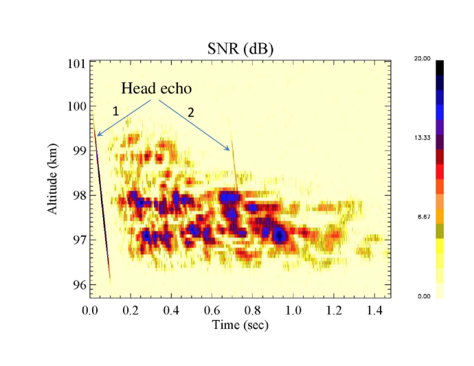
Figure 1: Altitude-time radar image of meteor plasma (JRO, July 12, 2005, 3:43AM LT). The color coding shows the signal-to-noise ratio in dB. The two arrows point to the head echoes of two separate meteoroids. The stronger head echo (1) is followed by a non-specular trail, while the meteoroid with the much weaker head echo (2) produces no detectable trail. The vertical velocity components of both meteoroids were close. The head-echo slope gives the corresponding downward speed about $40$ km/s.

Meteor plasma is usually a few orders of magnitude denser than the ambient ionosphere, especially during a night time. High-power large aperture (HPLA) radars located near the magnetic equator, such as Jicamarca Radio Observatory (JRO) or ALTAIR, often detect signals composed of two distinct parts, the head echo and non-specular (range-spread) trail, as shown in Figure 1. On an altitude-time diagram, the head echo resembles an almost straight line. It forms when a radar beam scatters from a dense plasma that accompanies an ablating meteoroid. The reflected signal has high Doppler shift, showing that the plasma moves at or near the velocity of the meteoroid.

This paper analyzes the structure of short-lived near-meteoroid plasmas that produce radar head echoes. An accurate model of this structure will enable us to better use these measurements to estimate meteoroid characteristics (Bronshten, 1983; Ceplecha et al., 1998). This work has also another motivation. Big meteor fireballs produce strong electromagnetic pulses that result in audible sounds called electrophonics (Bronshten, 1983; Ceplecha et al., 1998; Keay, 1995; Zgrablić et al., 2002; Chakrabarti et al., 2005; Lashkari et al., 2015). Recent ground-based antenna observations during meteor storms have demonstrated that small, optically invisible, meteoroids can also produce detectable electromagnetic pulses (Price and Blum, 2000; Rault, 2010; De et al., 2011; Guha et al., 2012; Obenberger et al., 2014). To understand the physical nature of these pulses and some of their non-trivial spectral features, it is desirable to quantitatively understand the transient electric current system associated with the near-meteoroid plasma. The kinetic theory of this paper should help model this system. It could also predict whether the near-meteoroid plasma can develop plasma instabilities that might be responsible for submillisecond modulations of the observed ELF/VLF pulses (Price and Blum, 2000).

Many previous theoretical studies of meteor plasma were devoted to estimating the parameter $\beta$ that characterizes the meteor ionization efficiency, the number of electrons generated by a meteoroid of a given speed and altitude per unit length (Massey and Sida, 1955; Furman, 1960, 1961, 1964, 1967; Lazarus and Hawkins, 1963; Sida, 1969; Jones, 1997; Bronshten, 1983); see also Ceplecha et al. (1998) and references therein. One of the earliest works that dealt with the spatial structure of the ablated meteoric material is that of Manning (1958) who modelled the initial radius of the collisionless kinetic expansion of a cylindrical trail followed by its regular collisional diffusion. This model was based on simplified assumptions like elastic sphere collisions, random walks leading to Gaussian trails, meteoric ions ablated directly from the meteoroid, etc. The most cited work by Jones (1995) re-examined and developed this approach further using both theory and particle simulations. Jones’s simulations have demonstrated significant deviations of the initial plasma from the Gaussian profile across the plasma trail. The major goal of those earlier studies was to model the 2-D transition from the initial ballistic expansion to the regular collisional diffusion of the cylindrical plasma trail behind the meteoroid. These studies were based on probabilistic averaging and they did not really study the 3-D spatial distribution of the dense plasma that surrounds the fast-moving meteoroid and is responsible for the radar head echo.

The meteor plasma that causes the head echo is distributed within a small near-meteoroid volume whose effective size is of order of the collisional mean free path. This and some other factors lead to strongly non-Maxwellian velocity distributions and require a kinetic description. However, none of the earlier studies have developed a consistent kinetic theory. Recently, Dyrud et al. (2008a, b) made a first attempt of modeling the spatial structure of the near-meteoroid plasma kinetically using particle-in-cell (PIC) simulations. Their modeling generated a plausible qualitative picture of what might be expected but did not provide quantitative characteristics or simple parameter dependences that would allow radar signal modeling and related physical analysis. The more recent paper by Stokan and Campbell-Brown (2015) modeled collisions of ablated particles but, similar to the early studies, it mostly studied the wake formation behind the meteoroid. Our earlier theoretical papers mostly analyzed the slowly diffusing plasma columns related to the non-specular trails (Dimant and Oppenheim, 2006a, b).

This paper develops a kinetic theory of the plasma formed around a fast-descending meteoroid. Based on this theory, in a companion paper, we calculate the 3-D spatial structure of the near-meteoroid plasma density required for interpretation of radar head echoes. Future publications will include a more detailed theoretical analysis, computer simulations, and discussion of implications for real meteors and comparisons with radar observations.

This paper is organized as follows. In section 2 we discuss the physical conditions of the actual meteors in atmosphere and our choice of the relevant theoretical assumptions. In section 3 we formulate the kinetic equation with the appropriate collisional operator, while in section 4 we describe the general approach to its solution. In section 5 we calculate the distribution function of the primary, i.e., ablated meteoric particles that have not yet experienced any collisions with the dense atmosphere. In section 6 we calculate the distribution function of the secondary particles (newly born ions and singly-scattered neutrals). This section describes the kinetics of almost all near-meteoroid ions and is central to the paper. In section 7 we summarize our objectives and findings. Appendix provides some mathematical details related to section 6.

2 Physical conditions and principal theoretical assumptions

In this section, we analyze physical conditions of the meteor plasma formation and justify our theoretical approximations. Readers who are not interested in this justification can proceed directly to section 3.

A fast descending meteoroid creates around itself a strong disturbance which we will call the ‘near-meteoroid sheath.’ It includes several components: (1) the ‘primary,’ mostly neutral, particles ablating from the meteoroid surface and continuing their free ballistic motion until they collide with atmospheric molecules; (2) collisionally scattered and ionized particles of both meteoric and atmospheric materials; (3) free electrons released during the ionizing collisions. This paper develops the kinetics of the heavy particles of components (1) and (2).

Our analytical approach assumes that the kinetic energy of the ablated atoms in the rest frame of the atmosphere greatly exceeds the thermal energy of the ablated atoms and this greatly exceeds the thermal energy of the neutral atmosphere. Hence,

$$T_{\mathrm{A}}\ll T_{\mathrm{M}}\ll\frac{m_{\mathrm{A,M}}U^{2}}{2},$$ (1)

where $T_{\mathrm{A}}$ is the undisturbed atmospheric temperature, $T_{\mathrm{M}}<1\,\mathrm{eV}$ is the characteristic temperature of the ablated meteoric particles (both in the energy units), $m_{\mathrm{A,M}}\sim(30$–$50)\,\mathrm{amu}$ are the corresponding molecular or atomic masses, and $U=|\vec{U}|$ is the meteoroid speed. It also assumes a tiny meteoroid, much smaller than any other scales in the system, such that,

$$r_{\mathrm{M}}\ll\lambda\ll H,L.$$ (2)

where $r_{\mathrm{M}}$ is the average meteoroid radius, $\lambda$ is the characteristic length scale of the near-meteoroid sheath (of order of the collisional mean free path), and $H$ is the scale height of atmosphere, and $L$ is a characteristic length scale of spatial variations along the meteoroid trajectory such as the meteoroid velocity, $-\vec{U}$, temperature, and material composition.

The inequality $r_{\mathrm{M}}\ll\lambda$ precludes small meteoroids from forming shock waves. The inequalities $\lambda\ll H,L$, suggest a simple adiabatic approach when over the characteristic length of the near-meteoroid sheath $\sim\lambda$ at a given altitude $h$, we can treat the atmosphere as a uniform gas with the local density $n_{\mathrm{A}}$ and constant meteoroid parameters. Differential ablation (von Zahn et al., 1999; Vondrak et al., 2008; Janches et al., 2009) and meteoric fragmentation (Kero et al., 2008; Roy et al., 2009; Mathews et al., 2010) might in principle break this gradual adiabatic behavior. However, these processes present no real challenge to our theory.

Additionally, we will assume that the sheath particles collide almost exclusively with the undisturbed neutral atmosphere of a given density and composition, rather than between themselves. For simplicity, we will also assume that the undisturbed neutral atmosphere includes only one atmospheric species with the known density, $n_{\mathrm{A}}(h)$, mean molecular mass, $m_{\mathrm{A}}$, and given velocity-dependent collision frequency. We will also neglect inelastic collisions with the energy losses, $\Delta E_{\mathrm{in}}\lesssim 10$ eV, compared to

$$\frac{m_{\mathrm{A,M}}U^{2}}{2}\approx 140\,\mathrm{eV}\left(\frac{m_{\mathrm{A,M}}}{30\,\mathrm{amu}}\right)\left(\frac{U}{30\,\mathrm{km}/\mathrm{s}}\right)^{2}.$$ (3)

We will initially include $\Delta E_{\mathrm{in}}$ for estimates and future references, but in the rest of our theory we will neglect it.

Our most serious assumption is that between consecutive collisions ions are weakly affected by fields and have almost straight-line ballistic trajectories as do neutral particles. In this paper, we neglect completely the electric and magnetic fields on the ion orbits. This can be justified by considering the electron dynamics. Electrons released during the collisional ionization of neutral particles form the vast majority of free electrons around the descending meteoroid. Their characteristic kinetic energy, $\mathcal{E}_{e}$, is typically below a few electronvolts with the corresponding electron speed given by

$$V_{e}=\sqrt{\frac{2\mathcal{E}_{e}}{m_{e}}}\approx 1.3\times 10^{3}\ \mathrm{km}/\mathrm{s}\left(\frac{\mathcal{E}_{e}}{5\,\mathrm{eV}}\right)^{1/2},$$

where $m_{e}$ is the electron mass. This speed far exceeds the hypersonic meteoroid speed of $U\lesssim 70~{}\mathrm{km/s}$, so that after release from a neutral particle, the electron could travel long distances away from the meteoroid unless it is confined by the geomagnetic field, $\vec{B}$, and an electrostatic field, $\vec{E}=-\nabla\Phi$. At altitudes $\gtrsim 80\ \mathrm{km}$ electrons are highly magnetized with the characteristic Larmor radius given by

$$\rho_{e}\approx 0.3\,\mathrm{m}\left(\frac{\mathcal{E}_{e}}{5\,\mathrm{eV}}\right)^{1/2}\left(\frac{2.5\times 10^{-5}\,\mathrm{T}}{B}\right),$$

where $2.5\times 10^{-5}\,\mathrm{T}$ is the typical value of the magnetic intensity, $B=|\vec{B}|$, at the geomagnetic equator. Such relatively small values of $\rho_{e}$ force the newly born electrons to remain practically attached to the original magnetic field line (in the Earth’s frame), but these electrons still could travel freely along $\vec{B}$. However, as electrons move away from the much slower ions they immediately create a charge separation that builds up for them a retarding electrostatic barrier. The corresponding ambipolar electric field is the main force that distorts the orbits of free ions.

We can estimate this potential barrier by assuming a Maxwellian electron velocity distribution with the uniform effective temperature, $T_{e}$, in the few-electronvolts range (e.g., $T_{e}\sim 3\ \mathrm{eV}$). This velocity distribution translates to the Boltzmann distribution of the electron density, $n_{e}(\vec{r}_{1})/n_{e}(\vec{r}_{2})\simeq n_{0}\exp(e\Delta\Phi/T_{e})$, where $n_{e}(\vec{r}_{1,2})$ are the electron densities in two different locations and $\Delta\Phi=\Phi(\vec{r}_{1})-\Phi(\vec{r}_{2})$ is the corresponding potential difference. The built-up ambipolar electrostatic field, $\vec{E}=-\nabla\Phi$, retards electrons but accelerates ions. Assuming the quasi-neutrality, $n_{e}\simeq n_{i}$, we can easily estimate the potential difference between a given location inside the dense electron sheath and its edge. Loosely defining this edge by setting the meteor-plasma density to be of order of the background ionospheric density, $n_{\mathrm{ionos}}$, to a logarithmic accuracy we obtain

$$e\Delta\Phi\simeq T_{e}\ln\frac{n_{i}}{n_{\mathrm{ionos}}}.$$ (4)

Assuming the meteor plasma to be a few orders of magnitude denser than the background ionosphere, we obtain that $e\Delta\Phi\lesssim 30~{}$eV. Since this $e\Delta\Phi$ is noticeably smaller than the characteristic ion kinetic energy $\mathcal{E}_{i}\sim m_{i}U^{2}/2$ given by equation (3) then to a zero-order approximation we can neglect the $\vec{E}$-effect on ions.

There is an additional field that can affect the ion trajectories. If the descending meteoroid with the velocity $-\vec{U}$ crosses the magnetic field $\vec{B}$ then in its frame $\vec{B}$ induces the dynamo electric field $\vec{E}=\vec{U}\times\vec{B}$. At the altitudes of $80\ \mathrm{km}\lesssim h<120\$km, ions are almost unmagnetized due to frequent collisions with the atmosphere, $\Omega_{i}\ll\nu_{i}$, where $\Omega_{i}\$is the ion gyrofrequency. The characteristic size of the near-meteoroid plasma sheath, $\lambda$, is of order of the ion mean free path, $\lambda\lesssim U/\nu_{i}$. Then the corresponding potential difference across the sheath is $e\Delta\Phi\sim eE\lambda\lesssim\left(\Omega_{i}/\nu_{i}\right)m_{i}U^{2}\ll\mathcal{E}_{i}$. Thus the induced electric field is also relatively weak.

In this paper we neglect $\vec{E}$ completely and assume the sheath electrons to roughly follow the Boltzmann distribution with quasi-neutrality. This closes the kinetic description of ions and allows ignoring the geomagnetic field, $\vec{B}$. This in turn leads to the axial symmetry around the straight-line meteoroid trajectory. We will improve our theoretical model in future by using computer simulations.

To conclude this section, we note that most ions should originate from the ablated meteoric particles due to their lower ionization potential, but a certain fraction of the atmosphere can also be collisionally ionized. Additionally, particles ablating from the meteoroid surface should be mostly neutral, but a small fraction of them could be ionized. The general kinetic framework of this paper encompasses all these possibilities.

3 Formulation of the kinetic problem

The description of the near-meteoroid sheath around a descending meteoroid requires a kinetic theory for two main reasons: (1) the characteristic length scales of the near-meteoroid sheath are of order of the collisional mean free paths and (2) the two colliding velocity distributions – the ablative flow from the meteoroid surface and the impinging neutral atmosphere – are shifted with respect to each other by a huge hypersonic velocity, $\vec{U}$. According to (1), the near-meteoroid sheath forms a marginally collisional structure. It includes mostly the ‘primary’ (ablated) particles that travel freely before suffering their first collision and the ‘secondary’ particles, i.e., particles scattered or ionized only once since the original ablation. According to (2), after one or two collisions the two impinging flows redistribute their huge energy difference only partially, so that the velocity distributions of the sheath particles become neither isotropic nor Maxwellian. No fluid model can adequately describe such distributions.

The primary interest of this paper lies in the near-meteoroid plasma, but because we neglect field effects, as described in section 2, the kinetic framework of this paper does not distinguish between the near-meteoroid plasma and the neutral sheath. Between consecutive collisions, all heavy meteoric particles move over straight-line ballistic trajectories, although the ion-neutral collisions differ from the neutral-neutral collisions. We presume given expressions for each collisional cross-section. Apart from these specific expressions, the sheath ions and neutral particles are described by the same general equations.

Now we consider a group of the sheath particles with the given material and charge state. This group is characterized by the velocity distribution $f(\vec{V},\vec{r})$, so that the corresponding particle and flux densities are given by $n=\int f(\vec{V},\vec{r})d^{3}V$ and $\vec{\Gamma}=\int f(\vec{V},\vec{r})\vec{V}d^{3}V$, respectively. We do not index variables with the explicit group identifiers because the general equations written below are applicable to any group. We will develop our kinetic theory based on the collisional kinetic equation derived in Appendix A. This equation generalizes the standard kinetic equation with the Boltzmann collision operator (Huang, 1987; Lifshitz and Pitaevskii, 1981) to inelastic collisions, albeit in a simplified form, as described below. Under stationary conditions in the meteoroid frame of reference, the initial kinetic equation with binary collisions can be written as

$$(\vec{V}\cdot\nabla)f=-\nu(\vec{V})f+\hat{S}_{\mathrm{gain}}[f^{\prime}].$$ (5)

The left-hand side (LHS) of equation (5) describes the ballistic motion of the particles between the consecutive collisions.

The right-hand side (RHS) of equation (5) describes the binary collision operator. The first term describes the collisional “loss” from a given elementary volume of the 6D phase space (Lifshitz and Pitaevskii, 1981), $d^{3}Vd^{3}V_{\beta}$, where $\vec{V}$ is the 3D vector of the meteoric particles described by the given distribution function $f$, while $\vec{V}_{\beta}$ is the velocity of the colliding partners (atmospheric particles) described by $f_{\beta}$, and $\nu(\vec{V})$ is the velocity-dependent kinetic collision frequency,

$$\nu(\vec{V})=\sum_{\beta}\int f_{\beta}G\left(u,\Lambda\right)ud^{3}V_{\beta}d\Omega_{\mathrm{s}}\approx 2\pi n_{\mathrm{A}}\int_{-1}^{1}uG\left(u,\Lambda\right)d\Lambda,$$ (6)

where $u=|\vec{u}|$ is the relative speed of the two colliding particles and $\Lambda$ is the cosine of the corresponding scatter angle, as will be explained below. The second term in the RHS of equation (5) is the “gain” component of the collision operator. It is written as an integral operator $\hat{S}_{\mathrm{gain}}$ acting on $f^{\prime}$, and expresses the collisional kinetic arrival at $d^{3}Vd^{3}V_{\beta}$ from other elementary volumes, $d^{3}V^{\prime}d^{3}V_{\beta}^{\prime}$.

$$\hat{S}_{\mathrm{gain}}[f^{\prime}]=\sum_{\beta}mm_{\beta}\left(m+m_{\beta}\right)^{2}\int f^{\prime}f_{\beta}^{\prime}\left(\frac{u^{\prime}}{u}\right)G\left(u^{\prime},\Lambda^{\prime}\right)d^{3}V_{\beta}d^{3}V_{\beta}^{\prime}d^{3}V^{\prime}$$

$$\times\delta\left(m\vec{V}^{\prime}+m_{\beta}\vec{V}_{\beta}^{\prime}-m\vec{V}-m_{\beta}\vec{V}_{\beta}\right)\delta\left(E^{\prime}+E_{\beta}^{\prime}-E-E_{\beta}-\Delta E_{\mathrm{in}}\right)$$ (7a)

$$=\sum_{\beta}\int f^{\prime}\ \frac{\left(u^{\prime}\right)^{2}}{u}\ G\left(u^{\prime},\Lambda\right)f_{\beta}^{\prime}d^{3}V_{\beta}^{\prime}d\Omega_{\mathrm{s}},$$ (7b)

where $f^{\prime}\equiv f(\vec{V}^{\prime})$, $f_{\beta}^{\prime}\equiv f_{\beta}(\vec{V}_{\beta}^{\prime})$, and the single integral sign denotes integrations over all three 3D volumes of $\vec{V}_{\beta}$, $\vec{V}_{\beta}^{\prime}$, and $\vec{V}^{\prime}$. Equation (7) generalizes the corresponding part of the Boltzmann collision operator (Huang, 1987; Lifshitz and Pitaevskii, 1981; Shkarofsky et al., 1966) to non-elastic collisions. Each of its components will be defined and explained in the next few pages.

In the general case, the summation over $\beta$ should include all collision partners described by $f_{\beta}$ or $f_{\beta}^{\prime}$, even the given particles described by $f$. However, since we neglect collisions between meteoric particles, the subscript $\beta$ in equations (5)–(7) pertains exclusively to the atmospheric particles. This makes integro-differential equation (5) linear with respect to $f$.

The left inequality of equation (1) allows approximating atmospheric particles in the meteoroid frame by a monoenergetic beam with the $\delta$-function velocity distribution,

$$f_{\mathrm{A}}\approx n_{\mathrm{A}}\delta(\vec{V}-\vec{U}).$$ (8)

The last, approximate, equality in equation (6) uses equation (8) where $n_{\mathrm{A}}(h(t))$ is the given local atmospheric density at an altitude $h$ crossed by the meteoroid at a given moment $t$.

The linear character of kinetic equation (5) allows one to treat each group of colliding particles separately with separate terms like in equations (6) and (7), each responsible for a given kind of collision processes. These processes should include all elastic and inelastic collisions with the atmosphere, e.g., collisional ionization of meteoric atoms or elastic scattering of the corresponding ions. The ionization part of the ‘loss’ term for neutrals becomes the corresponding ‘gain’ term for the newly born ions.

In equation (7), $G\left(u^{\prime},\Lambda\right)=d\sigma/d\Omega_{\mathrm{s}}$ is the differential cross-section taken as a function of frame-invariant variables, such as $u^{\prime}=|\vec{u}^{\prime}|$ and

$$\Lambda\equiv\cos\Theta_{\mathrm{s}}=\frac{\vec{u}\cdot\vec{u}^{\prime}}{uu^{\prime}}.$$ (9)

Here $\vec{u}^{\prime}=\vec{V}^{\prime}-\vec{V}_{\beta}^{\prime}$ and $\vec{u}=\vec{V}-\vec{V}_{\beta}$ are the relative velocities of the two colliding particles before and after the collision, respectively; in equation (7) all primes denote particle velocities before the collision, $\vec{V}^{\prime},\vec{V}_{\beta}^{\prime}\rightarrow\vec{V},\vec{V}_{\beta}$. The scattering angle $\Theta_{\mathrm{s}}$ in equation (9) is defined as the polar angle of $\vec{u}^{\prime}$ in the spherical system with the major axis directed along $\vec{u}$. In the absence of strong external fields, the colliding molecules are on average unpolarized, hence we assume $G$ to be independent of the second, i.e., axial, scattering angle, $\Phi_{\mathrm{s}}$. In the general case of inelastic collisions with the collisional loss of the total kinetic energy $\Delta E_{\mathrm{in}}$, $u^{\prime}$ and $u$ are related as

$$u^{\prime}=\left(u^{2}+\frac{2\Delta E_{\mathrm{in}}}{M}\right)^{1/2}.$$ (10)

where $M=mm_{\beta}/(m+m_{\beta})$ is the reduced mass of the two colliding particles.

Equation (7) shows two equivalent forms of $\hat{S}_{\mathrm{gain}}[f^{\prime}]$. Equation (7a) gives a probabilistic form that precedes the conventional Boltzmann form (Lifshitz and Pitaevskii, 1981) (in the strict sense, the latter is only applicable to elastic collisions). We will employ the form (7a) because it allows for a more accurate account of inelastic collisions and, more importantly, this form will enable us to obtain an explicit analytic solution for the velocity distribution of the secondary particles (see section 6). Equation (7b) allows us to verify conservation of the total number of colliding particles,

$$\int\hat{S}_{\mathrm{gain}}[f^{\prime}]d^{3}V^{\prime}=\int\nu(\vec{V})fd^{3}V.$$ (11)

According to equation (5), this leads to the stationary continuity equation:

$$\nabla\cdot\vec{J}=0.$$ (12)

Equations (11) and (12) directly apply to particle scattering without ionization. If inelastic collisions involve ionization, i.e., a partial conversion of one group (neutral particles) to another group (ions) then equations (11) and (12) can be easily extended.

In equation (7a), the $\delta$-functions in the integrand express the conservation of the total particle energy (there $E\equiv mV^{2}/2$ and $E_{\beta}\equiv m_{\beta}V_{\beta}^{2}/2$) and momentum of all colliding particles during one collision act. In the center-of-mass frame, $m\vec{V}+m_{\beta}\vec{V}_{\beta}=m\vec{V}^{\prime}+m_{\beta}\vec{V}_{\beta}^{\prime}=0$, we easily express the individual particle velocities in terms of $\vec{u}$, $\vec{u}^{\prime}$ as

$$\vec{V} =\frac{m_{\beta}\vec{u}}{m+m_{\beta}},\qquad\vec{V}_{\beta}=-\ \frac{m\vec{u}}{m+m_{\beta}},$$

$$\vec{V}^{\prime} =\frac{m_{\beta}\vec{u}^{\prime}}{m+m_{\beta}},\qquad\vec{V}_{\beta}^{\prime}=-\ \frac{m\vec{u}^{\prime}}{m+m_{\beta}},$$ (13)

so that

$$E+E_{\beta}=\frac{Mu^{2}}{2},\qquad E^{\prime}+E_{\beta}^{\prime}=\frac{M(u^{\prime})^{2}}{2}.$$ (14)

Equation (13) yields the relation $d^{3}V^{\prime}=[m/(m+m_{\beta})]^{3}\left(u^{\prime}\right)^{2}du^{\prime}d\Omega_{\mathrm{s}}$, which helps check the equivalence of the two forms of $\hat{S}_{\mathrm{gain}}[f^{\prime}]$. Equation (14), along with the energy conservation, yields equation (10).

Strictly speaking, the integrals in (5) should also include summations over discrete energies of the internal degrees of freedom (for inelastic scattering) and continuous integrations over the kinetic energies of the released free electron (for ionizing collisions). For simplicity, however, we consider only one average discrete energy loss, $\Delta E_{\mathrm{in}}$. For example, for ionizing collisions, we set $\Delta E_{\mathrm{in}}=I+\left\langle E_{e}\right\rangle$, where $I$ is the ionization potential potential and $\left\langle E_{e}\right\rangle$ is the average kinetic energy of the released electrons. For the present treatment, the imposed inaccuracy is not important because the corresponding energy losses (usually $<10~{}$eV) are small compared to the typical kinetic energies of the colliding heavy particles, as discussed in section 2. When obtaining analytic solutions of the kinetic equation, we will neglect $\Delta E_{\mathrm{in}}$, making inelastic processes essentially equivalent to the elastic ones. This is even more so for the total momentum changes associated with the release of a free electron after an ionizing collision. We have not even included such momentum changes, $P_{\mathrm{in}}$, in the argument of the corresponding $\delta$-function because the relative momentum changes are much smaller than the corresponding relative energy changes, $P_{\mathrm{in}}/(mV)\lesssim\left(m_{e}/m\right)\left[\Delta E_{\mathrm{in}}/(mV^{2}/2)\right]\ll\Delta E_{\mathrm{in}}/(mV^{2}/2)$.

Collisions of meteor particles with atmospheric molecules have a twofold effect: they scatter and ionize the meteoroid particles, and at the same time they scatter the atmospheric molecules and can even ionize the latter, albeit with a smaller efficiency. On a par with the meteoric particles, the scattered atmospheric molecules and the corresponding molecular ions could also be included as separate kinetic groups with the corresponding velocity distributions. However, the relative number of scattered atmospheric molecules is so low compared to the total amount of undisturbed atmospheric particles that they will be of no interest to us. By contrast, the collisionally born molecular ions of atmospheric origin could in principle make a noticeable contribution to the near-meteoroid plasma.

Before proceeding with the solution of equation (5), we note the following. If calculated classically, $\nu$ defined by equation (6) diverges, unless the interaction force between the two colliding particles becomes exactly zero when the interparticle distance $R$ exceeds a certain finite value (as in hard-sphere collisions). The ‘gain’ term $\hat{S}_{\mathrm{gain}}[f^{\prime}]$ has the same problem. The diverging long-distance part of $G(u,\Lambda)$ corresponds to scattering through small angles, $\Theta_{s}\rightarrow 0$. In terms of equation (6) and (7), this means a non-integrable singularity of $G(u,\Lambda)$ when approaching the upper integration limit of $\Lambda=1$. In Coulomb collisions with the interaction potential $V_{\mathrm{int}}\propto 1/R$, the long-distance scattering through small angles dominates. However, if at least one of the interacting particles is neutral then the asymptotic long-distance interaction becomes $V_{\mathrm{int}}\propto 1/R^{n}$ with $n\geq 4$ (McDaniel, 1989, 1993; Kaganovich et al., 2006). The corresponding scattering through small angles is no longer dominant and plays insignificant role in collisional changes of the particle momenta. Nonetheless, even exponentially decreasing interactions would formally lead to the divergent total cross-section. More accurate quantum-mechanical calculations yield convergent $\nu$, but they can lead to operating with physically meaningless long distances.

We will avoid the integral divergence by noticing the following. The formally dominant contribution of small-angle scattering means that $\hat{S}_{\mathrm{gain}}[f^{\prime}]$ and $\nu(\vec{V})f$ in equation (5) become indefinitely large, but they must almost perfectly balance each other to provide a finite difference. In collisions that involve at least one neutral particle, small-angle scattering creates so minuscule momentum changes that they result in no perceptible phase-space redistributions of particles. Then by slightly regrouping the particles we can renormalize $\hat{S}_{\mathrm{gain}}[f^{\prime}]$ and $\nu(\vec{V})f$ in such a way that would eliminate the closely balancing large parts. In order to avoid a tedious renormalization procedure, we will merely assume the given cross-section $G(u,\Lambda)$ to be a regular function of $\Lambda$. This assumption is equivalent to cutting off the non-essential asymptotic parts of long-distance interactions, so that ion-neutral and neutral-neutral collisions become in a sense similar to hard-sphere collisions.

4 Outline of the general kinetic solution

To solve equation (5), we will use the kinetic approach developed previously for Compton scattering of $\gamma$-quanta propagating through dense air (Dimant et al., 2012). We will represent the total velocity distribution, $f$, as a series of partial distributions,

$$f=f^{\left(1\right)}+f^{\left(2\right)}+f^{(3)}+\ldots,$$ (15)

where the superscript denotes the total number of collisions the corresponding particles experienced since their original ablation plus one. For example, $f^{\left(1\right)}$ describes the sub-group of primary particles ablated from the meteoroid and freely propagating before they encounter their first collisions. The function $f^{\left(2\right)}$ describes a sub-group of secondary particles that experienced exactly one collision since their original ablation. This sub-group includes neutral particles scattered once and newly-born ions originated during an ionizing collision of a primary particle with the atmosphere. The function $f^{(3)}$ describes a sub-group of tertiary particles that experienced exactly two collisions since the original ablation, and so forth.

The linear character of kinetic equation (5) allows one to obtain a closed differential equation for the partial function $f^{(j)}$ in terms of $f^{(j-1)}$,

$$(\vec{V}\cdot\nabla)f^{(j)}+\nu^{(j)}(u)f^{(j)}=\hat{S}_{\mathrm{gain}}[f^{(j-1)}],$$ (16)

where the superscripts describe the corresponding particle sub-groups and $\nu^{(j)}(u)$ is given by equation (6) for the corresponding sub-group. Particle conservation requires that the collision terms satisfy the relationship

$$\int\hat{S}_{\mathrm{gain}}[f^{(j-1)}]d^{3}V=\int\nu^{(j)}(u)f^{(j)}d^{3}V,$$ (17)

similar to (11). Equation (17) is useful for checking the solutions.

The only preferred direction in the meteoroid frame is the velocity of the impinging atmospheric beam, $\vec{U}$. We will represent $\vec{U}$ vertically directed, as in Figure 2.

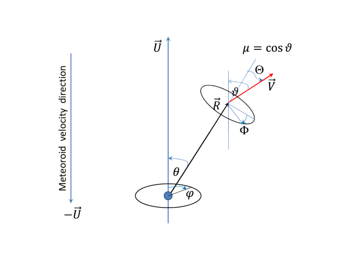
Figure 2: Nomenclature of spatial coordinates and velocity variables. The spatial variables $R=|\vec{R}|$, $\theta$, $\varphi$ denote the radius and two angles of the spherical coordinate system with the origin at the meteoroid center and the major axis anti-parallel to the meteoroid velocity shown on the left. All other variables pertain to the particle velocity space: $V=|\vec{V}|$ is the particle speed, $\vartheta$ is the polar angle of $\vec{V}$ with respect to the local axis parallel to $\vec{U}$, $\Phi$ is the axial angle measured from the common $\vec{U}$-$\vec{R}$ plane; $\Theta$ is the polar angle of $\vec{V}$ with respect to the local radial distance $\vec{R}$.

In real space, we will use the spherical coordinate system characterized by the radial distance $R$ measured from the meteoroid center, the polar angle $\theta$ with respect to the major axis aligned with $\vec{U}$, and the corresponding axial angle $\varphi$, as shown in Figure 2.

Equation (16) with the given RHS can be solved by characteristics. However, in the velocity space we should use variables that remain invariant along the ballistic particle trajectories and at the same time employ the assumed symmetry. We will use variables $V$, $R_{0}$ and $\Phi$, where $V$ is the particle speed, $R_{0}=R\sin\Theta$, while $\Theta$ and $\Phi$ are respectively the polar and axial angles corresponding to the local spherical system in the velocity space with the major axis aligned with $\vec{R}$. Here $\vec{R}$ is the spatial radius-vector measured from the meteoroid center. The variable $R_{0}$ is the minimum distance between the straight-line trajectory of a particle and the meteoroid center, as shown in Figure 3. This variable can also be interpreted as a renormalized absolute value of the particle angular momentum.

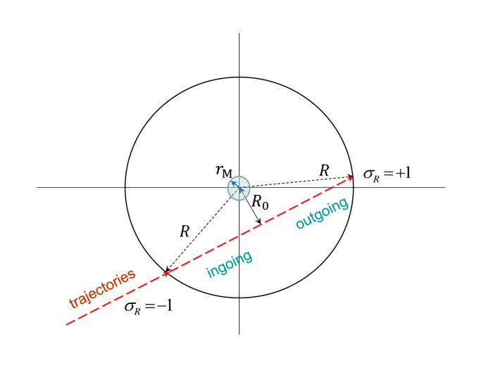
Figure 3: A particle trajectory crossing a sphere of a given radial distance $R$ from the meteoroid center. Here $\varepsilon$ is the meteoroid radius and $R_{0}$ is the minimum distance from the meteoroid center to the trajectory. When an incoming particle ($dr/dt<0$, $\sigma_{R}=-1$) crosses $R_{0}$ it becomes outgoing ($dr/dt>0$, $\sigma_{R}=+1$).

For the primary particles, $j=1$, the RHS of equation (16) is zero, so that the solution for $f^{\left(1\right)}$ is determined only by the boundary conditions on the meteoroid surface and the collisional losses described by $\nu^{(1)}(u)$. For arbitrary $j>1$, the solutions for $f^{\left(j\right)}$ can be obtained recursively, starting from $f^{\left(1\right)}$. The problem is, however, that $\hat{S}_{\mathrm{gain}}[f^{(j-1)}]$ defined by equation (7a) involves multiple integrations, so that the mathematical complexity of finding $f^{\left(j\right)}$ increases dramatically with each following $j$.

Fortunately, the physics of plasma formed around a fast moving meteoroid allows cutting the infinite chain of equation (16) at a specific sub-group with $j=k\geq 2$. The rest of the particles can be included in $f^{\left(k\right)}$ by dropping the second (loss) term in the LHS of equation (16), $\nu^{(j)}f^{(j)}.$ This will automatically provide the particle conservation. Dropping $\nu^{(j)}f^{(j)}$ will also simplify the solution. The downside of including $f^{\left(j\right)}$ with $j>k$ to $f^{\left(k\right)}$ is that the scattered ions with $j>k$ will appear closer to the meteor plasma forefront than they actually are. However, this error will become noticeable only at large distances from the meteoroid, $R\gtrsim\lambda^{\left(k\right)}\gg\lambda^{\left(1\right)}$, where this plasma is mostly inconsequential for the radar head echo.

Indeed, in the meteoroid frame, particles forming $f^{\left(1\right)}$ collide with atmospheric particles that have a huge velocity, $\vec{V}\approx\vec{U}$. As a result, the secondary particles described by $f^{(2)}$ have velocities oriented such that their projection onto the $\vec{U}$-line is almost exclusively in the $\vec{U}$-direction. As $j$ increases further, the core of the corresponding velocity distribution in the meteoroid frame shifts closer to $\vec{U}$. In the atmospheric frame, this means that multiply scattered particles will gradually slow and cool down with the core of the corresponding particle population in the real space lagging behind the fast-descending meteoroid and forming the extended trail. Thus the near-meteoroid sheath is mostly formed by particles with the lowest $j=1,2$, although a small fraction of each population remains in every location. Figure 4 shows schematically such spatial distribution. The distributions $f^{(1,2)}$ should dominate at the forefront of the near-meteoroid sheath, but behind the meteoroid there is no clear interface between the near-meteoroid sheath and extended trail. For our purposes, however, this is unimportant because head-echo radar scattering is determined mostly by the frontal and side edges of the near-meteoroid plasma and less so by the elongated trail behind it. Notice that as described below the characteristic length scale of particle populations with $n\geq 2$ is much larger than that of the primary particles, $\lambda^{(n)}\gg\lambda^{(1)}$.

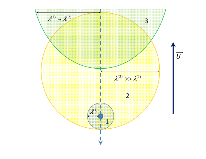
Figure 4: A cartoon of core spatial distributions of the primary (1), secondary (2), and tertiary (3) particles in the meteoroid frame of reference. The core distributions of the higher-order particle sub-groups are shifted farther away from the meteoroid in the direction of $\vec{U}$ (i.e., opposite to the meteoroid velocity). The spherically symmetric core distribution of the primary particles (with the effective radius $\sim\lambda^{(1)}$) occupies a much smaller volume than the core distributions of all other sub-groups. Primary particles are almost entirely neutral, while all other groups include scattered neutrals and ions.

In this paper, we restrict our kinetic theory to the two lowest-order functions $f^{(1,2)}$ that describe the primary and secondary particles that include all higher-order local sub-groups in $f^{(2)}$ through dropping in equation (16) the $\nu^{(2)}f^{(2)}$ term. This approximation will describe the spatial and velocity distribution of all near-meteoroid ions with sufficient accuracy.

5 Velocity distribution of the primary particles

If we neglect direct sputtering of the meteoroid by the impinging atmospheric flow then the velocity distribution of particles ablating from the meteoroid is fully determined by its structure, material composition, and temperature. Since we assume a spherical meteoroid with the radius $r_{\mathrm{M}}$ and uniform temperature $T_{\mathrm{M}}$, the spatial distribution of the primary particles will also be spherically symmetric. The ablated particles initially keep their thermal equilibrium, so that on the meteoroid surface, $R=r_{\mathrm{M}}$, they obey a Maxwellian distribution with the temperature $T_{\mathrm{M}}$. Since we can linearly combine many sources of the ablating particles, we consider one species with the mass $M_{\mathrm{met}}$ and given density $n_{0}$,

$$\left.f^{\left(1\right)}\right|_{R=r_{\mathrm{M}}}=F_{0}\left(V\right)\mathrm{H}\left(\cos\Theta\right),\qquad F_{0}\left(V\right)=\frac{2n_{0}}{\left(2\pi\right)^{3/2}V_{T}^{3}}\mathrm{\ }\exp\left(-\ \frac{V^{2}}{2V_{T}^{2}}\right).$$ (18)

Here $V_{T}=(T_{\mathrm{M}}/M_{\mathrm{met}})^{1/2}$ is the thermal velocity of the ablating gas, $\Theta$ is the polar angle in the velocity space measured from the local radius-vector $\vec{R}$ on the meteoroid surface, and $\mathrm{H}\left(x\right)$ is the Heaviside step-function ($\mathrm{H}\left(x\right)=1$ if $x\geq 0$ and $\mathrm{H}\left(x\right)=0$ otherwise). This step-function expresses the fact that ablating particles leaving the meteoroid can move only outward from the its surface. The corresponding radial flux density near the meteoroid surface is $(J_{R})_{0}=\int\left.f^{\left(1\right)}\right|_{R=r_{\mathrm{M}}}\left(V\cos\Theta\right)d^{3}V=\sqrt{2/\pi}\ n_{0}V_{T}\approx 0.8n_{0}V_{T}$. The parameters $n_{0}$, or $(J_{R})_{0}$, and $T_{\mathrm{M}}$ can be taken from various ablation models, such as CAMOD (Vondrak et al., 2008) and others (Furman, 1960, 1961; Lebedinets and Shushkova, 1970; Lebedinets et al., 1973; Sorasio et al., 2001; Mendis et al., 2005; Dyrud et al., 2005; Campbell-Brown and Close, 2007; Berezhnoy and Borovička, 2010).

At arbitrary distances from the meteoroid center, $R$, the solution for $f^{\left(1\right)}$ can be obtained separately in two overlapped regions: the closer distances $r_{\mathrm{M}}\leq R\ll\lambda^{\left(1\right)}$, where the mean free path for the primary particles, $\lambda^{\left(1\right)}$, is defined by equation (20), and the farther distances, $R\gg r_{\mathrm{M}}$, that include $R\gtrsim\lambda^{\left(1\right)}$. In the former region, the primary particles experience essentially no collisions so that $f^{\left(1\right)}$ is given by equation (18), where the local variable $\Theta$ should be expressed in terms of the invariant variable $R_{0}=R\sin\Theta$. At farther distances, $f^{\left(1\right)}$ starts experiencing collisional losses, but the particles propagate mostly along the local radius-vector $\vec{R}$. As a result, we have to solve equation (16) without the RHS, $(\vec{V}\cdot\nabla)f^{\left(1\right)}+\nu^{\left(1\right)}(u)f^{\left(1\right)}=0$ with $\vec{V}\cdot\nabla\approx V(\partial/\partial R)$. After finding the corresponding solution, matching the two expressions in the overlap, $r_{\mathrm{M}}\ll R\ll\lambda^{\left(1\right)}$, and expressing the invariant variable $R_{0}$ back in terms of the local variable $\Theta$ for the given location $\vec{R}$, we obtain

$$f^{\left(1\right)}\approx\frac{2n_{0}}{\left(2\pi\right)^{3/2}V_{T}^{3}}\ \mathrm{H}\left(\cos\Theta-\sqrt{1-\frac{r_{\mathrm{M}}^{2}}{R^{2}}}\right)\exp\left(-\ \frac{V^{2}}{2V_{T}^{2}}-\frac{R}{\lambda^{\left(1\right)}}\right),$$ (19)

where the mean free path for the primary particles, $\lambda^{\left(1\right)}$, is given by

$$\lambda^{\left(1\right)}(V)=\frac{V}{\nu^{\left(1\right)}},\qquad\nu^{\left(1\right)}\approx 2\pi n_{\mathrm{A}}U\int_{-1}^{1}G\left(U,\Lambda\right)d\Lambda.$$ (20)

Here we have taken into account the fact that $V\sim V_{T}\ll U$, so that $u\approx U$. Equation (20) shows that the collision frequency $\nu^{\left(1\right)}$ is approximately constant and $\lambda^{\left(1\right)}\propto V$, i.e., faster primary particles move farther away from the meteoroid before being collisionally scattered or ionized. Since $V\ll U$, the mean free path of the primary particles, $\lambda^{\left(1\right)}(V)$, is much shorter than the mean free paths for all other sub-groups with $V\sim U$, but is still many orders of magnitude longer than the meteoroid radius, $r_{\mathrm{M}}$.

6 Velocity distribution of the secondary particles

The group of secondary particles, $f^{\left(2\right)}$, includes most ions of the near-meteoroid plasma. Calculation of $f^{\left(2\right)}$ is more complicated than $f^{\left(1\right)}$ and is the central topic of this paper.

After cutting the infinite chain described by equation (16) at $k=2$ and dropping the corresponding loss term, the closed kinetic equation for $f^{\left(2\right)}$ becomes

$$(\vec{V}\cdot\nabla)f^{(2)}=\hat{S}_{\mathrm{gain}}[f^{(1)}].$$ (21)

In order to obtain the explicit analytical expression for $f^{\left(2\right)}$, we have to calculate $\hat{S}_{\mathrm{gain}}[f^{\left(1\right)}]$ and then integrate it over the characteristics of equation (21). Before proceeding, we will first discuss individual collisions of primary particles with an almost monoenergetic beam of atmospheric molecules. This analysis will suggest a relevant approximation of $\hat{S}_{\mathrm{gain}}[f^{(1)}]$ that will eventually lead us to a proper analytic solution for $f^{\left(2\right)}$.

6.1 Collisions of individual primary particles with the atmosphere

Consider an individual collision of a primary meteoric particle with a cold atmospheric particle. Before the collision, the meteoric-particle velocity in the meteoroid frame was $\vec{V}^{\prime}$, while the atmospheric molecule velocity in the same frame was $\vec{V}_{\beta}^{\prime}=\vec{U}$. Given the meteoric particle velocity after the collision, $\vec{V}$, and applying the momentum conservation, we obtain the atmospheric-molecule velocity immediately after the collision:

$$\vec{V}_{\beta}=\frac{m}{m_{\beta}}(\vec{V}^{\prime}-\vec{q}),\qquad\vec{q}\equiv\vec{V}-\frac{m_{\beta}\vec{U}}{m}$$ (22)

(the reason for introducing $\vec{q}$ will become clear in section 6.2). From this point on, we will neglect inelastic losses of energy, so that $u=u^{\prime}$. Rewriting the latter as $u^{2}-\left(u^{\prime}\right)^{2}=\left(\vec{u}+\vec{u}^{\prime}\right)\cdot\left(\vec{u}-\vec{u}^{\prime}\right)=0$ with $\vec{u}\equiv\vec{V}-\vec{V}_{\beta}$, $\vec{u}^{\prime}\equiv\vec{V}^{\prime}-\vec{V}_{\beta}^{\prime}=\vec{V}^{\prime}-\vec{U}$, and using equation (22) for $\vec{V}_{\beta}$, we obtain

$$\left[\left(1+\frac{m}{m_{\beta}}\right)\vec{V}+\left(1-\frac{m}{m_{\beta}}\right)\vec{V}^{\prime}-2\vec{U}\right]\cdot(\vec{V}-\vec{V}^{\prime})=0.$$ (23)

As discussed above, before the collision a typical primary-particle speed, $V^{\prime}\sim(2T_{\mathsf{M}}/m_{\mathrm{M}})^{1/2}$, was small compared to $U$. Then to the zeroth-order accuracy corresponding to $\vec{V}^{\prime}\rightarrow 0$ equation (23) yields

$$V\approx V_{Q}(\mu)\equiv\frac{2\mu m_{\beta}U}{m+m_{\beta}},$$ (24)

where $\mu\equiv\cos\vartheta=\vec{V}\cdot\vec{U}/(VU)$ and $\vartheta$ is the polar angle of the particle velocity with respect to the $\vec{U}$ direction, as shown in Figure 2. According to equation (24), the $\vec{V}^{\prime}\rightarrow 0$ approximation allows only positive values of $\mu$: $0\leq\mu\leq 1$ ($\pi/2\geq\vartheta\geq 0$). Under this approximation, the relative velocities of the colliding particles and the cosine of the corresponding scattering angle, $\Lambda=\cos\Theta_{\mathrm{s}}$, are given by

$$\vec{u}^{\prime} \approx-\vec{U},\qquad\vec{u}\approx\left(1+\frac{m}{m_{\beta}}\right)\vec{V}-\vec{U},$$

$$u^{\prime} =u\approx U,\qquad\Lambda=\frac{\vec{u}^{\prime}\cdot\vec{u}}{u^{2}}\approx 1-2\mu^{2}.$$ (25)

Unlike $\mu$, the scattering parameter $\Lambda$ spans the entire domain between $1$ and $-1$ ($0\leq\Theta_{\mathrm{s}}\leq\pi$).

The speed of the secondary particles, $V$, reaches its maximum value, $V_{\max}\approx 2m_{\beta}U/\left(m+m_{\beta}\right)$, for $\mu=1$ corresponding to the backward scatter, $\Theta_{\mathrm{s}}=\pi$ ($\Lambda=-1$). In the opposite limit of small-angle scattering, $\Theta_{\mathrm{s}}\rightarrow 0$ ($\Lambda\rightarrow 1$), equations (24) and (25) yield $\mu,V\rightarrow 0$. In this limit, however, the approximation of $\vec{V}^{\prime}\rightarrow 0$ is inaccurate. In reality, particles scattered through small angles acquire, after a collision, not a zero but a small speed, $V\sim V^{\prime}\ll U$, with arbitrary $\vartheta$. Equation (23) accounts for all cases, but fully neglecting $\vec{V}^{\prime}$ does not work if $\Theta_{\mathrm{s}}\lesssim[(m+m_{\beta})/(2m_{\beta})]V^{\prime}/U$ when $V$ and $V^{\prime}$ become comparable. However, under conditions when slow primary particles collide with extremely fast-moving atmospheric particles, the small-angle collisions retaining the slow speed of the primary particles, $V\sim V^{\prime}\ll U$, are so rare that they make no tangible contribution to the total velocity distribution of the secondary particles. This allows one to neglect small-angle scattering and employ equations (24)–(25) everywhere, regardless of the inaccuracy near $\Lambda=1$ ($\mu=0$).

The fact that the zero-order approximation with respect to $V^{\prime}/U\ll 1$ yields the one-to-one correspondence between $V$ and $\mu$ given by equation (24) leads to the following important consequence. The 3-D velocity distribution of the secondary particles is concentrated within a thin spherical shell around $V=V_{Q}(\mu)$, as illustrated schematically by Figure 5. The corresponding sphere is shifted in the $\vec{U}$-direction by its radius, $V_{\max}/2=m_{\beta}U/(m+m_{\beta})$. As discussed above, near the lowest edge where the shell is tangential to the plane $V_{z}\equiv\mu V=0$, the entire approximation leading to equation (24) is inaccurate. However, the contribution of this edge to the entire velocity distribution is so small that we will ignore it. The function $f^{(2)}(\vec{V})$ is non-uniformly distributed over the spherical shell, but for the moment this is of no importance.

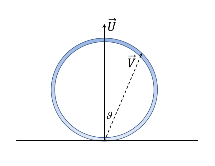
Figure 5: Shell-like structure of $f^{(2)}$ (schematic view of a meridional cross-section of the spherical shell).

In section 6.2 below, we will need a better accuracy than equation (24) provides. Linearizing equation (23) over $\vec{V}^{\prime}$, to first-order accuracy with respect to $V^{\prime}/U\ll 1$, we obtain

$$2\vec{U}\cdot\vec{V}-\left(1+\frac{m}{m_{\beta}}\right)V^{2}+2\left(\frac{m\vec{V}}{m_{\beta}}-\vec{U}\right)\cdot\vec{V}^{\prime}\approx 0.$$

This relation allows expressing small deviations of $V$ from $V_{Q}(\mu)$ in terms of the relatively small velocities $\vec{V}^{\prime}$,

$$V-V_{Q}(\mu)=\frac{m(\vec{q}\cdot\vec{V}^{\prime})}{m_{\beta}\mu U},$$ (26)

where $\vec{q}$ is defined in equation (22).

Using these findings, we will construct an accurate approximation for $\hat{S}_{\mathrm{gain}}[f^{\left(1\right)}]$ given below by equation (33) that will dramatically simplify the solution for $f^{(2)}$.

6.2 Calculation of $\hat{S}_{\mathrm{gain}}[f^{\left(1\right)}]$

In order to calculate the RHS of equation (21) in the employed elastic approximation, $u^{\prime}=u$, we will use for $\hat{S}_{\mathrm{gain}}[f^{\left(1\right)}]$ equation (7a) with $\Delta E_{\mathrm{in}}=0$. This unconventional form of the collisional operator will allow us to avoid complexities associated with expressing the angular arguments of $f^{\left(1\right)}$ in terms of the two scattering angles, $\Theta_{\mathrm{s}}$ and $\Phi_{\mathrm{s}}$. We will calculate $\hat{S}_{\mathrm{gain}}[f^{\left(1\right)}]$ at a given location, characterized by the radius-vector $\vec{R}$, using local velocity variables convenient for the integrations but not necessarily invariants of the collisionless motion.

After integration over $d^{3}V_{\beta}$ and elimination of the momentum conservation $\delta$-function, equation (7a) reduces to

$$\hat{S}_{\mathrm{gain}}[f^{\left(1\right)}]=n_{\mathrm{A}}m\left(1+\frac{m}{m_{\beta}}\right)^{2}\int f^{\left(1\right)}(V^{\prime},\Omega^{\prime})$$

$$\times G\left(u,\Lambda\right)\delta\left(E^{\prime}+\frac{m_{\beta}U^{2}}{2}-E-E_{\beta}\right)\left(V^{\prime}\right)^{2}dV^{\prime}d\Omega^{\prime},$$

where $\Omega^{\prime}$ is the solid angle in the $\vec{V}^{\prime}$-space.

In this velocity space, we introduce an ad hoc spherical system with the major axis parallel to $\vec{R}$. The corresponding variables characterizing $\vec{V}^{\prime}$ are $V^{\prime}$, $\Theta^{\prime}$, $\Phi^{\prime}$, where $\Theta^{\prime}$ and $\Phi^{\prime}$ are the polar and axial angles respectively, so that $d\Omega^{\prime}=d(\cos\Theta^{\prime})d\Phi^{\prime}$. To eliminate the remaining $\delta$-function, instead of a seemingly natural integration over $V^{\prime}$, we will first integrate over $\Phi^{\prime}$ (the benefit of this integration will become clear later). This yields

$$\hat{S}_{\mathrm{gain}}[f^{\left(1\right)}]=mn_{\mathrm{A}}\left(1+\frac{m}{m_{\beta}}\right)^{2}\sum_{i}\int\frac{f^{\left(1\right)}(V^{\prime},\Omega^{\prime})G\left(u,\Lambda\right)\left(V^{\prime}\right)^{2}dV^{\prime}d(\cos\Theta^{\prime})}{\left|\partial E_{\beta}/\partial\Phi^{\prime}\right|_{\Phi^{\prime}=\Phi_{i}^{\prime}}},$$ (27)

where the $i$-summation is over all roots of the energy-conservation equation $E^{\prime}+m_{\beta}U^{2}/2-E-E_{\beta}\left(\Phi^{\prime}\right)=0$ and the derivatives $\partial E_{\beta}/\partial\Phi^{\prime}$ should be calculated before applying this energy conservation. To express $E_{\beta}$ in terms of $\Phi^{\prime}$, we use equation (22) that has followed only from the momentum conservation. This yields

$$E_{\beta}=\frac{m\vec{V}_{\beta}^{2}}{2}=\frac{m^{2}}{m_{\beta}}\left[\frac{(\vec{V}^{\prime})^{2}}{2}-\vec{V}^{\prime}\cdot\vec{q}+\frac{q^{2}}{2}\right],\qquad q\equiv\left|\vec{q}\right|,$$ (28)

where the only $\Phi^{\prime}$-dependent term is $-\vec{V}^{\prime}\cdot\vec{q}$. To find the $\Phi^{\prime}$-dependence, we express $\vec{V}^{\prime}=(\hat{e}_{R}\cos\Theta^{\prime}+\hat{e}_{\Theta}\sin\Theta^{\prime}\cos\Phi^{\prime}+\hat{e}_{\Phi}\sin\Theta^{\prime}\sin\Phi^{\prime})V^{\prime}$ and $\vec{q}=(\hat{e}_{R}\cos\Theta_{q}+\hat{e}_{\Theta}\sin\Theta_{q}\cos\Phi_{q}+\hat{e}_{\Phi}\sin\Theta_{q}\sin\Phi_{q})q$, where $\hat{e}_{R,\Theta,\Phi}$ are the mutually orthogonal base vectors (each unit vector is in the direction of the corresponding coordinate variation). Denoting the angle between $\vec{V}^{\prime}$ and $\vec{q}$ as $\Psi$, we obtain

$$\cos\Psi=\frac{\vec{V}^{\prime}\cdot\vec{q}}{V^{\prime}q}=\cos\Theta^{\prime}\cos\Theta_{q}+\sin\Theta^{\prime}\sin\Theta_{q}\cos(\Phi^{\prime}-\Phi_{q}).$$ (29)

Equations (28) and (29) yield $\left|\partial E_{\beta}/\partial\Phi^{\prime}\right|=\left(m^{2}/m_{\beta}\right)|\partial(\vec{V}^{\prime}\cdot\vec{q})/\partial\Phi^{\prime}|=\left(m^{2}V^{\prime}q/m_{\beta}\right)\left|\sin\Theta^{\prime}\sin\Theta_{q}\sin(\Phi^{\prime}-\Phi_{q})\right|$. The energy-conservation equation, $E^{\prime}+m_{\beta}U^{2}/2-E-E_{\beta}(\Phi_{i}^{\prime})=0$, has exactly two roots $\Phi_{i}^{\prime}$, $i=1,2$, whose specific values are inconsequential for determining $\left|\partial E_{\beta}/\partial\Phi^{\prime}\right|_{\Phi^{\prime}=\Phi_{i}^{\prime}}$. Then using equation (29), we obtain

$$\sum_{i=1}^{2}\frac{\left(\cdots\right)}{\left|\partial E_{\beta}/\partial\Phi^{\prime}\right|_{\Phi^{\prime}=\Phi_{i}^{\prime}}}=\frac{2m_{\beta}\left(\cdots\right)}{m^{2}V^{\prime}q\sqrt{S}},$$ (30)

where the factor ‘$2$’ has originated from the summation over the two roots $\Phi_{i}^{\prime}$ and the function $S$ is given by

$$S\equiv\left|\sin\Theta^{\prime}\sin\Theta_{q}\sin(\Phi^{\prime}-\Phi_{q})\right|^{2}$$

$$=\left[\cos(\Theta_{q}-\Theta^{\prime})-\cos\Psi\right]\times\left[\cos\Psi-\cos(\Theta_{q}+\Theta^{\prime})\right].$$ (31)

Combining equations (27) and (30), we obtain

$$\hat{S}_{\mathrm{gain}}[f^{\left(1\right)}]=\frac{2\left(m+m_{\beta}\right)^{2}n_{\mathrm{A}}}{mm_{\beta}q}\iint\frac{f^{\left(1\right)}(V^{\prime},\Omega^{\prime})G(u,\Lambda)}{\sqrt{S}}\ V^{\prime}dV^{\prime}d(\cos\Theta^{\prime}).$$ (32)

Until this point, all expressions related to $\hat{S}_{\mathrm{gain}}[f^{\left(1\right)}]$ were exact and have not used the smallness of $V^{\prime}/U$ discussed in section 6.1, but now we will use it. To the zero-order accuracy with respect to $V^{\prime}/U$, according to equation (25), we have $u\approx U$ and $\Lambda=\cos\Theta_{\mathrm{sc}}\approx 1-2\mu^{2}$. To the same zeroth order, we have the approximate one-to-one correspondence between $V$ and $\mu$ described by equation (24). This correspondence means that the collisional source of secondary particles, $\hat{S}_{\mathrm{gain}}[f^{\left(1\right)}]$, has an approximate $\delta$-function dependence,

$$\hat{S}_{\mathrm{gain}}[f^{\left(1\right)}]\approx K\delta\left(V-V_{Q}(\mu)\right),\qquad K=\int_{0}^{\infty}\hat{S}_{\mathrm{gain}}[f^{\left(1\right)}]dV,$$ (33)

that corresponds to an infinitely thin shell distribution discussed in section 6.1 and illustrated in Figure 5. However, calculating the factor $K$ requires better accuracy. According to equations (32) and (33), we have

$$K\approx\frac{2\left(m+m_{\beta}\right)^{2}n_{\mathrm{A}}G\left(U,1-2\mu^{2}\right)}{mm_{\beta}q}\int_{0}^{\infty}dV\iint\frac{f^{\left(1\right)}}{\sqrt{S}}\ V^{\prime}dV^{\prime}d\left(\cos\Theta^{\prime}\right)$$

$$=\frac{4\left(m+m_{\beta}\right)^{2}n_{\mathrm{A}}n_{0}G\left(U,1-2\mu^{2}\right)}{\left(2\pi\right)^{3/2}mm_{\beta}qV_{T}^{3}}$$ (34)

$$\!\times\!\!\int_{0}^{\infty}\!\!dV\!\!\iint\mathrm{H}\!\left(\cos\Theta^{\prime}-\sqrt{1-\frac{r_{\mathrm{M}}^{2}}{R^{2}}}\right)\exp\!\left[-\ \frac{\left(V^{\prime}\right)^{2}}{2V_{T}^{2}}-\frac{\nu^{\left(1\right)}R}{V^{\prime}}\right]\!\frac{V^{\prime}dV^{\prime}d\left(\cos\Theta^{\prime}\right)}{\sqrt{S}}.$$

To proceed with the triple integration, we have to first relate $V$ and $\cos\Psi$ defined by equation (29) and contained in the expression for $S$, as defined by equation (31). Only this step requires the first-order expansion with respect to small $V^{\prime}/U$; for anything else it suffices to use the zero-order relation of $V=V_{Q}(\mu)$. Given $\vec{q}$, equation (26) relates the speed difference $(V-V_{Q})$ to the primary-particle velocities $\vec{V}^{\prime}$:

$$\cos\Psi=\frac{\vec{q}\cdot\vec{V}^{\prime}}{qV^{\prime}}\approx\frac{m_{\beta}\mu\left(V-V_{Q}\right)U}{mqV^{\prime}},$$ (35)

so that $dV=[mqV^{\prime}/(m_{\beta}\mu U)]d\left(\cos\Psi\right)$. This yields an interim expression for $K$:

$$K\approx\frac{4n_{\mathrm{A}}n_{0}G\left(U,1-2\mu^{2}\right)}{\left(2\pi\right)^{3/2}\mu V_{T}^{3}U}\left(1+\frac{m}{m_{\beta}}\right)^{2}$$

$$\times\int_{0}^{\infty}\exp\left(-\ \frac{\left(V^{\prime}\right)^{2}}{2V_{T}^{2}}-\frac{\nu^{\left(1\right)}R}{V^{\prime}}\right)\left(V^{\prime}\right)^{2}dV^{\prime}$$

$$\times\iint\mathrm{H}\left(\cos\Theta^{\prime}-\sqrt{1-\frac{r_{\mathrm{M}}^{2}}{R^{2}}}\right)\frac{d(\cos\Theta^{\prime})d(\cos\Psi)}{\sqrt{S}},$$

where the double integration should be performed over the entire 2-D area of positive $S$. First, we integrate over $\cos\Psi$. Using equation (31), we obtain $\left|\int_{\cos\left(\Theta_{q}+\Theta^{\prime}\right)}^{\cos\left(\Theta_{q}-\Theta^{\prime}\right)}d\left(\cos\Psi\right)/\sqrt{S}\right|=\pi$. This exact relation holds even if the two integration limits are infinitesimally close to each other ($\left|\Theta^{\prime}\right|\rightarrow 0$). Then, integrating over $\cos\Theta^{\prime}$, we obtain

$$K(\mu,R) \approx\sqrt{\frac{2}{\pi}}\ \frac{n_{\mathrm{A}}n_{0}G\left(U,1-2\mu^{2}\right)}{\mu U}\left(1+\frac{m}{m_{\beta}}\right)^{2}\left(1-\sqrt{1-\frac{r_{\mathrm{M}}^{2}}{R^{2}}}\right)Z(\eta)$$

$$\approx\frac{2n_{\mathrm{A}}n_{0}G\left(U,1-2\mu^{2}\right)}{\sqrt{3}\ \mu U}\left(1+\frac{m}{m_{\beta}}\right)^{2}\left[1+\left(\frac{\nu^{\left(1\right)}R}{V_{T}}\right)^{2/3}\right]$$

$$\times\left(1-\sqrt{1-\frac{r_{\mathrm{M}}^{2}}{R^{2}}}\right)\exp\left[-\ \frac{3}{2}\left(\frac{\nu^{\left(1\right)}R}{V_{T}}\right)^{2/3}\right],$$ (36)

where in the latter, approximate, equality the dimensionless integral,

$$Z(\eta)\equiv\frac{1}{V_{T}^{3}}\int_{0}^{\infty}\exp\left(-\ \frac{V^{2}}{2V_{T}^{2}}-\frac{\nu^{\left(1\right)}R}{V}\right)V^{2}dV$$ (37)

$$=\left(2\eta\right)^{\frac{3}{2}}\int_{0}^{\infty}\exp\left[-\eta\left(x^{2}+\frac{2}{x}\right)\right]x^{2}dx,\qquad\eta=\frac{1}{2}\left(\frac{\nu^{\left(1\right)}R}{V_{T}}\right)^{\frac{2}{3}},$$

was approximated by its $R\gg\lambda^{(1)}$ ($\eta\gg 1$) asymptotic expression,

$$\left.Z\right|_{\eta\gg 1}\approx\sqrt{\frac{2\pi}{3}}\left(1+2\eta\right)e^{-3\eta}.$$ (38)

Approximate equation (38) works reasonably well for all distances from the meteoroid center, even in the worst case of $R\ll\lambda_{T}^{(1)}$ when approximate $Z(\eta)$ exceeds the exact expression by a factor of $2/\sqrt{3}\approx 1.155$, as shown in Figure 6.

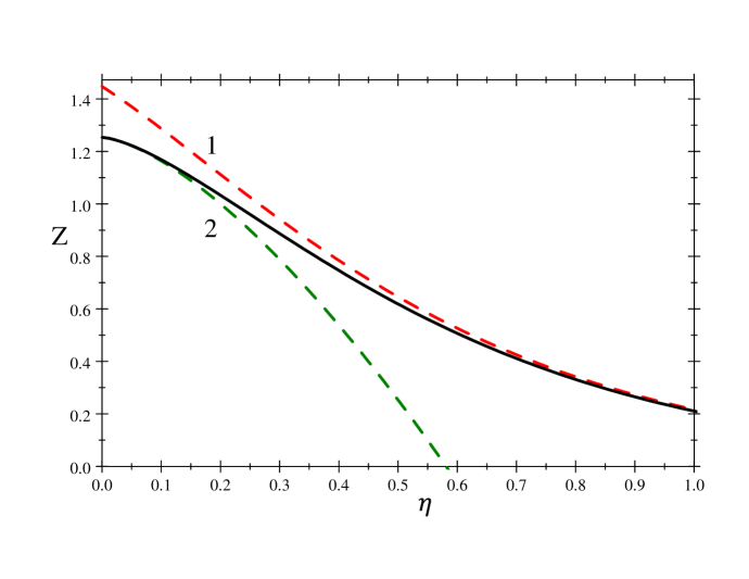
Figure 6: Function $Z(\eta)$ defined by equation (37). The solid curve shows the result of exact computer integration, while the dashed curves show the corresponding large-$\eta$ and small-$\eta$ asymptotics: (1) $\left.Z\right|_{\eta\gg 1}$ given by equation (38) and (2) $\left.Z\right|_{\eta\ll 1}\approx\sqrt{\pi/2}-2\sqrt{2}\ \eta^{\frac{3}{2}}$.

Thus the ‘gain’ term for the secondary particles, $\hat{S}_{\mathrm{gain}}[f^{\left(1\right)}]$, is given by equation (33), where the factor $K(\mu,R)$ is given by equation (36). One can verify that $\hat{S}_{\mathrm{gain}}[f^{\left(1\right)}]$ satisfies equation (17). Since $V$ and $\mu$ are invariants of the particle collisionless motion, the approximate $\delta$-function speed dependence of equation (33) translates to a similar $V,\mu$-dependence for $f^{\left(2\right)}$, as described in equation (41) below.

6.3 Integration over particle trajectories

Having calculated the RHS of equation (21), we are ready to solve it by characteristics. Because the LHS of equation (21) contains spatial derivatives we should use the coordinate system appropriate for the assumed axial symmetry around the direction of $\vec{U}$ and employ invariant variables in the velocity space. The RHS of (21) depends only on one spatial coordinate, $R$, so it is convenient to use for the real space the spherical coordinate system: $R$, $\theta$, and $\phi$, where $\theta$ is the polar angle with respect to the $\vec{U}$-direction and $\phi$ is the corresponding axial angle (due to the axial symmetry, there will be no $\phi$-dependence). Positive values of $\cos\theta=(\vec{R}\cdot\vec{U})/(RU)$ denote locations behind the descending meteoroid, while negative $\cos\theta$ denote locations in front of it. Similar to section 5, we will use the minimum distance of a given straight-line particle trajectory to the meteoroid center, $R_{0}=R\sin\Theta$, as one of the velocity-space variables that remain invariant during the particle free motion, see Figure 3. The entire set of these invariant variables includes $V$, $R_{0}$, and $\Phi$, where the axial angle $\Phi$ is the axial angle of $\vec{V}$ measured around the direction of $\vec{R}$ from the common $\vec{R}$-$\vec{U}$ plane. We should bear in mind that the polar angle in the velocity space, $\Theta$, measured from the local direction of $\vec{R}$ is not an invariant of the free particle motion.

In these variables, using the approximation given by equation (33), we reduce equation (21) without the $\nu^{(2)}f^{\left(2\right)}$ term to

$$V_{R}(R,V)\ \frac{df^{\left(2\right)}}{dR}=K\left(\mu,R\right)\delta\left(V-V_{Q}\left(\mu\right)\right),$$ (39)

where $V_{Q}\left(\mu\right)$ is defined by equation (24) and $K\left(\mu,R\right)$ by equation (36). In the LHS of equation (39), $d/dR$ denotes the full derivative along a given particle trajectory characterized by $V$, $R_{0}$, $\Phi$, with the $R$-dependent local radial component of the particle velocity, $V_{R}$, given by

$$V_{R}\equiv V\cos\Theta=\sigma_{R}\sqrt{1-\frac{R_{0}^{2}}{R^{2}}}\ V,\qquad\sigma_{R}=\pm 1.$$ (40)

Here $\sigma_{R}$ is an additional discrete parameter which identifies either ‘outgoing’ ($dR/dt>0$, $\sigma_{R}=+1$) or ‘incoming’ ($dR/dt<0$, $\sigma_{R}=-1$) particles, as depicted in Figure 3. The parameter $\sigma_{R}$ remains invariant until the particle passes the minimum distance between the trajectory and the meteoroid center, $R_{0}$. After this the negative sign of $\sigma_{R}$ switches to the positive one, i.e., the incoming particle becomes outgoing. At a given location characterized by $R$, $\theta$ with the given velocity-space parameters $V$, $R_{0}$, $\Phi$, the entire velocity distribution is composed of two distinct partial  distributions: one for the incoming particles and the other for the outgoing particles. They correspond to particles arriving from the two opposite directions. We will distinguish these two distributions by the corresponding subscripts, $f_{\sigma_{R}}^{\left(2\right)}=f_{\pm}^{\left(2\right)}$. Note that the functions $f_{+}^{\left(2\right)}$ and $f_{-}^{\left(2\right)}$ can be vastly different. For example, the primary meteoric particles are exclusively outgoing, so that $f_{-}^{\left(1\right)}=0$. Any incoming particles appear only due to collisions.

The characteristics of equation (39) are straight-line particle trajectories characterized by $V$, $R_{0}$, $\Phi$ and arriving at a given location $R$, $\theta$ from the direction determined by $\sigma_{R}$. To distinguish the fixed coordinate $R$ from flowing coordinates along a given trajectory we will denote the latter by $R^{\prime}$ with corresponding $V_{R^{\prime}}$ and $\sigma_{R^{\prime}}$. As discussed in section 6.1, for almost the entire secondary-particle population $\mu=\cos\vartheta$ is positive, so that all relevant particle trajectories start in front of the descending meteoroid sufficiently far from it, where there are virtually no sheath particles.

We can write the formal solution of equation (39) as

$$f_{\sigma_{R}}^{\left(2\right)}\approx\frac{1}{V}\ \delta\left(V-\frac{2\mu m_{\beta}U}{m+m_{\beta}}\right)\int_{\infty}^{R}\frac{K\left(\mu,R^{\prime}\right)R^{\prime}dR^{\prime}}{\sigma_{R^{\prime}}\sqrt{(R^{\prime})^{2}-R_{0}^{2}}}.$$ (41)

where the lower integration limit denotes an infinitely far distance in front of the descending meteoroid. This schematic expression, however, needs a refinement associated with the fact that the spherical radius $R^{\prime}$ is a non-monotonic function of the particle position along its trajectory. For the incoming particles with $\sigma_{R}=-1$, the radial distance $R^{\prime}$ is monotonically decreasing, so that along the entire particle trajectory we have $\sigma_{R^{\prime}}=-1$. In contrast, for the outgoing particles ($\sigma_{R}=+1$) arriving at a given location $R$, the radial distance $R^{\prime}$ first decreases ($\sigma_{R^{\prime}}=-1$) from $\infty$ down to the minimum distance $R^{\prime}=R_{0}$ and then starts increasing again ($\sigma_{R^{\prime}}=+1$) until it reaches $R^{\prime}=R$. As a result, the integral in equation (41) leads to a piecewise expression:

$$\int_{\infty}^{R}\frac{K\left(\mu,R^{\prime}\right)R^{\prime}dR^{\prime}}{\sigma_{R^{\prime}}\sqrt{(R^{\prime})^{2}-R_{0}^{2}}}=\left\{\!\!\begin{array}[c]{ccc}\int_{R}^{\infty}\frac{K\left(\mu,R^{\prime}\right)R^{\prime}dR^{\prime}}{\sqrt{\left(R^{\prime}\right)^{2}-R_{0}^{2}}}&\text{if}&\sigma_{R}=-1,\\ &&\\ \int_{R_{0}}^{R}\frac{K\left(\mu,R^{\prime}\right)R^{\prime}dR^{\prime}}{\sqrt{\left(R^{\prime}\right)^{2}-R_{0}^{2}}}\ {\normalsize+}\int_{R_{0}}^{\infty}\frac{K\left(\mu,R^{\prime}\right)R^{\prime}dR^{\prime}}{\sqrt{\left(R^{\prime}\right)^{2}-R_{0}^{2}}}&\text{if}&\sigma_{R}=+1.\end{array}\right.$$ (42)

Another important issue is that the secondary particles have only positive values of $\mu=\cos\vartheta=(\vec{V}\cdot\vec{U})/(VU)$, as described in section 6.1; otherwise $f_{\sigma_{R}}^{\left(2\right)}=0$. The invariant parameter $\mu$ can be expressed in terms of the spherical coordinates, $R$, $\theta$, and velocity-space variables, $R_{0}$, $\Phi$, $\sigma_{R}$, as

$$\mu\equiv\cos\vartheta=\cos\Theta\cos\theta+\sin\Theta\sin\theta\cos\Phi$$

$$=\sigma_{R}\sqrt{1-\frac{R_{0}^{2}}{R^{2}}}\ \cos\theta+\frac{R_{0}\sin\theta}{R}\ \cos\Phi.$$ (43)

The boundary $\mu=0$ corresponds to the critical value of $R_{0}=R_{c}(\Phi)$,

$$R_{c}(\Phi)=\frac{R\left|\cos\theta\right|}{\sqrt{\cos^{2}\theta+\sin^{2}\theta\cos^{2}\Phi}}=\frac{R\left|\cos\theta\right|}{\sqrt{1-\sin^{2}\theta\sin^{2}\Phi}}.$$ (44)

Figure 7 shows $R_{c}(\Phi)/R$ for a few values of $\theta$. As $\theta\rightarrow 0,\pi$ the entire function $R_{c}(\Phi)$ approaches $R$. As $\theta\rightarrow\pi/2$ the function approaches $0$ everywhere except narrow spikes near $\Phi=\pm\pi/2$ where $R_{c}=R$. Behind the descending meteoroid, where $\cos\theta>0$, we have $f_{\sigma_{R}}^{\left(2\right)}=0$ for $\sigma_{R}=+1$ within $0<R_{0}<R_{c}(\Phi)$ and for $\sigma_{R}=-1$ within $R_{c}(\Phi)<R_{0}<R$. In front of the meteoroid, where $\cos\theta<0$, on the contrary, $f_{\sigma_{R}}^{\left(2\right)}=0$ for $\sigma_{R}=+1$ within $R_{c}(\Phi)<R_{0}<R$ and for $\sigma_{R}=-1$ within $0<R_{0}<R_{c}(\Phi)$.

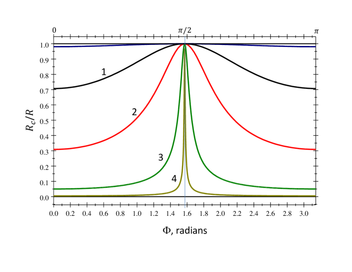
Figure 7: The function $R_{c}(\Phi)/R$ for several values of $\theta$: curve 1 for $\theta=\pi/4$, curve 2 for $\theta=3\pi/5$, curve 3 for $\theta=\pi/2-0.05\approx 1.5208$, curve 4 for $\theta=\pi/2-0.005\approx 1.5658$.

As a result, given the particle coordinates in real space, $R$, $\theta$, with the velocity parameters, $R_{0}=R\sin\Theta$, $\Phi$, $\sigma_{R}$, and using the explicit expression for $K\left(\mu,R^{\prime}\right)$ given by equation (36), we obtain:

$$f_{\sigma_{R}}^{(2)}=L_{\sigma_{R}}\ \delta\left(V-\frac{2m_{\beta}\mu U}{m+m_{\beta}}\right),$$

$$L_{\sigma_{R}} =\frac{G(U,1-2\mu^{2})n_{0}n_{\mathrm{Atm}}}{\sqrt{3}\ \mu U^{2}}\left(1+\frac{m}{m_{\beta}}\right)^{3}I(R,R_{0})$$ (45)

if, concurrently,

$$\sigma_{R}=\mathrm{sgn}(\cos\theta)\qquad\text{and}\qquad 0<R_{0}<R_{c}(\Phi)$$ (46a)

or

$$\sigma_{R}=-\mathrm{sgn}(\cos\theta)\qquad\text{and}\qquad R_{c}(\Phi)<R_{0}<R.$$ (46b)

Otherwise (i.e., if $\mu<0$), $f_{\sigma_{R}}^{\left(2\right)}=0$. In accord with equation (42), the multiplier $I(R,R_{0})$ in (45), has a piecewise definition

$$I(R,R_{0})=\left\{\begin{array}[c]{ccc}J_{R}^{\infty}&\text{for}&\sigma_{R}=-1\\ &&\\ J_{R_{0}}^{\infty}\mathrm{H}\left(R_{0}-r_{\mathrm{M}}\right)+J_{\max\left(R_{0},r_{\mathrm{M}}\right)}^{R}&\text{for}&\sigma_{R}=+1,\end{array}\right.$$ (47)

where the integral $J_{a}^{b}$, as a function of its integration limits, $b>a\geq R_{0}$, is defined by

$$J_{a}^{b}\equiv 2\int_{a}^{b}\left(1-\sqrt{1-\frac{r_{\mathrm{M}}^{2}}{\left(R^{\prime}\right)^{2}}}\right)\left[1+\left(\frac{R^{\prime}}{\lambda^{(1)}}\right)^{2/3}\right]$$

$$\times\exp\left[-\ \frac{3}{2}\left(\frac{R^{\prime}}{\lambda^{(1)}}\right)^{2/3}\right]\frac{R^{\prime}dR^{\prime}}{\sqrt{\left(R^{\prime}\right)^{2}-R_{0}^{2}}}\ .$$ (48)

The first line in the RHS of equation (47) describes incoming particles that arrive at a given location $\vec{R}$ after being scattered or ionized within the segment of a given straight-line trajectory located between an infinitely large distance (in front of the descending meteoroid) and $\vec{R}$. The second line in the RHS of equation (47) describes outgoing particles that arrive along a different line segment from the opposite direction. The first term, $J_{R_{0}}^{\infty}\mathrm{H}\left(R_{0}-r_{\mathrm{M}}\right)$, describes secondary particles originated in the beginning part of the straight-line trajectory, from an infinitely large distance down to the minimum distance $R_{0}$. In this part of the trajectory the particles were incoming. The second term, $J_{R_{0}}^{R}$, describes the outgoing particles originated within the remaining part of this trajectory $R$, as illustrated by Figure 3. The step-function $\mathrm{H}\left(R_{0}-r_{\mathrm{M}}\right)$ and $\max\left(R_{0},r_{\mathrm{M}}\right)$ there are associated with particle trajectories that may cross the meteoroid surface, $R_{0}<r_{\mathrm{M}}$. Such trajectories always exist, regardless of how far from the meteoroid is the given location $\vec{R}$. For the trajectories with $R_{0}<r_{\mathrm{M}}$, the meteoroid surface shields all outgoing particles arriving at $\vec{R}$ from the opposite side of the meteoroid. This shielding will inevitably lead to a dip in the velocity distribution of the outgoing particles, $f_{+}^{(2)}$, with a discontinuity at $R_{0}=r_{\mathrm{M}}$.

The velocity distribution of secondary particles that originated in close proximity to the meteoroid is sensitive to the actual meteoroid shape. The latter can be far from spherical, and even more so, the actual boundary conditions on the meteoroid surface may include inelastic reflections of the impinging particles from chaotically distributed surface irregularities. In this case, the anticipated dip in $f_{+}^{(2)}$ might be, at least partially, filled with such reflected particles. Since we do not have a detailed knowledge of these conditions, we will stick to the simplest case of the ideally spherical meteoroid with the fully absorbing surface. We will also ignore local disturbances of the neutral atmosphere that are caused by the falling meteoroid itself.

In equation (48), the integral $J_{a}^{b}$ is analytically intractable and needs approximations. Presenting $J_{\max\left(R_{0},r_{\mathrm{M}}\right)}^{R}$ as the difference of two well-convergent improper integrals, $J_{\max\left(R_{0},r_{\mathrm{M}}\right)}^{R}=J_{\max\left(R_{0},r_{\mathrm{M}}\right)}^{\infty}-J_{R}^{\infty}$, we restrict our analysis to $J_{a}^{\infty}$, where the lower integration limit, $a$, equals $R$, $R_{0}$, or $r_{\mathrm{M}}$. These integrals allow analytical approximations due to the fact that the mean free path of the primary particles, $\lambda^{(1)}$, is many orders of magnitude larger than the meteoroid size, $r_{\mathrm{M}}$. This allows separating the entire domain of parameters $R$ and $R_{0}$ into overlapped sub-domains where the integral (48) becomes simpler. On the one hand, for relatively large $a\gg r_{\mathrm{M}}$, including $a\gtrsim\lambda^{(1)}$, the first factor in the integrand of (48) allows the Taylor expansion $2(1-\sqrt{1-r_{\mathrm{M}}^{2}/(R^{\prime})^{2}}\ )\approx r_{\mathrm{M}}^{2}/(R^{\prime})^{2}$. This expansion works well even under a much weaker condition of $R^{\prime}\gtrsim 3r_{\mathrm{M}}$. On the other hand, for relatively short distances from the meteoroid center, $R_{0}\leq R\ll\lambda^{(1)}$, including $R_{0}\lesssim r_{\mathrm{M}}$, in the entire range of $R^{\prime}\gtrsim\lambda^{(1)}$ the integrand of (48) is small and makes no tangible contribution to the total integral value, while for $R^{\prime}\ll\lambda^{(1)}$ one can neglect the terms involving $(R^{\prime}/\lambda^{(1)})^{2/3}$. This allows the remaining integral to be expressed in terms of the elliptic integrals. Below we calculate $J_{a}^{\infty}$ separately for each sub-domain.

Near zone: $r_{\mathrm{M}}\leq R\ll\lambda^{(1)}$.

The corresponding integrals are calculated in the appendix in terms of the elliptic integrals. This calculation yields

$$J_{R}^{\infty}\approx\left\{\begin{array}[c]{ccc}2r_{\mathrm{M}}\mathrm{E}\left(\frac{r_{\mathrm{M}}}{R};\frac{R_{0}}{r_{\mathrm{M}}}\right)-2\sqrt{R^{2}-R_{0}^{2}}\left(1-\sqrt{1-\frac{r_{\mathrm{M}}^{2}}{R^{2}}}\right)&\text{if}&R_{0}\leq r_{\mathrm{M}}\\ &&\\ \begin{array}[c]{c}2R_{0}\left[\mathrm{E}\left(\frac{R_{0}}{R};\frac{r_{\mathrm{M}}}{R_{0}}\right)-\left(1-\frac{r_{\mathrm{M}}^{2}}{R_{0}^{2}}\right)\ \mathrm{F}\left(\frac{R_{0}}{R};\frac{r_{\mathrm{M}}}{R_{0}}\right)\right]\\ \\ -\ 2\left(1-\sqrt{1-\frac{r_{\mathrm{M}}^{2}}{R^{2}}}\right)\sqrt{R^{2}-R_{0}^{2}}\end{array}&\text{if}&R_{0}\geq r_{\mathrm{M}},\end{array}\right.$$ (49)

and

$$J_{\max\left(R_{0},r_{\mathrm{M}}\right)}^{\infty}\approx\left\{\begin{array}[c]{ccc}2r_{\mathrm{M}}\mathrm{E}\left(\frac{R_{0}}{r_{\mathrm{M}}}\right)-2\sqrt{r_{\mathrm{M}}^{2}-R_{0}^{2}}&\text{if}&R_{0}\leq r_{\mathrm{M}}\\ &&\\ 2R_{0}\left[\mathrm{E}\left(\frac{r_{\mathrm{M}}}{R_{0}}\right)-\left(1-\frac{r_{\mathrm{M}}^{2}}{R_{0}^{2}}\right)\mathrm{K}\left(\frac{r_{\mathrm{M}}}{R_{0}}\right)\right]&\text{if}&R_{0}\geq r_{\mathrm{M}},\end{array}\right..$$ (50)

Intermediate sub-domain: $3r_{\mathrm{M}}\lesssim R_{0}\leq R\ll\lambda^{(1)}$.

These conditions enable the easiest calculation of $J_{a}^{\infty}$ and, at the same time, they cover a rather broad parameter sub-domain. Using simultaneously both Taylor expansions described above and restricting them to the highest-order terms, we arrive at fairly simple expressions:

$$J_{R}^{\infty}\approx\frac{r_{\mathrm{M}}^{2}}{R_{0}}\ \arcsin\frac{R_{0}}{R},\qquad J_{\max\left(R_{0},r_{\mathrm{M}}\right)}^{\infty}=J_{R_{0}}^{\infty}\approx\frac{\pi r_{\mathrm{M}}^{2}}{2R_{0}}.$$ (51)

Long-distance/large-$R_{0}$ zone: $R\geq R_{0}\gg r_{\mathrm{M}}$.

In this sub-domain, we should keep all the factors with $(R_{0}/\lambda^{(1)})^{2/3}$, but can use the Taylor expansion $2(1-\sqrt{1-r_{\mathrm{M}}^{2}/(R^{\prime})^{2}})\approx r_{\mathrm{M}}^{2}/(R^{\prime})^{2}$. Then we temporarily recast $J_{a}^{\infty}$ with $a\gg r_{\mathrm{M}}$ as

$$J_{a}^{\infty}=\frac{r_{\mathrm{M}}^{2}I_{\alpha}^{\infty}}{R_{0}},\qquad I_{\alpha}^{\infty}\left(\Lambda\right)=\int_{\alpha}^{\infty}\left(\Lambda+\frac{3}{2y}\right)\frac{e^{-\Lambda y}dy}{\sqrt{y^{3}-1}},$$ (52)

where

$$y\equiv\left(\frac{R^{\prime}}{R_{0}}\right)^{2/3},\qquad\alpha\equiv\left(\frac{a}{R_{0}}\right)^{2/3},\qquad\Lambda\equiv\frac{3}{2}\left(\frac{R_{0}}{\lambda_{T}^{(1)}}\right)^{2/3}.$$ (53)

In the limit of $\Lambda\alpha\ll 1$ corresponding to $a\gg r_{\mathrm{M}}$, by changing variable $y=(1+z^{2})^{1/3}$ one can easily verify that equation (52) yields (51).

Calculating the integral $I_{\alpha}^{\infty}\left(\Lambda\right)$ in limiting cases and interpolating between those, we construct the following approximation,

$$I_{\alpha}^{\infty}\left(\Lambda\right)\approx\frac{e^{-\Lambda\alpha}}{\sqrt{\alpha^{3}-1+\left[\pi\left(\frac{\Lambda}{3}+\frac{\pi}{4}\right)\right]^{-1}}}.$$ (54)

Direct numeric calculations show that the maximum discrepancy between the exact value of the integral and that given by equation (54) is near $\alpha\simeq 1.06$, where it reaches $\simeq 12\%$; in most other occasions this discrepancy is much smaller. In the original notations, equation (54) yields

$$J_{R}^{\infty}\approx\frac{r_{\mathrm{M}}^{2}\sqrt{1+\frac{2}{\pi}\left(\frac{R_{0}}{\lambda_{T}^{(1)}}\right)^{2/3}}\exp\left[-\ \frac{3}{2}\left(\frac{R}{\lambda_{T}^{(1)}}\right)^{2/3}\right]}{\sqrt{\left[1+\frac{2}{\pi}\left(\frac{R_{0}}{\lambda_{T}^{(1)}}\right)^{2/3}\right]\left(R^{2}-R_{0}^{2}\right)+\frac{4R_{0}^{2}}{\pi^{2}}}}.$$ (55)

Setting in equation (55) $R=R_{0}$, we obtain

$$J_{\max(R_{0},r_{\mathrm{M}})}^{\infty}=J_{R_{0}}^{\infty}\approx\frac{\pi r_{\mathrm{M}}^{2}}{2R_{0}}\sqrt{1+\frac{2}{\pi}\left(\frac{R_{0}}{\lambda_{T}^{(1)}}\right)^{2/3}}\exp\left[-\ \frac{3}{2}\left(\frac{R_{0}}{\lambda_{T}^{(1)}}\right)^{2/3}\right].$$ (56)

For $R_{0}\ll R\ll\lambda_{T}^{(1)}$, these expressions agree with the intermediate asymptotics given by equation (51). These equations give the expressions for $J_{R}^{\infty}$ and $J_{R_{0}}^{\infty}\mathrm{H}\left(R_{0}-r_{\mathrm{M}}\right)+J_{\max\left(R_{0},r_{\mathrm{M}}\right)}^{R}$, where $J_{\max\left(R_{0},r_{\mathrm{M}}\right)}^{R}=J_{\max\left(R_{0},r_{\mathrm{M}}\right)}^{\infty}-J_{R}^{\infty}$, to be substituted first in equation (47) and then to (45) for calculating $f_{\sigma_{R}}^{(2)}$.

All the above relations are expressed in terms of the invariant variables $R_{0}$, $\mu,$ and $V$. For applications, it is more convenient to express $R_{0}$ in terms of the polar angle in velocity space, $\Theta$, around the local radius-vector $\vec{R}$ direction, $R_{0}=R\sin\Theta$. One might also need to express $\mu$ in terms of $\Theta$ and the corresponding axial angle, $\Phi$ (measured from the common $\vec{R}$-$\vec{U}$ plane), $\mu\equiv\cos\vartheta=\cos\Theta\cos\theta+\sin\Theta\sin\theta\cos\Phi$, where $\theta$ is the polar angle in real space measured from the direction of $\vec{U}$.

Figures 8, 9, and 10 illustrate $f_{\sigma_{R}}^{(2)}$ given by equation (45). In the entire 3-D velocity space, the distribution function has a shell-like structure depicted by Figure 5 and approximated by the $\delta$-function. Below we show the angular dependence of the factor $L_{\sigma_{R}}$ preceding the $\delta$-function and defined by equation (45).

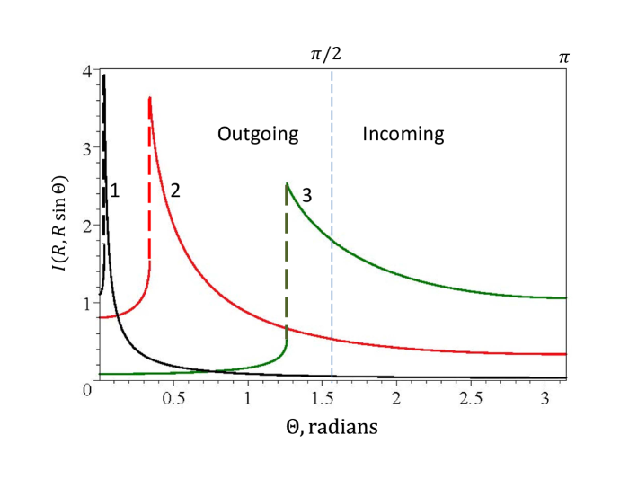
Figure 8: The factor $I(R,R_{0})$ with $R_{0}=R\sin\Theta$ for several distances from the meteoroid surface: curve 1 for $R=30r_{\mathrm{M}}$, curve 2 for $R=3r_{\mathrm{M}}$, curve 3 for $R=1.05r_{\mathrm{M}}$. The dashed line segments of each curve indicate trajectories tangential to the meteoroid surface, $R\sin\Theta=r_{\mathrm{M}}$. For $\Theta<\Theta_{c}=\arcsin(r_{\mathrm{M}}/R)$, a significant fraction of particles moving along the corresponding straight-line trajectory are shielded by the meteoroid and cannot reach the destination point. This shielding produces the pronounced dips for all $\Theta<\Theta_{c}$. Notice the smooth transition between the outgoing and incoming particles at $\Theta=\pi/2$.

We start from the function $I(R,R_{0})=I(R,R\sin\Theta)$ which is the major $\Theta$-dependent multiplier in the expression for $L_{\sigma_{R}}(\Theta,\Phi)$. Figure 8 shows $I(R,R\sin\Theta)$ as a function of $\Theta$ for several radial distances $R$. Each curve combines $I$ for the outgoing particles, $\sigma_{R}=+1$, with that for the incoming particles, $\sigma_{R}=-1$. For the outgoing ($0\leq\Theta\leq\pi/2$) and incoming ($\pi/2\leq\Theta\leq\pi$) particles, equation (47) gives different analytic expressions, but they match at $\Theta=\pi/2$ smoothly. At $\Theta=\Theta_{\mathrm{cr}}\equiv\arcsin(r_{\mathrm{M}}/R)$, the distribution function undergoes a discontinuity corresponding to the boundary between the unhindered particle trajectories and those with particles shielded by the meteoroid, $R_{0}=r_{\mathrm{M}}$, as we discussed above. The function $I(R,R\sin\Theta)$ reaches its maximum at $\Theta=\Theta_{\mathrm{cr}}$. For $R\gg r_{\mathrm{M}}$, the outgoing particles form a spiky angular distribution at small $\Theta\lesssim r_{\mathrm{M}}/R$ corresponding to almost radially propagating particles, $\vartheta\approx\theta$. As $R$ becomes large, the narrower this angular spike becomes.

Figure 7 corresponds to distances $R\ll\lambda_{T}^{(1)}$, but for $R\gtrsim\lambda_{T}^{(1)}$ the angular distribution of $I(R,R\sin\Theta)$ is qualitatively the same, although resolving the narrow spike on the corresponding diagram would be hard. The spike about the direction of the radius-vector $\vec{R}$ occurs because the source density for the secondary particles is proportional to the density of the primary particles, $n^{(1)}\propto 1/(R^{\prime})^{2}$, and hence is largest near the meteoroid surface.

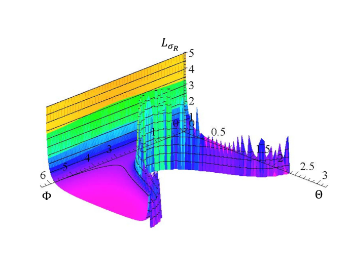
Figure 9: The factor $L_{\sigma_{R}}$ defined by equation (45), as a function of local polar ($\Theta$) and axial ($\Phi$) angles in the velocity space, for a location partially behind the descending meteoroid, $\theta=\pi/4$ (the 3-D surface plot is cut off vertically).

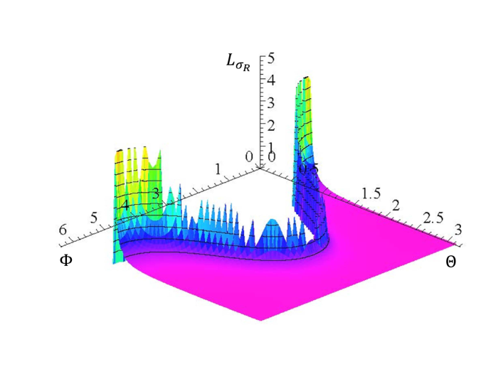
Figure 10: The factor $L_{\sigma_{R}}$ defined by equation (45), as a function of local polar ($\Theta$) and axial ($\Phi$) angles in the velocity space, for a location partially in front of the descending meteoroid, $\theta=3\pi/4$ (the 3-D surface plot is cut off vertically).

Figures 9 and 10 show two examples of the full factor $L_{\sigma_{R}}(\Theta,\Phi)$ plotted as a 3-D surface over the entire $\Theta$,$\Phi$-domain: $0\leq\Theta\leq\pi$, $0\leq\Phi\leq 2\pi$. Each plot combines $L_{\sigma_{R}}(\Theta,\Phi)$ for the outgoing particles, $L_{+}$ ($0\leq\Theta\leq\pi/2$) with that for the incoming particles, $L_{-}$ ($\pi/2\leq\Theta\leq\pi$). Following $I(R,R\sin\Theta)$, the two surfaces of $L_{\pm}(\Theta,\Phi)$ match smoothly at $\Theta=\pi/2$. The two different 3-D plots correspond to the same radial distance ($R=30r_{\mathrm{M}}$), but different values of the polar angle in real space, $\theta$. One corresponds to an axially symmetric location behind the descending meteoroid ($\theta=\pi/4$), while the other to a similar location in front of it ($\theta=3\pi/4$). For simplicity, we assumed an isotropic differential cross-section, $G(U,1-2\mu^{2})=G(U)$. The non-zero values of $L_{\sigma_{R}}$ occupy a part of the entire $\Theta$,$\Phi$-domain bounded by $\Theta=0$, $0\leq\Phi\leq 2\pi$ and the $\Theta$,$\Phi$-curve determined by $\mu=\cos\Theta\cos\theta+\sin\Theta\sin\theta\cos\Phi=0$ (this curve corresponds to $R_{0}=R_{c}(\Phi)$ in Figure 7). Near these two boundaries, the plotted surface has two pronounced ‘ridges’ (for better visualization, they are cut off vertically). The ‘ridge’ near $\Theta=0$ is formed by the spiky maximum of $I(R,R\sin\Theta)$ for the outgoing particles, $L_{+}$, as discussed above. The ‘ridge’ near $\mu=0$ is associated with the singular factor $\mu$ in the denominator of (45). As we discuss in the companion paper, this singularity plays no role for the total plasma density or flux because the corresponding integrals of $f_{\sigma_{R}}^{(2)}$ include weighting factors that not only suppress the singularity, but make its contribution negligible.

The ‘ridge’ near $\Theta=0$ is different. Its tallest part with $\Theta\lesssim 3r_{\mathrm{M}}/R$ corresponding to $R_{0}\lesssim 3r_{\mathrm{M}}$ comes from trajectories passing through a small volume near the meteoroid surface where the density of the primary particles increases $\propto 1/(R^{\prime})^{2}$. This part of the distribution function is described by more complicated equations (49) and (50). However, for most locations with $R\gg r_{\mathrm{M}}$, particles with $\Theta\lesssim 3r_{\mathrm{M}}/R$ cannot make significant contributions to the total particle density and flux because the contribution of secondary particles originated beyond the near-meteoroid volume are $\sim\lambda_{T}^{(1)}/r_{\mathrm{M}}$ times larger. These particles form a ‘pedestal’ in the $\Theta$-distribution of secondary particles which at large distances $R$ is localized, $\Theta\lesssim\lambda_{T}^{(1)}/R$, but much broader than the central spike of $\Theta\lesssim 3r_{\mathrm{M}}/R$. The fact that in spite of the much higher density of primary particles directly near the meteoroid, $R^{\prime}\lesssim 3r_{\mathrm{M}}$, the majority of secondary particles exists within a large volume $r_{\mathrm{M}}\ll R^{\prime}\lesssim\lambda_{T}^{(1)}$. The scattering or ionization of the primary particles is described by the exponential factor $\propto\exp[-(3/2)(R^{\prime}/\lambda_{T}^{(1)})^{2/3}]$ in equation (48). This exponential loss of $\ll$primary particles represents the entire source for the secondary particles. Hence the volume with $R^{\prime}\ll\lambda_{T}^{(1)}$ with almost no exponential loss cannot be the dominant source of secondary particles.

7 Summary and conclusions

We have developed a first-principle collisional kinetic model of plasma and neutral sheath formed around a fast-descending small meteoroid when it passes the altitude range of 90-120 km. In this range, sensitive radars detect atmospheric effects of the meteoroid passage and we will use this theory to more accurately interpret the radar head echo (Close et al., 2005; Campbell-Brown and Close, 2007). The analytic theory of this paper describes the spatial structure and velocity distributions of heavy particles: ions and neutral particles of the meteoric origin, while electrons are assumed to roughly follow the Boltzmann distribution.

The velocity distribution of the neutral ‘primary’ particles, $f^{(1)}$, is given by equation (19), but the central topic of this paper is finding the velocity distributions of the ‘secondary’ particles, $f^{(2)}$, where we have also included all higher-order subgroups, $f^{(j)}$ with $j>2$. These distributions are described by equations (45) and (47). If $3r_{\mathrm{M}}\lesssim R_{0}\leq R\ll\lambda_{T}^{(1)}$ then $J_{a}^{\infty}$ reduce to simple equation (51). An important feature of the ‘secondary’-particle distribution functions $f_{\sigma_{R}}^{(2)}$ ($\sigma_{R}=\pm 1$) is their shell-like distribution in velocity space, approximately described in equation (45) by the $\delta$-function factor and illustrated by Figure 5. Such anisotropic and non-monotonic velocity distributions are potentially unstable and may give rise to detectable plasma turbulence. However, analysis of kinetic plasma instabilities in the near-meteoroid plasma may require a more accurate description of electrons.

In the companion paper, we apply this kinetic theory to calculate a spatial structure of the near-meteoroid plasma. This will allow accurate modeling of radar head echoes. Our future work will include a more detailed and specific theoretical analysis, computer simulations, and discussion of implications for real meteors and comparisons with radar and other observations.

Appendix A Derivation of kinetic equation (5)

We start with the collisional kinetic equation for $f(\vec{V},\vec{r})$ in a general probabilistic form (Lifshitz and Pitaevskii, 1981),

$$\frac{\partial}{\partial t}+\vec{V}\cdot\nabla+\frac{\vec{F}}{m}\cdot\frac{\partial f}{\partial\vec{V}}=S_{\mathrm{arr}}-S_{\mathrm{dep}},$$

$$S_{\mathrm{arr}}=\sum_{\beta}\int f^{\prime}f_{\beta}^{\prime}W(\vec{V}^{\prime}\rightarrow\vec{V})\delta\left(E^{\prime}+E_{\beta}^{\prime}-\Delta E_{\mathrm{in}}-E-E_{\beta}\right)$$

$$\times\delta\left(m\vec{V}^{\prime}+m_{\beta}\vec{V}_{\beta}^{\prime}-m\vec{V}-m_{\beta}\vec{V}_{\beta}\right)d^{3}V_{\beta}d^{3}V_{\beta}^{\prime}d^{3}V^{\prime},$$ (57)

$$S_{\mathrm{dep}}=f\sum_{\beta}\int f_{\beta}W(\vec{V}\rightarrow\vec{V}^{\prime})\delta\left(E^{\prime}+E_{\beta}^{\prime}+\Delta E_{\mathrm{in}}-E-E_{\beta}\right)$$

$$\times\delta\left(m\vec{V}^{\prime}+m_{\beta}\vec{V}_{\beta}^{\prime}-m\vec{V}-m_{\beta}\vec{V}_{\beta}\right)d^{3}V_{\beta}d^{3}V_{\beta}^{\prime}d^{3}V^{\prime},$$

where in the LHS $\vec{F}$ describes external forces and the RHS presents the combined operator of binary collisions. The integral term $S_{\mathrm{arr}}$ describes the collisional “gain” of particles at a given infinitesimal 6-D phase-space volume $d^{3}Vd^{3}V_{\beta}$ around $\vec{V}$ and $\vec{V}_{\beta}$, while $S_{\mathrm{dep}}$ describes the corresponding collisional “departure” from this volume after one collision act.

The function $W(\vec{V}^{\prime}\rightarrow\vec{V})$ denotes the probability per unit time that two colliding particles with the velocities $\vec{V}^{\prime},\vec{V}_{\beta}^{\prime}$ within the elementary phase volumes $d^{3}V^{\prime}$ and $d^{3}V_{\beta}^{\prime}$ will be collisionally scattered into particles with the velocities $\vec{V},\vec{V}_{\beta}$ within the volumes $d^{3}V$ and $d^{3}V_{\beta}$. The arrows in the symbolic arguments of $W$ indicate the order in which the given collision act takes place. As in Huang (1987), here we explicitly factored out the $\delta$-functions that express the conservation of the total particle energy and momentum of all colliding particles during one collision act. Unlike Lifshitz and Pitaevskii (1981); Huang (1987), however, we assume here that some collisions can be inelastic, resulting in excitation of internal molecular/atomic degrees of freedom or ionization; the corresponding energy losses are denoted by $\Delta E_{\mathrm{in}}$. As explained in section 3, for simplicity we consider only one kind of inelastic collisions with the given discrete energy loss $\Delta E_{\mathrm{in}}$.

All available classical and quantum-mechanical models of binary collisions operate with the differential cross-sections, $d\sigma/d\Omega$, rather than with the probabilities, $W$. Hence we need to express $W$ in terms of $d\sigma/d\Omega$. It is easier to do for the departure term, $S_{\mathrm{dep}}$, because it does not involve the given distribution function $f$ in its integrand. The expression for $S_{\mathrm{dep}}$ in (57) is proportional to $f$, so that the remaining integral factor is the corresponding kinetic collision frequency, $\nu(\vec{V})$: $S_{\mathrm{dep}}=\nu f$. In $S_{\mathrm{dep}}$ the velocities $\vec{V}$ and $\vec{V}_{\beta}$ describe colliding particles before their collision, while $\vec{V}^{\prime},\vec{V}_{\beta}^{\prime}\$describe the same particles immediately after it. If this is an ionizing collision then the primed variables describe the newly born ions.

Reducing $S_{\mathrm{dep}}$ to the more traditional Boltzmann form contains several steps. First, we integrate $S_{\mathrm{dep}}$ over $d^{3}V_{\beta}^{\prime}$ with elimination of the momentum $\delta$-function, $\delta(m\vec{V}^{\prime}+m_{\beta}\vec{V}_{\beta}^{\prime}-m\vec{V}-m_{\beta}\vec{V}_{\beta})$. This yields the factor $m_{\beta}^{-3}$ and leads to the conservation of the total momentum, but not yet to the energy conservation. Further, we pass from the integration over $d^{3}V^{\prime}$ to the integration over $d^{3}u^{\prime}=\left(u^{\prime}\right)^{2}du^{\prime}d\Omega_{\mathrm{s}}$ where $u^{\prime}=|\vec{u}^{\prime}|$, $\vec{u}^{\prime}=\vec{V}^{\prime}-\vec{V}_{\beta}^{\prime}$, and $d\Omega_{\mathrm{s}}=\left(\sin\Theta_{\mathrm{s}}\right)d\Theta_{\mathrm{s}}d\Phi_{\mathrm{s}}=d\Lambda d\Phi_{\mathrm{s}}.$ Integrating over $du^{\prime}$ we eliminate the remaining $\delta$-function,

$$\int\left(\cdots\right)\delta\left(E^{\prime}+E_{\beta}^{\prime}+\Delta E_{\mathrm{in}}-E-E_{\beta}\right)\left(u^{\prime}\right)^{2}du^{\prime}=\frac{\left(\cdots\right)\left(u^{\prime}\right)^{2}}{\partial(E^{\prime}+E_{\beta}^{\prime})/\partial u^{\prime}},$$ (58)

and obtain the total energy conservation with inelastic losses,

$$E^{\prime}+E_{\beta}^{\prime}=E+E_{\beta}-\Delta E_{\mathrm{in}}.$$ (59)

In equation (58) $\partial(E^{\prime}+E_{\beta}^{\prime})/\partial u^{\prime}$ must be calculated before applying equation (59). Expressing the individual particle velocities in terms of $\vec{u}$, $\vec{u}^{\prime}$ according to Eq. (13), we obtain $d^{3}V^{\prime}=[m/(m+m_{\beta})]^{3}\left(u^{\prime}\right)^{2}du^{\prime}d\Omega$, while equation (14) allows to easily calculate $\partial(E^{\prime}+E_{\beta}^{\prime})/\partial u^{\prime}$. After having expressed all quantities in the integrand of $S_{\mathrm{dep}}$ in terms of the relative particle velocities, $V_{\beta}$ becomes involved only in $f_{\beta}$. Then we can easily integrate over $d^{3}V_{\beta}$ using $\int f_{\beta}d^{3}V_{\beta}=n_{\mathrm{A}}$ and obtain

$$S_{\mathrm{dep}}=\left(\frac{1}{m+m_{\beta}}\right)^{2}\frac{fn_{\mathrm{A}}}{mm_{\beta}}\int W(\vec{V}\rightarrow\vec{V}^{\prime})u^{\prime}d\Omega_{\mathrm{s}}.$$ (60)

Now we compare Eq. (60) with the conventional Boltzmann expression (Lifshitz and Pitaevskii, 1981),

$$S_{\mathrm{dep}}=f\int u\ \frac{d\sigma}{d\Omega}\ f_{\beta}d^{3}V_{\beta}d\Omega_{\mathrm{s}}=fn_{\mathrm{A}}\iint\frac{d\sigma}{d\Omega}\ ud\Omega_{\mathrm{s}}.$$ (61)

Switching from $d\sigma(u,\Theta_{s})/d\Omega$ to $G(u,\Lambda)$, as described above equation (9), and integrating in $d\Omega_{\mathrm{s}}=d\Lambda d\Phi_{\mathrm{s}}$ over $\Phi_{\mathrm{s}}$, we obtain the final form for $S_{\mathrm{dep}}$ with the corresponding collision frequency, $\nu$,

$$S_{\mathrm{dep}}=\nu(\vec{V})f,\qquad\nu(\vec{V})=2\pi n_{\mathrm{A}}\int_{-1}^{1}uG(u,\Lambda)d\Lambda.$$ (62)

Comparing equations (60) and (62), we obtain the expression for the probability $W(\vec{V}\rightarrow\vec{V}^{\prime})$ in terms of the differential cross-section,

$$W(\vec{V}\rightarrow\vec{V}^{\prime})=mm_{\beta}\left(m+m_{\beta}\right)^{2}\left(\frac{u}{u^{\prime}}\right)G(u,\Lambda),$$ (63)

where $u$ and $u^{\prime}$ are related by equation (10).

Swapping in the symbolic argument of $W(\vec{V}\rightarrow\vec{V}^{\prime})$ the non-primed and primed variables,

$$W(\vec{V}^{\prime}\rightarrow\vec{V})=mm_{\beta}\left(m+m_{\beta}\right)^{2}\left(\frac{u^{\prime}}{u}\right)G\left(u^{\prime},\Lambda^{\prime}\right),$$ (64)

and applying $W(\vec{V}^{\prime}\rightarrow\vec{V})$ to the gain term, $\hat{S}_{\mathrm{gain}}$, we obtain equation (7a). Repeating the same major steps as for $S_{\mathrm{dep}}$, we obtain equation (7b).

The resultant kinetic equation with the inelastic collision operator generalizes the standard kinetic equation with the elastic Boltzmann collision operator (Huang, 1987; Lifshitz and Pitaevskii, 1981). Under stationary conditions with neglected fields, this kinetic equation reduces to equation (5).

Appendix B Calculation of $J_{a}^{\infty}$ in the near zone

In this appendix, we calculate the integral of equation (48) with $b=\infty$ in the near zone, $a\ll\lambda_{T}^{(1)}$. The contribution of $R^{\prime}\gtrsim\lambda_{T}^{(1)}$ in this integral is relatively small, so that we can neglect all factors involving $R^{\prime}/\lambda_{T}^{(1)}$,

$$\left.J_{a}^{\infty}\right|_{a\ll\lambda_{T}^{(1)}}=2\int_{a}^{\infty}\left(1-\sqrt{1-\frac{r_{\mathrm{M}}^{2}}{\left(R^{\prime}\right)^{2}}}\right)\frac{R^{\prime}dR^{\prime}}{\sqrt{\left(R^{\prime}\right)^{2}-R_{0}^{2}}}.$$ (65)

The lower integration limit must satisfy $a\geq\max(R_{0},r_{\mathrm{M}})$, so that the convenient choice for the lower limit $a$ depends on whether the entire straight-line ballistic trajectories of particles cross the meteoroid surface.

B.1 Trajectories not crossing the meteoroid, $R_{0}\geq r_{\mathrm{M}}$

For trajectories that do not cross the meteoroid surface, $R_{0}\geq r_{\mathrm{M}}$, the integration variable $R^{\prime}$ satisfies $R^{\prime}\geq a\geq R_{0}$. Introducing

$$k=\frac{r_{\mathrm{M}}}{R_{0}}\leq 1,\qquad y=\frac{R^{\prime}}{R_{0}}\geq\frac{a}{R_{0}}\geq 1,$$ (66)

we rewrite (65) as

$$\left.J_{a}^{\infty}\right|_{R_{0}\geq r_{\mathrm{M}}}=2R_{0}\left.I\right|_{R_{0}\geq r_{\mathrm{M}}},\qquad\left.I\right|_{R_{0}\geq r_{\mathrm{M}}}\equiv\int_{\frac{a}{R_{0}}}^{\infty}\frac{y-\sqrt{y^{2}-k^{2}}}{\sqrt{y^{2}-1}}\ dy.$$ (67)

The integral $\left.I\right|_{R_{0}\geq r_{\mathrm{M}}}$ can be expressed in terms of the incomplete elliptic integrals of the 1st and 2nd kind (Abramowitz and Stegun, 1970). Since in the literature these integrals are defined in several ways depending on the choice of the argument and parameter, we will adhere to the following definitions and notations:

$$\mathrm{F}\left(x;k\right)=\int_{0}^{x}\frac{dt}{\sqrt{\left(1-t^{2}\right)\left(1-k^{2}t^{2}\right)}},\qquad\mathrm{E}\left(x;k\right)=\int_{0}^{x}\sqrt{\frac{1-k^{2}t^{2}}{1-t^{2}}}\ dt,$$ (68)

To express $\left.I\right|_{R_{0}\geq r_{\mathrm{M}}}$ in terms of $\mathrm{F}\left(x;k\right)$ and $\mathrm{E}\left(x;k\right)$ with real $x$ and $k$ obeying $0\leq x,k<1$, we start by presenting the corresponding indefinite integral as

$$\int\frac{y-\sqrt{y^{2}-k^{2}}}{\sqrt{y^{2}-1}}\ dy=\sqrt{y^{2}-1}-\int\sqrt{\frac{y^{2}-k^{2}}{y^{2}-1}}\ dy.$$ (69)

Temporarily changing in the second integral the variable $y$ to $x=1/y$, we obtain

$$-\int\sqrt{\frac{y^{2}-k^{2}}{y^{2}-1}}\ dy=\int\frac{\sqrt{1-k^{2}x^{2}}}{x^{2}\sqrt{1-x^{2}}}\ dx$$

$$=\int\frac{dx}{x^{2}\sqrt{\left(1-x^{2}\right)\left(1-k^{2}x^{2}\right)}}-k^{2}\int\frac{dx}{\sqrt{\left(1-x^{2}\right)\left(1-k^{2}x^{2}\right)}}.$$ (70)

Expressing the integrand of the first term as

$$\frac{1}{x^{2}\sqrt{\left(1-x^{2}\right)\left(1-k^{2}x^{2}\right)}}$$

$$=\frac{k^{2}x^{2}}{\sqrt{\left(1-x^{2}\right)\left(1-k^{2}x^{2}\right)}}-\frac{d}{dx}\left[\frac{\sqrt{\left(1-x^{2}\right)\left(1-k^{2}x^{2}\right)}}{x}\right],$$ (71)

we obtain

$$\int\frac{dx}{x^{2}\sqrt{\left(1-x^{2}\right)\left(1-k^{2}x^{2}\right)}}=\int\frac{dx}{\sqrt{\left(1-x^{2}\right)\left(1-k^{2}x^{2}\right)}}$$

$$-\int\sqrt{\frac{1-k^{2}x^{2}}{1-x^{2}}}\ dx-\frac{\sqrt{\left(1-x^{2}\right)\left(1-k^{2}x^{2}\right)}}{x}.$$ (72)

Combining (69), (70), (72) and returning to the original variables, we obtain

$$\left.J_{a}^{\infty}\right|_{R_{0}\geq r_{\mathrm{M}}}=2R_{0}\left.I\right|_{R_{0}\geq r_{\mathrm{M}}}=2R_{0}\left[\mathrm{E}\left(\frac{R_{0}}{a};\frac{r_{\mathrm{M}}}{R_{0}}\right)-\left(1-\frac{r_{\mathrm{M}}^{2}}{R_{0}^{2}}\right)\mathrm{F}\left(\frac{R_{0}}{a};\frac{r_{\mathrm{M}}}{R_{0}}\right)\right]$$

$$-2\left(1-\sqrt{1-\frac{r_{\mathrm{M}}^{2}}{a^{2}}}\right)\sqrt{a^{2}-R_{0}^{2}}.$$ (73)

B.2 Trajectories crossing the meteoroid, $R_{0}\leq r_{\mathrm{M}}$

For trajectories that cross the meteoroid surface, $R_{0}\leq r_{\mathrm{M}}$, we have $r_{\mathrm{M}}\leq a\leq R^{\prime}$. In this case we keep the same temporary notations $k$ and $y$ as in (66) and (67) but with different definitions:

$$k=\frac{R_{0}}{r_{\mathrm{M}}}\leq 1,\qquad y=\frac{R^{\prime}}{r_{\mathrm{M}}}\geq\frac{a}{r_{\mathrm{M}}}\geq 1.$$ (74)

Then instead of (67) we introduce

$$\left.J_{a}^{\infty}\right|_{R_{0}\leq r_{\mathrm{M}}}=2r_{\mathrm{M}}\left.I\right|_{R_{0}\leq r_{\mathrm{M}}},\qquad\left.I\right|_{R_{0}\leq r_{\mathrm{M}}}\equiv\int_{\frac{a}{r_{\mathrm{M}}}}^{\infty}\frac{y-\sqrt{y^{2}-1}}{\sqrt{y^{2}-k^{2}}}\ dy.$$ (75)

Following the same steps as for $R_{0}\geq r_{\mathrm{M}}$, we have:

$$\int\frac{y-\sqrt{y^{2}-1}}{\sqrt{y^{2}-k^{2}}}\ dy=\sqrt{y^{2}-k^{2}}-\int\sqrt{\frac{y^{2}-1}{y^{2}-k^{2}}}\ dy,$$ (76)

where the second term in the RHS we recast as

$$-\int\sqrt{\frac{y^{2}-1}{y^{2}-k^{2}}}\ dy\ ~{}\overset{y=\frac{1}{x}}{\overbrace{=}\ }\int\frac{\left(1-x^{2}\right)dx}{x^{2}\sqrt{\left(1-x^{2}\right)\left(1-k^{2}x^{2}\right)}}$$

$$=\int\frac{dx}{x^{2}\sqrt{\left(1-x^{2}\right)\left(1-k^{2}x^{2}\right)}}-\int\frac{dx}{\sqrt{\left(1-x^{2}\right)\left(1-k^{2}x^{2}\right)}}.$$ (77)

For the first term in the RHS of (77) we can use equation (71). This yields

$$-\int\sqrt{\frac{y^{2}-1}{y^{2}-k^{2}}}\ dy=-\ \frac{\sqrt{\left(y^{2}-1\right)\left(y^{2}-k^{2}\right)}}{y}-\left.\int\sqrt{\frac{1-k^{2}x^{2}}{1-x^{2}}}\ dx\right|_{x=\frac{1}{y}}$$ (78)

Combining (76) with (78), we obtain

$$\int\frac{y-\sqrt{y^{2}-1}}{\sqrt{y^{2}-k^{2}}}\ dy=\left(1-\sqrt{1-\frac{1}{y^{2}}}\right)\sqrt{y^{2}-k^{2}}-\left.\int\sqrt{\frac{1-k^{2}x^{2}}{1-x^{2}}}\ dx\right|_{x=\frac{1}{y}}$$

so that

$$\left.J_{a}^{\infty}\right|_{R_{0}\leq r_{\mathrm{M}}}=2r_{\mathrm{M}}\left.I\right|_{R_{0}\leq r_{\mathrm{M}}}=2r_{\mathrm{M}}\mathrm{E}\left(\frac{r_{\mathrm{M}}}{a};\frac{R_{0}}{r_{\mathrm{M}}}\right)-2\left(1-\sqrt{1-\frac{r_{\mathrm{M}}^{2}}{a^{2}}}\right)\sqrt{a^{2}-R_{0}^{2}}.$$ (79)

References

- Abramowitz and Stegun (1970) Abramowitz, M., and I. Stegun (1970), Handbook of Mathematical Functions, ninth ed., Dover Publications, INC.
- Berezhnoy and Borovička (2010) Berezhnoy, A. A., and J. Borovička (2010), Formation of molecules in bright meteors, Icarus, 210, 150–157, 10.1016/j.icarus.2010.06.036.
- Blaauw et al. (2011) Blaauw, R. C., M. D. Campbell-Brown, and R. J. Weryk (2011), Mass distribution indices of sporadic meteors using radar data, Mon. Not. R Astron. Soc., 412, 2033–2039, 10.1111/j.1365-2966.2010.18038.x.
- Borovicka (1993) Borovicka, J. (1993), A fireball spectrum analysis, Astronomy and Astrophysics, 279, 627–645.
- Bronshten (1983) Bronshten, V. A. (1983), Physics of Meteoric Phenomena, Reidel Publishing Company, Dordrecht-Boston-Lancaster.
- Campbell-Brown and Close (2007) Campbell-Brown, M. D., and S. Close (2007), Meteoroid structure from radar head echoes, Mon. Not. R. Astron. Soc., 382, 1309–1316, 10.1111/j.1365-2966.2007.12471.x.
- Ceplecha et al. (1998) Ceplecha, Z., J. Borovička, W. G. Elford, D. O. Revelle, R. L. Hawkes, V. Porubčan, and M. Šimek (1998), Meteor Phenomena and Bodies, Space Sci. Rev., 84, 327–471, 10.1023/A:1005069928850.
- Chakrabarti et al. (2005) Chakrabarti, S. K., S. Pal, K. Acharyya, S. Mandal, S. Chakrabarti, R. Khan, and B. Bose (2005), VLF observation during Leonid Meteor Shower-2002 from Kolkata, ArXiv Astrophysics e-prints.
- Close et al. (2005) Close, S., M. Oppenheim, D. Durand, and L. Dyrud (2005), A new method for determining meteoroid mass from head echo data, J. Geophys. Res., 110, A09,308, 10.1029/2004JA010950.
- Close et al. (2007) Close, S., P. Brown, M. Campbell-Brown, M. Oppenheim, and P. Colestock (2007), Meteor head echo radar data: Mass-velocity selection effects, Icarus, 186, 547–556, 10.1016/j.icarus.2006.09.007.
- De et al. (2011) De, S. S., B. K. De, P. Pal, B. Bandyopadhyay, S. Barui, D. K. Haldar, S. Paul, M. Sanfui, and G. Chattopadhyay (2011), Detection of 2009 Leonid, Perseid and Geminid Meteor Showers through its effects on Transmitted VLF Signals, Astrophys. Space Sci., 332, 353–357, 10.1007/s10509-010-0513-9.
- Dimant and Oppenheim (2006a) Dimant, Y. S., and M. M. Oppenheim (2006a), Meteor trail diffusion and fields: 1. Simulations, J. Geophys. Res., 111, A12,312, 10.1029/2006JA011797.
- Dimant and Oppenheim (2006b) Dimant, Y. S., and M. M. Oppenheim (2006b), Meteor trail diffusion and fields: 2. Analytical theory, J. Geophys. Res., 111, A12,313, 10.1029/2006JA011798.
- Dimant et al. (2012) Dimant, Y. S., G. S. Nusinovich, P. Sprangle, J. Penano, C. A. Romero-Talamas, and V. L. Granatstein (2012), Propagation of gamma rays and production of free electrons in air, Journal of Applied Physics, 112(8), 083,303, 10.1063/1.4762007.
- Dyrud et al. (2008a) Dyrud, L., D. Wilson, S. Boerve, J. Trulsen, H. Pecseli, S. Close, C. Chen, and Y. Lee (2008a), Plasma and Electromagnetic Simulations of Meteor Head Echo Radar Reflections, Earth Moon and Planets, 102, 383–394, 10.1007/s11038-007-9189-8.
- Dyrud et al. (2008b) Dyrud, L., D. Wilson, S. Boerve, J. Trulsen, H. Pecseli, S. Close, C. Chen, and Y. Lee (2008b), Plasma and electromagnetic wave simulations of meteors, Advances in Space Research, 42, 136–142, 10.1016/j.asr.2007.03.048.
- Dyrud et al. (2005) Dyrud, L. P., L. Ray, M. Oppenheim, S. Close, and K. Denney (2005), Modelling high-power large-aperture radar meteor trails, Journal of Atmospheric and Solar-Terrestrial Physics, 67, 1171–1177, 10.1016/j.jastp.2005.06.016.
- Fucetola et al. (2016) Fucetola, E. N., M. M. Oppenheim, and J. L. Chau (2016), The Meteoroid Population Observed at the Jicamarca Radio Observatory: the Relationship between Meteoroid Mass and Meteor Source, Icarus, 272, 111, 10.1111/j.1365-2966.2010.18038.x.
- Furman (1960) Furman, A. M. (1960), The Theory of Ionization in Meteor Trails. I. Kinetics of the Variation of Ionization Parameters for Meteoroids Heated by Motion in the Earth’s Atmosphere, Soviet Astronomy - AJ, 4, 489–498.
- Furman (1961) Furman, A. M. (1961), A Theory of Ionization of Meteor Trails. II. The Role of Ionization Phenomena at the Surface of a Meteoroid in the Ionization of the Meteor Trail, Soviet Astronomy - AJ, 4, 705–710.
- Furman (1964) Furman, A. M. (1964), Notes on the Theory of Ionization of Meteor Trails. III. Ionization Due to Air Molecules and Atoms Reflected from a Meteoroid., Soviet Astronomy - AJ, 7, 559–565.
- Furman (1967) Furman, A. M. (1967), Meteor-Trail Ionization Theory. IV. Ionization Efficiency through Collision of Vaporized Meteoroid Particles with Air Molecules, Soviet Astronomy - AJ, 10, 844–852.
- Grun et al. (1985) Grun, E., H. A. Zook, H. Fechtig, and R. H. Giese (1985), Collisional balance of the meteoritic complex, Icarus, 62, 244–272, 10.1016/0019-1035(85)90121-6.
- Guha et al. (2012) Guha, A., B. K. De, A. Choudhury, and R. Roy (2012), Investigation on spectral character of ELF electromagnetic radiations during Leonid 2009 meteor shower, Astrophys. Space Sci., 341, 287–294, 10.1007/s10509-012-1144-0.
- Huang (1987) Huang, K. (1987), Statistical Mechanics, Wiley, New York.
- Janches and Revelle (2005) Janches, D., and D. O. Revelle (2005), Initial altitude of the micrometeor phenomenon: Comparison between Arecibo radar observations and theory, Journal of Geophysical Research (Space Physics), 110, A08307, 10.1029/2005JA011022.
- Janches et al. (2009) Janches, D., L. P. Dyrud, S. L. Broadley, and J. M. C. Plane (2009), First observation of micrometeoroid differential ablation in the atmosphere, Geophys. Res. Lett., 36, L06101, 10.1029/2009GL037389.
- Jones (1995) Jones, W. (1995), Theory of the initial radius of meteor trains, Mon. Not. R. Astron. Soc., 275, 812–818.
- Jones (1997) Jones, W. (1997), Theoretical and observational determinations of the ionization coefficient of meteors, Monthly Notices of the Royal Astronomical Society, 288, 995–1003.
- Kaganovich et al. (2006) Kaganovich, I. D., E. Startsev, and R. C. Davidson (2006), Scaling and formulary of cross-sections for ion atom impact ionization, New Journal of Physics, 8, 278, 10.1088/1367-2630/8/11/278.
- Keay (1995) Keay, C. (1995), Continued Progress in Electrophonic Fireball Investigations, Earth Moon and Planets, 68, 361–368, 10.1007/BF00671527.
- Kero et al. (2008) Kero, J., C. Szasz, A. Pellinen-Wannberg, G. Wannberg, A. Westman, and D. D. Meisel (2008), Three-dimensional radar observation of a submillimeter meteoroid fragmentation, Geophys. Res. Lett., 35, L04101, 10.1029/2007GL032733.
- Lashkari et al. (2015) Lashkari, A. K., M. M. Zeinali, and M. Taraz (2015), Detecting of ELF/VLF Signals Generated by GEMINIDS 2011 Meteors, Earth Moon and Planets, 10.1007/s11038-015-9463-0.
- Lazarus and Hawkins (1963) Lazarus, D. M., and G. S. Hawkins (1963), Meteor ionization and the mass of meteoroids, Smithsonian Contributions to Astrophysics, 7, 221.
- Lebedinets and Shushkova (1970) Lebedinets, V. N., and V. B. Shushkova (1970), Meteor ionisation in the E-layer, Planet. Space Sci., 18, 1659–1663, 10.1016/0032-0633(70)90040-1.
- Lebedinets et al. (1973) Lebedinets, V. N., A. V. Manochina, and V. B. Shushkova (1973), Interaction of the lower thermosphere with the solid component of the interplanetary medium, Planet. Space Sci., 21, 1317–1332, 10.1016/0032-0633(73)90224-9.
- Lifshitz and Pitaevskii (1981) Lifshitz, E. M., and L. P. Pitaevskii (1981), Physical kinetics, Pergamon Press, Oxford.
- Manning (1958) Manning, L. A. (1958), The Initial Radius of Meteoric Ionization Trails, J. Geophys. Res., 63, 181–196, 10.1029/JZ063i001p00181.
- Massey and Sida (1955) Massey, H. S., and D. W. Sida (1955), Collision processes in meteor trails, Phil. Mag., 46, 190–198.
- Mathews et al. (2010) Mathews, J. D., S. J. Briczinski, A. Malhotra, and J. Cross (2010), Extensive meteoroid fragmentation in V/UHF radar meteor observations at Arecibo Observatory, Geophys. Res. Lett., 37, L04103, 10.1029/2009GL041967.
- McDaniel (1989) McDaniel, E. W. (1989), Atomic Collisions: Electron and Photon Projectiles, J. Wiley & Sons, New York.
- McDaniel (1993) McDaniel, E. W. (1993), Atomic Collisions: Heavy Particle Projectiles, J. Wiley & Sons, New York.
- Mendis et al. (2005) Mendis, D. A., W.-H. Wong, M. Rosenberg, and G. Sorasio (2005), Micrometeoroid flight in the upper atmosphere: Electron emission and charging, Journal of Atmospheric and Solar-Terrestrial Physics, 67, 1178–1189, 10.1016/j.jastp.2005.06.003.
- Obenberger et al. (2014) Obenberger, K. S., G. B. Taylor, J. M. Hartman, J. Dowell, S. W. Ellingson, J. F. Helmboldt, P. A. Henning, M. Kavic, F. K. Schinzel, J. H. Simonetti, K. Stovall, and T. L. Wilson (2014), Detection of Radio Emission from Fireballs, Asrophys. J. Lett., 788, L26, 10.1088/2041-8205/788/2/L26.
- Price and Blum (2000) Price, C., and M. Blum (2000), ELF/VLF Radiation Produced by the 1999 Leonid Meteors, Earth Moon and Planets, 82, 545–554.
- Rault (2010) Rault, J.-L. (2010), Searching for meteor ELF /VLF signatures, Journal of the International Meteor Organization, 38, 67–75.
- Roy et al. (2009) Roy, A., S. J. Briczinski, J. F. Doherty, and J. D. Mathews (2009), Genetic-Algorithm-Based Parameter Estimation Technique for Fragmenting Radar Meteor Head Echoes, IEEE Geoscience and Remote Sensing Letters, 6, 363–367, 10.1109/LGRS.2009.2013878.
- Shkarofsky et al. (1966) Shkarofsky, J. P., T. W. Johnston, and M. P. Bachynski (1966), The Particle Kinetics of Plasmas, Addison-Wesley, Reading, MA.
- Sida (1969) Sida, D. W. (1969), The production of ions and electrons by meteoritic processes, Monthly Notices of the Royal Astronomical Society, 143, 37.
- Sorasio et al. (2001) Sorasio, G., D. A. Mendis, and M. Rosenberg (2001), The role of thermionic emission in meteor physics, Planet. Space Sci., 49, 1257–1264, 10.1016/S0032-0633(01)00046-0.
- Stokan and Campbell-Brown (2015) Stokan, E., and M. D. Campbell-Brown (2015), A particle-based model for ablation and wake formation in faint meteors, Monthly Notices of the Royal Astronomical Society, 447, 1580–1597, 10.1093/mnras/stu2552.
- von Zahn et al. (1999) von Zahn, U., M. Gerding, J. Höffner, W. J. McNeil, and E. Murad (1999), Iron, calcium, and potassium atom densities in the trails of Leonids and other meteors: Strong evidence for differential ablation, Meteoritics and Planetary Science, 34, 1017–1027.
- Vondrak et al. (2008) Vondrak, T., J. M. C. Plane, S. Broadley, and D. Janches (2008), A chemical model of meteoric ablation, Atmospheric Chemistry & Physics, 8, 7015–7031.
- Zgrablić et al. (2002) Zgrablić, G., D. Vinković, S. Gradečak, D. Kovačić, N. Biliškov, N. Grbac, Ž. Andreić, and S. Garaj (2002), Instrumental recording of electrophonic sounds from Leonid fireballs, J. Geophys. Res., 107, 1124, 10.1029/2001JA000310.