Quantum speed limit time in a magnetic resonance

Abstract

A visualization for dynamics of a qudit spin vector in a time-dependent magnetic field is realized by means of mapping a solution for a spin vector on the three-dimensional spherical curve (vector hodograph). The obtained results obviously display the quantum interference of precessional and nutational effects on the spin vector in the magnetic resonance. For any spin the bottom bounds of the quantum speed limit time (QSL) are found. It is shown that the bottom bound goes down when using multilevel spin systems. Under certain conditions the non-nil minimal time, which is necessary to achieve the orthogonal state from the initial one, is attained at spin S=2. An estimation of the product of two and three standard deviations of the spin components are presented. We discuss the dynamics of the mutual uncertainty, conditional uncertainty and conditional variance in terms of spin standard deviations. The study can find practical applications in the magnetic resonance, 3D visualization of computational data and in designing of optimized information processing devices for quantum computation and communication.

I Introduction

The magnetic resonance realization in a continuous mode depends on the kind of magnetic field modulations. Let’s consider the spin dynamics in the alternating field Ivanchenko (2005a, b)

$$\vec{h}(t)=\left(h_{1}\mathrm{cn}(\omega t|k),\;h_{2}\mathrm{sn}(\omega t|k),\;H\mathrm{dn}(\omega t|k)\right),$$ (1)

where $\mathrm{cn},\mathrm{sn},\mathrm{dn}$ are the Jacobi elliptic functions Abramovitz and Stegun (1968), $\omega$ is the field frequency. Such field modulation under the changing of the elliptic modulus $k$ from 0 to 1 describes the whole class of field forms from trigonometric Rabi (1937) ($k=0$) to the exponentially impulse ones ($k=1$) Bambini and Berman (1981). The elliptic functions $\mathrm{cn}(\omega t|k)$ and$\;\mathrm{sn}(\omega t|k)$ have a real period $4K/\omega$, while the function $\mathrm{dn}(\omega t|k)$ has a period of half a duration. Here $K$ is a full elliptic integral of the first kind Abramovitz and Stegun (1968). At $k\neq 0$ and $h_{1}=h_{2}=h$ we call such field consistent (cf). At $k=0$ and $h_{1}=h_{2}=h$ it is a circularly polarized magnetic field Rabi (1937), where the scalar of the vector of the magnetic field does not depend on time (a rotating magnetic field), and at $k=0$ and $h_{1}=h,h_{2}=0$ it is a linearly polarized field Bloch and Siegert (1940).
In this Letter we will map the solution of the equations of motion for a spin qudit vector on the three-dimensional oriented spherical curve and show quantum interference of the precession and nutation Ivanchenko (2013) to use these results for finding quantum speed limits (QSLs).
We find QSLs in the magnetic resonance as fundamental bounds at minimum time which is necessary for a quantum system to evolve into a different state. The first studies are the Mandelstam-Tamm, Margolus-Levitin-Toffoli Mandelstam and Tamm (1945); Anandan and Aharonov (1990); Vaidman (1992); Margolus and Levitin (1998); Levitin and Toffoli (2009) bounds, which have led to numerous extensions Pires et al. (2016). QSLs have many applications, for instance, in a quantum cryptography Molotkov and Nazin (1996), quantum control Caneva et al. (2009); Zhang et al. (2015), quantum computation Markov (2014), communication Heaney and Vedral (2009), quantum thermodynamics Deffner and Lutz (2010) and quantum metrology Chin et al. (2012).

II Master equation

We will restrict ourselves to a closed quantum system, so that our initial state $\rho_{0}$ undergoes a unitary evolution and use the explicit model (1) at $h_{1}=h_{2}=h$. The Liouville - Neumann equation for the density matrix $\rho$, describing the qudit dynamics looks like

$$\partial_{t}\rho=-\imath[\hat{H},\rho],\rho(t=0)=\rho_{0}.$$ (2)

The Hamiltonian of a magnetic qudit (spin S particle) which is in the external consistent magnetic field $\overrightarrow{h(t)}$ is equal to $\hat{H}=\mu C_{i}h_{i}(t)$, where $h_{i}(t)$ are the Cartesian components of the magnetic field in the frequency units,  $\mu$ is the qudit magnetic moment; $C_{1},\,C_{2},\,C_{3}$ are the matrix representation of components of the qudit spin Ivanchenko (2009). We use units chosen so, that the magnetic moment $\mu$ equals 1 and $\hbar=1$.
The solution of the equation (2) looks like

$$\rho=U.\rho_{0}.U^{+},$$ (3)

where $U=\alpha^{-1}e^{-\imath th_{0}},\,\hat{h}=\alpha.\hat{H}.\alpha^{-1}-\imath\alpha.\partial_{t}\alpha^{-1}$.  $\alpha=\mathrm{diag\,}(f(S),f(S-1),...,f(-S))$ is the $2S+1\times 2S+1$ diagonal matrix, in which $f(S)=\mathrm{cn\,}(S\omega t|k)+\imath\,\mathrm{sn\,}(S\omega t|k)$ Ivanchenko (2009, 2012), the Hamiltonian $\hat{h}$ is independent of time $\forall$ $S$ at $k=0$ and at $k\neq 0$ for $S=1/2,1$.
It is convenient to rewrite Eq. (3) presenting the density matrix $\rho$ in the decomposition with the full set Ivanchenko (2009) of orthogonal Hermitian matrices $C_{\nu}$:

$$\rho=\propto R_{\nu}C_{\nu},\leavevmode\nobreak\ \rho^{+}=\rho,\leavevmode\nobreak\ \mathrm{Tr\,}\rho=1,\leavevmode\nobreak\ R_{0}=1,$$ (4)

in which, here and further, we imply the summation on repetitive Greek coefficients from zero to $(2S+1)^{2}-1$ and on Latin ones from one to three. The coherence Bloch vector $R_{\nu}$ is widely used in the theory of the magnetic resonance and characterizes the qudit behavior. In the case of the consistent field, as the expansion of the Rabi model, the solution (with the initial matrix elements $\rho_{1,1}(t=0)=1$ and other ones are equal to zero) at resonance $\omega=H$ for the spin components of qubit or qutrit is the following:

$$\vec{R}=r_{B}(\mathrm{sn}(\omega t|k)\sin ht,-\,\mathrm{cn}(\omega t|k)\sin ht,\cos ht),$$ (5)

where $r_{B}=\sqrt{3S/(S+1)}$ is the Bloch sphere radius. For higher spins, the direct calculation looks the same (5) only if $k=0$.
It will be useful to map the solution for the qudit spin vector on the geometrical model Feynman et al. (1957). We parameterize a unit polarization vector by spherical angles $(p_{1},p_{2},p_{3})=(\sin\theta\cos\varphi,\sin\theta\sin\varphi,\cos\theta)$. Thus, the parameter $\varphi$ (0$\leq\varphi\leq 2\pi$) becomes a precession angle of the end of the vector $\vec{p}$ on a sphere, referred to as an apex, and the angle $\theta$ (0$\leq\theta\leq\pi$) characterizes the nutation. And $\theta=0$ corresponds to the north pole on the sphere. In the resonance case the nutation angular velocity has the piecewise-constant time dependence and the precession one is constant Ivanchenko (2013):

$$\theta\,^{\prime}(\delta=0)=h\mathrm{sgn\,}(\sin ht),\,\varphi\,^{\prime}(\delta=0)=\omega$$ (6)

with the period $T=2\pi/h$.
In the consistent Rabi field (1) at $k\neq 0$, at the resonance, the angular velocities depend on time and are equal to Ivanchenko (2013)

$$\theta_{cf}\,^{\prime}(\delta=0) = h\mathrm{sgn\,}(\sin ht),\varphi_{cf}\,^{\prime}(\delta=0)=\omega\mathrm{dn\,}(\omega t|k).$$ (7)

III Minimum time for the evolution to the orthogonal quantum state

The variance of the qudit energy is read

$$(\Delta E(t))^{2}=\mathrm{Tr\,}\rho\hat{H}^{2}-(\mathrm{Tr\,}\rho\hat{H})^{2},$$ (8)

where $\Delta E(t)$ is a standard deviation.
The determination of the hodograph length $s$ for pure states Anandan and Aharonov (1990) is

$$s=2\int_{0}^{t}\Delta E(t^{\prime})dt^{\prime}$$ (9)

and should be co-ordinated with the length on the sphere

$$l=\int_{0}^{t}\mathrm{v}d\tau,$$ (10)

where the scalar of the vector velocity $\mathrm{v}=r_{B}\sqrt{p_{1}^{\prime 2}+p_{2}^{\prime 2}+p_{3}^{\prime 2}}$ Aminov (1987), the prime is used to denote the derivative with respect to time, ${}^{\prime}\equiv\partial_{t}$. Having compared $s$ and $l$ from (9) and (10), we receive the formula

$$r_{B}\sqrt{p_{1}^{\prime 2}+p_{2}^{\prime 2}+p_{3}^{\prime 2}}=\sqrt{4p\,(\mathrm{Tr\,}\rho\hat{H}^{2}-(\mathrm{Tr\,}\rho\hat{H})^{2})},$$ (11)

from which it follows, that the velocity of the apex is proportional to the standard deviation of the qudit energy. In this formula $p=1$ only for spin $S=1/2$ as the Fubini-Study metric is determined up to a numerical factor Stu (1985); Dodonov et al. (1999); Pires et al. (2016). The introduction of the parameter $p$ is a speed normalization. With the increase of spin $S$ the Bloch sphere radius grows, but it is useful to note that $\lim_{S\to\infty}\,r_{B}=\sqrt{3}$, and the parameter $p=\frac{3}{2(S+1)}$ decreases.
The circulation on the closed path at $k=0$ is proportional to the qudit energy variance, as it appears from the formulas (5), (11)

$$C=\oint_{\Gamma}\vec{R}\,^{\prime}\cdot d\vec{R}=4p\int_{0}^{T}(\Delta E(t))^{2}dt=\frac{3\pi S}{S+1}(2h+\frac{H^{2}}{h}),$$ (12)

where $T$ is the time of passage of the closed contour $\Gamma$. At the fixed operating parameters $h$ and $H$ with the growth of spin $S$ the circulation grows.
In the resonant case $\forall\omega=H$ the distance from the north pole to the south pole on the Bloch sphere during $\tau=\pi/h$ equals

$$s=r_{B}\int_{0}^{\tau}\sqrt{h^{2}+H^{2}\sin^{2}ht\,\mathrm{dn\,}^{2}(Ht|k)}dt\geq\pi r_{B}.$$ (13)

As $h\rightarrow\infty$, hence

$$\lim\limits_{h\to\infty}\int_{0}^{\tau}\sqrt{h^{2}+H^{2}\sin^{2}ht\,\mathrm{dn\,}^{2}(Ht|k)}\,dt=\pi,$$ (14)

the bottom bound is obtained in Eq. (14). In other words, in a wide interval of the consistent field forms ($\forall k\in[0,1]$ and for all resonance cases $\omega=H$) for a qubit and a qutrit the universal value $\pi$ is established.
At $k=0$ and for the higher spins $S\geq 3/2$ the same result follows as

$$\lim\limits_{h\to\infty}\int_{0}^{\tau}\sqrt{h^{2}+H^{2}\sin^{2}ht}\,dt=\lim_{h\to\infty}\,\mathrm{E}(\pi,-H^{2}/h^{2})=\pi,$$ (15)

where $\mathrm{E}(\phi|m)=\int_{0}^{\phi}(1-m\sin^{2}\nu)^{1/2}d\nu$ is an elliptic integral of the second kind. Thus, the minimum distance $\pi r_{B}$ is the universal value because it is independent of field parameters in Eqs. (14,15). This distance is nonzero even though $\tau\to 0$ as $h\to\infty$.
The evolution of the initial qudit spin vector with the doubly stochastic matrix and the diagonal time-independent Hamiltonian $\eta\,C_{3}$ Anandan and Aharonov (1990) geometrically presented on the Bloch sphere is a precession in the equatorial plane: $(R_{1},R_{2},R_{3})=r_{b}(\cos\eta t,\sin\eta t,0)$, $\varphi\,^{\prime}(t)=\eta$, where $\eta$ is a positive constant. This geodesic line has the length $\pi r_{b}$ during half - time $\pi/\eta$. In this case from Eq. (11) follows the formula $p=\frac{3r_{b}^{2}}{4\,S(S+1)}$. The straightforward calculation shows that as well as in case of the variable magnetic field, the Bloch sphere radius $r_{b}$ is finite for qudit spins: $(S,r_{b},p)=(1/2,1,1),(1,1.15,1/2),(3/2,1.22,0.3),(2,1.26,0.2),...,\\ (4,1.32,0.06)$,…,$(10,1.86,0.02),...\,.$ Therefore at the infinitesimal time the apex passes the infinitesimal distance in this model. The distance for large spins, incompatible with the distance on the sphere Eq. (10), was used in (Anandan and Aharonov (1990), Eq. (15)).
We have from (11)

$$\int_{0}^{\frac{\pi}{h}}\Delta E(t)dt\geq\frac{\pi r_{B}}{\sqrt{4p}}=\sqrt{\frac{S}{2}}\pi.$$ (16)

Hence the Mandelstam-Tamm relation Mandelstam and Tamm (1945); Deffner and Lutz (2013) between the averaged on time $\tau$ standard deviation energy $\Delta E_{\tau}=\tau^{-1}\int_{0}^{\tau}\Delta E(t)dt$ during $\tau=\pi/h$ becomes

$$\Delta E_{\tau}\,\tau\geq\sqrt{\frac{S}{2}}\pi.$$ (17)

The bottom bound $\tau_{QSL}$ is determined by the formula

$$\tau\geq\frac{\pi^{2}\sqrt{S}}{\sqrt{2}h\mathrm{E}\left(-H^{2}/h^{2}\right)}=\tau_{QSL}.$$ (18)

At $H\ll h$ the bottom bound goes to zero for $\forall S$; at $H\gg h$ the non-nil bottom bound $\lim\limits_{h\to 0}\tau_{QSL}=\frac{\pi^{2}\sqrt{S}}{\sqrt{2}H}$ is attained.
The distance from the north pole on the Bloch sphere to the nearest orthogonal state is more or equal $\pi r_{B}/(2S)$ in a qudit during $\tau_{1}=\pi/(2Sh)$, because at a resonance the nutation speed has the piecewise-constant time dependence (6), (7). At $h\rightarrow\infty$ the value is $\pi/(2S)$ as it follows from (15). The bottom bound in this case goes down in comparison with a qubit.
The relation between the time-averaged standard deviation energy $\Delta E_{\tau_{1}}=\tau_{1}^{-1}\int_{0}^{\tau_{1}}\Delta E(t)dt$ during $\tau_{1}$ is

$$\Delta E_{\tau_{1}}\,\tau_{1}\geq\frac{\pi}{2\sqrt{2S}}.$$ (19)

The equation (19) directly leads to

$$\tau_{1}\geq\frac{\pi^{2}}{2h(2S)^{3/2}\mathrm{E}\left(\pi/(2S),-H^{2}/h^{2}\right)}={\tau_{1}}_{QSL},$$ (20)

from which it is obvious that the bottom bound goes down at the use of multilevel spin systems. At $H\ll h$ the bottom bound goes to zero for $\forall$ $S$; at $H\gg h$ the non-nil bottom bound $\lim\limits_{h\to 0}{\tau_{1}}_{QSL}=\frac{\pi^{2}}{H(2S)^{3/2}((-1)^{r[\frac{1}{2S}]}(1-|\cos(\frac{\pi}{2S})|)+2r[\frac{1}{2S}])}$ is attained. The function r[x] gives the integer closest to x. The ratio $(\lim\limits_{h\to 0}\tau_{QSL}/{\tau_{1}}_{QSL},S)$ is $(1,1/2),(2,1),(9/4,3/2),(2.343,2),...,(2.467,S\gg 1)$. Hence, there is a possibility to use multilevel systems for a transition time reduction between orthogonal states.
The quantum speed limit time is defined with respect to a given class of Hamiltonians and the minimal time depends on the driving parameters. Our results coincide qualitatively with the results Hegerfeldt (2014) for the whole class of spin Hamiltonians. We have shown that the QSL determination requires the knowledge of the system state during the evolution.

III.1 Dynamics of spin standard deviations

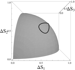
Figure 1: The top view of the parametrical plot ($\Delta S_{1}(t),\Delta S_{2}(t),\Delta S_{3}(t)$) of the closed space curve (22) on the positive 1/8 part of the sphere for a spin 1 with the parameters of the circularly polarised field $\omega=H=1$,   $h=2$.

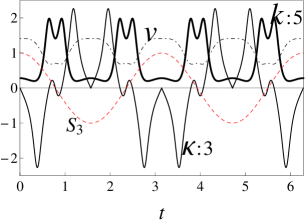
Figure 2: Dynamics of $S_{3}$, curvature $k$, torsion of curve $\kappa$, velocity modulus of an apex $V$ for a spin 1 with the parameters as in Fig. 1.

The real and non-negative eigenvalues of the $3\times 3$ covariance matrix

$$\mathrm{Cov}(S_{i},S_{k})=\frac{1}{2}\mathrm{Tr\,}\left[\rho\,\left(C_{i}C_{k}+C_{k}C_{i}\right)\right]-\mathrm{Tr\,}\left[\rho\,C_{i}\right]\mathrm{Tr\,}\left[\rho\,C_{k}\right]$$ (21)

equal $\lambda_{1}=\lambda_{2}=\frac{S}{2},\lambda_{3}=0$ and the invariants of the tensor are $\lambda_{1}+\lambda_{2},\lambda_{1}\lambda_{2},\lambda_{3}$.
Hence, the sum of the variances Maccone and Pati (2014); Chen and Fei (2015) of the spin components $S_{i}$ in the magnetic resonance in the circularly polarized magnetic field is conserved for any $t$ during the evolution:

$$(\Delta S_{1})^{2}+(\Delta S_{2})^{2}+(\Delta S_{3})^{2}=S,$$ (22)

where $(\Delta S_{1},\Delta S_{2},\Delta S_{3})=1/2\sqrt{S/2}(\sqrt{3+\cos 2ht+2\sin^{2}ht\cos 2\omega t},\\ \sqrt{3+\cos 2ht-2\sin^{2}ht\cos 2\omega t},2\left|\sin ht\right|).$ In the consistent field the relation (22) is fulfilled only for a qubit and a qutrit.
Due to $\Delta S_{1}(t)\geq 0,\Delta S_{2}(t)\geq 0,\Delta S_{3}(t)\geq 0$ and quantum restriction (22), the curve lies on 1/8 part of the sphere. This curve is the closed one with period $T_{c}=2\pi m/h=\pi l/\omega$, where $m,l$ are integers. The oriented spherical curve is characterized by the curvature $k$, torsion of the curve $\kappa$, apex speed $V$, and length of the path $s$ Aminov (1987); Ivanchenko (2013). In Fig. 2 it is shown that the speed $V$ is minimum, when $S_{3}$ and $\kappa$ change a sign and $k$ has a local minimum. $S_{3}$ is extreme, when $V$ is maximal, $k$ is minimum, $\kappa$ has a local maximum/local minimum. The quantitative characteristic of the curve at the coordinates $\Delta S_{1},\Delta S_{2},\Delta S_{3}$ in Fig. 1 represents in details the resonant evolution in Fig. 2.
It is possible to apply a known bilateral inequality (between the harmonic, geometrical and arithmetic averages) to the estimation of the product of two $\Delta S_{i}\Delta S_{k},(i\neq k=1,2,3)$ and three standard deviations $\Delta S_{1}\Delta S_{2}\Delta S_{3}$. The dynamics of the spin standard deviations and their products is presented in Fig. 1,3.

Figure 3: Dependence of the products of two and three standard deviations on time for a spin 1 with the parameters as in Fig. 1. Dashed and dot-dashed lines accordingly specify the arithmetic average and the harmonic one; black thick lines show the analytic solution.

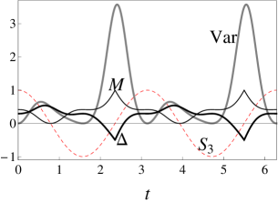
Figure 4: Dynamics of $S_{3},\,M(S_{1}:S_{2}),\,\Delta(S_{1}|S_{2}),\,\mathrm{Var\,}(S_{1}|S_{2})$ for a spin 1 with the parameters as in Fig. 1.

In Fig. 3 the plots of the harmonious, geometrical and arithmetic averages are presented. As it can be seen in Fig. 3 for both $\Delta S_{1}\Delta S_{2}$ and $\Delta S_{1}\Delta S_{3},\Delta S_{2}\Delta S_{3}$ the inequalities practically transform locally into the equalities when the equation (22) represents the closed curve on the sphere.
In terms of the standard spin deviations and new notions Sazim et al. (2017): it is possible to describe the dynamics of the magnetic resonance with help of the mutual uncertainty ($M$) $M(S_{i}:S_{k})=\Delta S_{i}+\Delta S_{k}-\Delta(S_{i}+S_{k})$, the conditional uncertainty ($\Delta$) $\Delta(S_{i}|S_{k})=\Delta(S_{i}+S_{k})-\Delta S_{k}$ and the conditional variance (Var) $\mathrm{Var\,}(S_{i}|S_{k})=\mathrm{Var\,}(S_{i}+S_{k})-\mathrm{Var\,}S_{k}$.
From Fig. 2,4,5 it is seen that M, $\Delta$, Var are extreme when $S_{3}$ changes sign. For the spin $S\geq 1$ we obtain $M\geq 0$, $\mathrm{Var\,}\geq 0$ and $\Delta$ is sign-changing. The conditional variance equals zero in the exact resonance ($S_{3}=-1$). These new characteristics specify the description of the magnetic resonance.

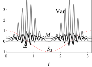
Figure 5: The same as in Fig. 4 with the parameters $\omega=H=20$,  $h=2$.

The description of the magnetic resonance both in geometrical terms of Figs. 1,2 and in terms of conditional uncertainty and variance Figs. 4,5 mutually complement each other.

IV Conclusion

At resonance in the circularly polarization field the Bloch sphere radius is limited by value $\sqrt{3}$ when $S\rightarrow\infty$. The Fubini-Study measure in the finite-dimensional spin space is specified. The universal length value is found both for $S=1/2,1$ in the coordinated magnetic field and for any $S$ in the circularly polarization field. For any spin the bottom bounds QSLs are found. With the spin growth the transition time between levels decreases. The minimal time goes to zero at $H\ll h$. The dynamics of the spin standard deviations has been presented. An experimental confirmation of our results can be implemented at $H\gg h$ using a NMR setup Miller et al. (2001); Ma et al. (2017).

References

- Ivanchenko (2005a) E. A. Ivanchenko, Physica B 358, 308 (2005a).
- Ivanchenko (2005b) E. A. Ivanchenko, Low Temp. Phys. 31, 577 (2005b).
- Abramovitz and Stegun (1968) M. Abramovitz and I. A. Stegun, Handbook of Mathematical Functions, edited by I. A. Stegun (Dover, New York, 1968) p. 832.
- Rabi (1937) I. I. Rabi, Phys. Rev. 51, 652 (1937).
- Bambini and Berman (1981) A. Bambini and P. R. Berman, Phys. Rev. A 23, 2496 (1981).
- Bloch and Siegert (1940) F. Bloch and A. Siegert, Phys. Rev. 57, 522 (1940).
- Ivanchenko (2013) E. A. Ivanchenko, arXiv:1311.2537v2 [quant-ph] 11 Nov (2013).
- Mandelstam and Tamm (1945) L. Mandelstam and I. Tamm, J. Phys. USSR 9, 249 (1945).
- Anandan and Aharonov (1990) J. Anandan and Y. Aharonov, Phys. Rev. Lett. 65, 1697 (1990).
- Vaidman (1992) L. Vaidman, Am. J. Phys. 60, 182 (1992).
- Margolus and Levitin (1998) N. Margolus and L. B. Levitin, Physica D 120, 188 (1998).
- Levitin and Toffoli (2009) L. B. Levitin and T. Toffoli, Phys. Rev. Lett. 103, 160502 (2009).
- Pires et al. (2016) D. P. Pires, M. Cianciaruso, L. C. Celeri, G. Adesso, and D. O. Soares-Pinto, Phys. Rev. X 6, 021031 (2016).
- Molotkov and Nazin (1996) S. N. Molotkov and S. S. Nazin, JETP Lett. 63, 924 (1996).
- Caneva et al. (2009) T. Caneva, M. Murphy, T. Calarco, R. Fazio, S. Montangero, V. Giovannetti, and G. E. Santoro, Phys. Rev. Lett. 103, 240501 (2009).
- Zhang et al. (2015) T.-M. Zhang, R.-B. Wu, F.-H. Zhang, T.-J. Tarn, and G.-L. Long, IEEE TRANSACTIONS ON CONTROL SYSTEMS TECHNOLOGY 23, 2018 (2015).
- Markov (2014) I. L. Markov, Nature 512, 147 (2014).
- Heaney and Vedral (2009) L. Heaney and V. Vedral, Phys. Rev. Lett. 103, 200502 (2009).
- Deffner and Lutz (2010) S. Deffner and E. Lutz, Phys. Rev. Lett. 105, 170 (2010).
- Chin et al. (2012) A. W. Chin, S. F. Huelga, and M. B. Plenio, Phys. Rev. Lett. 109, 233601 (2012).
- Ivanchenko (2009) E. A. Ivanchenko, J. Math. Phys. 50, 042704 (2009).
- Ivanchenko (2012) E. A. Ivanchenko, Int. J. Quant. Inf. 10, 1250068 (2012).
- Feynman et al. (1957) R. P. Feynman, J. F. L. Vernon, and R. W. Hellwarth, Journal of applied physics 28, 49 (1957).
- Aminov (1987) Y. A. Aminov, Differential geometry and topology of curves, edited by Mistshenko (Nauka, Moskow, 1987) p. 160.
- Stu (1985) in The mathematical encyclopaedia, Vol. 5, edited by I. M. Vinogradov (The Soviet encyclopaedia, Moskow, 1985) p. 1 247.
- Dodonov et al. (1999) V. V. Dodonov, O. V. Man’ko, V. I. Man’ko, and A. Wuensche, Phys.Scripta 59, 81 (1999).
- Deffner and Lutz (2013) S. Deffner and E. Lutz, Journal of Physics A: Mathematical and Theoretical 46, 335302 (2013).
- Hegerfeldt (2014) G. C. Hegerfeldt, Phys. Rev. A 90, 032110 (2014).
- Maccone and Pati (2014) L. Maccone and A. K. Pati, Phys. Rev. Lett. 113, 260401 (2014).
- Chen and Fei (2015) B. Chen and S. M. Fei, Scientific Reports 5, 14238 (2015).
- Sazim et al. (2017) S. Sazim, S. Adhikari, A. K. Pati, and P. Agrawal, arXiv:1702.07576v2 [quant-ph] (2017).
- Miller et al. (2001) J. B. Miller, B. H. Suits, and A. N. Garroway, Journal of Mag. resonance 151, 228 (2001).
- Ma et al. (2017) W. Ma, B. Chen, Y. Liu, M. Wang, X. Ye, F. Kong, F. Shi, S.-M. Fei, and J. Du, Phys. Rev. A 95, 042334 (2017).