A Model of Controlled Growth

Abstract

We consider a free boundary problem for a system of PDEs, modeling the growth of a biological tissue. A morphogen, controlling volume growth, is produced by specific cells and then diffused and absorbed throughout the domain. The geometric shape of the growing tissue is determined by the instantaneous minimization of an elastic deformation energy, subject to a constraint on the volumetric growth. For an initial domain with ${\cal C}^{2,\alpha}$ boundary, our main result establishes the local existence and uniqueness of a classical solution, up to a rigid motion.

1 Introduction

Aim of this paper is to analyze a system of PDEs on a variable domain, describing the growth of a biological tissue. Motivated by [2, 3, 4], we consider a living tissue containing some “signaling cells”, which produce morphogen (i.e., a growth-inducing chemical). This morphogen diffuses throughout the tissue and is partially absorbed. A “chemical gradient” is thus created: the concentration of morphogen is not uniform, being larger in regions closer to the signaling cells. In turn, this variable concentration determines a different volumetric growth in different parts of the living tissue. This can provide a mechanism for controlling the growth of the domain toward a desired shape.

As customary, we describe biological growth in terms of a vector field ${\bf v}(\cdot)$, determining the motion of single cells within the tissue. Calling $u(\cdot)$ the concentration of morphogen, the constraint on volumetric growth is expressed by

$$\hbox{div}\,{\bf v}~{}=~{}g(u)\,,$$ (1.1)

where $g:{\mathbb{R}}\to{\mathbb{R}}_{+}$ is a (possibly nonlinear) response function, satisfying $g(0)=0$. At any given time $t$, the vector field ${\bf v}$ is then determined (up to a rigid motion) by the requirement that it minimizes a deformation energy, subject to the constraint (1.1). The model is closed by the assumption that signaling cells are passively transported within the tissue.

Calling $\Omega(t)$ the region occupied by the tissue at time $t$, and $w(t,\cdot)$ the concentration of signaling cells, we prove that the above model yields a well posed initial value problem. More precisely, our main theorems show that, if the initial domain $\Omega(0)=\Omega_{0}$ has ${\cal C}^{2,\alpha}$ boundary and if the initial concentration $w(0,\cdot)$ lies in the Hölder space ${\cal C}^{0,\alpha}(\Omega_{0})$ for some $0<\alpha<1$, then the system of evolution equations determining the growing domain has a classical solution, locally in time. Moreover, this solution is unique up to rigid motions, and preserves the regularity of the initial data.

A wide literature is currently available on free boundary problems modeling set growth, see for example [5, 7, 8, 13, 19, 20]. A major goal of these studies has been the mathematical description of tumor growth [6, 9, 10, 11, 14, 15]. Compared with earlier works, our model has various new features. On one hand, it contains a transport equation for the density of morphogen-producing cells. By varying the location and concentration of these cells, one can study how different shapes are produced. Another fundamental difference is that in our model the velocity field ${\bf v}$ is found as the minimizer of an elastic deformation energy involving the $L^{2}$ norm of the symmetric gradient of ${\bf v}$. On the other hand, in free boundary problems modeling flow in porous media one minimizes the $L^{2}$ norm of the velocity field ${\bf v}$ itself (with suitable constraints). As a consequence, while the solutions in [6, 9, 10, 11, 14, 15] are unique, the solutions that we presently construct are uniquely determined only up to rigid motions.

The remainder of this paper is organized as follows. In Section 2 we introduce the basic model and collect the main notation. Section 3 contains some geometric lemmas on the representation of a family of sets with sufficiently smooth boundary.

The heart of the matter is worked out in Section 4, where we construct approximate solutions by a time discretization algorithm. At each time step, the density $u(\cdot)$ of morphogen satisfies a linear elliptic equation accounting for production, diffusion, and adsorption. Existence and regularity of solutions follow from standard theory [16]. In turn, the existence of a vector field ${\bf v}(\cdot)$ satisfying the divergence constraint (1.1) and minimizing a suitable elastic deformation energy is proved relying on Korn’s inequality. A careful analysis shows that the system of equations determining this constrained minimizer is elliptic in the sense of Agmon, Douglis, and Nirenberg. Thanks to the Schauder type estimates proved in [1], we thus obtain the crucial a-priori bound on the norm $\|{\bf v}\|_{{\cal C}^{2,\alpha}}$. Finally, the density $w(\cdot)$ of signaling cells is updated in terms of a linear transport equation with ${\cal C}^{2,\alpha}$ coefficients, providing an estimate on how the norm $\|w\|_{{\cal C}^{0,\alpha}}$ grows in time. Section 5 contains some additional estimates, showing that our approximate solutions depend continuously on the initial data.

In Section 6 we state and prove our first main result, on the existence of classical solutions, locally in time. The uniqueness of these solutions, up to rigid motions, is then proved in Section 7. Two simple examples, where the growing domain $\Omega(t)$ can be explicitly computed, are discussed in Section 8.

The last two sections contain some supplementary material. In Section 9 we reformulate the problem using Lagrangian coordinates. Namely, we show that the growth of the living tissue can be described by an evolution equation for the coefficients of a Riemann metric tensor on a fixed domain. Finally, an extension of our basic model is proposed in Section 10, where we derive a set of equations describing the growth of a 2-dimensional surface embedded in ${\mathbb{R}}^{3}$, regarded as a thin elastic shell.

2 The basic model

Let $\Omega(t)\subset{\mathbb{R}}^{d}$ be the region occupied by a living tissue at time $t$, in a space of dimension $d$. Cases $d=2$ or $d=3$ are the most relevant, however we formulate and prove our results in the general case of arbitrary dimension.

Assume that a morphogen is produced by cells located within the tissue. Denote by $w(t,x)$ the density of these cells at time $t$ and at a point $x\in\Omega(t)$. Calling $u=u(t,x)$ the concentration of morphogen, we shall assume that $u$ satisfies a linear diffusion-adsorption equation with Neumann boundary conditions:

$$\left\{\begin{array}[]{ll}u_{t}=\Delta u-u+w&x\in\Omega(t),\cr\langle\nabla u,{\bf n}\rangle=0&x\in\partial\Omega(t).\end{array}\right.$$

Since the time scale of chemical diffusion is much shorter than the time scale of tissue growth, at any given time $t$ the solution of the above problem will be very close to an equilibrium, described by the elliptic equation

$$\left\{\begin{array}[]{ll}\Delta u-u+w=0&x\in\Omega(t),\cr\langle\nabla u,{\bf n}\rangle=0&x\in\partial\Omega(t).\end{array}\right.$$ (2.1)

We observe that, for every $w\in L^{2}(\Omega(t))$, the solution $u$ of (2.1) provides the unique minimizer of a quadratic functional over the space $W^{1,2}(\Omega(t))$. Namely, it solves the problem

$$\hbox{minimize:}\quad J(u)~{}\doteq~{}\int_{\Omega(t)}\Big{(}{|\nabla u|^{2}\over 2}+{u^{2}\over 2}-wu\Big{)}~{}\mbox{d}x.$$ (M)

Next, we need an equation describing motion of cells within the tissue. This is determined by the expansion caused by volume growth. Call ${\bf v}={\bf v}(t,x)$ the velocity of the cell located at $x\in\Omega(t)$ at time $t$. In our model, at each time $t$, the vector field ${\bf v}(t,\cdot)$ is determined as the solution to the constrained minimization problem

$$\hbox{minimize:}\quad E({\bf v})~{}\doteq~{}{1\over 2}\int_{\Omega(t)}|\hbox{sym}\,\nabla{\bf v}|^{2}~{}\mbox{d}x\qquad\hbox{subject to:}\quad\hbox{div}\,{\bf v}~{}=~{}g(u)\,.$$ (E)

Notice that $E({\bf v})$ can be regarded as the elastic energy of an infinitesimal deformation (displacement). Throughout the paper, we assume that the function $g:{\mathbb{R}}\to[0,\infty)$ satisfies

$$g\in{\cal C}^{3}({\mathbb{R}}),\qquad g(0)=0,\qquad g^{\prime},~{}g^{\prime\prime},~{}g^{\prime\prime\prime}\mbox{ are uniformly bounded.}$$ (2.2)

Finally, we assume that the morphogen-producing cells are passively transported within the tissue. The transport equation below is supplemented by assigning an initial distribution of hormone-producing cells on the initial domain:

$$\left\{\begin{array}[]{ll}w_{t}+\hbox{div}\,(w{\bf v})=0&\qquad\qquad x\in\Omega(t),\cr w(0,x)=w_{0}(x)&\qquad\qquad x\in\Omega(0)=\Omega_{0}.\end{array}\right.$$ (H)

Notice that, as soon as the velocity field ${\bf v}$ is known, we can recover $\Omega(t)$ as the set reached at time $t$ by trajectories starting in $\Omega_{0}$. More precisely:

$$\Omega(t)=\bigg{\{}x(t)\,;\quad x(0)=x_{0}\in\Omega_{0}~{}\mbox{ and }~{}x^{\prime}(s)={\bf v}(s,x(s))~{}~{}\hbox{for all}~{}s\in[0,t]\bigg{\}}.$$ (G)

Summarizing, we have:

• The linear elliptic equation (2.1), describing the concentration of morphogen $u$ over the set $\Omega(t)$, at each time $t\geq 0$. For a given source term $w(t,\cdot)$, its solution $u(t,\cdot)$ provides the unique minimizer in (M).

• A constrained minimization problem (E), determining the velocity field ${\bf v}(t,\cdot)$ at each given time $t$, up to a rigid motion: translation + rotation.

• The linear transport equation (H), determining how the concentration of morphogen-producing cells evolves in time.

• The formula (G), describing the growth of the domain $\Omega(t)$.

The main goal of our analysis is to prove that, given an initial set $\Omega_{0}$ and an initial density $w_{0}(x)$ for $x\in\Omega_{0}$, the equations (M-E-H-G) determine a unique evolution (at least locally in time), up to a rigid motion that does not affect the shape of the growing domain.

2.1 Notation

Throughout this paper, by ^′ or $\frac{{\rm d}}{{\rm d}t}$ we denote a derivative w.r.t. time $t$, while $\nabla$ is the gradient w.r.t. the space variable $x=(x_{1},\ldots,x_{d})$.

Given a bounded, open, simply connected set $\Omega\subset{\mathbb{R}}^{d}$, its boundary is denoted by $\Sigma=\partial\Omega$, and its Lebesgue measure by $|\Omega|$. We write ${\bf n}$ for the outer unit normal vector to $\Omega$ at boundary points, while $T_{P}(\partial\Omega)$ is the space of tangent vectors to the boundary $\partial\Omega$ at the point $P$. The average value of a function $f$ on $\Omega$ is denoted by

$$-\!\!\!\!\!\!\int_{\Omega}f~{}\mbox{d}x\doteq\frac{1}{|\Omega|}\int_{\Omega}f~{}\mbox{d}x.$$

For any integer $k\geq 0$ and $\alpha\in(0,1)$, by ${\cal C}^{k,\alpha}(\Omega)$ we mean the space of bounded continuous functions whose derivatives up to order $k$ are Hölder continuous on $\Omega$, with the exponent $\alpha$. This is a Banach space with the norm:

$$\|u\|_{{\cal C}^{k,\alpha}(\Omega)}~{}\doteq~{}\sum_{|\nu|\leq k}~{}\sup_{x\in\Omega}|\nabla^{\nu}u(x)|+\sum_{|\nu|=k}~{}\sup_{x,y\in\Omega,\,x\not=y}~{}{|\nabla^{\nu}u(x)-\nabla^{\nu}u(y)|\over|x-y|^{\alpha}}\,.$$

Since every Hölder continuous function $u$ as above admits a unique extension to the closure $\overline{\Omega}$, we observe that the spaces ${\cal C}^{k,\alpha}(\Omega)$ and ${\cal C}^{k,\alpha}(\overline{\Omega})$ can be identified.

Given a $d\times d$ matrix $A=[A_{ij}]_{i,j=1\ldots d}$, we denote by $A^{T}=[A_{ji}]$ its transpose, and we set:

$$\hbox{sym}\,A~{}\doteq~{}{A+A^{T}\over 2}\,,\qquad\hbox{\rm skew}\,A~{}\doteq~{}{A-A^{T}\over 2}\,,$$

$$\langle A:B\rangle~{}\doteq~{}\mbox{trace}(A^{T}B)\,,\qquad|A|^{2}~{}\doteq~{}\langle A:A\rangle=\sum_{i,j=1}^{d}A_{ij}^{2}.$$

The space of $d\times d$ skew-symmetric matrices is $so(d)$, and $I$ is the $d\times d$ identity matrix.

3 Some geometric lemmas

We say that $\Omega$ satisfies the uniform inner and outer sphere condition when there exists $\rho>0$ such that, for every boundary point $x\in\Sigma$, we can find closed balls $B^{in}$ and $B^{out}$ of radii $R_{{in}}(x),R_{{out}}(x)\geq 2\rho$ satisfying $B^{in}\subset\overline{\Omega}$, $B^{in}\cap\Sigma=\{x\}$ and $B^{out}\cap\overline{\Omega}=\{x\}$. Define the signed distance function:

$$\delta(x)~{}\doteq~{}\left\{\begin{array}[]{cl}~{}{\rm dist}(x,\Sigma)&~{}~{}x\notin\Omega\cr-{\rm dist}(x,\Sigma)&~{}~{}x\in\Omega.\end{array}\right.$$

If $\Omega$ is smooth (i.e., it has a smooth boundary), then $\delta(\cdot)$ is also smooth, when restricted to the open set

$$V_{\rho}~{}\doteq~{}\{x;~{}~{}{\rm dist}(x,\Sigma)<\rho\}.$$

Moreover, for every $x\in V_{\rho}$ there exists a unique point $\pi(x)\in\Sigma$ with $|\pi(x)-x|={\rm dist}(x,\Sigma).$

Every continuous map $\varphi:\Sigma\to(-\rho,\rho)$ determines then a bounded open set (see Fig. 1):

$$\Omega^{\varphi}=\bigl{\{}x\in{\mathbb{R}}^{d};~{}~{}\delta(x)<\varphi(\pi(x))\bigr{\}}\quad\mbox{with}\quad\partial\Omega^{\varphi}=\bigl{\{}y+\varphi(y)\,{\bf n}(y);~{}~{}y\in\Sigma\bigr{\}}.$$ (3.1)

To measure the Hölder regularity of $\varphi$, we extend it to $V_{\rho}$ by $\varphi(x)\doteq\varphi(\pi(x))$, and set:

$$\|\varphi\|_{\mathcal{C}^{k,\alpha}}~{}\doteq~{}\|\varphi\|_{\mathcal{C}^{k,\alpha}(V_{\rho})}.$$ (3.2)

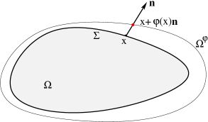
Figure 1: The set $\Omega^{\varphi}$ in (3.1), described in terms of the function $\varphi:\Sigma\to{\mathbb{R}}$.

By definition, $\Sigma\in{\cal C}^{k,\alpha}$ if the following holds. For every $x\in\Sigma$ there exists an open ball $B(x,r)$ and a homeomorphism $h:B(x,r)\to B(0,1)\subset{\mathbb{R}}^{d}$ such that :

• The map $h$ as well as its inverse $h^{-1}$ are ${\cal C}^{k,\alpha}$ regular.

• $h\big{(}B(x,r)\cap\Omega\big{)}=B(0,1)\cap\bigl{\{}x\in{\mathbb{R}}^{d};~{}x_{1}>0\bigr{\}}.$

Lemma 3.1.

Let $\Omega\subset{\mathbb{R}}^{d}$ be an open, bounded, simply connected and smooth set, satisfying the uniform inner and outer sphere condition with radius $2\rho>0$. Then, for every $\kappa>0$ there exists a constant $M$ such that the following holds. If $\varphi:\Sigma\to(-\frac{\rho}{2},\frac{\rho}{2})$ satisfies $\|\varphi\|_{{\cal C}^{2,\alpha}}\leq\kappa$, then there exists a homeomorphism $\Lambda:\Omega\to\Omega^{\varphi}$ satisfying the bounds:

$$\|\Lambda\|_{{\cal C}^{2,\alpha}(\Omega)}\leq M,\qquad\quad\|\Lambda^{-1}\|_{{\cal C}^{2,\alpha}(\Omega^{\varphi})}\leq M.$$ (3.3)

Proof. 1. Let $\sigma:{\mathbb{R}}\to{\mathbb{R}}$ be a ${\cal C}^{\infty}$ function such that $\sigma(s)=0$ for $s\leq-{\rho}$, and $\sigma(x)=1$ for $s\geq 0$, and moreover:

$$0\leq\sigma^{\prime}(s)\leq\frac{3}{2\rho}\quad~{}\hbox{for all}\quad s\in{\mathbb{R}}.$$ (3.4)

The homeomorphism $\Lambda:\Omega\to\Omega^{\varphi}$ is defined by setting:

$$\Lambda(x)=\left\{\begin{array}[]{cl}x&\hbox{if}\quad~{}~{}\delta(x)\leq-\rho\\ x+\sigma(\delta(x))\varphi(x){\bf n}(\pi(x))&\hbox{if}\quad-\rho<\delta(x)<0.\end{array}\right.$$

It is easily seen that $\Lambda$ maps $\Omega$ onto $\Omega^{\varphi}$. Since $\Lambda$ coincides with identity on the set where $\delta(x)\leq-\rho$, to estimate the ${\cal C}^{2,\alpha}$ norm of $\Lambda$ it suffices to study what happens when $-\rho<\delta(x)<0$. On this latter set, the functions $\delta(x)$, $\sigma(\delta(x))$, ${\bf n}(\pi(x))$ have uniformly bounded derivatives up to any order. By the definition of $\Lambda$ we thus get the estimate:

$$\|\Lambda\|_{{\cal C}^{2,\alpha}(\Omega)}\leq C\big{(}1+\|\varphi\|_{{\cal C}^{2,\alpha}}\big{)},$$

for a suitable constant $C$ depending only on $\Sigma$.

2. In order to obtain a similar estimate for $\Lambda^{-1}$, it is enough to check that $\det\nabla\Lambda$ has uniformly bounded inverse on $\Omega$. Indeed, in this case, the ${\cal C}^{2,\alpha}$ norm of $\Lambda^{-1}$ will be bounded by a polynomial in $\|\Lambda\|_{{\cal C}^{2,\alpha}(\Omega)}$ whose order and coefficients depend only on $\Omega$ and $d$.

On the set where $\delta(x)\leq-\rho$, we have $\det\nabla\Lambda=1$. Let now $-\rho<\delta(x)<0$, and let $y=\pi(x)\in\Sigma$. Let $U\subset\Sigma$ be a relatively open neighborhood of $y$, with coordinates $(x_{2},\ldots,x_{d})$. Then the map $x\mapsto(\delta(x),x_{2},\ldots,x_{d})$ provides a chart of the inverse image $\pi^{-1}(U)$. In these coordinates, $\Lambda$ has the form:

$$\widetilde{\Lambda}(x_{1},\ldots,x_{d})~{}=~{}\big{(}x_{1}+\sigma(x_{1})\varphi(x),x_{2},\ldots,x_{d}\big{)}.$$

In view of (3.4) and the fact that $\varphi$ is independent of $x_{1}$, we thus conclude:

$$\det\nabla\widetilde{\Lambda}(x)~{}=~{}1+\sigma^{\prime}(x_{1})\phi(x)~{}\geq~{}1-\frac{3}{2\rho}\frac{\rho}{2}~{}=~{}\frac{1}{4}.$$

The estimate (3.3) now follows by covering the compact surface $\Sigma$ with finitely many coordinate charts and by noting that, on each chart, $\det\nabla\Lambda$ is uniformly comparable with $\det\nabla\widetilde{\Lambda}$. MM     

Lemma 3.2.

Let $\Omega_{0}\subset{\mathbb{R}}^{d}$ be an open, bounded and simply connected set with ${\cal C}^{2,\alpha}$ boundary $\Sigma_{0}$, satisfying the uniform inner and outer sphere condition with radius $3\rho>0$. Then, for any $\varepsilon_{0}>0$, there exists an open, bounded and simply connected set $\Omega$ with ${\cal C}^{\infty}$ boundary $\Sigma$, satisfying the uniform inner and outer sphere condition with radius $2\rho$, and such that $\Omega_{0}=\Omega^{\varphi}$ as in (3.1) for some function $\varphi\in{\cal C}^{2,\alpha}(\Sigma)$ with:

$$|\varphi(x)|<\varepsilon_{0}\quad\mbox{for all}\quad x\in\Sigma.$$ (3.5)

Proof. 1. Let $\delta_{0}$ be the signed distance function from $\Sigma_{0}$. By assumption, $\delta_{0}$ is ${\cal C}^{2}$ on the open neighborhood $V_{0,3\rho}$ of $\Sigma_{0}$ with radius $3\rho$. We now consider the mollification $\delta_{\varepsilon}=\delta_{0}*J_{\varepsilon}$ with a standard mollifier $J_{\varepsilon}$ in ${\mathbb{R}}^{d}$. It is not restrictive to assume that $\varepsilon\ll\varepsilon_{0}\ll\rho$ and that

$$\|\delta_{\varepsilon}-\delta_{0}\|_{{\cal C}^{2,\alpha}(V_{0,3\rho-\varepsilon_{0}})}\leq C\varepsilon.$$ (3.6)

We claim that the set

$$\Omega=\Omega_{\varepsilon}~{}\doteq~{}\{x\in{\mathbb{R}}^{d};~{}~{}\delta_{\varepsilon}(x)<0\}$$

satisfies the conclusions of the lemma, provided that $\varepsilon>0$ is chosen sufficiently small. Since $|\nabla\delta_{0}|=1$ in $V_{0,3\delta}$, we note that:

$$|\nabla\delta_{\varepsilon}(x)|\geq 1-{\varepsilon_{0}\over 2}\quad\hbox{for all}~{}x\in V_{0,3\rho},\qquad|\delta_{\varepsilon}(x)|\leq{\varepsilon_{0}\over 2}\quad\hbox{for all}~{}x\in\Sigma_{0}.$$

Now fix $x\in\Sigma_{0}$. By the above estimates and since $\delta_{0}\in\mathcal{C}^{2}$, we can find $y\in V_{0,\rho}$ such that

$$\delta_{\varepsilon}(y)=0\qquad\hbox{and}\qquad|y-x|\leq{\varepsilon_{0}\over 2}\left(1-{\varepsilon_{0}\over 2}\right)^{-1}<\varepsilon_{0}.$$

Consequently, every point $x\in\Sigma_{0}$ is at a distance less than $\varepsilon_{0}$ from some $y\in\Sigma_{\varepsilon}=\partial\Omega_{\varepsilon}$. We conclude that the smooth set $\Omega=\Omega_{\varepsilon}$ indeed satisfies $\Omega^{\varphi}=\Omega_{0}$ and the uniquely determined function $\varphi$, given as the signed distance from $\Sigma$, obeys (3.5) and it is ${\cal C}^{2,\alpha}$ regular.

2. We now check that $\Omega=\Omega_{\varepsilon}$ satisfies the uniform inner and outer sphere condition with radius $2\rho$. Fix any point $P\in\Sigma_{0}$. On a neighborhood of $P$ we introduce an orthonormal frame of coordinates $(y_{1},\ldots,y_{d})=(y_{1},\tilde{y})$ as in Fig. 2, where the $y_{1}$-axis is orthogonal to the surface $\Sigma_{0}$ at $P$. In these local coordinates, the surfaces $\Sigma_{0}$, $\Sigma_{\varepsilon}$ have the representations:

$$\Sigma_{0}=\{(y_{1},\tilde{y});~{}~{}y_{1}=\psi_{0}(\tilde{y})\bigr{\}},\qquad\Sigma_{\varepsilon}=\{(y_{1},\tilde{y});~{}~{}y_{1}=\psi_{\varepsilon}(\tilde{y})\bigr{\}},$$

with the variable $\tilde{y}$ ranging in some neighborhood of the origin $U\subset{\mathbb{R}}^{d-1}$.

By construction we have $\frac{\partial\delta_{0}}{\partial y_{1}}(P)=1$. Hence, by possibly shrinking the neighborhood $U$, we can assume $\frac{\partial\delta_{0}}{\partial y_{1}}(\tilde{y})\geq\frac{1}{2}$ for every $\tilde{y}\in U$. By (3.6) we thus have $\|\psi_{\varepsilon}-\psi_{0}\|_{{\cal C}^{0}(U)}\leq C\varepsilon$ and the implicit function theorem further implies the convergence

$$\|\psi_{\varepsilon}-\psi_{0}\|_{{\cal C}^{2}(U)}~{}\to~{}0\qquad\qquad\hbox{as}\quad\varepsilon\to 0\,.$$ (3.7)

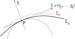
Figure 2: Estimating the radius of curvature of the boundary $\Sigma_{\varepsilon}=\partial\Omega_{\varepsilon}$

We now recall that the maximal curvature $\chi(\tilde{y})$ of the graph of a function $\psi:{\mathbb{R}}^{d-1}\to{\mathbb{R}}$ at a point $\tilde{y}$, equals the maximum of the absolute values of the principal curvatures, i.e. the maximum of the absolute values of the eigenvalues of the second fundamental form $\Pi=(\nabla\psi)^{T}\nabla\mathbf{n}$. Since the second fundamental forms of $\Sigma_{0}$ and $\Sigma_{\varepsilon}$ satisfy: $\|\Pi_{\varepsilon}-\Pi_{0}\|_{{\cal C}^{0}(U)}\to 0$ as $\varepsilon\to 0$ in virtue of (3.7), and since for every $\tilde{y}\in U$ the assumption of the lemma gives: $\chi_{0}(\tilde{y})\leq\frac{1}{3\rho}$, it indeed follows that $\chi_{\varepsilon}(\tilde{y})\leq\frac{1}{2\rho}$ for small $\varepsilon>0$.

In turn, this yields an a-priori bound on the inner and outer curvature radii:

$$\min\bigl{\{}R_{in}(\psi_{\varepsilon}(\tilde{y}),\tilde{y}),~{}R_{out}(\psi_{\varepsilon}(\tilde{y}),\tilde{y})\bigr{\}}~{}=~{}{1\over\chi_{\varepsilon}(\tilde{y})}~{}\geq~{}2\rho.$$

By covering the compact surface $\Sigma_{0}$ with neighborhoods of finitely many points $P_{1},\ldots,P_{\nu}$, and choosing $\varepsilon=\min\{\varepsilon_{1},\ldots,\varepsilon_{\nu}\}$, the proof is achieved. MM     

4 Regularity estimates

Given the initial data $w_{0}$ in (H), a local solution to the system of equations (M-E-H-G) will be constructed as a limit of approximations, obtained by discretizing time.

Fix a time step $\epsilon>0$ and let $t_{k}=k\epsilon$. Assume that at time $t_{k}$ we are given the set $\Omega_{k}=\Omega(t_{k})$ and the scalar nonnegative function $w_{k}=w(t_{k},\cdot)$ on $\Omega_{k}$. Successive $\Omega_{k+1}=\Omega(t_{k+1})$ and $w_{k+1}=w(t_{k+1},\cdot)$ on $\Omega_{k+1}$ are obtained by the application of the four steps below.

Step 1.

Determine the density $u_{k}:\Omega_{k}\to{\mathbb{R}}$ by minimizing (M) with $w=w_{k}$. This implies that $u_{k}$ is the solution to the elliptic problem (2.1).

Step 2.

Determine the velocity field ${\bf v}_{k}:\Omega_{k}\to{\mathbb{R}}^{d}$ by solving the minimization problem (E) on $\Omega_{k}$ subject to the current constraint $\hbox{div}\,{\bf v}_{k}=g(u_{k})$. The minimum is defined up to a rigid motion and we can single out a unique ${\bf v}_{k}$ by requiring that

$$-\!\!\!\!\!\!\int_{\Omega_{k}}{\bf v}_{k}~{}\mbox{d}x=0\,,\qquad\qquad\hbox{\rm skew}\,\displaystyle{-\!\!\!\!\!\!\int_{\Omega_{k}}\nabla{\bf v}_{k}~{}\mbox{d}x=0.}$$ (4.1)

Step 3.

Define the domain $\Omega_{k+1}$ by an approximation of (G):

$$\Omega_{k+1}~{}\doteq~{}\bigl{\{}x+\epsilon{\bf v}_{k}(x);~{}x\in\Omega_{k}\bigr{\}}.$$ (4.2)

Step 4.

On the set $\Omega_{k+1}$, define the density $w_{k+1}$ implicitly by setting

$$w_{k+1}(x+\epsilon{\bf v}_{k}(x))~{}\doteq~{}{w_{k}(x)\over\det(I+\epsilon\nabla{\bf v}_{k}(x))}\,.$$ (4.3)

Notice that (4.3) is motivated by mass conservation: $w_{k+1}$ is the push-forward of the density $w_{k}$ through the map $x\mapsto x+\epsilon{\bf v}_{k}(x)$. The motivation for (4.3) in the continuous framework is given in Lemma 4.5.

Throughout the following, we assume that the initial domain $\Omega_{0}\subset{\mathbb{R}}^{d}$ is open, bounded and simply connected, with boundary $\Sigma_{0}\in{\cal C}^{2,\alpha}$, whereas the initial density satisfies $w_{0}\in{\cal C}^{0,\alpha}(\Omega_{0})$, for some $0<\alpha<1$. Moreover, the function $g\in{\cal C}^{3}({\mathbb{R}})$ satisfies (2.2) unless stated otherwise.

4.1 Step 1: The elliptic equation for $u$

Lemma 4.1.

Let $\Omega\subset{\mathbb{R}}^{d}$ be an open, bounded and simply connected set with ${\cal C}^{2,\alpha}$ boundary. Let $w\in\mathcal{C}^{0,\alpha}(\Omega)$ be a nonnegative function. Then (2.1) has a unique solution $u\in\mathcal{C}^{2,\alpha}(\Omega)$, which is nonnegative and satisfies:

$$\|u\|_{\mathcal{C}^{2,\alpha}(\Omega)}~{}\leq~{}C\|w\|_{\mathcal{C}^{0,\alpha}(\Omega)}.$$ (4.4)

Further, for every constant $M>0$ and every domain $\widetilde{\Omega}$ for which there exists a homeomorphism $\Lambda:\Omega\to\widetilde{\Omega}$ with $\|\Lambda\|_{{\cal C}^{2,\alpha}(\Omega)},\|\Lambda^{-1}\|_{{\cal C}^{2,\alpha}(\widetilde{\Omega})}\leq M$, the corresponding bound (4.4) is valid with a uniform constant $C$ that depends only on $M$ (in addition to $\Omega$ and $\alpha$ that are given in the problem).

Proof. 1. Existence and uniqueness of solutions to (2.1) follow from Theorem 6.31 in [16] (see also the remark at the end of Chapter 6.7 in [16]). We now show the non-negativity of $u$. If $u$ is constant then $u=w\geq 0$. For non-constant $u$, we invoke the maximum principle (Theorem 3.5 [16]) and conclude that the non-positive minimum of $u$ on $\overline{\Omega}$ cannot be achieved in the interior $\Omega$. On the other hand, if such minimum is achieved at some $x\in\partial\Omega$, then by Hopf’s lemma (see Lemma 3.4 in [16]), one must have $\langle\nabla u(x),\mathbf{n}\rangle<0$, contradicting the boundary condition in (2.1). 2. Let now $\Lambda$ and $M$ be as in the statement of the lemma. Let $\tilde{u}$ be the solution to (2.1) on $\widetilde{\Omega}$, for some $\tilde{w}\in\mathcal{C}^{0,\alpha}({\widetilde{\Omega}})$. Then the composition $u=\tilde{u}\circ\Lambda\in\mathcal{C}^{2,\alpha}(\Omega)$ provides the unique solution to the following boundary value problem:

$$\left\{\begin{array}[]{ll}\langle\nabla^{2}u:A\rangle+\langle\nabla u,\,\Delta(\Lambda^{-1})\circ\Lambda\rangle-u~{}=~{}-\tilde{w}\circ\Lambda&x\in\Omega,\\[11.38109pt] \langle\nabla u,A{\bf n}\rangle~{}=~{}0&x\in\partial\Omega.\end{array}\right.$$ (4.5)

Here the matrix of coefficients $A$ is defined as

$$A(x)~{}=~{}\Big{(}(\nabla\Lambda^{-1})(\nabla\Lambda^{-1})^{T}\Big{)}(\Lambda(x))=\Big{(}(\nabla\Lambda)^{T}(\nabla\Lambda)\Big{)}^{-1}(x).$$

To derive the boundary condition, we used the following formula which is valid for every invertible matrix: $(B\xi_{1})\times(B\xi_{2})=(\det B)B^{-1,T}(\xi_{1}\times\xi_{2})$. By Theorem 6.30 in [16] we obtain the bound:

$$\|u\|_{\mathcal{C}^{2,\alpha}(\Omega)}~{}\leq~{}C\left(\|u\|_{\mathcal{C}^{0,\alpha}(\Omega)}+\|\tilde{w}\circ\Lambda\|_{\mathcal{C}^{0,\alpha}(\Omega)}\right),$$ (4.6)

where the constant $C$ depends only on $\Omega$, $\alpha$ and on an upper bound to the following quantities: $\|A\|_{{\cal C}^{1,\alpha}(\Omega)}$, $\|\Delta(\Lambda^{-1})\circ\Lambda\|_{\mathcal{C}^{0,\alpha}(\Omega)}$ and the joint ellipticity and non-characteristic boundary constant $\kappa_{\Lambda}$. The defining requirement for $\kappa_{\Lambda}$ is that:

$$\frac{1}{\kappa_{\Lambda}}|\xi|^{2}~{}\leq~{}\langle A(x)\xi,\xi\rangle~{}\leq~{}{\kappa_{\Lambda}}|\xi|^{2}\qquad\mbox{for all}~{}x\in\Omega.$$

Hence we can simply take $\kappa_{\Lambda}=\|(\nabla\Lambda)^{-1}\|_{{\cal C}^{0}}+\|\nabla\Lambda\|_{{\cal C}^{0}}^{2}$, confirming that the constant $C$ in (4.6) depends only on $M$. 3. We now show that (4.6) can be improved to

$$\|u\|_{\mathcal{C}^{2,\alpha}(\Omega)}~{}\leq~{}C\|\tilde{w}\circ\Lambda\|_{\mathcal{C}^{0,\alpha}(\Omega)},$$ (4.7)

for a possibly larger constant $C$, which still depends only on the bounding constant $M$. We argue by contradiction; assume there are sequences of diffeomorphisms $\Lambda_{n}$ such that $\|\Lambda_{n}\|_{{\cal C}^{2,\alpha}},\|\Lambda_{n}^{-1}\|_{{\cal C}^{2,\alpha}}\leq M$, and of solutions $u_{n}\in{\cal C}^{2,\alpha}(\Omega)$ to the problem (4.5) with some $\tilde{w}_{n}\in{\cal C}^{0,\alpha}({\Lambda_{n}(\Omega)})$, so that:

$$\|u_{n}\|_{{\cal C}^{2,\alpha}(\Omega)}=1\qquad\mbox{and}\qquad\|\tilde{w}_{n}\circ\Lambda_{n}\|_{{\cal C}^{0,\alpha}(\Omega)}\leq\frac{1}{n}.$$

Fix $\beta\in(0,\alpha)$. Passing to a subsequence if necessary, we may assume that $\Lambda_{n}$ converge as $n\to\infty$ (together with their inverses) in ${\cal C}^{2,\beta}(\Omega)$ to some $\Lambda$, and that, likewise, $u_{n}$ converge to $u$. The limit $u$ must then solve the problem (4.5) with $\tilde{w}=0$. Thus $u=0$ and $\|u_{n}\|_{{\cal C}^{0,\alpha}}$ converging to $0$ implies, in view of (4.6), that $\|u_{n}\|_{{\cal C}^{2,\alpha}}$ converges to $0$ as well. This is a contradiction that achieves (4.7).

Noting that $\|\tilde{u}\|_{{\cal C}^{2,\alpha}}\leq C\|u\|_{{\cal C}^{2,\alpha}}$ and $\|\tilde{w}\circ\Lambda\|_{{\cal C}^{2,\alpha}}\leq C\|\tilde{w}\|_{{\cal C}^{2,\alpha}}$ with $C$ depending only on $M$, we see that (4.7) yields (4.4) on $\widetilde{\Omega}$. MM     

4.2 Step 2: The elastic minimization problem for ${\bf v}$

Lemma 4.2.

Let $\Omega\subset{\mathbb{R}}^{d}$ be an open, bounded and simply connected set with ${\cal C}^{2,\alpha}$ boundary. Assume that $u\in W^{1,2}(\Omega,{\mathbb{R}})$ and that $g\in\mathcal{C}^{1}$ satisfy $g(0)=0$ with $g^{\prime}$ bounded. Then the following holds.

• The minimization problem (E) has a solution, which is unique up to rigid motions.

• A vector field ${\bf v}\in W^{1,2}(\Omega,{\mathbb{R}}^{d})$ is a minimizer of (E) if and only if there exists $p\in L^{2}(\Omega,{\mathbb{R}})$ such that $({\bf v},p)$ solves:

  $$\left\{\begin{array}[]{rll}\mathrm{div}(\mathrm{sym}\nabla{\bf v}-pI)&=~{}0&x\in\Omega,\\[5.69054pt] {\mathrm{div}}~{}{\bf v}&=~{}g(u)&x\in\Omega,\\[5.69054pt] ({\mathrm{sym}}\nabla{\bf v}-pI){\bf n}&=~{}0&x\in\partial\Omega.\end{array}\right.$$ (4.8)

• There exists a constant $C$, independent of $u$, such that any $({\bf v},p)$ as above satisfies:

  $$\left\|\nabla{\bf v}-\mathrm{skew}-\!\!\!\!\!\!\int_{\Omega}\nabla{\bf v}~{}\mathrm{d}x\right\|_{L^{2}(\Omega)}+\left\|p--\!\!\!\!\!\!\int_{\Omega}p~{}\mathrm{d}x\right\|_{L^{2}(\Omega)}~{}\leq~{}C\|u\|_{L^{2}(\Omega)}.$$ (4.9)

Proof. 1. Note that $g(u)\in W^{1,2}(\Omega,{\mathbb{R}})$. Existence in (i) follows by the direct method of Calculus of Variations. Consider a minimizing sequence ${\bf v}_{n}$. By Korn’s and Poincaré’s inequalities, we can replace each ${\bf v}_{n}$ by a vector field of the form:

$$\tilde{{\bf v}}_{n}(x)~{}=~{}{\bf v}_{n}(x)-(A_{n}x+{\bf b}_{n}),$$

where $A_{n}\in so(d)$ and ${\bf b}_{n}\in{{\mathbb{R}}}^{d}$, so that $\tilde{\bf v}_{n}\rightharpoonup{\bf v}$ weakly in $W^{1,2}$, up to a subsequence. By the convexity of the functional $E$, it is clear that the limit ${\bf v}$ is a minimizer.

To prove uniqueness, let ${\bf v}_{1}$ and ${\bf v}_{2}$ be two minimizers. Test the minimization in (E) in both ${\bf v}_{1}$ and ${\bf v}_{2}$ by the admissible divergence-free perturbation field ${\bf v}_{1}-{\bf v}_{2}$. Subtract the results to get: $\int\langle\hbox{sym}\,\nabla{\bf v}_{1}-\hbox{sym}\,\nabla{\bf v}_{2}:\nabla({\bf v}_{1}-{\bf v}_{2})\rangle=0$. Consequently: $\int|\hbox{sym}\,\nabla({\bf v}_{1}-{\bf v}_{2})|^{2}=0$ and thus ${\bf v}_{1}-{\bf v}_{2}$ must be a rigid motion.

2. Note that ${\bf v}$ is a critical point (necessarily a minimizer) of the problem (E) if and only if:

$$\int_{\Omega}\langle\hbox{sym}\,\nabla{\bf v}:\nabla\mathbf{w}\rangle~{}\mbox{d}x~{}=~{}0\qquad\mbox{for all}\quad\mathbf{w}\in W^{1,2}(\Omega,{{\mathbb{R}}}^{d})\quad\mbox{with}\quad\hbox{div}\,\mathbf{w}=0.$$ (4.10)

Taking divergence free test functions which are compactly supported in $\Omega$ and integrating by parts in (4.10), it follows that $\hbox{div}\,(\hbox{sym}\,\nabla{\bf v})=\nabla p$ in the sense of distributions in $\Omega$, for some $p\in L^{2}(\Omega,{{\mathbb{R}}})$. Here we use the convention that the divergence operator acts on rows of a square matrix. This yields the first equation in (4.8). In addition, one has

$$\int_{\Omega}\langle\big{(}\hbox{sym}\,\nabla{\bf v}-pI\big{)}:\nabla\mathbf{w}\rangle~{}\mbox{d}x=0\qquad\mbox{ for all }\quad\mathbf{w}\in W^{1,2}(\Omega,{{\mathbb{R}}}^{d})\quad\mbox{with}\quad\hbox{div}\,\mathbf{w}=0.$$ (4.11)

Let now $\varphi\in\mathcal{C}^{\infty}_{c}(\partial\Omega,{{\mathbb{R}}}^{d})$ satisfy:

$$\int_{\partial\Omega}\langle\varphi,\mathbf{n}\rangle=0.$$ (4.12)

Then there exists an divergence-free test function $\mathbf{w}$ with trace $\mathbf{w}=\varphi$ on $\partial\Omega$. It is well known (see [21]) that, since $(\hbox{sym}\,\nabla{\bf v}-pI)$ together with its divergence are square integrable in $\Omega$, the normal trace $(\hbox{sym}\,\nabla{\bf v}-pI)\mathbf{n}$ is well defined on $\partial\Omega$. By (4.11) it thus follows

$$0~{}=~{}\int_{\Omega}\langle\big{(}\hbox{sym}\,\nabla{\bf v}-pI\big{)}:\nabla\mathbf{w}\rangle~{}\mbox{d}x~{}=~{}\int_{\partial\Omega}\langle\varphi,(\hbox{sym}\,\nabla{\bf v}-pI)\mathbf{n}\rangle.$$

Since every tangential $\varphi$ obeys (4.12), it follows that the tangential component of the normal stress vanishes: $\big{(}(\hbox{sym}\,\nabla{\bf v}-pI)\mathbf{n}\big{)}_{tan}=0$. On the other hand, the normal part satisfies

$$\langle(\hbox{sym}\,\nabla{\bf v}-pI)\mathbf{n},\mathbf{n}\rangle=const.\qquad\mbox{ on }\partial\Omega.$$

Absorbing the constant in $p$, we obtain the boundary condition in (4.8).

3. To show (iii), let $\bar{{\bf v}}\in W^{1,2}(\Omega)$ be a solution to $\hbox{div}\,\bar{{\bf v}}=g(u)$, satisfying the bound (see [21])

$$\|\bar{{\bf v}}\|_{W^{1,2}(\Omega)}~{}\leq~{}C\|g(u)\|_{L^{2}(\Omega)}~{}\leq~{}C\|u\|_{L^{2}(\Omega)}.$$ (4.13)

Using $\mathbf{w}={\bf v}-\bar{{\bf v}}$ as test function in (4.10), one obtains:

$$\int_{\Omega}|\hbox{sym}\,\nabla{\bf v}|^{2}~{}=~{}\int_{\Omega}\langle\hbox{sym}\,\nabla{\bf v}:\nabla\bar{{\bf v}}\rangle~{}\leq~{}\|\hbox{sym}\,\nabla{\bf v}\|_{L^{2}(\Omega)}\|\nabla\bar{{\bf v}}\|_{L^{2}(\Omega)}.$$

In view of Korn’s inequality and of (4.13), this yields the bound on the first term in (4.9). Since $\nabla p=\hbox{div}\,(\hbox{sym}\,\nabla{\bf v})$, we also obtain $\|p--\!\!\!\!\!\!\int p\|_{L^{2}}\leq C\|\nabla{\bf v}\|_{L^{2}(\Omega)}$ (see again [21]). This completes the proof in view of $g$ being Lipschitz and $g(0)=0$. MM     

The next lemma states the uniform Schauder’s estimates for the classical solution of (4.8).

Lemma 4.3.

Let $\Omega\subset{\mathbb{R}}^{d}$ be an open, bounded and simply connected set with ${\cal C}^{2,\alpha}$ boundary. Let $g\in\mathcal{C}^{2}({\mathbb{R}})$ be such that $g(0)=0$ and $g^{\prime}$, $g^{\prime\prime}$ are bounded. Then, the boundary value problem (4.8) on $\Omega$ satisfies the ellipticity and the complementarity boundary conditions [1]. Therefore its classical solution $({\bf v},p)$ satisfies the a-priori bound

$$\|{\bf v}\|_{\mathcal{C}^{2,\alpha}(\Omega)}+\|p\|_{\mathcal{C}^{1,\alpha}(\Omega)}~{}\leq~{}C\big{(}\|g(u)\|_{\mathcal{C}^{1,\alpha}(\Omega)}+\|{\bf v}\|_{\mathcal{C}^{0,\alpha}(\Omega)}+\|p\|_{\mathcal{C}^{0,\alpha}(\Omega)}\big{)},$$ (4.14)

where the constant $C$ depends only on $\Omega$. Moreover, for every $u\in\mathcal{C}^{1,\alpha}(\Omega)$ the minimization problem (E) has a unique solution ${\bf v}\in{\cal C}^{2,\alpha}(\Omega,{\mathbb{R}}^{d})$ normalized by the conditions

$$-\!\!\!\!\!\!\int_{\Omega}{\bf v}~{}\mathrm{d}x=0\,,\qquad\qquad\hbox{\rm skew}\,\displaystyle{-\!\!\!\!\!\!\int_{\Omega}\nabla{\bf v}~{}\mathrm{d}x=0.}$$ (4.15)

This solution satisfies

$$\|{\bf v}\|_{\mathcal{C}^{2,\alpha}(\Omega)}~{}\leq~{}C\|g(u)\|_{\mathcal{C}^{1,\alpha}(\Omega)}.$$ (4.16)

Further, for every constant $M>0$ and every domain $\widetilde{\Omega}$ for which there exists a homeomorphism $\Lambda:\Omega\to{\widetilde{\Omega}}$ with $\|\Lambda\|_{{\cal C}^{2,\alpha}(\Omega)},\|\Lambda^{-1}\|_{{\cal C}^{2,\alpha}(\widetilde{\Omega})}\leq M$, the corresponding bound (4.16) is valid with a uniform constant $C$ that depends only on $M$ (in addition to $\Omega$ and $\alpha$ that are given in the problem).

Proof. 1. We denote the right hand side function in (4.8):

$$U=g\circ u$$ (4.17)

and observe that $u\in\mathcal{C}^{1,\alpha}(\Omega)$ implies $U\in\mathcal{C}^{1,\alpha}(\Omega)$ in view of the assumptions on $g$.

Let $({\bf v},p)\in W^{1,2}\times L^{2}$ be the weak solution to (4.8) whose existence follows from Lemma 4.2. To deduce that actually ${\bf v}\in W^{2,2}$ and $p\in W^{1,2}$, one employs the usual difference quotients estimates (see [16] for scalar elliptic problems and [17] for systems with Dirichlet boundary conditions), provided that the system is elliptic and satisfies the complementarity conditions on the boundary. We check these in the next steps below, for a slightly more general system with nonconstant coefficients. Then, a repeated application of the classical a-priori estimate due to Agmon, Douglis and Nirenberg [1] Theorem 9.3, combined with a Sobolev embedding estimate, yields:

$$\|{\bf v}\|_{W^{2,q}(\Omega)}+\|p\|_{W^{1,q}(\Omega)}~{}\leq~{}C\big{(}\|U\|_{W^{1,q}(\Omega)}+\|{\bf v}\|_{W^{1,q}(\Omega)}+\|p\|_{L^{q}(\Omega)}\big{)},$$

for every $2\leq q<\infty$, since $U\in\mathcal{C}^{1,\alpha}(\Omega)$ implies $U\in W^{1,q}(\Omega)$. Consequently, by Morrey’s embedding we have $({\bf v},p)\in{\cal C}^{1,\gamma}\times{\cal C}^{0,\gamma}(\Omega)$ for every $0<\gamma<1$. Applying the Schauder estimates [1] Theorem 10.5, we finally arrive at (4.14).

Let now $\Lambda$ and $M$ be as in the statement of the lemma. Let $(\tilde{{\bf v}},\tilde{p})$ be the solution to (4.8) on a perturbed domain $\widetilde{\Omega}$, for some right hand side $\tilde{U}\in\mathcal{C}^{1,\alpha}({\widetilde{\Omega}})$. Then the composition $(v^{1},\ldots,v^{d},p)=({\bf v},p)=(\tilde{{\bf v}},\tilde{p})\circ\Lambda\in\mathcal{C}^{2,\alpha}\times{\cal C}^{1,\alpha}(\Omega)$ solves the following boundary value problem for a system of $d+1$ equations:

$$\left\{\begin{array}[]{ll}\displaystyle{\frac{1}{2}\Big{\langle}\nabla^{2}v^{i}:(\nabla\Lambda)^{-1}(\nabla\Lambda)^{-1,T}\Big{\rangle}+\frac{1}{2}\Big{\langle}\sum_{k=1}^{d}(\nabla\Lambda)^{-1,T}(\nabla^{2}v^{k})(\nabla\Lambda)^{-1}e_{k},e_{i}\Big{\rangle}}&\\ \displaystyle{\quad+\Big{\langle}\nabla v^{i},\Delta(\Lambda^{-1})\circ\Lambda\Big{\rangle}+\mbox{trace}\Big{(}(\nabla{\bf v})(\nabla\partial_{i}(\Lambda^{-1})\circ\Lambda)\Big{)}-\Big{\langle}(\nabla\Lambda)^{-1,T}\nabla p,e_{i}\Big{\rangle}}&\\ \qquad\qquad\qquad\qquad\qquad\qquad\qquad\qquad\qquad\qquad\qquad\qquad\qquad\qquad\displaystyle{=0}&x\in\Omega,\cr\displaystyle{\Big{\langle}\nabla{\bf v}:(\nabla\Lambda)^{-1,T}\Big{\rangle}~{}=~{}\tilde{U}\circ\Lambda}&x\in\Omega,\vspace{2mm}\cr\Big{(}\hbox{sym}\,\big{(}(\nabla{\bf v})(\nabla\Lambda)^{-1}\big{)}-pI\Big{)}(\nabla\Lambda)^{-1,T}{\bf n}=0.&x\in\partial\Omega.\end{array}\right.$$ (4.18)

Note that, when $\Lambda=id$ is the identity map, the system (4.18) reduces to (4.8).

2. To show ellipticity and boundary complementarity of (4.18), we use the standard notation in [1]. The principal symbol is the square operator matrix $L_{\Lambda}$ of dimension $(d+1)\times(d+1)$, given in the block form below. Its coefficients are polynomials in the variables $\xi=(\xi_{1}\ldots\xi_{d})$, corresponding to differentiation in directions $e_{1}\ldots e_{d}$ in $\Omega$:

$$\begin{split}L_{\Lambda}(\xi)&=\left[\begin{array}[]{c|c}{\displaystyle{\frac{1}{2}\Big{\langle}\xi\otimes\xi:(\nabla\Lambda)^{-1}(\nabla\Lambda)^{-1,T}\Big{\rangle}I+\frac{1}{2}(\nabla\Lambda)^{-1,T}(\xi\otimes\xi)(\nabla\Lambda)^{-1}\vspace{1mm}}}&-(\nabla\Lambda)^{-1,T}\xi\\ \hline\cr\big{(}(\nabla\Lambda)^{-1,T}\xi\big{)}^{T}&0\end{array}\right]\\ &=L\big{(}(\nabla\Lambda)^{-1,T}\xi\big{)},\end{split}$$

where the $(d+1)\times(d+1)$ polynomial matrix $L=L_{id}$ is defined as:

$$L(\xi)=\left[\begin{array}[]{c|c}{{\frac{1}{2}|\xi|^{2}I+\frac{1}{2}\xi\otimes\xi\vspace{1mm}}}&-\xi\\ \hline\cr\xi^{T}&0\end{array}\right].$$ (4.19)

The first $d$ rows in the matrix $L_{\Lambda}$ correspond to the equations in: $\mbox{div}(\hbox{sym}\,\nabla\tilde{{\bf v}}-pI)=0$; to these rows we assign weights $s=0$. The last row corresponds to the equation $\hbox{div}\,\tilde{{\bf v}}=g(u)$; we assign to it the weight $s=-1$. The first $d$ columns in $L_{\Lambda}$ correspond to the components of ${\bf v}$; to these columns we assign weights $t=2$. The last column corresponds to $p$; we assign to it the weight $t=1$.

In order to check the ellipticity of the operator $L_{\Lambda}$, we need to compute the determinant of $L_{\Lambda}(\xi)$. The determinant of a block matrix, where $D$ has dimension $1\times 1$, can be written as

$$\det\left[\begin{array}[]{c|c}A&B\\ \hline\cr C&D\end{array}\right]=(D+1)\det A-\det(A+B\otimes C).$$

Hence

$$\det L(\xi)=\det\big{(}\frac{1}{2}|\xi|^{2}I+\frac{1}{2}\xi\otimes\xi\big{)}-\det\big{(}\frac{1}{2}|\xi|^{2}I-\frac{1}{2}\xi\otimes\xi\big{)}.$$

Further, if $B$ is a square matrix of rank $1$, then $\det(A+B)=\det A+\langle\mbox{cof }A:B\rangle$. Hence

$$\det(|\xi|^{2}I+\xi\otimes\xi)=|\xi|^{2d}+|\xi|^{2(d-1)}\langle I:\xi\otimes\xi\rangle=2|\xi|^{2d}\quad\mbox{ and }\quad\det(|\xi|^{2}I-\xi\otimes\xi)=0.$$

Consequently, we obtain the ellipticity condition:

$$\det L_{\Lambda}(\xi)~{}=~{}\det L((\nabla\Lambda)^{-1,T}\xi)~{}=~{}\frac{1}{2^{d-1}}|(\nabla\Lambda)^{-1,T}\xi|^{2d}\neq 0\qquad\hbox{for all}~{}\xi\neq 0.$$ (4.20)

The supplementary condition on $L_{\Lambda}$ is also satisfied: for any pair of linearly independent vectors $\xi,\bar{\xi}\in{{\mathbb{R}}}^{d}$ the polynomial $\det L_{\Lambda}(\xi+\tau\bar{\xi})$ in the complex variable $\tau$, has exactly $d$ roots $\tau^{+}_{\Lambda}(\xi,\bar{\xi})$ with positive imaginary parts. The roots of $\det L(\xi+\tau\bar{\xi})$ are all equal to

$$\tau^{+}(\xi,\bar{\xi})=\frac{1}{|\bar{\xi}|^{2}}\big{(}-\langle\xi,\bar{\xi}\rangle+i(|\xi|^{2}|\bar{\xi}|^{2}-\langle\xi,\bar{\xi}\rangle^{2})^{1/2}\big{)}.$$

Finally, we find the adjoint of $L(\xi)$ by a direct calculation:

$$L^{adj}(\xi)=\big{(}\det L(\xi)\big{)}L(\xi)^{-1}=\frac{|\xi|^{2d}}{2^{d-1}}\left[\begin{array}[]{c|c}{{\frac{2}{|\xi|^{2}}I-\frac{2}{|\xi|^{4}}\xi\otimes\xi\vspace{1mm}}}&\frac{1}{|\xi|^{2}}\xi\\ \hline\cr\frac{1}{|\xi|^{2}}\xi^{T}&1\end{array}\right].$$

Naturally, the following formulas correspond to the change of variable $\Lambda$:

$$L_{\Lambda}^{adj}(\xi)=L^{adj}\big{(}(\nabla\Lambda)^{-1,T}\xi\big{)},\qquad\tau_{\Lambda}^{+}(\xi,\bar{\xi})=\tau^{+}\big{(}(\nabla\Lambda)^{-1,T}\xi,(\nabla\Lambda)^{-1,T}\bar{\xi}\big{)}.$$

3. We now want to verify the complementing boundary condition at a point $P\in\partial\Omega$ and relative to any tangent vector $\eta\in T_{P}(\partial\Omega)$ perpendicular to the unit normal $\mathbf{n}$ to $\partial\Omega$ at $P$. The boundary operator matrix $B_{\Lambda}$ in (4.18) is of dimension $d\times(d+1)$. It has the block form as below, where we assign to each row the same weight $r=-1$:

$$\begin{split}B_{\Lambda}(\xi;\mathbf{n})&=\left[\begin{array}[]{c|c}{\displaystyle{\frac{1}{2}\Big{\langle}(\nabla\Lambda)^{-1,T}\xi,(\nabla\Lambda)^{-1,T}\mathbf{n}\Big{\rangle}I+\frac{1}{2}(\nabla\Lambda)^{-1,T}(\xi\otimes\mathbf{n})(\nabla\Lambda)^{-1}}}&-\displaystyle{(\nabla\Lambda)^{-1,T}\mathbf{n}}\end{array}\right]\\ &=B\big{(}(\nabla\Lambda)^{-1,T}\xi;(\nabla\Lambda)^{-1,T}\mathbf{n}\big{)},\end{split}$$

and where the polynomial matrix $B=B_{id}$ is defined as:

$$B(\xi;\bar{\xi})=\left[\begin{array}[]{c|c}{\displaystyle{\frac{1}{2}\langle\xi,\bar{\xi}\rangle I+\frac{1}{2}\xi\otimes\bar{\xi}}}&-\bar{\xi}\end{array}\right].$$

Compute the product

$$\begin{split}&D_{\Lambda}(\xi;\mathbf{n})=B_{\Lambda}(\xi;\mathbf{n})L^{adj}_{\Lambda}(\xi)=D\big{(}\nabla\Lambda)^{-1,T}\xi;(\nabla\Lambda)^{-1,T}\mathbf{n}\big{)},\vspace{2mm}\\ &D(\xi;\bar{\xi})=\frac{|\xi|^{2d}}{2^{d-1}}\left[\begin{array}[]{c|c}{\displaystyle{\frac{\langle\xi,\bar{\xi}\rangle}{|\xi|^{2}}I-2\frac{\langle\xi,\bar{\xi}\rangle}{|\xi|^{4}}\xi\otimes\xi+\frac{2}{|\xi|^{2}}\mbox{skew}(\xi\otimes\bar{\xi})}}&\displaystyle{\frac{\langle\xi,\bar{\xi}\rangle}{|\xi|^{2}}\xi-\bar{\xi}}\end{array}\right].\end{split}$$ (4.21)

The complementing boundary condition requires that, for any nonzero tangent vector $\eta\in T_{P}(\partial\Omega)$, the $d\times(d+1)$ matrix $D_{\Lambda}(\tau\mathbf{n}+\eta;\mathbf{n})$, whose entries are polynomials in the complex variable $\tau$, has rows which are linearly independent modulo the polynomial

$$M^{+}(\tau)=\big{(}\tau-\tau^{+}_{\Lambda}(\eta,\mathbf{n})\big{)}^{d}=\big{(}\tau-\tau^{+}(\zeta,N)\big{)}^{d}.$$ (4.22)

We use here the notation

$$N\doteq(\nabla\Lambda)^{-1,T}\mathbf{n},\qquad\zeta\doteq(\nabla\Lambda)^{-1,T}\eta.$$ (4.23)

We will now directly reduce all the entries of $D_{\Lambda}(\tau\mathbf{n}+\eta;\mathbf{n})$ by $M^{+}$ and prove that the reduced matrix of coefficients at $\tau^{0}$ has rank $d$. In view of (4.21), we obtain

$$\begin{split}&D_{\Lambda}(\tau\mathbf{n}+\eta;\mathbf{n})=D(\tau N+\zeta;N)=\frac{|\tau N+\zeta|^{2(d-2)}}{2^{d-1}}\times\\ &\times\left[\begin{array}[]{c}\displaystyle{|\tau N+\zeta|^{2}\langle\tau N+\zeta,N\rangle I-2\langle\tau N+\zeta,N\rangle(\tau N+\zeta)^{\otimes 2}+|\tau N+\zeta|^{2}\big{(}N\otimes\zeta-\zeta\otimes N\big{)}}\\ \hline\cr\displaystyle{|\tau N+\zeta|^{2}\langle\tau N+\zeta,N\rangle(\tau N+\zeta)^{T}-|\tau N+\zeta|^{4}N^{T}}\end{array}\right]^{T}.\end{split}$$ (4.24)

Observe that the vectors $\eta$, $\mathbf{n}$ are perpendicular, whereas $\zeta$ and $N$, in general, are not. However, $\langle\zeta,N\rangle=\langle\eta,(\nabla\Lambda)^{-1}(\nabla\Lambda)^{-1,T}\mathbf{n}\rangle$ and since the metric tensor $(\nabla\Lambda)^{-1}(\nabla\Lambda)^{-1,T}$ is uniformly positive definite on $\Omega$, it follows that

$$|\langle\zeta,N\rangle|\leq\alpha|\zeta||N|,$$ (4.25)

with a universal constant $\alpha\in(0,1)$ that depends only on $M$.

Denote $a=\big{(}|\zeta|^{2}|N|^{2}-\langle\zeta,N\rangle\big{)}^{1/2}$, which is a positive number because of (4.25). Writing for simplicity $\tau^{+}=\tau^{+}(\zeta,N)$, we obtain

$$\tau^{+}-\overline{\tau^{+}}=\frac{2ia}{|N|^{2}},\qquad\langle\tau^{+}N+\zeta,N\rangle=ia.$$ (4.26)

It is also easy to check that:

$$\begin{split}&|\tau N+\zeta|^{2(d-1)}=(\tau-\tau^{+})^{d-1}(\tau-\overline{\tau^{+}})^{d-1}\equiv(\tau-\tau^{+})^{d-1}(\tau^{+}-\tau^{+})^{d-1}\quad\mbox{mod }M^{+}\\ &\qquad\qquad\qquad\qquad\qquad\qquad\qquad\qquad\qquad=(\tau-\tau^{+})^{d-1}\Big{(}\frac{2ia}{|N|^{2}}\Big{)}^{d-1}\quad\mbox{mod }M^{+},\\ &\langle\tau N+\zeta,N\rangle I\equiv\langle\tau^{+}N+\zeta,N\rangle I\quad\mbox{mod }(\tau-\tau^{+})=iaI\quad\mbox{mod }(\tau-\tau^{+}),\\ &\tau N+\zeta\equiv\tau^{+}N+\zeta\quad\mbox{mod }(\tau-\tau^{+}).\end{split}$$

Therefore, by (4.26) we get the reduction of the last column of $D_{\Lambda}$:

$$D_{\Lambda}(\tau\mathbf{n}+\eta;\mathbf{n})e_{d+1}\equiv(\tau-\tau^{+})^{d-1}\mathcal{Z}_{d+1}\quad\mbox{mod }M^{+},$$ (4.27)

where

$$\mathcal{Z}_{d+1}=\Big{(}\frac{2ia}{|N|^{2}}\Big{)}^{d-1}(ia)(\tau^{+}N+\zeta).$$

In the next step we shall reduce the entries of $D_{\Lambda}(\tau\mathbf{n}+\eta;{\bf v})_{d\times d}$ by $M^{+}$. 4. Arguing as above, and observing that $\zeta\otimes N-N\otimes\zeta=(\tau^{+}N+\zeta)\otimes N-N\otimes(\tau^{+}N+\zeta)$, we obtain

$$\begin{split}|\tau N+\zeta|&{}^{2(d-1)}\Big{(}\langle\tau N+\zeta,N\rangle I+\zeta\otimes N-N\otimes\zeta\Big{)}\\ &\equiv(\tau-\tau^{+})^{d-1}\Big{(}\frac{2ia}{|N|^{2}}\Big{)}^{d-1}\big{(}iaI+\zeta\otimes N-N\otimes\zeta\big{)}\quad\mbox{mod }M^{+}\\ &=(\tau-\tau^{+})^{d-1}\Big{[}\Big{(}\frac{2ia}{|N|^{2}}\Big{)}^{d-1}\big{(}iaI-N\otimes(\tau^{+}N+\zeta\Big{)}\big{)}+\frac{1}{ia}\mathcal{Z}_{d+1}\otimes N\Big{]}\quad\mbox{mod }M^{+}.\end{split}$$

On the other hand:

$$\begin{split}|\tau&N+\zeta|^{2(d-2)}\langle\tau N+\zeta,N\rangle(\tau N+\zeta)^{\otimes 2}\\ &\equiv(\tau-\tau^{+})^{d-1}\Big{(}\frac{2ia}{|N|^{2}}\Big{)}^{d-2}(ia)\Big{[}\frac{|N|^{2}d}{2ia}(\tau^{+}N+\zeta)^{\otimes 2}+N\otimes(\tau^{+}N+\zeta)+(\tau^{+}N+\zeta)\otimes N\Big{]}\\ &\qquad\qquad+(\tau-\tau^{+})^{d-2}\Big{(}\frac{2ia}{|N|^{2}}\Big{)}^{d-2}(ia)(\tau^{+}N+\zeta)^{\otimes 2}\quad\mbox{mod }M^{+}\\ &=(\tau-\tau^{+})^{d-1}\Big{[}\Big{(}\frac{2ia}{|N|^{2}}\Big{)}^{d-2}(ia)N\otimes(\tau^{+}N+\zeta)+\mathcal{Z}_{d+1}\otimes\Big{(}\Big{(}\frac{|N|^{2}d}{2ia}\Big{)}^{2}(\tau^{+}N+\zeta)+\frac{|N|^{2}}{2ia}N\Big{)}\Big{]}\\ &\qquad\qquad+(\tau-\tau^{+})^{d-2}\frac{|N|^{2}}{2ia}\mathcal{Z}_{d+1}\otimes(\tau^{+}N+\zeta)\quad\mbox{mod }M^{+}.\end{split}$$

Concluding, we obtain

$$\begin{split}&D_{\Lambda}(\tau\mathbf{n}+\eta;\mathbf{n})_{d\times d}\equiv\mathcal{Z}_{d\times d}\quad\mbox{mod }M^{+},\qquad\mbox{where:}\vspace{1mm}\\ &\mathcal{Z}_{d\times d}=(\tau-\tau^{+})^{d-1}\Big{(}\frac{2ia}{|N|^{2}}\Big{)}^{d-1}\Big{[}iaI+\Big{(}\frac{|N|^{2}}{2}-1\Big{)}N\otimes(\tau^{N}+\zeta)\Big{]}\\ &\qquad\qquad\qquad+(\tau-\tau^{+})^{d-1}\mathcal{Z}_{d+1}\otimes\Big{[}\Big{(}\frac{|N|^{2}d}{2ia}\Big{)}^{2}(\tau^{+}N+\zeta)+\frac{|N|^{2}+2}{2ia}N\Big{]}\\ &\qquad\qquad\qquad+(\tau-\tau^{+})^{d-2}\frac{|N|^{2}}{2ia}\mathcal{Z}_{d+1}\otimes(\tau^{+}N+\zeta).\end{split}$$ (4.28)

Consider now the reduced polynomial matrix of dimension $d\times(d+1)$:

$$\mathcal{Z}(\tau;\eta,\mathbf{n})=\left[\begin{array}[]{c|c}\mathcal{Z}_{d\times d}&(\tau-\tau^{+})^{d-1}\mathcal{Z}_{d+1}\end{array}\right],$$

where $\mathcal{Z}_{d\times d}$ and $\mathcal{Z}_{d+1}$ are given in (4.27), (4.28). The complementing boundary condition states precisely that $\mathcal{Z}$ has maximal rank (equal $d$) over the field of complex numbers ${\mathbb{C}}$. To validate this statement, it suffices to check that the complex-valued matrix $\mathcal{Z}(0;\eta,\mathbf{n})$ is of maximal rank. By performing elementary column operations and using the fact that $\tau^{+}\neq 0$, we observe that $\mathcal{Z}(0;\eta,\mathbf{n})$ is similar to:

$$\mathcal{Z}^{\prime}(0;\eta,\mathbf{n})=(-\tau^{+})^{d-1}\Big{(}\frac{2ia}{|N|^{2}}\Big{)}^{d-1}\left[\begin{array}[]{c|c}\displaystyle{iaI+\Big{(}\frac{|N|^{2}}{2}-1\Big{)}N\otimes(\tau^{+}N+\zeta)}&\tau^{+}N+\zeta\end{array}\right].$$ (4.29)

We then compute, using (4.26):

$$\begin{split}\det\Big{[}I+\frac{1}{ia}\Big{(}\frac{|N|^{2}}{2}-1\Big{)}N\otimes(\tau^{+}N+\zeta)\Big{]}&=1+\mbox{trace}\Big{(}\frac{1}{ia}\Big{(}\frac{|N|^{2}}{2}-1\Big{)}N\otimes(\tau^{+}N+\zeta)\Big{)}\\ &=1+\frac{1}{ia}\Big{(}\frac{|N|^{2}}{2}-1\Big{)}\langle\tau^{+}N+\zeta,N\rangle=\frac{|N|^{2}}{2}.\end{split}$$

Moreover,

$$|\det(\mathcal{Z}^{\prime})_{d\times d}|~{}=~{}\Big{|}\frac{2\tau^{+}a}{|N|^{2}}\Big{|}^{d(d-1)}a^{d}\frac{|N|^{2}}{2}~{}\neq~{}0.$$ (4.30)

This establishes the validity of the ellipticity and the boundary complementarity conditions for the system (4.18), and thus in particular for the system (4.8). 5. By the previous step, we can apply Theorem 10.5 in [1] and obtain the estimate

$$\|{\bf v}\|_{{\cal C}^{2,\alpha}(\Omega)}+\|p\|_{{\cal C}^{1,\alpha}(\Omega)}\leq C\big{(}\|g(\tilde{u}\circ\Lambda)\|_{{\cal C}^{1,\alpha}(\Omega)}+\|{\bf v}\|_{{\cal C}^{0,\alpha}(\Omega)}+\|p\|_{{\cal C}^{0,\alpha}(\Omega)}\big{)},$$ (4.31)

where the constant $C$ (in addition to its dependence on $\Omega$ and $\alpha$) depends only on an upper bound for the following quantities: the ${\cal C}^{1,\alpha}$ norms of the coefficients of the highest order terms in the equations in (4.18); the ${\cal C}^{0,\alpha}$ norms of the coefficients of the lower order terms; the uniform ellipticity constant $\lambda_{\Lambda}$; and the inverse of the minor constant $\kappa_{\Lambda}$ (which is denoted in [1] by the symbol $\Delta$). It is clear that the former two quantities depend only on $M$. We now prove that the bounds on $\lambda_{\Lambda}$ and $(\kappa_{\Lambda})^{-1}$ also depend only on $M$.

Indeed, $\lambda_{\Lambda}$ is defined in terms of the inequalities

$$\frac{1}{\lambda_{\Lambda}}|\xi|^{2d}\leq\det L_{\Lambda}(\xi)\leq\lambda_{\Lambda}|\xi|^{2d}.$$

By (4.20) we can thus take $\lambda_{\Lambda}=2^{d-1}(\|(\nabla\Lambda)^{-1}\|_{{\cal C}^{0}}^{2d}+\|\nabla\Lambda\|_{{\cal C}^{0}}^{2d})\leq 2^{d}M^{2d}$, valid for every $x\in\overline{\Omega}$.

On the other hand, the minor constant $\kappa_{\Lambda}$ is defined as follows. For any boundary point $P\in\partial\Omega$ and any tangent unit vector $\eta\in T_{P}(\partial\Omega)$ at $P$, we write

$$\big{[}\mathcal{Z}(\tau;\eta,\mathbf{n})\big{]}_{ij}=\sum_{s=0}^{d-1}q_{ij}^{s}\tau^{s}\qquad\mbox{ for }i=1\ldots d,~{}~{}j=1\ldots d+1.$$

Construct the matrix $Q=[q_{ij}^{s}]$, having $d$ rows: $i=1\ldots d$, and $(d+1)d$ columns: $j=1\ldots d+1$, $s=0\ldots d-1$. Under the complementing boundary condition, the rank of $Q$ equals $d$. Hence, if $Q^{1}\ldots Q^{K}$ denote all the $d$-dimensional square minors of $Q$, one has

$$\max_{l=1\ldots K}|\det Q^{l}|~{}>~{}0.$$

The minor constant $\kappa_{\Lambda}$ is precisely the infimum of these quantities, over all boundary points $P$ and all tangent unit vectors $\eta$ as above. Clearly, $\kappa_{\Lambda}>0$ and

$$\kappa_{\Lambda}~{}\geq~{}\inf_{P\in\partial\Omega,~{}\eta\in T_{P}(\partial\Omega),~{}|\eta|=1}\big{|}\det(\mathcal{Z}^{\prime}(0;\eta,\mathbf{n}))_{d\times d}\big{|}.$$

By (4.30) and the formula for $\tau^{+}(\zeta,N)$, we obtain

$$\frac{1}{\kappa_{\Lambda}}\leq\sup_{P\in\partial\Omega,~{}\eta\perp\mathbf{n},~{}|\eta|=1}\Big{(}\frac{|N|^{4}}{2a}\Big{)}^{d(d-1)}\frac{1}{a^{d}}\frac{2}{|N|^{2}}.$$ (4.32)

Recalling (4.23) and observing that $a\geq(1-\alpha)^{1/2}|\zeta||N|$ in view of (4.25), we conclude that the quantity on the right hand side of (4.32) is bounded from above in terms of a (positive) power of $M$. This completes the proof of (4.31), valid with a constant $C$ that depends only on $M$. 6. We now show that (4.31) can be improved to

$$\|{\bf v}\|_{{\cal C}^{2,\alpha}(\Omega)}+\|p\|_{{\cal C}^{1,\alpha}(\Omega)}\leq C\|\tilde{U}\circ\Lambda\|_{{\cal C}^{1,\alpha}(\Omega)},$$ (4.33)

where the constant $C$ depends only on $M$, provided that $({\bf v},p)$ are normalized according to

$$-\!\!\!\!\!\!\int_{\Omega}|\det\nabla\Lambda|{{\bf v}}~{}\mbox{d}x~{}=~{}0,\qquad\mbox{skew}-\!\!\!\!\!\!\int_{\Omega}|\det\nabla\Lambda|(\nabla{{\bf v}})(\nabla\Lambda)^{-1}~{}\mbox{d}x~{}=~{}0,\qquad-\!\!\!\!\!\!\int_{\Omega}p|\det\nabla\Lambda|~{}\mbox{d}x~{}=~{}0.$$ (4.34)

As in the proof of Lemma 4.1, we argue by contradiction. Assume there are sequences of diffeomorphisms $\Lambda_{n}$ such that $\|\Lambda_{n}\|_{{\cal C}^{2,\alpha}},\|\Lambda_{n}^{-1}\|_{{\cal C}^{2,\alpha}}\leq M$, and of normalized solutions $({\bf v}_{n},p_{n})$ to (4.18) with some $\tilde{U}_{n}\in{\cal C}^{1,\alpha}(\Lambda_{n}(\Omega))$, such that

$$\|{\bf v}_{n}\|_{{\cal C}^{2,\alpha}(\Omega)}+\|p_{n}\|_{{\cal C}^{1,\alpha}(\Omega)}=1\qquad\mbox{and}\qquad\|\tilde{U}_{n}\circ\Lambda_{n}\|_{{\cal C}^{1,\alpha}(\Omega)}\leq\frac{1}{n}.$$ (4.35)

We extract converging subsequences: $\Lambda_{n}\to\Lambda$, ${\bf v}_{n}\to{\bf v}$, and $p_{n}\to p$, as $n\to\infty$, in appropriate Hölder spaces with a fixed exponent $\beta\in(0,\alpha)$. The above implies (4.34) and, since $({\bf v},p)$ solves the problem (4.18) with $\tilde{U}=0$, by the uniqueness of weak solutions on $\widetilde{\Omega}=\Lambda(\Omega)$ stated in Lemma 4.2 (i), we obtain that ${\bf v}=0$ and $p=0$. Consequently, both $\|{\bf v}_{n}\|_{{\cal C}^{0,\alpha}}$ and $\|p_{n}\|_{{\cal C}^{0,\alpha}}$ converge to $0$, and by (4.31) we get a contradiction with the first assumption in (4.35). Hence (4.33) is proved.

Finally, we have

$$\|\tilde{{\bf v}}\|_{{\cal C}^{2,\alpha}(\widetilde{\Omega})}~{}\leq~{}C\|{\bf v}\|_{{\cal C}^{2,\alpha}(\Omega)}\,,\qquad\qquad\|\tilde{U}\circ\Lambda\|_{{\cal C}^{1,\alpha}(\Omega)}\leq C\|\tilde{U}\|_{{\cal C}^{1,\alpha}(\widetilde{\Omega})}\,,$$

with a constant $C$ depending only on $M$. In view of (4.33) and recalling (4.17), this completes the proof of the estimate (4.16), with a constant independent of the domain $\widetilde{\Omega}$. MM     

4.3 Step 3: The growth of the domain $\Omega$

Lemma 4.4.

Let $\Omega\subset{\mathbb{R}}^{d}$ be an open, bounded, smooth and simply connected set, satisfying the uniform inner and outer sphere condition with radius $2\rho>0$. Let $\varphi:\Sigma\to(-\frac{\rho}{2},\frac{\rho}{2})$ be a ${\cal C}^{2,\alpha}$ map, defining the set $\Omega^{\varphi}$ as in (3.1)-(3.2). Let ${\bf v}\in{\cal C}^{2,\alpha}({\Omega^{\varphi}},{\mathbb{R}}^{d})$ and define the new set:

$$\Omega_{\epsilon}~{}\doteq~{}\bigl{\{}x+\epsilon{\bf v}(x);~{}x\in\Omega^{\varphi}\bigr{\}}.$$ (4.36)

Then, there exists $\epsilon_{0}>0$, depending only on the upper bounds of $\|\varphi\|_{{\cal C}^{2,\alpha}}$ and $\|{\bf v}\|_{{\cal C}^{2,\alpha}(\Omega^{\varphi})}$, such that for every $\epsilon<\epsilon_{0}$ the following holds. The set $\Omega_{\epsilon}$ is open and it can be represented as $\Omega_{\epsilon}=\Omega^{\psi}$ for some $\psi:\Sigma\to{\mathbb{R}}$ satisfying the bound:

$$\|\psi\|_{{\cal C}^{2,\alpha}}~{}\leq~{}\|\varphi\|_{{\cal C}^{2,\alpha}}+C\epsilon\|{\bf v}\|_{{\cal C}^{2,\alpha}(\Omega^{\varphi})}.$$ (4.37)

The constant $C$ above depends only on the upper bounds of $\|\varphi\|_{{\cal C}^{2,\alpha}}$ and $\|{\bf v}\|_{{\cal C}^{2,\alpha}(\Omega^{\varphi})}$.

Proof. 1. Let $L$ be the Lipschitz constant of ${\bf v}$ on ${\Omega^{\varphi}}$. Since by Lemma 3.1 we have $\Omega^{\varphi}=\Lambda(\Omega)$ for some ${\cal C}^{2,\alpha}$ homeomorphism satisfying $\|\nabla\Lambda\|_{\mathcal{C}^{0}}\leq M$, it follows by integrating along a curve connecting $x$ and $y$ in $\Omega^{\varphi}$ that $|{\bf v}(x)-{\bf v}(y)|\leq C_{\Omega}M\|\nabla{\bf v}\|_{\mathcal{C}^{0}}|x-y|$, where $C_{\Omega}$ depends only on the geometry of $\Omega$. Thus:

$$\|\nabla{\bf v}\|_{\mathcal{C}^{0}}~{}\leq~{}L~{}\leq~{}C\|\nabla{\bf v}\|_{\mathcal{C}^{0}},$$ (4.38)

where $C$ depends only on $\|\varphi\|_{{\cal C}^{2,\alpha}}$ (we always suppress the dependence on the referential $\Omega$).

Define $\epsilon_{0}\doteq\frac{1}{2L}$. Then, for every $\epsilon<\epsilon_{0}$, the map $id+\epsilon{\bf v}$ is a ${\cal C}^{2,\alpha}$ homeomorphism between the open sets $\Omega^{\varphi}$ and (the automatically open image) $\Omega_{\epsilon}$. This is so because the gradient $I+\epsilon\nabla{\bf v}$ is invertible, implying the local ${\cal C}^{2,\alpha}$ invertibility of the map, whereas the map itself is an injection, since $x+\epsilon{\bf v}(x)=y+\epsilon{\bf v}(y)$ yields $x=y$ in view of:

$$|x-y|~{}=~{}\epsilon|{\bf v}(x)-{\bf v}(y)|~{}\leq~{}\epsilon L|x-y|~{}\leq~{}\frac{\epsilon}{\epsilon_{0}}|x-y|.$$

In particular, we observe that $\partial\Omega_{\epsilon}=\{x+\epsilon{\bf v}(x);~{}x\in\partial\Omega^{\varphi}\}$. 2. We now construct $\psi$ so that $\Omega_{\epsilon}=\Omega^{\psi}$. By covering the boundary $\Sigma$ with finitely many charts, it suffices to consider the case where

$$\Omega~{}=~{}\{(x_{1},x^{\prime})=(x_{1},x_{2},\ldots,x_{d})\in{\mathbb{R}}^{d};~{}x_{1}<0\},\qquad\Omega^{\varphi}~{}=~{}\{(x_{1},x^{\prime});~{}x_{1}<\varphi(x^{\prime})\}.$$

Given ${\bf v}=(v^{1},v^{\prime})=(v^{1},v^{2}\ldots,v^{d})$ and $\epsilon>0$ as above, $\psi$ is defined by the relation

$$\psi\Big{(}x^{\prime}+\epsilon v^{\prime}(\varphi(x^{\prime}),x^{\prime})\Big{)}~{}=~{}\varphi(x^{\prime})+\epsilon v^{1}\bigl{(}\varphi(x^{\prime}),x^{\prime}\bigr{)}.$$ (4.39)

The existence of $\psi$ and the bound (4.37) now follow by the implicit function theorem. MM     

4.4 Step 4: Updating the density $w$

Before we continue with the discrete time set-up, let us motivate the implicit definition (4.3) by the following natural observation regarding the transport equation (H).

Lemma 4.5.

Let $\{\Omega(t)\}_{t\in[0,T]}$ be a Lipschitz continuous family of sets with ${\cal C}^{2,\alpha}$ boundaries, defined as in (G) through a Lipschitz vector field ${\bf v}:{\cal D}=\{(t,x);~{}t\in[0,T],~{}x\in\Omega(t)\}\to{\mathbb{R}}^{d}$, satisfying ${\bf v}(t,\cdot)\in{\cal C}^{2,\alpha}(\Omega(t),{\mathbb{R}}^{d})$ for every $t\in[0,T]$. Denote $\{\Lambda^{t}:\Omega(0)\to\Omega(t)\}_{t\in[0,T]}$ the corresponding $1$-parameter family of diffeomorphisms given by the ODE:

$$\frac{\mathrm{d}}{\mathrm{d}t}\Lambda^{t}(x)={\bf v}(t,\Lambda^{t}(x)),\qquad\Lambda^{0}=id.$$ (4.40)

Assume that $w\in{\cal C}^{0,\alpha}({\cal D},{\mathbb{R}})$ is a nonnegative density function that satisfies (H) in the weak sense (see (6.2) for the precise definition). Then:

$$w(t,\Lambda^{t}(x))=\frac{w(0,x)}{\det\nabla\Lambda^{t}(x)}\qquad\mbox{for all }x\in\Omega(0),~{}t\in[0,T].$$ (4.41)

Proof. We will prove (4.41) under the assumption $w\in{\cal C}^{1}({\cal D})$. The general case of lower regularity will follow by a standard approximation argument. Observe that, by (H),

$$\begin{split}\frac{\mbox{d}}{\mbox{d}t}w(t,\Lambda^{t}(x))&~{}=~{}w_{t}(t,\Lambda^{t}(x))+\big{\langle}\nabla w(t,\Lambda^{t}(x)),\frac{\mbox{d}}{\mbox{d}t}\Lambda^{t}(x)\big{\rangle}~{}=~{}\big{(}w_{t}+\langle\nabla w,{\bf v}\rangle\big{)}(t,\Lambda^{t}(x))\\ &~{}=~{}\big{(}w_{t}+\hbox{div}\,(w{\bf v})-w\hbox{div}\,{\bf v}\big{)}(t,\Lambda^{t}(x))~{}=~{}-(w\hbox{div}\,{\bf v})(t,\Lambda^{t}(x)).\end{split}$$

On the other hand, using the formula

$$\frac{\mbox{d}}{\mbox{d}t}\det F(t)=\det F(t)\mbox{trace}\big{(}F^{\prime}(t)F(t)^{-1}\big{)},$$ (4.42)

valid for any matrix function $t\mapsto F(t)\in{\mathbb{R}}^{d\times d}$, we obtain

$$\begin{split}\frac{\mbox{d}}{\mbox{d}t}\det\nabla\Lambda^{t}(x)&=\big{(}\det\nabla\Lambda^{t}(x)\big{)}\mbox{trace}\Big{(}\big{(}\frac{\mbox{d}}{\mbox{d}t}\nabla\Lambda^{t}(x)\big{)}(\nabla\Lambda^{t}(x))^{-1}\Big{)}\\ &=\big{(}\det\nabla\Lambda^{t}(x)\big{)}\mbox{trace}\Big{(}\nabla{\bf v}(t,\Lambda^{t}(x))\nabla\Lambda^{t}(x)(\nabla\Lambda^{t}(x))^{-1}\Big{)}\\ &=\big{(}\det\nabla\Lambda^{t}(x)\big{)}\hbox{div}\,{\bf v}(t,\Lambda^{t}(x)).\end{split}$$ (4.43)

Consequently:

$$\frac{\mbox{d}}{\mbox{d}t}\big{(}\ln w(t,\Lambda^{t}(x))\big{)}=-\frac{\mbox{d}}{\mbox{d}t}\big{(}\ln\det\nabla\Lambda^{t}(x)\big{)}=\frac{\mbox{d}}{\mbox{d}t}\big{(}\ln\frac{1}{\det\nabla\Lambda^{t}(x)}\big{)},$$

which directly yields (4.41). MM     

Lemma 4.6.

In the same setting of Lemma 4.4, let $w\in{\cal C}^{0,\alpha}(\Omega^{\varphi})$ be a non-negative density and let $u\in\mathcal{C}^{2,\alpha}(\Omega^{\varphi})$ be the solution of (2.1) on the set $\Omega^{\varphi}$. Then, there exists $\epsilon_{0}>0$ such that for every $\epsilon<\epsilon_{0}$, a new density $w_{\epsilon}$ is well defined on the set $\Omega_{\epsilon}$ in (4.36) by setting implicitly:

$$w_{\epsilon}(x+\epsilon{\bf v}(x))~{}\doteq~{}{w(x)\over\det(I+\epsilon\nabla{\bf v}(x))}\,.$$ (4.44)

Moreover, $w_{\epsilon}\geq 0$ and the following estimate holds:

$$\|w_{\epsilon}\|_{{\cal C}^{0,\alpha}(\Omega_{\epsilon})}~{}\leq~{}(1+C\epsilon)\|w\|_{{\cal C}^{0,\alpha}(\Omega^{\varphi})}.$$ (4.45)

Both the threshold $\epsilon_{0}$ and the constant $C$ above depend only on the upper bounds of $\|\varphi\|_{{\cal C}^{2,\alpha}}$ and $\|{\bf v}\|_{{\cal C}^{1}(\Omega^{\varphi})}$.

Proof. Let $L$ be the Lipschitz constant of ${\bf v}$ on $\Omega^{\varphi}$. As observed in the proof of Lemma 4.4, the map $x\mapsto x+\epsilon{\bf v}(x)$ is a $\mathcal{C}^{2,\alpha}$ homeomorphism between $\Omega^{\varphi}$ and $\Omega_{\epsilon}$. Hence both the numerator and denominator in (4.44) are well defined $\mathcal{C}^{2,\alpha}$ functions on $\Omega_{\epsilon}$, for all $\epsilon<\epsilon_{0}$ as long as $\epsilon_{0}\leq\frac{1}{2L}$. By (4.44) the function $w_{\epsilon}$ is well defined and non-negative, provided that $\epsilon<\epsilon_{0}$.

By (4.38), the choice of $\epsilon_{0}$ depends only on the upper bounds of the quantities $\|\varphi\|_{{\cal C}^{2,\alpha}}$ and $\|{\bf v}\|_{{\cal C}^{1}(\Omega^{\varphi})}$. Writing $\det(I+\epsilon\nabla{\bf v}(x))=1+\epsilon\,\mathcal{O}(\|\nabla{\bf v}\|_{\mathcal{C}^{0}}+\|\nabla{\bf v}\|_{\mathcal{C}^{0}}^{d})$, we also deduce

$$0\leq w_{\epsilon}(x)\leq(1+C\epsilon)\|w\|_{{\cal C}^{0}(\Omega^{\varphi})},$$ (4.46)

for $\epsilon<\epsilon_{0}$ and $C$ as indicated in the statement of the Lemma.

It remains to estimate the Hölder constant of $w_{\epsilon}$. Using (4.4) and the fact that:

$$|(x+\epsilon{\bf v}(x))-(y+\epsilon{\bf v}(y))|~{}\geq~{}(1-\epsilon L)|x-y|,$$

we obtain

$$\begin{split}\big{|}w_{\epsilon}(x+\epsilon{\bf v}(x))&-w_{\epsilon}(y+\epsilon{\bf v}(y))\big{|}\\ &\displaystyle\leq~{}\frac{|w(u)-w(y)|}{\det(I+\epsilon\nabla{\bf v}(x))}+w(y)\left|\frac{1}{\det(I+\epsilon\nabla{\bf v}(x))}-\frac{1}{\det(I+\epsilon\nabla{\bf v}(y))}\right|\\ &\leq~{}\displaystyle[\nabla w]_{\alpha}|x-y|^{\alpha}\bigl{(}1+C\epsilon\|{\bf v}\|_{{\cal C}^{1}}\bigr{)}+\|w\|_{{\cal C}^{0}}C\epsilon\|{\bf v}\|_{{\cal C}^{1}}|x-y|\\ &\leq~{}\displaystyle\Big{(}[\nabla w]_{\alpha}+C\epsilon\|w\|_{\mathcal{C}^{0}}\Big{)}|x-y|^{\alpha}\\ &\displaystyle\leq~{}\Big{(}[\nabla w]_{\alpha}+C\epsilon\|w\|_{\mathcal{C}^{0}}\Big{)}\frac{|(x+\epsilon{\bf v}(x))-(y+\epsilon{\bf v}(y))|^{\alpha}}{(1-\epsilon L)^{\alpha}}\\ &\displaystyle\leq~{}\Big{(}[\nabla w]_{\alpha}+C\epsilon\|w\|_{\mathcal{C}^{0}}(1+L)\Big{)}|(x+\epsilon{\bf v}(x))-(y+\epsilon{\bf v}(y))|^{\alpha},\end{split}$$

since $(1-\epsilon L)^{-\alpha}\leq(1+2\epsilon L)^{\alpha}\leq 1+2\epsilon L$. In view of (4.46), this yields (4.45). MM     

5 Continuous dependence on data

As proved in Lemma 4.1 and Lemma 4.3, the regularity estimates (4.4) and (4.16) hold with a constant $C$ which is uniformly valid for a family of domains $\Omega$, obtained via diffeomorphisms with uniformly controlled $\mathcal{C}^{2,\alpha}$ norms. In this section we study in more detail how the solutions $u,{\bf v}$ of (2.1) and (4.8) change, under small perturbations of $\Omega$.

Lemma 5.1.

Let $\Omega\subset{\mathbb{R}}^{d}$ be an open, bounded and simply connected set with $\mathcal{C}^{2,\alpha}$ boundary. Let $w\in\mathcal{C}^{0,\alpha}(\Omega)$ be a nonnegative function. Then there exists $\epsilon_{0}>0$ such that the following holds. Consider a homeomorphism $\Lambda:\Omega\to\widetilde{\Omega}=\Lambda(\Omega)$, satisfying: $\|\Lambda-id\|_{\mathcal{C}^{2,\alpha}(\Omega)}\leq\epsilon_{0}$ and define $\tilde{w}\in\mathcal{C}^{0,\alpha}(\widetilde{\Omega})$ by

$$\tilde{w}(\Lambda(x))~{}=~{}\frac{w(x)}{\det\Lambda(x)}\qquad\mbox{for all }~{}x\in\Omega.$$

Let $u$ be the solution to (2.1) and ${\bf v}$ be the solution to the minimization problem (E), normalized as in (4.15). Likewise, let $\tilde{u}$ and $\tilde{\bf v}$ be the corresponding solutions of these problems on $\widetilde{\Omega}$. Assume that $g\in\mathcal{C}^{3}({\mathbb{R}})$ with $g(0)=0$ and $g^{\prime}$, $g^{\prime\prime}$, $g^{\prime\prime\prime}$ uniformly bounded. Then

$$\|\tilde{u}\circ\Lambda-u\|_{{\cal C}^{2,\alpha}(\Omega)}~{}\leq~{}C\|\Lambda-id\|_{{\cal C}^{2,\alpha}(\Omega)}\|w\|_{{\cal C}^{0,\alpha}(\Omega)}.$$ (5.1)

and

$$\|\tilde{\bf v}\circ\Lambda-{\bf v}\|_{{\cal C}^{2,\alpha}(\Omega)}~{}\leq~{}C\|\Lambda-id\|_{{\cal C}^{2,\alpha}(\Omega)}\|w\|_{{\cal C}^{0,\alpha}(\Omega)}\big{(}1+\|w\|_{{\cal C}^{0,\alpha}(\Omega)}^{2}\big{)}.$$ (5.2)

Both the threshold $\epsilon_{0}$ and the constant $C$ above depend only on the domain $\Omega$, and they are uniform for a family of domains that are homeomorphic with controlled ${\cal C}^{2,\alpha}$ norms (as in the statements of Lemmas 4.1 and 4.3).

Proof. 1. We first observe that, choosing $\epsilon_{0}>0$ sufficiently small, the map $\Lambda$ has a ${\cal C}^{2,\alpha}$ inverse $\Lambda^{-1}$. In addition, $\tilde{w}\in{\cal C}^{2,\alpha}(\widetilde{\Omega})$ is well defined, nonnegative, and satisfies

$$\|\tilde{w}\|_{{\cal C}^{0,\alpha}(\widetilde{\Omega})}~{}\leq~{}C\|w\|_{{\cal C}^{0,\alpha}(\Omega)}.$$ (5.3)

The existence and uniqueness of the corresponding solutions $u$ and $\tilde{u}$ follow from Lemma 4.1. We regard $u^{\sharp}=\tilde{u}\circ\Lambda$ as an approximate solution of (2.1), and estimate the error quantities $e_{1},e_{2}$ in

$$\left\{\begin{array}[]{ll}\Delta(u^{\sharp}-u)-(u^{\sharp}-u)=e_{1}&\qquad x\in\Omega\\ \langle\nabla(u^{\sharp}-u),\mathbf{n}\rangle=e_{2}&\qquad x\in\partial\Omega.\end{array}\right.$$

By (4.4) and (5.3) we obtain

$$\|u^{\sharp}\|_{{\cal C}^{2,\alpha}(\Omega)}\leq C\|\tilde{w}\|_{{\cal C}^{0,\alpha}(\widetilde{\Omega})}\leq C\|w\|_{{\cal C}^{0,\alpha}(\Omega)}.$$ (5.4)

On the other hand, $u^{\sharp}$ solves the boundary value problem (4.5), where $A(x)=\big{(}(\nabla\Lambda)^{T}\nabla\Lambda\big{)}^{-1}(x)$. An explicit calculation yields:

$$\|A-I\|_{{\cal C}^{1,\alpha}(\Omega)}+\|\nabla^{2}(\Lambda^{-1})\circ\Lambda\|_{{\cal C}^{0,\alpha}(\Omega)}\leq C\|\Lambda-id\|_{{\cal C}^{2,\alpha}(\Omega)}.$$ (5.5)

Subtracting the equality

$$\Delta u^{\sharp}-u^{\sharp}~{}=~{}(\Delta u^{\sharp}-u^{\sharp})-(\langle\nabla^{2}u^{\sharp}:A\rangle+\langle\nabla u^{\sharp},\Delta(\Lambda^{-1})\circ\Lambda\rangle-u)-\tilde{w}\circ\Lambda$$

from $\Delta u-u=-w$, we obtain

$$e_{1}~{}=~{}-\langle\nabla^{2}u^{\sharp}:(A-I)\rangle-\langle\nabla u^{\sharp},\Delta(\Lambda^{-1})\circ\Lambda\rangle-(\tilde{w}\circ\Lambda-w).$$

Hence, by (5.5) and (5.4), we obtain the bound

$$\|e_{1}\|_{{\cal C}^{0,\alpha}(\Omega)}\leq C\|u^{\sharp}\|_{{\cal C}^{2,\alpha}(\Omega)}\|\Lambda-id\|_{{\cal C}^{2,\alpha}(\Omega)}+\|w\big{(}1-\frac{1}{\det\nabla\Lambda}\big{)}\|_{{\cal C}^{0,\alpha}(\Omega)}\leq\|\Lambda-id\|_{{\cal C}^{2,\alpha}(\Omega)}\|w\|_{{\cal C}^{0,\alpha}(\Omega)}.$$

Likewise, computing the difference between the boundary conditions of $u^{\sharp}$ and $u$, we obtain

$$e_{2}~{}=~{}\langle\nabla u^{\sharp},\mathbf{n}\rangle~{}=~{}-\langle\nabla u^{\sharp},(A-I)\mathbf{n}\rangle.$$

Therefore (5.4) and (5.5) imply

$$\|e_{2}\|_{{\cal C}^{1,\alpha}(\Omega)}\leq C\|u^{\sharp}\|_{{\cal C}^{2,\alpha}(\Omega)}\|\Lambda-id\|_{{\cal C}^{1,\alpha}(\Omega)}\leq C\|\Lambda-id\|_{{\cal C}^{2,\alpha}(\Omega)}\|w\|_{{\cal C}^{0,\alpha}(\Omega)}.$$

By Theorem 6.30 in [16] it now follows

$$\|u^{\sharp}-u\|_{{\cal C}^{2,\alpha}(\Omega)}\leq C\big{(}\|u^{\sharp}-u\|_{{\cal C}^{0,\alpha}(\Omega)}+\|\Lambda-id\|_{{\cal C}^{2,\alpha}(\Omega)}\|w\|_{{\cal C}^{0,\alpha}(\Omega)}\big{)},$$

and the usual argument by contradiction, as in the proof of Lemma 4.1, yields the required bound on $\|\tilde{u}\circ\Lambda-u\|_{{\cal C}^{2,\alpha}(\Omega)}$ in (5.1). 2. In order to estimate $\|\tilde{\bf v}\circ\Lambda-{\bf v}\|_{{\cal C}^{2,\alpha}(\Omega)}$, let $(\tilde{\bf v},\tilde{p})$ and $({\bf v},p)$ be the normalized solutions to (4.8) on the domains $\widetilde{\Omega}$ and $\Omega$, respectively. Call ${\bf v}^{\sharp}=\tilde{\bf v}\circ\Lambda$, $p^{\sharp}=\tilde{p}\circ\Lambda$. We regard $({\bf v}^{\sharp},p^{\sharp})$ as an approximate solution to (4.8). Indeed, it satisfies the boundary value problem

$$\left\{\begin{array}[]{ll}\hbox{div}\,\big{(}\hbox{sym}\,\nabla({\bf v}^{\sharp}-{\bf v})-(p^{\sharp}-p)I\big{)}=e_{3}&\qquad x\in\Omega\\ \hbox{div}\,({\bf v}^{\sharp}-{\bf v})=e_{4}&\qquad x\in\Omega\\ \big{(}\hbox{sym}\,\nabla({\bf v}^{\sharp}-{\bf v})-(p^{\sharp}-p)I\big{)}{\bf n}=e_{5}&\qquad x\in\partial\Omega,\\ \end{array}\right.$$ (5.6)

with error terms $e_{3},e_{4},e_{5}$. As in the proof of Lemma 4.3, Theorem 10.5 in [1] yields

$$\begin{split}\|{\bf v}^{\sharp}&-{\bf v}\|_{{\cal C}^{2,\alpha}(\Omega)}+\|p^{\sharp}-p\|_{{\cal C}^{1,\alpha}(\Omega)}\\ &\leq C\big{(}\|{\bf v}^{\sharp}-{\bf v}\|_{{\cal C}^{0,\alpha}(\Omega)}+\|p^{\sharp}-p\|_{{\cal C}^{0,\alpha}(\Omega)}+\|e_{3}\|_{{\cal C}^{0,\alpha}(\Omega)}+\|e_{4}\|_{{\cal C}^{1,\alpha}(\Omega)}+\|e_{5}\|_{{\cal C}^{1,\alpha}(\Omega)}\big{)}.\end{split}$$ (5.7)

We claim that (5.7) can be replaced by

$$\begin{split}\|{\bf v}^{\sharp}-{\bf v}\|_{{\cal C}^{2,\alpha}(\Omega)}&+\|p^{\sharp}-p\|_{{\cal C}^{1,\alpha}(\Omega)}\\ &\leq C\bigg{(}\Big{|}-\!\!\!\!\!\!\int_{\Omega}({\bf v}^{\sharp}-{\bf v})~{}\mbox{d}x\Big{|}+\Big{|}-\!\!\!\!\!\!\int_{\Omega}\hbox{\rm skew}\,\nabla({\bf v}^{\sharp}-{\bf v})~{}\mbox{d}x\Big{|}+\Big{|}-\!\!\!\!\!\!\int_{\Omega}(p^{\sharp}-p)~{}\mbox{d}x\Big{|}\\ &\qquad\quad+\|e_{3}\|_{{\cal C}^{0,\alpha}(\Omega)}+\|e_{4}\|_{{\cal C}^{1,\alpha}(\Omega)}+\|e_{5}\|_{{\cal C}^{1,\alpha}(\Omega)}\bigg{)}.\end{split}$$ (5.8)

Otherwise, we could find a sequence $({\bf v}^{\sharp}_{n}-{\bf v}_{n},p^{\sharp}_{n}-p_{n})$ solving (5.6) with corresponding right hand sides $e_{3}^{n}$, $e_{4}^{n}$ and $e_{5}^{n}$, and such that the left hand side of (5.8) equals $1$ for every $n$, while the quantities in the right hand side converge to $0$, as $n\to\infty$. Fix $\beta\in(0,\alpha)$. Extracting a subsequence, we deduce that ${\bf v}^{\sharp}_{n}-{\bf v}_{n}$ and $p^{\sharp}_{n}-p_{n}$ converge in ${\cal C}^{2,\beta}(\Omega)$ and ${\cal C}^{1,\beta}(\Omega)$, respectively, to some limiting fields $V$, $P$, that solve the homogeneous problem (5.6). Moreover, all the averages: $\displaystyle{-\!\!\!\!\!\!\int_{\Omega}V~{}\mbox{d}x,-\!\!\!\!\!\!\int_{\Omega}P~{}\mbox{d}x,-\!\!\!\!\!\!\int_{\Omega}\hbox{\rm skew}\,\nabla V~{}\mbox{d}x}$, equal $0$. By uniqueness, this implies $V=0$ and $P=0$. Hence $\|{\bf v}^{\sharp}_{n}-{\bf v}_{n}\|_{{\cal C}^{0,\alpha}(\Omega)}$ and $\|p^{\sharp}_{n}-p_{n}\|_{{\cal C}^{0,\alpha}(\Omega)}$ converge to $0$. But, this contradicts the uniform estimate (5.7), since the left hand side always equals $1$. 3. We now compute the error quantities $e_{3},e_{4},e_{5}$ in (5.6). Since $({\bf v}^{\sharp},p^{\sharp})=(v^{\sharp 1},\ldots,v^{\sharp d},p^{\sharp})$ solve the system (4.5) on $\Omega$, one has

$$\begin{split}e_{3}^{i}=&-\frac{1}{2}\big{\langle}\nabla^{2}v^{\sharp i}:(A-I)\big{\rangle}-\frac{1}{2}\left\langle\sum_{k=1}^{d}\big{[}(\nabla\Lambda)^{-1,T}(\nabla^{2}v^{\sharp k})(\nabla\Lambda)^{-1}-\nabla^{2}v^{\sharp k}\big{]}e_{k}\,,~{}e_{i}\right\rangle\\ &-\big{\langle}\nabla v^{\sharp i},\Delta(\Lambda^{-1})\circ\Lambda\big{\rangle}-\mbox{trace}\big{(}(\nabla{\bf v}^{\sharp})(\nabla\partial_{i}(\Lambda^{-1})\circ\Lambda)\big{)}+\big{\langle}\big{(}(\nabla\Lambda)^{-1}-I\big{)}^{T}\nabla p^{\sharp},e_{i}\big{\rangle},\\ e_{4}=&-\big{\langle}\nabla{\bf v}^{\sharp}:\big{(}(\nabla\Lambda)^{-1}-I\big{)}^{T}\big{\rangle}+g(u^{\sharp})-g(u),\\ e_{5}=&-\frac{1}{2}(\nabla{\bf v}^{\sharp})(A-I){\bf n}-\frac{1}{2}\big{[}(\nabla\Lambda)^{-1}(\nabla{\bf v}^{\sharp})(\nabla\Lambda)^{-1}-\nabla{\bf v}^{\sharp}\big{]}^{T}{\bf n}+p^{\sharp}\big{(}(\nabla\Lambda)^{-1}-I\big{)}^{T}{\bf n}.\end{split}$$

Using (5.5) and the obvious bound $\|(\nabla\Lambda)^{-1}-I\|_{{\cal C}^{1,\alpha}(\Omega)}\leq C\|\Lambda-id\|_{{\cal C}^{2,\alpha}(\Omega)}$, we obtain

$$\begin{split}\|e_{3}&\|_{{\cal C}^{0,\alpha}(\Omega)}+\|\langle\nabla{\bf v}^{\sharp}:((\nabla\Lambda)^{-1}-I)^{T}\rangle\|_{\mathcal{C}^{1,\alpha}(\Omega)}+\|e_{5}\|_{{\cal C}^{1,\alpha}(\Omega)}\\ &\leq C\big{(}\|{\bf v}^{\sharp}\|_{{\cal C}^{2,\alpha}(\Omega)}+\|p^{\sharp}\|_{{\cal C}^{1,\alpha}(\Omega)}\big{)}\|\Lambda-id\|_{{\cal C}^{2,\alpha}(\Omega)}\leq C\|\Lambda-id\|_{{\cal C}^{2,\alpha}(\Omega)}\|g(\tilde{u})\|_{{\cal C}^{1,\alpha}(\tilde{\Omega})}\,.\end{split}$$

Here we used (4.33) in

$$\|{\bf v}^{\sharp}\|_{{\cal C}^{2,\alpha}(\Omega)}+\|p^{\sharp}\|_{{\cal C}^{1,\alpha}(\Omega)}\leq C\big{(}\|\tilde{\bf v}\|_{{\cal C}^{2,\alpha}(\tilde{\Omega})}+\|\tilde{p}\|_{{\cal C}^{1,\alpha}(\tilde{\Omega})}\big{)}\leq C\|g(\tilde{u})\|_{{\cal C}^{1,\alpha}(\tilde{\Omega})}.$$

Similarly, we check that

$$\begin{split}&\Big{|}-\!\!\!\!\!\!\int_{\Omega}({\bf v}^{\sharp}-{\bf v})~{}\mbox{d}x\Big{|}+\Big{|}-\!\!\!\!\!\!\int_{\Omega}(p^{\sharp}-p)~{}\mbox{d}x\Big{|}=\Big{|}-\!\!\!\!\!\!\int_{\Omega}{\bf v}^{\sharp}(\det\nabla\Lambda-1)~{}\mbox{d}x\Big{|}+\Big{|}-\!\!\!\!\!\!\int_{\Omega}p^{\sharp}(\det\nabla\Lambda-1)~{}\mbox{d}x\Big{|}\\ &\qquad\qquad\qquad\leq~{}C\big{(}\|{\bf v}^{\sharp}\|_{{\cal C}^{0}(\Omega)}+\|p^{\sharp}\|_{{\cal C}^{0}(\Omega)}\big{)}\|\Lambda-id\|_{{\cal C}^{1}(\Omega)}\leq C\|\Lambda-id\|_{{\cal C}^{1}(\Omega)}\|g(\tilde{u})\|_{{\cal C}^{1,\alpha}(\tilde{\Omega})},\\ &\Big{|}\hbox{\rm skew}\,-\!\!\!\!\!\!\int_{\Omega}\nabla({\bf v}^{\sharp}-{\bf v})~{}\mbox{d}x\Big{|}~{}=~{}\Big{|}\hbox{\rm skew}\,-\!\!\!\!\!\!\int_{\Omega}(\nabla{\bf v}^{\sharp})\big{(}(\det\nabla\Lambda)(\nabla\Lambda)^{-1}-I\big{)}~{}\mbox{d}x\Big{|}\\ &\qquad\qquad\qquad\leq~{}C\|{\bf v}^{\sharp}\|_{{\cal C}^{1}(\Omega)}\|\Lambda-id\|_{{\cal C}^{1}(\Omega)}\leq C\|\Lambda-id\|_{{\cal C}^{2,\alpha}(\Omega)}\|g(\tilde{u})\|_{{\cal C}^{1,\alpha}(\tilde{\Omega})}.\end{split}$$

To bound the expression $\|g(\tilde{u})\|_{{\cal C}^{1,\alpha}(\tilde{\Omega})}$, we estimate

$$\begin{split}\big{|}\nabla(g\circ\tilde{u})(x)-\nabla(g\circ\tilde{u})(y)\big{|}&\leq|g^{\prime}(\tilde{u}(x))-g^{\prime}(\tilde{u}(y))|\cdot|\nabla\tilde{u}(x)|+|g^{\prime}(\tilde{u}(y)|\cdot|\nabla\tilde{u}(x)-\nabla\tilde{u}(y)|\\ &\leq C\|g^{\prime\prime}\|_{\mathcal{C}^{0}}\|\nabla\tilde{u}\|^{2}_{\mathcal{C}^{0}(\tilde{\Omega})}|x-y|+\|g^{\prime}\|_{\mathcal{C}^{0}}\|\nabla\tilde{u}\|_{\mathcal{C}^{0,\alpha}(\tilde{\Omega})}|x-y|^{\alpha}\end{split}$$

and thus, by (5.3)

$$\begin{split}\|g\circ\tilde{u}\|_{\mathcal{C}^{1,\alpha}(\tilde{\Omega})}&\leq C\big{(}\|g^{\prime\prime}\|_{\mathcal{C}^{0}}\|\tilde{u}\|^{2}_{\mathcal{C}^{1}(\tilde{\Omega})}+\|g^{\prime}\|_{\mathcal{C}^{0}}\|\tilde{u}\|_{\mathcal{C}^{1,\alpha}(\tilde{\Omega})}\big{)}\\ &\leq C\|\tilde{w}\|_{\mathcal{C}^{0,\alpha}(\tilde{\Omega})}\big{(}1+\|\tilde{w}\|_{\mathcal{C}^{0,\alpha}(\tilde{\Omega})}\big{)}\leq C\|w\|_{\mathcal{C}^{0,\alpha}(\Omega)}\big{(}1+\|w\|_{\mathcal{C}^{0,\alpha}(\Omega)}\big{)}\end{split}$$

4. To conclude estimating the right hand side of (5.8), we need to deal with the term $\|g(u^{\sharp})-g(u)\|_{{\cal C}^{1,\alpha}(\Omega)}$. We have

$$\|g(u^{\sharp})-g(u)\|_{{\cal C}^{0}(\Omega)}~{}\leq~{}C\|g^{\prime}\|_{{\cal C}^{0}}\,\|u^{\sharp}-u\|_{{\cal C}^{0}(\Omega)}\,,$$

and

$$\begin{array}[]{rl}\bigl{|}\nabla(g\circ u^{\sharp})(x)-\nabla(g\circ u)(x)\bigr{|}&\leq~{}\Big{|}\bigl{(}g^{\prime}(u^{\sharp}(x))-g^{\prime}(u(x))\bigr{)}\,\nabla u^{\sharp}(x)\Big{|}+\Big{|}g^{\prime}(u(x))\,\bigl{(}\nabla u^{\sharp}(x)-\nabla u(x)\bigr{)}\Big{|}\\[8.53581pt] &\leq~{}\|g^{\prime\prime}\|_{{\cal C}^{0}}\|u^{\sharp}-u\|_{{\cal C}^{0}(\Omega)}\|\nabla u^{\sharp}\|_{{\cal C}^{0}(\Omega)}+\|g^{\prime}\|_{{\cal C}^{0}}\|\nabla u^{\sharp}-\nabla u\|_{{\cal C}^{0}(\Omega)}\,.\end{array}$$

Moreover

$$\begin{split}\bigl{|}\nabla(g&\circ u^{\sharp})(x)-\nabla(g\circ u)(x)-\nabla(g\circ u^{\sharp})(y)+\nabla(g\circ u)(y)\bigr{|}\\ &=~{}\big{|}g^{\prime}(u^{\sharp}(x))\,\nabla u^{\sharp}(x)-g^{\prime}(u^{\sharp}(y))\,\nabla u^{\sharp}(y)-g^{\prime}(u(x))\,\nabla u(x)+g^{\prime}(u(y))\,\nabla u(y)\big{|}\\ &=~{}\big{|}\bigl{(}g^{\prime}(u^{\sharp}(x))-g^{\prime}(u^{\sharp}(y)\bigr{)}\nabla u^{\sharp}(x)+g^{\prime}(u^{\sharp}(y))\bigl{(}\nabla u^{\sharp}(x)-\nabla u^{\sharp}(y)\bigr{)}\,\\ &\qquad\qquad\qquad\qquad\qquad-\bigl{(}g^{\prime}(u(x))-g^{\prime}(u(y)\bigr{)}\nabla u(x)-g^{\prime}(u(y))\bigl{(}\nabla u(x)-\nabla u(y)\bigr{)}\big{|}\\ &\leq~{}\big{|}\bigl{(}g^{\prime}(u^{\sharp}(x))-g^{\prime}(u^{\sharp}(y)\bigr{)}\bigl{(}\nabla u^{\sharp}(x)-\nabla u(x)\bigr{)}\big{|}\\ &\qquad\qquad\qquad\qquad\qquad+\big{|}\bigl{(}g^{\prime}(u^{\sharp}(x))-g^{\prime}(u^{\sharp}(y)\bigr{)}-\bigl{(}g^{\prime}(u(x))-g^{\prime}(u(y)\bigr{)}\big{|}\cdot|\nabla u(x)|\\ &\qquad\qquad\qquad\qquad\qquad+\big{|}\bigl{(}g^{\prime}(u^{\sharp}(y))-g^{\prime}(u(y))\bigr{)}\bigl{(}\nabla u^{\sharp}(x)-\nabla u^{\sharp}(y)\bigr{)}\big{|}\\ &\qquad\qquad\qquad\qquad\qquad+|g^{\prime}(u(y))|\cdot\big{|}\bigl{(}\nabla^{\sharp}u(x)-\nabla^{\sharp}u(y)\bigr{)}-\bigl{(}\nabla u(x)-\nabla u(y)\bigr{)}\bigr{)}\big{|}\\ &\leq~{}C|x-y|\,\|g^{\prime\prime}\|_{{\cal C}^{0}}\|\nabla u^{\sharp}\|_{{\cal C}^{0}(\Omega)}\|\nabla u^{\sharp}-\nabla u\|_{{\cal C}^{0}(\Omega)}\\ &\quad+C\Big{(}\|g^{\prime\prime}\|_{{\cal C}^{0}}\|\nabla u^{\sharp}-\nabla u\|_{{\cal C}^{0}(\Omega)}\,|x-y|\|\nabla u\|_{{\cal C}^{0}(\Omega)}+\|g^{\prime\prime\prime}\|_{{\cal C}^{0}}\|u^{\sharp}-u\|_{{\cal C}^{0}(\Omega)}\|\nabla u\|^{2}_{{\cal C}^{0}(\Omega)}\,|x-y|\Big{)}\\ &\quad+\|g^{\prime\prime}\|_{{\cal C}^{0}}\|u^{\sharp}-u\|_{{\cal C}^{0}(\Omega)}\,\|u^{\sharp}\|_{{\cal C}^{1,\alpha}(\Omega)}|x-y|^{\alpha}+\|g^{\prime}\|_{{\cal C}^{0}}\|u^{\sharp}-u\|_{{\cal C}^{1,\alpha}(\Omega)}|x-y|^{\alpha},\end{split}$$

where the constant $C$ may depend on the geometry of $\Omega$. We used here the following representation, valid for all $x,y$ such that $[x,y]\subset\Omega$

$$\begin{split}\bigl{(}g^{\prime}(u^{\sharp}&(x))-g^{\prime}(u^{\sharp}(y)\bigr{)}-\bigl{(}g^{\prime}(u(x))-g^{\prime}(u(y)\bigr{)}\\ &=~{}\int_{0}^{1}{d\over ds}\Big{(}g^{\prime}\bigl{(}u^{\sharp}(sx+(1-s)y)\bigr{)}-g^{\prime}\bigl{(}u(sx+(1-s)y)\bigr{)}\Big{)}\,\mbox{d}s\\ &=~{}\int_{0}^{1}g^{\prime\prime}(u^{\sharp})\langle\nabla u^{\sharp}-\nabla u,x-y\rangle\,\mbox{d}s+\int_{0}^{1}\bigl{(}g^{\prime\prime}(u^{\sharp})-g^{\prime\prime}(u)\bigr{)}\langle\nabla u,x-y\rangle\,\mbox{d}s\,.\end{split}$$

Consequently, by (5.1), (5.3) and the estimates in Lemma 4.1, we get

$$\begin{split}\|g\circ u^{\sharp}-g\circ u\|_{\mathcal{C}^{1,\alpha}(\Omega)}&\leq C\|u^{\sharp}-u\|_{\mathcal{C}^{1,\alpha}(\Omega)}\big{(}1+\|u^{\sharp}\|_{\mathcal{C}^{1,\alpha}(\Omega)}+\|u\|_{\mathcal{C}^{1}(\Omega)}+\|u\|_{\mathcal{C}^{1}(\Omega)}^{2}\big{)}\\ &\leq C\|u^{\sharp}-u\|_{\mathcal{C}^{1,\alpha}(\Omega)}\big{(}1+\|w\|_{\mathcal{C}^{0,\alpha}(\Omega)}^{2}\big{)}\\ &\leq C\|\Lambda-id\|_{\mathcal{C}^{2,\alpha}(\Omega)}\|w\|_{\mathcal{C}^{0,\alpha}(\Omega)}\big{(}1+\|w\|_{\mathcal{C}^{0,\alpha}(\Omega)}^{2}\big{)}.\end{split}$$

In view of the bounds in Step 3, the proof of (5.2) is done. MM     

6 Local existence of solutions to the growth problem

By a solution to the growth problem (M-E-H-G) on some time interval $[0,T]$, $T>0$, we mean:

• A Lipschitz continuous family of sets $\{\Omega(t)\}_{t\in[0,T]}$ with ${\cal C}^{2,\alpha}$ boundaries,

• A Lipschitz continuous velocity field ${\bf v}(t,x)$ defined on the domain:

  $${\cal D}=\{(t,x);~{}t\in[0,T],~{}x\in\Omega(t)\},$$ (6.1)

  with ${\bf v}(t,\cdot)\in{\cal C}^{2,\alpha}(\Omega(t),{\mathbb{R}}^{d})$ for every $t\in[0,T]$,

• A nonnegative, ${\cal C}^{0,\alpha}$ regular continuous density function $w=w(t,x)$ defined in ${\cal D}$,

for which the following holds.

• For every $t\in[0,T]$, the set $\Omega(t)$ is determined by (G),

• The density $w$ provides a weak solution to the transport equation (H), namely

  $$\begin{split}\int_{[0,T]\times{\mathbb{R}}^{d}}w\eta_{t}+w\langle{\bf v},\nabla\eta\rangle~{}\mbox{d}t\mbox{d}x&+\int_{{\mathbb{R}}^{d}}w_{0}(x)\eta(0,x)~{}\mbox{d}x=0\\ &\quad\mbox{ for all }\eta\in{\cal C}^{\infty}_{c}\big{(}{\cal D}\cap([0,T)\times{\mathbb{R}}^{d})\big{)},\end{split}$$ (6.2)

• For every $t\in[0,T]$, the vector field ${\bf v}(t,\cdot)$ on $\Omega(t)$ is a minimizer of (E), while $u(t,\cdot)$ is the minimizer of (M) with $w=w(t,\cdot)$.

Theorem 6.1.

Assume that the initial domain $\Omega_{0}\subset{\mathbb{R}}^{d}$ is an open, bounded, simply connected set with ${\cal C}^{2,\alpha}$ boundary $\Sigma_{0}$, for some $0<\alpha<1$. Assume that $g$ satisfies (2.2). Then, given an initial nonnegative density $w_{0}\in{\cal C}^{0,\alpha}(\Omega_{0})$, the problem (M-E-H-G) has a solution on some time interval $[0,T]$, with $T>0$.

Proof. 1. By the assumed regularity of $\Sigma_{0}$, the set $\Omega_{0}$ satisfies the uniform inner and outer sphere condition with a radius $3\rho>0$. We construct a new smooth, referential domain $\Omega$ and a function $\varphi_{0}=\varphi\in{\cal C}^{2,\alpha}(\Sigma)$, so that the assertions of Lemma 3.2 hold with $\varepsilon_{0}=\rho/3$. In particular, we have $\Omega_{0}=\Omega^{\varphi_{0}}$. Introduce the constants

$$M_{\varphi}~{}\doteq~{}1+\|\varphi_{0}\|_{{\cal C}^{2,\alpha}},\qquad\qquad M_{w}~{}\doteq~{}1+\|w_{0}\|_{{\cal C}^{0,\alpha}(\Omega_{0})}$$ (6.3)

where the first norm refers to a $\rho$-neighborhood $V_{\rho}$ of $\Sigma$, as in (3.2).

Fix a time step $0<\epsilon<\epsilon_{0}$, where $\epsilon_{0}>0$ is chosen small enough, as in Lemma 4.4 and Lemma 4.6, in connection with the upper bounds $\|\varphi\|_{\mathcal{C}^{2,\alpha}}\leq M_{\varphi}$, $\|w\|_{\mathcal{C}^{0,\alpha}(\Omega^{\varphi})}\leq M_{w}$ and $\|{\bf v}\|_{\mathcal{C}^{2,\alpha}(\Omega^{\varphi})}\leq C_{0}M_{w}(1+M_{w})$. The constant $C_{0}$ is such that $\|u\|_{\mathcal{C}^{2,\alpha}}\leq C_{0}\|w\|_{\mathcal{C}^{0,\alpha}}$ and $\|{\bf v}\|_{\mathcal{C}^{2,\alpha}}\leq C_{0}\|w\|_{\mathcal{C}^{0,\alpha}}(1+\|w\|_{\mathcal{C}^{0,\alpha}})$ according to (4.4) and (4.16), and it depends only on $M_{\varphi}$ through Lemma 3.1. Consider the discrete times $t_{k}=k\epsilon$. For each $k=0,1,2,\ldots$, given the set $\Omega_{k}$ and the scalar nonnegative function $w_{k}\in\mathcal{C}^{0,\alpha}(\Omega_{k})$, we follow steps 1–4 of Section 4 and construct a new density $w_{k+1}$ on the new set $\Omega_{k+1}$. As in (3.1), we use the representation with an appropriate $\varphi_{k}\in{\cal C}^{2,\alpha}$:

$$\Omega_{k}~{}=~{}\Omega^{\varphi_{k}}~{}=~{}\bigl{\{}x\in{\mathbb{R}}^{d};~{}\delta(x)<\varphi_{k}(\pi(x))\bigr{\}}.$$

We claim that, as long as $t_{k}$ remains in a sufficiently small interval $[0,T]$, the norms $\|w_{k}\|_{{\cal C}^{0,\alpha}(\Omega_{k})}$ and $\|\varphi_{k}\|_{{\cal C}^{2,\alpha}}$ satisfy a uniform bound, independent of the time step $\epsilon>0$, namely

$$\|\varphi_{k}\|_{{\cal C}^{2,\alpha}}~{}\leq~{}M_{\varphi}\quad\mbox{and}\quad\|w_{k}\|_{{\cal C}^{0,\alpha}(\Omega_{k})}~{}\leq~{}M_{w}.$$ (6.4)

Indeed, by Lemmas 4.1, 4.2 and 4.3, we see that the Schauder estimates yield

$$\begin{split}\|u_{k}\|_{\mathcal{C}^{2,\alpha}(\Omega_{k})}&~{}\leq~{}C_{0}\|w_{k}\|_{\mathcal{C}^{0,\alpha}(\Omega_{k})},\\ \|{\bf v}_{k}\|_{\mathcal{C}^{2,\alpha}(\Omega_{k})}&~{}\leq~{}C_{0}\|w_{k}\|_{\mathcal{C}^{0,\alpha}(\Omega_{k})}\big{(}1+\|w_{k}\|_{\mathcal{C}^{0,\alpha}(\Omega_{k})}\big{)}.\end{split}$$ (6.5)

In turn, by Lemma 4.4, the new domain has the form $\Omega_{k+1}=\Omega^{\varphi_{k+1}}$, with

$$\begin{split}\|\varphi_{k+1}\|_{{\cal C}^{2,\alpha}}~{}&\leq~{}\|\varphi_{k}\|_{{\cal C}^{2,\alpha}}+C\epsilon\|{\bf v}_{k}\|_{{\cal C}^{2,\alpha}(\Omega_{k})}\\ &\leq~{}\|\varphi_{k}\|_{{\cal C}^{2,\alpha}}+CC_{0}(1+M_{w})\epsilon\|w_{k}\|_{{\cal C}^{0,\alpha}(\Omega_{k})}~{}\doteq~{}\|\varphi_{k}\|_{{\cal C}^{2,\alpha}}+C_{1}\epsilon\|w_{k}\|_{{\cal C}^{0,\alpha}(\Omega_{k})},\end{split}$$ (6.6)

while by Lemma 4.6 the density $w_{k+1}$ on $\Omega_{k+1}$ satisfies the estimate

$$\|w_{k+1}\|_{{\cal C}^{0,\alpha}(\Omega_{k+1})}~{}\leq~{}\|w_{k}\|_{{\cal C}^{0,\alpha}(\Omega_{k})}+C_{2}\epsilon\,\|w_{k}\|_{{\cal C}^{0,\alpha}(\Omega_{k})}.$$ (6.7)

The constants $C_{1},C_{2}$ remain uniformly bounded, as long as $\varphi_{k},w_{k}$ satisfy (6.4). Let now

$$T~{}\doteq~{}\min\left\{{1\over{C_{1}M_{w}}}\,,\,{1\over{C_{2}M_{w}}}\right\}.$$

By (6.3), (6.6), (6.7), the bounds (6.4) are valid as long as $t_{k}\in[0,T]$, regardless of $\epsilon<\epsilon_{0}$. 2. We write $\Omega^{\epsilon}(t_{k})=\Omega_{k}$ and $w^{\epsilon}(t_{k},\cdot)=w_{k}$ at the times $t_{k}=k\epsilon$ for $k=0,1,2,\ldots,\lfloor\frac{T}{\epsilon}\rfloor+1$. The sets $\Omega^{\epsilon}(t)$ and the functions $w^{\epsilon}(t,\cdot)$ are then defined for all $t\in[0,T]$, by linear interpolation. More precisely, for $t\in[t_{k},t_{k+1}]$ we define

$$\begin{split}\Omega^{\epsilon}(t)&~{}\doteq~{}\{x+(t-t_{k}){\bf v}_{k}(x)\,;~{}~{}x\in~{}\Omega_{k}\},\\ w^{\epsilon}(t,\,x+(t-t_{k}){\bf v}_{k}(x))&~{}\doteq~{}{w_{k}(x)\over\det\bigl{(}I+(t-t_{k})\nabla{\bf v}_{k}(x)\bigr{)}}.\end{split}$$ (6.8)

Clearly, each $w^{\epsilon}$ is Lipschitz continuous in $t$. We claim that $w^{\epsilon}$ are uniformly Hölder continuous in both variables $t$ and $x$. Indeed, the uniform bounds on the norms $\|{\bf v}_{k}\|_{{\cal C}^{2,\alpha}(\Omega_{k})}$ (see (6.5) and (6.4)) imply the uniform Lipschitz continuity of ${\bf v}_{k}$ in $x$, with a Lipschitz constant independent of the time step $\epsilon>0$:

$$|{\bf v}_{k}(x)-{\bf v}_{k}(y)|~{}\leq~{}L|x-y|\,.$$ (6.9)

Given an initial point $x_{0}\in\Omega_{0}$, let $t\mapsto x(t,x_{0})$ be the characteristic of (6.8), starting at $x_{0}$; that is the polygonal line defined inductively by:

$$x(0,x_{0})=x_{0}\quad\mbox{ and }\quad x(t,x_{0})=x(t_{k},x_{0})+(t-t_{k}){\bf v}_{k}(x(t_{k},x_{0}))\quad\mbox{for }t\in[t_{k},t_{k+1}],$$

so that:

$$\Omega^{\epsilon}(t)=\Big{\{}x(t,x_{0});~{}x_{0}\in\Omega_{0}\Big{\}}.$$

By (6.9), it follows that for every $t_{k}=k\epsilon\in[0,T]$ and $x_{0},\bar{x}_{0}\in\Omega_{0}$, we have: $(1-\epsilon L)^{k}|\bar{x}_{0}-x_{0}|\leq|x(t_{k},\bar{x}_{0})-x(t_{k},x_{0})|\leq(1+\epsilon L)^{k}|\bar{x}_{0}-x_{0}|$. This yields:

$$\begin{split}e^{-2Lt}|\bar{x}_{0}-x_{0}|~{}&\leq~{}(1-\epsilon L)^{t/\epsilon}|\bar{x}_{0}-x_{0}|\\ &\leq~{}|x(t,\bar{x}_{0})-x(t,x_{0})|~{}\leq~{}(1+\epsilon L)^{t/\epsilon}|\bar{x}_{0}-x_{0}|~{}\leq~{}e^{Lt}|\bar{x}_{0}-x_{0}|\\ &\qquad\qquad\qquad\qquad\qquad\leq~{}e^{LT}|\bar{x}_{0}-x_{0}|\qquad\mbox{for }t\in[0,T],\end{split}$$ (6.10)

where the lower bound holds for all $\epsilon>0$ small enough, while the upper bound holds for every $\epsilon$. Using (4.42) and the definition (6.8), we compute the derivative of $w^{\epsilon}$ along a characteristic $x(\cdot,x_{0})$:

$$\begin{split}\frac{\mbox{d}}{\mbox{d}t}w^{\epsilon}&(t,x(t,x_{0}))~{}=~{}\frac{\mbox{d}}{\mbox{d}t}\left(\frac{w_{k}\big{(}x(t_{k},x_{0})\big{)}}{\det\big{(}I+(t-t_{k})\nabla{\bf v}_{k}(x(t_{k},x_{0}))\big{)}}\right)\\ &~{}=~{}-w^{\epsilon}(t,x(t,x_{0}))\mbox{trace}\Big{(}\nabla{\bf v}_{k}(x(t_{k},x_{0}))\big{(}I+(t-t_{k})\nabla{\bf v}_{k}(x(t_{k},x_{0}))\big{)}^{-1}\Big{)}\\ &~{}=~{}-w^{\epsilon}(t,x(t,x_{0}))\hbox{div}\,{\bf v}^{\epsilon}_{tr}(t,x(t,x_{0})),\end{split}$$ (6.11)

where we trivially extend the definition of ${\bf v}_{k}$ at $t_{k}$ to ${\bf v}^{\epsilon}_{tr}(t,\cdot)$ on $\Omega^{\epsilon}(t)$, for every $t\in[0,T]$, by simply transporting its value along the characteristics:

$${\bf v}^{\epsilon}_{tr}\bigl{(}t,x+(t-t_{k}){\bf v}_{k}(x)\bigr{)}=~{}{\bf v}_{k}(x)\qquad\mbox{for}\quad t\in[t_{k},t_{k+1}).$$

Note that ${\bf v}^{\epsilon}_{tr}$ is not continuous (in time) at $t=t_{k}$. However we still have the uniform bound on its spacial derivatives: $\|{\bf v}^{\epsilon}_{tr}(t,\cdot)\|_{\mathcal{C}^{2,\alpha}(\Omega^{\epsilon}(t))}\leq M_{\bf v}$, independent of $\epsilon<\epsilon_{0}$ and valid for all $t\in[0,T]$. The last equality in (6.11) now follows from the identity

$$\nabla{\bf v}^{\epsilon}_{tr}(t,x(t,x_{0}))~{}=~{}\nabla{\bf v}_{k}(x(t_{k},x_{0}))\Big{(}I+(t-t_{k})\nabla{\bf v}_{k}(x(t_{k},x_{0}))\Big{)}^{-1}.$$

From (6.11) we obtain the representation formula

$$w^{\epsilon}(t,x(t,x_{0}))~{}=~{}\exp\left\{-\int_{0}^{t}\hbox{div}\,{\bf v}^{\epsilon}_{tr}(s,x(s,x_{0}))~{}\mbox{d}s\right\}w_{0}(x_{0}).$$ (6.12)

Therefore, for any $\tau_{1}\leq\tau_{2}$ and $x_{0},\bar{x}_{0}\in\Omega_{0}$, we have the estimate

$$\begin{split}&\bigl{|}w^{\epsilon}(\tau_{2},x(\tau_{2},\bar{x}_{0}))-w^{\epsilon}(\tau_{1},x(\tau_{1},x_{0}))\bigg{|}\\ &\leq~{}\Bigl{|}\exp\left\{-\int_{0}^{\tau_{2}}\hbox{div}\,{\bf v}^{\epsilon}_{tr}(s,x(s,\bar{x}_{0}))~{}\mbox{d}s\right\}-\exp\left\{-\int_{0}^{\tau_{1}}\hbox{div}\,{\bf v}^{\epsilon}_{tr}(s,x(s,x_{0}))~{}\mbox{d}s\right\}\bigg{|}w_{0}(\bar{x}_{0})\\ &\quad+\exp\left\{-\int_{0}^{\tau_{1}}\hbox{div}\,{\bf v}^{\epsilon}_{tr}(s,x(s,x_{0}))~{}\mbox{d}s\right\}\bigl{|}w_{0}(\bar{x}_{0})-w_{0}(x_{0})\bigr{|}.\end{split}$$ (6.13)

By the uniform ${\cal C}^{2,\alpha}$ bound on ${\bf v}^{\epsilon}_{tr}(t,\cdot)$ and by (6.10), the first term in (6.13) satisfies

$$\begin{split}&C\Bigl{|}\int_{\tau_{1}}^{\tau_{2}}\hbox{div}\,{\bf v}^{\epsilon}_{tr}(s,x(s,\bar{x}_{0}))~{}\mbox{d}s\Bigr{|}w_{0}(\bar{x}_{0})+C\Bigl{|}\int_{0}^{\tau_{1}}\hbox{div}\,{\bf v}^{\epsilon}_{tr}(s,x(s,\bar{x}_{0}))-\hbox{div}\,{\bf v}^{\epsilon}_{tr}(s,x(s,x_{0}))~{}\mbox{d}s\Bigr{|}w_{0}(\bar{x}_{0})\\ &\qquad\qquad\leq C\|w_{0}\|_{{\cal C}^{0,\alpha}(\Omega_{0})}\int_{\tau_{1}}^{\tau_{2}}\|{\bf v}^{\epsilon}_{tr}(s,\cdot)\|_{{\cal C}^{2,\alpha}(\Omega^{\epsilon}(s))}~{}\mbox{d}s\\ &\qquad\qquad\quad+C\|w_{0}\|_{{\cal C}^{0,\alpha}(\Omega_{0})}\int_{0}^{\tau_{1}}\|{\bf v}^{\epsilon}_{tr}(s,\cdot)\|_{{\cal C}^{2,\alpha}(\Omega^{\epsilon}(s))}|x(s,\bar{x}_{0})-x(s,x_{0})|~{}\mbox{d}s\\ &\qquad\qquad\leq C\left(\max_{t\in[0,T]}\|{\bf v}^{\epsilon}_{tr}(t,\cdot)\|_{{\cal C}^{2,\alpha}(\Omega^{\epsilon}(t))}\right)\|w_{0}\|_{{\cal C}^{0,\alpha}(\Omega_{0})}\big{(}|\tau_{1}-\tau_{2}|+e^{LT}|\bar{x}_{0}-x_{0}|\big{)}.\end{split}$$

Moreover, the second term in (6.13) is bounded by $C\|w_{0}\|_{{\cal C}^{0,\alpha}(\Omega_{0})}|\bar{x}_{0}-x_{0}|^{\alpha}$. By (6.10) we thus have

$$\begin{split}\bigl{|}w^{\epsilon}(\tau_{2},x(\tau_{2},\bar{x}_{0}))-w^{\epsilon}(\tau_{1},x(\tau_{1},x_{0}))\bigr{|}&~{}\leq~{}C\big{(}|\tau_{1}-\tau_{2}|^{\alpha}+|\bar{x}_{0}-x_{0}|^{\alpha}\big{)}\\ &~{}\leq~{}C\big{(}|\tau_{1}-\tau_{2}|^{\alpha}+|x(\tau_{2},\bar{x}_{0})-x(\tau_{1},x_{0})|^{\alpha}\big{)},\end{split}$$

where $C$ depends only on $M_{w}$, $M_{\bf v}$ and $T$, but it is independent of $\epsilon$, as claimed. 3. We now examine the representation: $\Omega^{\epsilon}(t)=\Omega^{\varphi^{\epsilon}(t,\cdot)}$, where $\varphi^{\epsilon}(t,\cdot)\in\mathcal{C}^{2,\alpha}(\Sigma)$ in view of Lemma 3.2. For $t\in[t_{k},t_{k+1}]$ we consider the homeomorphism $\Theta(t,\cdot):\Sigma\to\Sigma$, defined by

$$\Theta(t,x)~{}\doteq~{}\pi\Big{(}x+\varphi_{k}(x){\bf n}(x)+(t-t_{k}){\bf v}_{k}\big{(}x+\varphi_{k}(x){\bf n}(x)\big{)}\Big{)}.$$

Observe that $\Theta(t,x)$ and $\Theta^{-1}(t,x)$ are uniformly Lipschitz continuous in both $t$ and $x$. Since the map $\varphi^{\epsilon}(t,\cdot):\Sigma\to{\mathbb{R}}$ can be implicitly defined by

$$x+\varphi_{k}(x){\bf n}(x)+(t-t_{k}){\bf v}_{k}(x+\varphi_{k}(x){\bf n}(x))~{}=~{}\Theta(t,x)+\varphi^{\varepsilon}(t,\Theta(t,x)){\bf n}(\Theta(t,x)),$$

it follows that $\varphi^{\epsilon}$ is a Lipschitz continuous function of $(t,x)\in[0,T]\times\Sigma$, with a Lipschitz constant independent of $\epsilon$. 4. For every $t\in[0,T]$, we now define the velocity fields ${\bf v}^{\epsilon}(t,\cdot)$ on $\Omega^{\epsilon}(t)$, by setting

$$\begin{split}{\bf v}^{\epsilon}\bigl{(}t,x+(t-&t_{k}){\bf v}_{k}(x)\bigr{)}~{}\doteq~{}\frac{t-t_{k}}{\epsilon}{\bf v}_{k+1}(x+\epsilon{\bf v}_{k}(x))+\big{(}1-\frac{t-t_{k}}{\epsilon}\big{)}{\bf v}_{k}(x)\\ &=~{}\frac{t-t_{k}}{\epsilon}{\bf v}_{k+1}(x+\epsilon{\bf v}_{k}(x))+\big{(}1-\frac{t-t_{k}}{\epsilon}\big{)}{\bf v}_{tr}^{\epsilon}(t,x+(t-t_{k}){\bf v}_{k}(x)),\end{split}$$ (6.14)

whenever $t\in[t_{k},t_{k+1})$ and $x\in\Omega_{k}$. Notice that this provides an interpolation between the composition ${\bf v}_{k+1}\circ(id+\epsilon{\bf v}_{k})$ and ${\bf v}_{k}$, on $\Omega_{k}$. In view of (6.10), it is clear that $\|{\bf v}^{\epsilon}(t,\cdot)\|_{\mathcal{C}^{2,\alpha}(\Omega^{\epsilon}(t))}\leq M_{\bf v}$, as before.

We now claim that the vector fields ${\bf v}^{\epsilon}$ are uniformly Lipschitz continuous in both variables $t$ and $x$. By Lemma 5.1, in view of (6.5) and (6.4) we have the uniform bound

$$\|{\bf v}_{k+1}\circ(id+\epsilon{\bf v}_{k})-{\bf v}_{k}\|_{{\cal C}^{2,\alpha}(\Omega_{k})}\leq C\epsilon\|{\bf v}_{k}\|_{{\cal C}^{2,\alpha}(\Omega_{k})}\|w_{k}\|_{{\cal C}^{0,\alpha}(\Omega_{k})}\big{(}1+\|w_{k}\|_{{\cal C}^{0,\alpha}(\Omega_{k})}^{2}\big{)}\leq C\epsilon\,.$$ (6.15)

Observe that, for any $\tau_{1}\leq\tau_{2}$ and $x_{0},\bar{x}_{0}\in\Omega$, one has

$$\begin{split}|{\bf v}^{\epsilon}&(\tau_{2},x(\tau_{2},\bar{x}_{0}))-{\bf v}^{\epsilon}(\tau_{1},x(\tau_{1},x_{0}))|\\ &\leq~{}|{\bf v}^{\epsilon}(\tau_{2},x(\tau_{2},\bar{x}_{0}))-{\bf v}^{\epsilon}(\tau_{1},x(\tau_{1},\bar{x}_{0}))|+|{\bf v}^{\epsilon}(\tau_{1},x(\tau_{1},\bar{x}_{0}))-{\bf v}^{\epsilon}(\tau_{1},x(\tau_{1},x_{0}))|.\end{split}$$ (6.16)

To prove Lipschitz continuity in time, it is not restrictive to assume that $\tau_{1},\tau_{2}\in[t_{k},t_{k+1}]$. Then, by (6.14) and (6.15) the first term on the right hand side of (6.16) is bounded by

$$\begin{split}|{\bf v}^{\epsilon}(\tau_{2},x(\tau_{2},\bar{x}_{0}))&-{\bf v}^{\epsilon}(\tau_{1},x(\tau_{1},\bar{x}_{0}))|~{}\\ &=~{}\frac{\tau_{2}-\tau_{1}}{\epsilon}\left|{\bf v}_{k+1}\big{(}x(t_{k},\bar{x}_{0})+\epsilon{\bf v}_{k}(x(t_{k},\bar{x}_{0}))\big{)}-{\bf v}_{k}(x(t_{k},\bar{x}_{0}))\right|\\ &=~{}\frac{\tau_{2}-\tau_{1}}{\epsilon}\left|\Big{(}{\bf v}_{k+1}\circ(id+\epsilon{\bf v}_{k})-{\bf v}_{k}\Big{)}(x(t_{k},\bar{x}_{0}))\right|~{}\leq~{}C(\tau_{2}-\tau_{1}).\end{split}$$

On the other hand, in view of (6.5) and (6.4), the second term in (6.16) is bounded by

$$\begin{split}|{\bf v}^{\epsilon}(\tau_{1},x(\tau_{1},\bar{x}_{0}))&-{\bf v}^{\epsilon}(\tau_{1},x(\tau_{1},\bar{x}_{0}))|\\ &\quad\leq~{}\left|{\bf v}_{k+1}\big{(}x(t_{k},\bar{x}_{0})+\epsilon{\bf v}_{k}(x(t_{k},\bar{x}_{0}))\big{)}-{\bf v}_{k+1}\big{(}x(t_{k},\bar{x}_{0})+\epsilon{\bf v}_{k}(x(t_{k},x_{0}))\big{)}\right|\\ &\qquad\qquad+\left|{\bf v}_{k}(x(t_{k},\bar{x}_{0}))-{\bf v}_{k}(x(t_{k},x_{0}))\right|\\ &\quad\leq~{}M_{{\bf v}}(2+\epsilon M_{\bf v})|x(t_{k},\bar{x}_{0})-x(t_{k},x_{0})|.\end{split}$$

Together, the above estimates yield a Lipschitz bound on (6.16):

$$|{\bf v}^{\epsilon}(\tau_{2},x(\tau_{2},\bar{x}_{0}))-{\bf v}^{\epsilon}(\tau_{1},x(\tau_{1},x_{0}))|~{}\leq~{}C\Big{(}|\tau_{1}-\tau_{2}|+|x(\tau_{2},\bar{x}_{0})-x(\tau_{1},x_{0})|\Big{)}.$$

In a similar way, we interpolate linearly along characteristics and define the scalar function $u^{\epsilon}$ implicitly by setting

$$u^{\epsilon}\bigl{(}t,x+(t-t_{k}){\bf v}_{k}(x)\bigr{)}~{}\doteq~{}\frac{t-t_{k}}{\epsilon}u_{k+1}(x+\epsilon{\bf v}_{k}(x))+\big{(}1-\frac{t-t_{k}}{\epsilon}\big{)}u_{k}(x).$$

As in the previous case of ${\bf v}^{\epsilon}$, we conclude that the norms $\|u^{\epsilon}(t,\cdot)\|_{{\cal C}^{2,\alpha}(\Omega^{\epsilon}(t))}\leq M_{u}$ are uniformly bounded and that $u^{\epsilon}$ is uniformly Lipschitz continuous in both variables $t,x$.

5. To avoid technicalities stemming from the fact that the functions $w^{\epsilon}$, $u^{\epsilon}$, ${\bf v}^{\epsilon}$ are defined on different domains ${\cal D}^{\epsilon}=\bigl{\{}(t,x);~{}t\in[0,T],~{}x\in\Omega^{\epsilon}(t)\bigr{\}}$, we extend each of these maps to the set $[0,T]\times B$, where $B\subset{\mathbb{R}}^{d}$ is a ball large enough to contain all $\Omega^{\epsilon}(t)$. By the analysis in previous steps, and the appropriate uniform boundedness of $\varphi^{\epsilon},w^{\epsilon}$, $u^{\epsilon}$, ${\bf v}^{\epsilon}$, the Ascoli-Arzelà compactness theorem, yields the uniform convergence of (possibly subsequences, as $\epsilon_{n}\to 0$):

$$\begin{split}\varphi^{\epsilon}\to\varphi\quad\mbox{in }~{}~{}&{\cal C}^{0}([0,T]\times\Sigma,{\mathbb{R}}),\qquad\qquad{\bf v}^{\epsilon}\to{\bf v}\quad\mbox{in }~{}~{}{\cal C}^{0}([0,T]\times B,{\mathbb{R}}^{d})\\ &w^{\epsilon}\to w,\quad u^{\epsilon}\to u\quad\mbox{in }~{}~{}{\cal C}^{0}([0,T]\times B,{\mathbb{R}})\end{split}$$ (6.17)

Defining ${\cal D}=\bigl{\{}(t,x);~{}t\in[0,T],~{}x\in\Omega(t)\bigr{\}}$ as in (6.1), where $\Omega(t)=\Omega^{\varphi(t,\cdot)}$, we see that the limit functions have the following properties:

• $\varphi$ is Lipschitz continuous on $[0,T]\times\Sigma$ and satisfies $\|\varphi(t,\cdot)\|_{{\cal C}^{2,\alpha}}~{}\leq~{}M_{\varphi}$ for all $t\in[0,T]$,

• $w\in{\cal C}^{0,\alpha}({\cal D})$ is nonnegative and satisfies $\|w(t,\cdot)\|_{{\cal C}^{0,\alpha}(\Omega(t))}\leq M_{w}$,

• $u$ and ${\bf v}$ are Lipschitz continuous on ${\cal D}$ and satisfy the uniform bounds $\|u(t,\cdot)\|_{{\cal C}^{2,\alpha}(\Omega(t))}\leq M_{u}$, $\|{\bf v}(t,\cdot)\|_{{\cal C}^{2,\alpha}(\Omega(t))}\leq M_{\bf v}$ for all $t\in[0,T]$.

It remains to check the requirements (i)–(iii) in the definition of solution to (M-E-H-G). To prove (i), we first remark that the uniform convergence of ${\bf v}^{\epsilon}$ in (6.17) implies the uniform convergence of ${\bf v}^{\epsilon}_{tr}$ to ${\bf v}$, because in view of (6.15) and (6.16) we have:

$$\|{\bf v}^{\epsilon}(t,\cdot)-{\bf v}_{tr}^{\epsilon}(t,\cdot)\|_{{\cal C}^{0}(\Omega^{\epsilon}(t))}~{}\leq~{}\|{\bf v}_{k+1}\circ(id+\epsilon{\bf v}_{k})-{\bf v}_{k}\|_{{\cal C}^{0}(\Omega^{\epsilon}(t))}~{}\leq~{}C\epsilon.$$

Consequently, the $\epsilon$-characteristics $t\mapsto x(t,x_{0})$ that are trajectories of the ODE

$$x^{\prime}(t)~{}=~{}{\bf v}_{tr}^{\epsilon}(t,x(t)),\qquad\qquad x(0)=x_{0}\in\Omega_{0},$$

converge, as $\epsilon\to 0$, to the corresponding trajectory of:

$$x^{\prime}(t)~{}=~{}{\bf v}(t,x(t)),\qquad\qquad x(0)=x_{0},$$

uniformly for $t\in[0,T]$. Note that $x(t)$ above is precisely given by the diffeomorphisms in (4.40), with $x(t)=\Lambda^{t}(x_{0})$. Hence (G) follows by (6.1).

To prove (ii), we note that each $w^{\epsilon}$ is a weak solution of the linear transport equation:

$$w_{t}^{\epsilon}+\hbox{div}\,(w^{\epsilon}{\bf v}_{tr}^{\epsilon})=0,\qquad\qquad w(0,\cdot)=w_{0},$$

in view of (6.11) and the identity

$${\frac{\mbox{d}}{\mbox{d}t}w^{\epsilon}(t,x(t,x_{0}))~{}=~{}w^{\epsilon}_{t}+\Big{\langle}\nabla w^{\epsilon},\frac{\mbox{d}}{\mbox{d}t}x(t,x_{0})\Big{\rangle}~{}=~{}w_{t}^{\epsilon}+\langle\nabla w^{\epsilon},{\bf v}^{\epsilon}_{tr}\rangle}.$$

Thanks to the uniform convergence in (6.17), the limit density $w$ provides a weak solution to the transport equation (H), as expressed in (6.2).

To prove (iii), we observe that $u(t,\cdot)$ is a minimizer of (M) if and only if

$$\int_{\Omega(t)}\langle\nabla u(t,x),\nabla\phi(x)\rangle+u(t,x)\phi(x)-w(t,x)\phi(x)~{}\mbox{d}x~{}=~{}0,$$ (6.18)

for every test function $\phi\in{\cal C}^{\infty}_{c}(\Omega(t))$. Fix $t\in[0,T]$ and $\phi$ as above. By construction, there exists a sequence of sets $\Omega^{n}=\Omega^{\varphi^{n}}=\Omega^{\epsilon_{n}}(\tau_{n})$, with

$$\epsilon_{n}\to 0,\qquad\tau_{n}=k_{n}\epsilon_{n}\to t\qquad\varphi^{n}\to\varphi(t,\cdot)\qquad\hbox{as}~{}~{}n\to\infty.$$

Moreover, there exist functions $u^{n}=u^{\epsilon_{n}}(\tau_{n},\cdot)$, $w^{n}=w^{\epsilon_{n}}(\tau_{n},\cdot)$ on $\Omega^{n}$, converging uniformly to $u(t,\cdot)$ and $w(t,\cdot)$ on every compact subset of $\Omega(t)$, such that

$$\int_{\Omega^{n}}\langle\nabla u^{n},\nabla\phi\rangle+u^{n}\phi-w^{n}\phi~{}\mbox{d}x~{}=~{}0.$$

Passing to the limit with $n\to\infty$ and recalling that $\nabla u^{n}$ converges to $\nabla u(t,\cdot)$, we get (6.18).

Likewise, there exists a sequence ${\bf v}^{n}={\bf v}^{\epsilon_{n}}(\tau_{n},\cdot)$, converging uniformly to ${\bf v}(t,\cdot)$ on any compact subset of $\Omega(t)$, and satisfying

$$\int_{\Omega^{n}}\langle{\bf v}^{n}(x),\nabla\phi(x)\rangle-(g\circ u^{n})(x)\phi(x)~{}\mbox{d}x~{}=~{}0,$$

for every test function $\phi$, since $\hbox{div}\,{\bf v}^{n}=g(u^{n})$ in $\Omega^{n}$. Passing to the limit as $n\to\infty$, we obtain that $\hbox{div}\,{\bf v}(t,\cdot)=g(u(t,\cdot))$ holds in its equivalent weak sense:

$$\int_{\Omega(t)}\langle{\bf v}(t,x),\nabla\phi(x)\rangle-g(u(t,x))\phi(x)~{}\mbox{d}x~{}=~{}0.$$

Finally, we show that for every $t\in[0,T]$, the vector field ${\bf v}(t,\cdot)$ is a minimizer of (E). As in (4.10), this is equivalent to

$$\int_{\Omega(t)}\langle\hbox{sym}\,\nabla{\bf v}(t,x):\nabla\mathbf{w}(x)\rangle~{}\mbox{d}x~{}=~{}0,$$ (6.19)

for all divergence-free vector fields ${\bf w}\in{\cal C}^{1}(\Omega(t),{\mathbb{R}}^{d})$. Let ${\bf w}$ be such a vector field. By construction, we have: $\int_{\Omega^{n}}\langle\hbox{sym}\,\nabla{\bf v}^{n}:\nabla\mathbf{w}\rangle~{}\mbox{d}x=0,$ whereas the uniform convergence $\nabla{\bf v}^{n}\to\nabla{\bf v}(t,\cdot)$ implies (6.19). This concludes the proof of the local existence. MM     

Remark 6.2.

(i) In our construction scheme, the discrete approximations ${\bf v}_{k}$ are normalized according to (4.1). As a consequence, the same properties are valid for the limiting solution:

$$-\!\!\!\!\!\!\int_{\Omega(t)}{\bf v}(t,x)~{}\mbox{d}x~{}=~{}0,\qquad\hbox{\rm skew}\,-\!\!\!\!\!\!\int_{\Omega(t)}\nabla{\bf v}(t,x)~{}\mbox{d}x~{}=~{}0\qquad\qquad\mbox{for }t\in[0,T].$$ (6.20)

(ii) Calling $\overline{T}$ the maximal time of existence of solutions, the proof of Theorem 6.1 suggests that either $\overline{T}=+\infty$, or else as $t\to\overline{T}-$, one of the following possibilities occurs:

• $\|w(t,\cdot)\|_{{\cal C}^{0,\alpha}(\Omega(t))}\to+\infty$,

• The inner or the outer sphere condition fails, namely

  $${Rad}(t)~{}=~{}\min\Big{\{}\inf_{x\in\partial\Omega(t)}\,R_{in}(x),~{}~{}\inf_{x\in\partial\Omega(t)}\,R_{out}(x)\Big{\}}\to 0,$$

  where $R_{in}(x)$ is the inner radius of curvature of $\Omega(t)$ at a boundary point $x$, and $R_{out}$ is the outer curvature radius.

7 Uniqueness of the normalized solutions

It is straightforward to check that if the sets $\{\Omega(t)\}_{t\in[0,T]}$ and the functions $(t,x)\mapsto w(t,x),{\bf v}(t,x)$ provide a solution to the problem (M-E-H-G), then infinitely many other solutions can be constructed by superimposing rigid motions:

$$\begin{split}&\widetilde{\Omega}(t)~{}=~{}\big{\{}R(t)x+{\bf b}(t);~{}x\in\Omega(t)\big{\}},\\ \tilde{w}\bigl{(}t,\,R(t)x+{\bf b}(t)\bigr{)}~{}=&~{}w(t,x),\qquad\tilde{\bf v}\bigl{(}t,\,R(t)x+{\bf b}(t)\bigr{)}~{}=~{}R(t){\bf v}(t,x)+R^{\prime}(t)x+{\bf b}^{\prime}(t).\end{split}$$

Here, $t\mapsto R(t)\in SO(d)$ and $t\mapsto{\bf b}(t)\in{\mathbb{R}}^{d}$ define a smooth path of rigid motions $t\mapsto R(t)x+{\bf b}(t)$ with $R(0)~{}=~{}I$, ${\bf b}(0)=0.$ The corresponding function $\tilde{u}$ is then implicitly defined by the identity

$$\tilde{u}\bigl{(}t,\,R(t)x+{\bf b}(t)\bigr{)}~{}=~{}u(t,x).$$

Note that the normalisation (6.20) for ${\bf v}$ implies that

$$-\!\!\!\!\!\!\int_{\widetilde{\Omega}(t)}\tilde{\bf v}(t,x)~{}\mbox{d}x~{}=~{}R^{\prime}(t)-\!\!\!\!\!\!\int_{\Omega(t)}x~{}\mbox{d}x+{\bf b}^{\prime}(t),\qquad\hbox{\rm skew}\,-\!\!\!\!\!\!\int_{\widetilde{\Omega}(t)}\nabla\tilde{\bf v}(t,x)~{}\mbox{d}x~{}=~{}R^{\prime}(t)R(t)^{T},$$

Therefore, (6.20) holds for $\tilde{\bf v}$ if and only if $R(t)=I$ and ${\bf b}(t)=0$ for all $t$.

The next result shows that the normalized solution is unique.

Theorem 7.1.

In the same setting as Theorem 6.1, the problem (M-E-H-G) has a unique solution which satisfies the additional identities (6.20) for all $t\in[0,T]$.

Proof. Let $(\Omega,{\bf v},w)$ and $(\widetilde{\Omega},\tilde{\bf v},\tilde{w})$ be any two solutions, as defined in Section 6, both satisfying the normalization identities (6.20). For $t\in[0,T]$, call $\Lambda^{t}:\Omega_{0}\to\Omega(t)$ and $\widetilde{\Lambda}^{t}:\Omega_{0}\to\widetilde{\Omega}(t)$ the corresponding homeomorphisms (see Figure 3) given by the ODEs (4.40). We then have

$$\frac{\mbox{d}}{\mbox{d}t}\|\tilde{\Lambda}^{t}-\Lambda^{t}\|_{{\cal C}^{2,\alpha}(\Omega_{0})}~{}\leq~{}\|\tilde{\bf v}(t,\cdot)\circ\tilde{\Lambda}^{t}-{\bf v}(t,\cdot)\circ\Lambda^{t}\|_{{\cal C}^{2,\alpha}(\Omega_{0})}.$$ (7.1)

For a fixed $t\in[0,T]$, we shall apply Lemma 5.1 to the homeomorphism $\Lambda=\tilde{\Lambda}^{t}\circ(\Lambda^{t})^{-1}:\Omega(t)\to\widetilde{\Omega}(t)$ and the nonnegative density $w(t,\cdot)\in{\cal C}^{0,\alpha}(\Omega(t))$.

The first assumption in Lemma 5.1 holds for all sufficiently small $t$, because

$$\|\Lambda-id\|_{{\cal C}^{2,\alpha}(\Omega(t))}~{}=~{}\|(\tilde{\Lambda}^{t}-\Lambda^{t})\circ(\Lambda^{t})^{-1}\|_{{\cal C}^{2,\alpha}(\Omega(t))}~{}\leq~{}C\|\tilde{\Lambda}^{t}-\Lambda^{t}\|_{{\cal C}^{2,\alpha}(\Omega_{0})}~{}\leq~{}\epsilon_{0}\,,$$ (7.2)

because $\tilde{\Lambda}^{0}=\Lambda^{0}=id$. The second assumption follows by Lemma 4.5:

$$\tilde{w}(t,\Lambda(x))~{}=~{}\frac{w_{0}\big{(}(\Lambda^{t})^{-1}(x)\big{)}}{\det\nabla\tilde{\Lambda}^{t}\big{(}(\Lambda^{t})^{-1}(x)\big{)}}~{}=~{}w(t,x)\frac{\det\nabla\Lambda^{t}\big{(}(\Lambda^{t})^{-1}(x)\big{)}}{\det\nabla\tilde{\Lambda}^{t}\big{(}(\Lambda^{t})^{-1}(x)\big{)}}~{}=~{}\frac{w(t,x)}{\det\nabla\Lambda(x)}.$$

Consequently, by (5.1) we obtain

$$\|\tilde{\bf v}(t,\cdot)\circ\Lambda-{\bf v}(t,\cdot)\|_{{\cal C}^{2,\alpha}(\Omega(t))}~{}\leq~{}C\,\|\Lambda-id\|_{{\cal C}^{2,\alpha}(\Omega(t))}.$$

Together with (7.2) this implies

$$\begin{split}\|\tilde{\bf v}(t,\cdot)\circ\tilde{\Lambda}^{t}-&{\bf v}(t,\cdot)\circ\Lambda^{t}\|_{{\cal C}^{2,\alpha}(\Omega_{0})}~{}=~{}\|\big{(}\tilde{\bf v}(t,\cdot)\circ\Lambda-{\bf v}(t,\cdot)\big{)}\circ\Lambda^{t}\|_{{\cal C}^{2,\alpha}(\Omega_{0})}\\ &\leq~{}\|\tilde{\bf v}(t,\cdot)\circ\Lambda-{\bf v}(t,\cdot)\|_{{\cal C}^{2,\alpha}(\Omega(t))}~{}\leq~{}C\|\tilde{\Lambda}^{t}-\Lambda^{t}\|_{{\cal C}^{2,\alpha}(\Omega_{0})},\end{split}$$

for all times $t$ small enough, and with a uniform constant $C$.

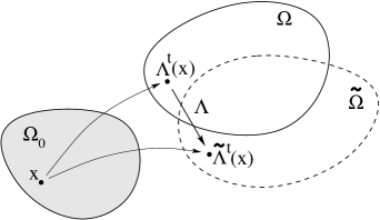
Figure 3: The diffeomorphisms $\Lambda^{t}$ and $\tilde{\Lambda}^{t}$ define the change of variable $\Lambda=\tilde{\Lambda}^{t}\circ(\Lambda^{t})^{-1}$

Combining the above inequality with (7.1) we finally obtain

$${\mbox{d}\over\mbox{d}t}\|\tilde{\Lambda}^{t}-\Lambda^{t}\|_{{\cal C}^{2,\alpha}(\Omega_{0})}~{}\leq~{}C\|\tilde{\Lambda}^{t}-\Lambda^{t}\|_{{\cal C}^{2,\alpha}(\Omega_{0})}.$$

By Gronwall’s inequality, this implies that $\tilde{\Lambda}^{t}=\Lambda^{t}$ for all times $t$ small enough. In turn, this implies the equalities $\tilde{w}(t,\cdot)=w(t,\cdot)$ and $\tilde{u}(t,\cdot)=u(t,\cdot)$. Likewise, $\tilde{\bf v}(t,\cdot)={\bf v}(t,\cdot)$, because of the normalization (6.20). Applying the same argument on consecutive, sufficiently short time intervals, we conclude that $(\widetilde{\Omega},\tilde{\bf v},\tilde{w})=(\Omega,{\bf v},w)$ on the entire interval $t\in[0,T]$. MM     

8 Examples

We consider here two easy cases where the growth system can be solved explicitly. Example 1. Assume that the volumetric growth rate is proportional to the density of the morphogen, so that $g(u)=au$ in (E) with some $a>0$. Then the volume of $\Omega(t)$ grows at a constant rate. Indeed, (G) and (4.43) give

$$\begin{split}{\mbox{d}\over\mbox{d}t}\hbox{vol}\,\Omega(t)~{}&=~{}{\mbox{d}\over\mbox{d}t}\int_{\Omega_{0}}\det\nabla\Lambda^{t}(x)~{}\mbox{d}x~{}=~{}\int_{\Omega_{0}}\big{(}\det\nabla\Lambda^{t}(x)\big{)}\hbox{div}\,{\bf v}(t,\Lambda^{t}(x))~{}\mbox{d}x~{}\\ &=~{}\int_{\Omega(t)}\hbox{div}\,{\bf v}(t,x)~{}\mbox{d}x,\end{split}$$

while from (2.1) and since the conservation equation (H) enjoys the solution formula (4.41), it follows that

$$\int_{\Omega(t)}u(t,x)\,\mbox{d}x~{}=~{}\int_{\Omega(t)}(\Delta u+w)(t,x)\,\mbox{d}x~{}=~{}\int_{\Omega(t)}w(t,x)\,\mbox{d}x~{}=~{}\int_{\Omega_{0}}w_{0}(x)\,\mbox{d}x\,.$$

Concluding, the linear response function $g$ yields

$${\mbox{d}\over\mbox{d}t}\hbox{vol}\,\Omega(t)=a\int_{\Omega_{0}}w_{0}(x)\,\mbox{d}x=a\kappa_{0}\hbox{vol}\,\Omega_{0}\qquad\mbox{ where }\quad\kappa_{0}\doteq-\!\!\!\!\!\!\int_{\Omega_{0}}w_{0}(x)\,\mbox{d}x\,.$$ (8.1)

As a special case, assume that the initial domain $\Omega_{0}$ is a ball centered at the origin with radius $r_{0}>0$, and the initial density $w_{0}$ of signaling cells is radially symmetric. By uniqueness (up to a rigid motion), the density $w(t,\cdot)$ remains then radially symmetric for all $t>0$, whereas the domain $\Omega(t)$ remains a ball whose radius $r(t)$ may be determined from (8.1), namely: $r(t)^{d}=(1+\kappa_{0}at)r_{0}^{d}$.

In particular, when $w_{0}(x)\equiv w_{0}>0$ is constant, then the quantities

$$\begin{split}&\Lambda^{t}(x)=(1+w_{0}at)^{1/d}x,\qquad\Omega(t)=B\big{(}0,(1+w_{0}at)^{1/d}\big{)},\\ &u(t,x)=w(t,x)=\frac{w_{0}}{1+w_{0}at},\\ &{\bf v}(t,x)=\frac{w_{0}a}{d(1+w_{0}at)}x\quad\mbox{ and }\quad p(t,x)=\frac{w_{0}a}{d(1+w_{0}at)}\end{split}$$ (8.2)

provide the unique normalised solution to (M-E-H-G). Example 2. Next, assume that the growth rate $g:{\mathbb{R}}\to[0,\infty)$ is an arbitrary function satisfying (2.2), while the initial density $w_{0}$ of signaling cells is again constant on an arbitrary domain $\Omega_{0}$ with center of mass at $0$, so that: $\int_{\Omega_{0}}x~{}\mbox{d}x=0$. In this case, for every $t\geq 0$ the density $w(t,x)=w(t)$ is spatially constant over the domain $\Omega(t)$ and it satisfies the ODE

$$\dot{w}=-g(w)w\,,\qquad\qquad w(0)=w_{0}\,.$$ (8.3)

Indeed, generalizing (8.2) we have that

$$\begin{split}&\Lambda^{t}(x)=\Big{(}\frac{w_{0}}{w(t)}\Big{)}^{1/d}x,\qquad\Omega(t)=\Big{(}\frac{w_{0}}{w(t)}\Big{)}^{1/d}\Omega_{0},\\ &u(t,x)=w(t,x)=w(t),\\ &{\bf v}(t,x)=\frac{g(w(t))}{d}x\quad\mbox{ and }\quad p(t,x)=\frac{g(w(t))}{d}\end{split}$$

solve (M-E-H-G) together with (6.20). We further observe that setting:

$$w_{min}\doteq\max\{w\leq w_{0};~{}g(w)=0\}\geq 0,$$

the solution to (8.3) satisfies $w(t)\to w_{min}$ as $t\to\infty$. Consequently, if $w_{min}=0$ then $\Omega(t)$ becomes unbounded and its volume approaches infinity. On the other hand, if $w_{min}>0$ then $\Omega(t)$ increases to a finite limit $\Omega_{\infty}=\big{(}\frac{w_{0}}{w_{min}}\big{)}^{1/d}\Omega_{0}$.

9 The Lagrangian formulation

In this section, we reformulate the coupled variational-transport problem (M-E-H-G) using the Lagrangian variable $\xi\in\Omega_{0}$ labeling points in the initial domain.

Let $\Lambda:[0,T]\times\Omega_{0}\to{\mathbb{R}}^{d}$ be the solution to the problem in (G), as in (4.40):

$$\frac{\mbox{d}}{\mbox{d}t}\Lambda(t,\xi)={\bf v}(t,\Lambda(t,\xi)),\qquad\Lambda(0,\xi)=\xi.$$ (9.1)

Define, for small $t\in[0,T]$, a flow of Riemann metrics $g:[0,T]\times\Omega_{0}\to{{\mathbb{R}}}^{d\times d}_{sym,>}$, by setting

$$g(t,\xi)=\big{(}(\nabla\Lambda)^{T}\nabla\Lambda\big{)}(t,\xi).$$ (9.2)

The Christoffel symbols of $g$ are given through: $\partial_{ij}\Lambda=\sum_{m=1}^{d}\Gamma_{ij}^{m}\partial_{m}\Lambda$ or, in vector notation:

$$\Gamma_{ij}^{\cdot}=(\nabla\Lambda)^{-1}\partial_{ij}\Lambda\qquad\hbox{for all}~{}i,j:1\ldots d.$$

We pull-back the solution quantities of the system (M-E-H-G) on $\Omega_{0}$:

$$\tilde{w}(t,\xi)=w(t,\Lambda(t,\xi)),\quad\tilde{u}(t,\xi)=u(t,\Lambda(t,\xi)),\quad\tilde{{\bf v}}(t,\xi)=\nabla\Lambda(t,\xi)^{-1}{\bf v}(t,\Lambda(t,\xi))$$ (9.3)

and seek for their equivalent description (M1-E1-H1-G1) below. There are some advantages in doing this:

• A solution is a time-dependent field of $d\times d$ matrices $g=[g_{ij}]$ on the fixed domain $\Omega_{0}$.

• The transport equation (H) has a trivial solution.

• The non-uniqueness is automatically removed, since adding a rigid motion to the map $\xi\mapsto\Lambda(t,\xi)$ does not affect $g_{ij}$.

• In Eulerian coordinates, the solution may cease to exist in finite time because different portions of the growing set may overlap. This issue does not arise when working in Lagrangian coordinates.

On the other hand, while in Eulerian coordinates the elliptic equation (2.1) and the system (4.8) have constant coefficients, in Lagrangian coordinates these coefficients depend on the metric itself. This makes the analysis considerably more difficult.

1. By Lemma 4.5 and since $\det g=(\det\nabla\Lambda)^{2}$, we get:

$$\tilde{w}(t,\xi)=\frac{w_{0}(\xi)}{\sqrt{\det g(t,\xi)}}.$$ (H1)

To deal with (M), we observe equality of (the row) vectors in: $\nabla u=(\nabla\tilde{u})(\nabla\Lambda)^{-1}$, so that:

$$|\nabla u(t,\Lambda(t,\xi))|^{2}=\big{\langle}(\nabla\tilde{u})(\nabla\Lambda)^{-1}(\nabla\Lambda)^{-1,T},\nabla\tilde{u}\big{\rangle}=\big{\langle}(\nabla\tilde{u})g^{-1},\nabla\tilde{u}\big{\rangle}(t,\xi).$$

Changing the variables in (M) results in:

$$\begin{split}J(u(t,\cdot))&=\int_{\Omega_{0}}\Big{(}\frac{|\nabla u|^{2}}{2}+\frac{u^{2}}{2}-wu\Big{)}(t,\Lambda(t,\xi))\det\nabla\Lambda(t,\xi)~{}\mbox{d}\xi\\ &=\int_{\Omega_{0}}\Big{(}\frac{1}{2}\big{\langle}(\nabla\tilde{u})g^{-1},\nabla\tilde{u}\big{\rangle}+\frac{1}{2}|\tilde{u}(t,\xi)|^{2}-\tilde{w}\tilde{u}\Big{)}\sqrt{\det g(t,\xi)}~{}\mbox{d}\xi,\end{split}$$

so that the minimization problem becomes:

$$\mbox{minimize:}\qquad\tilde{J}(t,\tilde{u})=\int_{\Omega_{0}}\Big{(}\frac{\big{\langle}(\nabla\tilde{u})g^{-1},\nabla\tilde{u}\Big{\rangle}}{2}+\frac{|\tilde{u}|^{2}}{2}-\tilde{w}\tilde{u}\big{)}\sqrt{\det g(t,\xi)}~{}\mbox{d}\xi.$$ (M1)

2. To rewrite (E), differentiate the (column vector) equality ${\bf v}(t,\Lambda(t,\xi))=(\nabla\Lambda)\tilde{{\bf v}}(t,\xi)$ in $\xi$:

$$\begin{split}&\nabla{\bf v}(t,\Lambda(t,\xi))\\ &=(\nabla\Lambda)(\nabla\tilde{{\bf v}})(\nabla\Lambda)^{-1}(t,\xi)+\Big{[}(\partial_{2}\nabla\Lambda)\tilde{{\bf v}},(\partial_{1}\nabla\Lambda)\tilde{{\bf v}},\ldots,(\partial_{d}\nabla\Lambda)\tilde{{\bf v}}\Big{]}(\nabla\Lambda)^{-1}(t,\xi)\\ &=(\nabla\Lambda)\Bigg{[}\nabla\tilde{{\bf v}}+\Big{[}(\nabla\Lambda)^{-1}(\partial_{2}\nabla\Lambda)\tilde{{\bf v}},(\nabla\Lambda)^{-1}(\partial_{1}\nabla\Lambda)\tilde{{\bf v}},\ldots,(\nabla\Lambda)^{-1}(\partial_{d}\nabla\Lambda)\tilde{{\bf v}}\Big{]}\Bigg{]}(\nabla\Lambda)^{-1}(t,\xi)\\ &=(\nabla\Lambda)(\tilde{\nabla}\tilde{{\bf v}})(\nabla\Lambda)^{-1}(t,\xi),\end{split}$$ (9.4)

where $\tilde{\nabla}\tilde{{\bf v}}=\{\tilde{v}^{i}_{,j}\}_{i,j=1\ldots d}$ is the covariant derivative of the vector field $\tilde{{\bf v}}=\{\tilde{v}^{i}\}_{i=1\ldots d}$ with respect to the metric $g$, in matrix notation given by:

$$\tilde{\nabla}\tilde{{\bf v}}=\nabla\tilde{{\bf v}}+\Bigg{[}\Big{[}\Gamma_{11}^{\cdot},\Gamma_{12}^{\cdot},\ldots,\Gamma_{1d}^{\cdot}\Big{]}\tilde{{\bf v}},\ldots,\Big{[}\Gamma_{j1}^{\cdot},\Gamma_{j2}^{\cdot},\ldots,\Gamma_{jd}^{\cdot}\Big{]}\tilde{{\bf v}},\ldots,\Big{[}\Gamma_{d1}^{\cdot},\Gamma_{d2}^{\cdot},\ldots,\Gamma_{dd}^{\cdot}\Big{]}\tilde{{\bf v}}\Bigg{]},$$

so that $[\tilde{\nabla}\tilde{{\bf v}}]_{ij}=\tilde{v}^{i}_{,j}=\partial_{j}\tilde{v}^{i}+\sum_{m=1}^{d}\Gamma_{jm}^{i}\tilde{v}^{m}$. We thus obtain:

$$\begin{split}|\mbox{sym}\nabla{\bf v}|&{}^{2}(t,\Lambda(t,\xi))=~{}\frac{1}{4}\Big{(}\big{\langle}(\nabla\Lambda)(\tilde{\nabla}\tilde{{\bf v}})(\nabla\Lambda)^{-1}:(\nabla\Lambda)(\tilde{\nabla}\tilde{{\bf v}})(\nabla\Lambda)^{-1}\big{\rangle}\\ &\qquad\qquad\qquad\qquad+2\big{\langle}(\nabla\Lambda)(\tilde{\nabla}\tilde{{\bf v}})(\nabla\Lambda)^{-1}:(\nabla\Lambda)^{-1,T}(\tilde{\nabla}\tilde{{\bf v}})^{T}(\nabla\Lambda)^{T}\big{\rangle}\\ &\qquad\qquad\qquad\qquad+\big{\langle}(\nabla\Lambda)^{-1,T}(\tilde{\nabla}\tilde{{\bf v}})(\nabla\Lambda)^{T}:(\nabla\Lambda)^{-1,T}(\tilde{\nabla}\tilde{{\bf v}})^{T}(\nabla\Lambda)^{T}\big{\rangle}\Big{)}\\ &=\frac{1}{2}\Big{(}\big{\langle}g(\tilde{\nabla}\tilde{{\bf v}})g^{-1}:\tilde{\nabla}\tilde{{\bf v}}\big{\rangle}+\big{\langle}\tilde{\nabla}\tilde{{\bf v}}:(\tilde{\nabla}\tilde{{\bf v}})^{T}\big{\rangle}\Big{)}=\frac{1}{2}\Big{(}\big{\langle}g(\tilde{\nabla}\tilde{{\bf v}})g^{-1}:\tilde{\nabla}\tilde{{\bf v}}\big{\rangle}+\mbox{trace}\big{(}(\tilde{\nabla}\tilde{{\bf v}})^{2}\big{)}\Big{)}.\end{split}$$

Consequently, changing the variables in (E) yields:

$$\begin{split}E({\bf v}(t,\cdot))&=\frac{1}{2}\int_{\Omega_{0}}\big{|}\mbox{sym}\nabla{\bf v}(t,\Lambda(t,\xi))|^{2}\det\nabla\Lambda(t,\xi)~{}\mbox{d}\xi\\ &=\frac{1}{4}\int_{\Omega_{0}}\Big{(}\big{\langle}g(\tilde{\nabla}\tilde{{\bf v}})g^{-1}:\tilde{\nabla}\tilde{{\bf v}}\big{\rangle}+\mbox{trace}\big{(}(\tilde{\nabla}\tilde{{\bf v}})^{2}\big{)}\Big{)}(t,\xi)\sqrt{\det g(t,\xi)}~{}\mbox{d}\xi.\end{split}$$

We further get:

$$\mbox{div }{\bf v}(t,\Lambda(t,\xi))=\mbox{trace}\nabla{\bf v}(t,\Lambda(t,\xi))=\mbox{trace}\tilde{\nabla}\tilde{{\bf v}}(t,\xi)=\widetilde{\mbox{div }}\tilde{{\bf v}}(t,\xi),$$

where the covariant divergence of the vector field $\tilde{v}$ is given by:

$$\widetilde{\mbox{div }}\tilde{{\bf v}}=\mbox{div}\nabla\tilde{{\bf v}}+\sum_{k,i=1\ldots d}\Gamma_{ki}^{k}\tilde{v}^{i}=\hbox{div}\,\nabla\tilde{\bf v}+\langle\nabla\big{(}\ln\sqrt{\det g}\big{)},\tilde{\bf v}\rangle.$$

The minimization problem (E) hence becomes:

$$\begin{split}\mbox{minimize:}\qquad&\tilde{E}(t,\tilde{{\bf v}})=\frac{1}{4}\int_{\Omega_{0}}\Big{(}\big{\langle}g(\tilde{\nabla}\tilde{{\bf v}})g^{-1}:\tilde{\nabla}\tilde{{\bf v}}\big{\rangle}+\mbox{trace}\big{(}(\tilde{\nabla}\tilde{{\bf v}})^{2}\big{)}\Big{)}\sqrt{\det g(t,\xi)}~{}\mbox{d}\xi\\ &\mbox{ with }\quad\widetilde{\mbox{div }}\tilde{{\bf v}}=\tilde{u}.\end{split}$$ (E1)

We observe in passing that the integrand in (E1) above depends only on the symmetric part of the covariant derivative $\tilde{\nabla}\tilde{{\bf v}}_{*}$ of the covariant tensor $\tilde{{\bf v}}_{*}=g\tilde{{\bf v}}$, carrying the resemblance to the original functional in (E). Indeed, since $\tilde{\nabla}\tilde{{\bf v}}_{*}=\tilde{\nabla}(g\tilde{{\bf v}})=g\tilde{\nabla}\tilde{{\bf v}}$, then $\tilde{\nabla}\tilde{{\bf v}}=g^{-1}\tilde{\nabla}\tilde{{\bf v}}_{*}$, and:

$$\begin{split}\big{\langle}g(\tilde{\nabla}\tilde{{\bf v}})&g^{-1}:\tilde{\nabla}\tilde{{\bf v}}\big{\rangle}+\mbox{trace}\big{(}(\tilde{\nabla}\tilde{{\bf v}})^{2}\big{)}=\big{\langle}g^{-1}(\tilde{\nabla}\tilde{{\bf v}}_{*})g^{-1}:\tilde{\nabla}\tilde{{\bf v}}_{*}\big{\rangle}+\mbox{trace}\big{(}(g^{-1}\tilde{\nabla}\tilde{{\bf v}}_{*})^{2}\big{)}\\ &=\big{\langle}g^{-1}(\tilde{\nabla}\tilde{{\bf v}}_{*})g^{-1}:\tilde{\nabla}\tilde{{\bf v}}\big{\rangle}+\big{\langle}g^{-1}(\tilde{\nabla}\tilde{{\bf v}}_{*})g^{-1}:(\tilde{\nabla}\tilde{{\bf v}}_{*})^{T}\big{\rangle}\\ &=2\big{\langle}g^{-1}(\tilde{\nabla}\tilde{{\bf v}}_{*})g^{-1}:\mbox{sym}\tilde{\nabla}\tilde{{\bf v}}\big{\rangle}=2\big{\langle}g^{-1}(\mbox{sym}\tilde{\nabla}\tilde{{\bf v}}_{*})g^{-1}:\mbox{sym}\tilde{\nabla}\tilde{{\bf v}}\big{\rangle}.\end{split}$$

3. The rule (G) is being replaced by the equation for the evolution of the metric:

$$\begin{split}\frac{\mbox{d}}{\mbox{d}t}g(t,\xi)&=\frac{\mbox{d}}{\mbox{d}t}\big{(}(\nabla\Lambda)^{T}\nabla\Lambda\big{)}(t,\Lambda(t,\xi))\\ &=\big{(}\nabla{\bf v}(t,\Lambda(t,\xi))\nabla\Lambda(t,\xi)\big{)}^{T}\nabla\Lambda+(\nabla\Lambda)^{T}\nabla{\bf v}(t,\Lambda(t,\xi))\nabla\Lambda(t,\xi)\\ &=(\tilde{\nabla}\tilde{{\bf v}})^{T}g+g(\tilde{\nabla}\tilde{{\bf v}})=2~{}\mbox{sym}\big{(}g(\tilde{\nabla}\tilde{{\bf v}})\big{)}(t,\xi).\end{split}$$ (9.5)

We now conclude, by a direct calculation:

$$\begin{split}\frac{\mbox{d}}{\mbox{d}t}g(t,\xi)=2~{}\mbox{sym}\big{(}g\nabla\tilde{{\bf v}}\big{)}+\sum_{i=1}^{d}(\partial_{i}g)\tilde{v}^{i}.\end{split}$$ (G1)

10 Modeling the growth of a 2-dimensional surface in ${\mathbb{R}}^{3}$

We now generalize the model (M-E-H-G) to the case where, instead of an open domain $\Omega(t)\subset{\mathbb{R}}^{d}$, the growing set is a codimension-one manifold $S(t)$. For simplicity, we assume that $d=3$, so that $S(t)$ is a two-dimensional surface in ${\mathbb{R}}^{3}$. 1. Again, for each $t\in[0,T]$ we denote by $w(t,\cdot):S(t)\to{\mathbb{R}}$ a nonnegative function representing the density of the signaling cells in the tissue, whereas $u(t,\cdot):S(t)\to{\mathbb{R}}$ is the concentration of produced morphogen. This function $u(t,\cdot)$ is defined to be the minimizer of

$$\hbox{minimize:}\quad J(u)=\int_{S(t)}\Big{(}{|\nabla u|^{2}\over 2}+{u^{2}\over 2}-wu\Big{)}~{}\mbox{d}\sigma(x),$$ (M2)

or, equivalently, the solution to:

$$\left\{\begin{array}[]{ll}\Delta_{LB}u-u+w=0&x\in S(t)\cr\langle\nabla u,\nu\rangle=0&x\in\partial S(t).\end{array}\right.$$ (10.1)

Here $\nu\in T_{x}S$ is the normal vector to the boundary $\partial S$, and $\Delta_{LB}u$ stands for the Laplace-Beltrami operator acting on the scalar field $u$ on $S$.

Consider a chart of $S$, so that $S=y(\omega)$ is parametrized by an immersion $y:\omega\to{\mathbb{R}}^{3}$ for some open set $\omega\subset{\mathbb{R}}^{2}$. We recall that the Laplace-Beltrami operator is given by

$$\Delta_{LB}u=\left[\displaystyle{\frac{1}{\sqrt{\det g}}}\sum_{i,j=1}^{2}\partial_{i}\Big{(}\sqrt{\det g}~{}g^{ij}\partial_{j}(u\circ y)\Big{)}\right]\circ y^{-1}.$$

On the domain $\omega$ of the chart, we denote by $[g_{ij}]_{i,j=1,2}=(\nabla y)^{T}\nabla y$ the pull-back metric $g$ of the Euclidean metric $I$ restricted to $S$, while its inverse is denoted by $[g^{ij}]_{i,j=1,2}=\bigl{(}(\nabla y)^{T}\nabla y\bigr{)}^{-1}$.

2. To determine the velocity ${\bf v}(t,\cdot):S(t)\to{\mathbb{R}}^{3}$, we first derive the compressibility constraint expressing the fact that the infinitesimal change of the surface area element due to the family of deformations $\Lambda_{\epsilon}=id+\epsilon{\bf v}:S\to{\mathbb{R}}^{3}$ as $\epsilon\to 0$, equals $u$.

Fix $t\in[0,T]$ and consider a flow of deformed surfaces $\epsilon\mapsto\Lambda_{\epsilon}(S)$, starting from $S=S(t)$. For a given point $x\in S$, let $\{\tau_{1}(x),\tau_{2}(x)\}$ be an orthonormal basis of the tangent space $T_{x}S$. Calling ${\bf n}$ the unit normal vector to $S$, we compute

$$\begin{split}|\partial_{\tau_{1}}\Lambda_{\epsilon}\times\partial_{\tau_{2}}\Lambda_{\epsilon}|~{}&=~{}|(\tau_{1}+\epsilon\partial_{\tau_{1}}{\bf v})\times(\tau_{2}+\epsilon\partial_{\tau_{2}}{\bf v})|\\ &=~{}|(\tau_{1}\times\tau_{2})+\epsilon(\partial_{\tau_{1}}{\bf v}\times\tau_{2}-\partial_{\tau_{2}}{\bf v}\times\tau_{1})+\mathcal{O}(\epsilon^{2})|\\ &=~{}\Big{(}|\tau_{1}\times\tau_{2}|^{2}+2\epsilon\big{\langle}\tau_{1}\times\tau_{2},\partial_{\tau_{1}}{\bf v}\times\tau_{2}-\partial_{\tau_{2}}{\bf v}\times\tau_{1}\big{\rangle}+\mathcal{O}(\epsilon^{2})\Big{)}^{1/2}\\ &=~{}|\tau_{1}\times\tau_{2}|\Big{(}1+2\epsilon\big{\langle}\frac{\tau_{1}\times\tau_{2}}{|\tau_{1}\times\tau_{2}|^{2}},\partial_{\tau_{1}}{\bf v}\times\tau_{2}-\partial_{\tau_{2}}{\bf v}\times\tau_{1}\big{\rangle}+\mathcal{O}(\epsilon^{2})\Big{)}^{1/2}\\ &=~{}|\tau_{1}\times\tau_{2}|\Big{(}1+\epsilon\big{\langle}\frac{\tau_{1}\times\tau_{2}}{|\tau_{1}\times\tau_{2}|^{2}},\partial_{\tau_{1}}{\bf v}\times\tau_{2}-\partial_{\tau_{2}}{\bf v}\times\tau_{1}\big{\rangle}+\mathcal{O}(\epsilon^{2})\Big{)}\\ &=~{}|\tau_{1}\times\tau_{2}|+\epsilon\big{\langle}{\bf n},\partial_{\tau_{1}}{\bf v}\times\tau_{2}-\partial_{\tau_{2}}{\bf v}\times\tau_{1}\big{\rangle}+\mathcal{O}(\epsilon^{2}).\end{split}$$

By suitably choosing the orientation of ${\bf n}$, we can assume that $\{\tau_{1},\tau_{2},{\bf n}\}$ is a positively oriented orthonormal basis of ${\mathbb{R}}^{3}$. Therefore

$$\begin{split}\lim_{\epsilon\to 0}\frac{|\partial_{\tau_{1}}\Lambda_{\epsilon}\times\partial_{\tau_{2}}\Lambda_{\epsilon}|-|\tau_{1}\times\tau_{2}|}{\epsilon}~{}&=~{}\big{\langle}{\bf n},\partial_{\tau_{1}}{\bf v}\times\tau_{2}-\partial_{\tau_{2}}{\bf v}\times\tau_{1}\big{\rangle}\\ &=~{}\big{\langle}\partial_{\tau_{1}}{\bf v},\tau_{2}\times{\bf n}\big{\rangle}-\big{\langle}\partial_{\tau_{2}}{\bf v},\tau_{1}\times{\bf n}\big{\rangle}\\ &=~{}\big{\langle}\partial_{\tau_{1}}{\bf v},\tau_{1}\big{\rangle}+\big{\langle}\partial_{\tau_{2}}{\bf v},\tau_{2}\big{\rangle}.\end{split}$$

We now decompose the vector field ${\bf v}={\bf v}_{tan}+v_{3}{\bf n}$ into a tangential component ${\bf v}_{tan}(x)\in T_{x}S$ and a normal component, given by a scalar field $v_{3}:S\to{\mathbb{R}}$. Then

$$\begin{split}\big{\langle}\partial_{\tau_{1}}{\bf v},\tau_{1}\big{\rangle}+\big{\langle}\partial_{\tau_{2}}{\bf v},\tau_{2}\big{\rangle}&~{}=~{}\big{\langle}\partial_{\tau_{1}}{\bf v}_{tan},\tau_{1}\big{\rangle}+\big{\langle}\partial_{\tau_{2}}{\bf v}_{tan},\tau_{2}\big{\rangle}+v_{3}\Big{(}\langle\partial_{\tau_{1}}{\bf n},\tau_{1}\rangle+\langle\partial_{\tau_{2}}{\bf n},\tau_{2}\rangle\Big{)}\\ &~{}=~{}\big{\langle}\partial_{\tau_{1}}{\bf v}_{tan},\tau_{1}\big{\rangle}+\big{\langle}\partial_{\tau_{2}}{\bf v}_{tan},\tau_{2}\big{\rangle}+v_{3}\Big{(}\langle\Pi{\tau_{1}},\tau_{1}\rangle+\langle\Pi{\tau_{2}},\tau_{2}\rangle\Big{)}\\ &~{}=~{}\hbox{div}\,{\bf v}_{tan}+v_{3}\mbox{trace~{}}\Pi~{}=~{}\hbox{div}\,{\bf v}_{tan}+2Hv_{3},\end{split}$$

where $\Pi=\nabla{\bf n}$ is the shape operator on $S$ and $H=\frac{1}{2}\mbox{trace }\Pi$ is the mean curvature of $S$. The constraint on ${\bf v}$ accounting for area growth can thus be written in the form

$$\hbox{div}\,{\bf v}_{tan}+2Hv_{3}~{}=~{}u.$$ (10.2)

To find an appropriate replacement of (E) in the present setting, consider the following model of elastic energy of deformations $\Lambda:S\to{\mathbb{R}}^{3}$ of $S$, given by

$$I(\Lambda)~{}=~{}\int_{S}\mbox{dist}^{2}\big{(}\nabla\Lambda(x),O(2,3)\big{)}~{}\mbox{d}\sigma(x).$$

Here $O(2,3)=\{F\in{\mathbb{R}}^{3\times 2};~{}F^{T}F=I\}$ represents gradients of deformations that preserve the metric on $S$. The integrand $\mbox{dist}^{2}(\cdot\,,O(2,3))$ may be replaced by some other quadratic function reflecting the material properties of the shell, provided it still satisfies the frame invariance and some other minimal regularity conditions.

Consider the expansion $\Lambda=id+\epsilon{\bf v}$. Then, in analogy to the result in [12], we claim that the scaled functionals $\epsilon^{-2}I$ $\Gamma$-converge as $\epsilon\to 0$ to the following elastic energy on $S$:

$$E({\bf v})~{}=~{}\frac{1}{2}\int_{S}|\hbox{sym}\,\nabla{\bf v}_{tan}+v_{3}\Pi|^{2}~{}\mbox{d}\sigma(x).$$ (10.3)

Among all velocity fields ${\bf v}$ which satisfy (10.2), by the previous analysis we should thus choose one which minimizes (10.2). In the present setting, the constrained minimization (E) should be replaced by

$$\hbox{minimize:}\quad\int_{S}|\hbox{sym}\,\nabla{\bf v}_{tan}+v_{3}\Pi|^{2}~{}\mbox{d}\sigma(x),\quad\qquad\hbox{subject to:}\quad\hbox{div}\,{\bf v}_{tan}+2Hv_{3}=u.$$ (E2)

3. The evolving surface $S(t)$ is now recovered as the set reached by trajectories of ${\bf v}$ starting in $S(0)$. Namely,

$$S(t)~{}=~{}\bigg{\{}\Lambda^{t}(x)\,;\quad\Lambda^{t}(0)=x\in S(0)~{}\mbox{ and }~{}\frac{\mbox{d}}{\mbox{d}s}\Lambda^{s}(x)={\bf v}(s,\Lambda^{s}(x))~{}~{}\hbox{for all}~{}s\in[0,t]\bigg{\}}.$$ (G2)

Again, the morphogen-producing cells are transported along the flow, so that their density satisfies

$$w(t,\Lambda^{t}(x))=\frac{w(0,x)}{\det\nabla\Lambda^{t}(x)}\qquad\mbox{for all }~{}x\in S(0),~{}t\in[0,T],$$ (H2)

where $\det\nabla\Lambda^{t}(x)$ is the Jacobian of the linear map $\nabla\Lambda^{t}(x):T_{x}S(0)\to T_{\Lambda^{t}(x)}S(t)$.

In conclusion, we propose (M2-E2-G2-H2) as a model for thin shell/surface growth. We leave the resulting system of PDEs as a topic for future study.

Remark 10.1.

(i) In the flat case $S\subset{\mathbb{R}}^{2}$ and assuming the in-plane evolution to the effect that $v_{3}=0$, the constraint (10.2) becomes: $\hbox{div}\,{\bf v}=u$, which is precisely the constraint in (E). In the general case, the infinitesimal change of area decouples into the in-surface part $\mbox{div }{\bf v}_{tan}$, and $2Hv_{3}$. Note that if $S$ is a minimal surface then all its variations (preserving the boundary) yield zero infinitesimal change of total area, so in view of (10.2) we get $\int_{S}Hv_{3}=0$ for every $v_{3}$ vanishing on $\partial S$. Thus $H\equiv 0$, as expected.

(ii) The problem (10.2) is under-determined (one equation in three unknowns). Representing ${\bf v}_{tan}=\nabla\psi$ as the gradient of a scalar field $\psi$ on $S$, the equation (10.2) can be replaced by the Laplace-Beltrami equation

$$\Delta_{LB}\psi~{}=~{}u-2Hv_{3}\,.$$

(iii) The energy functional $E({\bf v})$ in (10.3) measures stretching, i.e. the change in metric on $S$ after the deformation to $\Lambda_{\epsilon}(S)$, of order $\epsilon$. This functional can be augmented by adding the bending term at a higher order:

$$\bar{E}({\bf v})=\frac{1}{2}\int_{S}|\hbox{sym}\,\nabla{\bf v}_{tan}+v_{3}\Pi|^{2}~{}\mbox{d}\sigma(x)+\frac{\mu}{24}\int_{S}|\big{(}\nabla((\nabla{\bf v}){\bf n})-(\nabla{\bf v})\Pi\big{)}_{tan}|^{2}~{}\mbox{d}\sigma(x).$$ (10.4)

The integrand in the second term above measures the difference of order $\epsilon$ between the shape operator $\Pi$ on $S$ and the shape operator $\Pi_{\epsilon}$ of $\Lambda_{\epsilon}(S)=id+\epsilon{\bf v}$. Alternatively, the tensor under this integral represents the linear map: $T_{x}S\ni\tau\mapsto\big{(}\partial_{\tau}(\nabla{\bf v})\big{)}{\bf n}\in T_{x}S$. The presence of a bending term introduces a regularizing effect, while the prefactor $\frac{\mu}{24}$, which is a fixed small “viscosity” parameter, guarantees that bending contributes at a higher order than stretching.

Let us also mention that a potentially relevant to the problem at hand discussion of the $2$-dimensional models of elastic shells and their relation to the $3$d nonlinear elasticity, also in presence of prestrain which is effectively manifested through the constraints of the type (10.2), can be found in the review paper [18] and references therein.

Acknowledgments. The first author was partially supported by NSF grant DMS-1714237, “Models of controlled biological growth”. The second author was partially supported by NSF grants DMS-1406730 and DMS-1613153.

References

- [1] S. Agmon, A. Douglis, and L. Nirenberg, Estimates near the boundary for solutions of elliptic partial differential equations satisfying general boundary conditions II, Comm. Pure Appl. Math. 17, (1964), 35–92.
- [2] D. Ambrosi, G. Ateshian, E. Arruda, S. Cowin, J. Dumais, A. Goriely, G. Holzapfel, J. Humphrey, R. Kemkemer, E. Kuhl, J. Olberding, L. Taber, K. Garikipati, Perspectives on biological growth and remodeling. J. Mech. Phys. Solids 59 (2011), 863–883.
- [3] R. Baker and P. Maini, A mechanism for morphogen-controlled domain growth. J. Math. Biol. (2007), 597–622.
- [4] R. Baker, E. Gaffney, and P. Maini, Partial differential equations for self-organization in cellular and developmental biology. Nonlinearity 21 (2008), R251–R290.
- [5] G. Barles, P. Cardaliaguet, O. Ley, and A. Monteillet, Uniqueness results for nonlocal Hamilton-Jacobi equations. J. Funct. Anal. 257 (2009), 1261–1287.
- [6] B. Bazaliy, and A. Friedman, A free boundary problem for an elliptic-parabolic system: application to a model of tumor growth. Comm. Partial Differential Equations 28 (2003), 517–560.
- [7] M. Bergner, J. Escher, and F.M. Lippoth, On the blow up scenario for a class of parabolic moving boundary problems. Nonlinear Analysis 75 (2012), 3951–3963.
- [8] P. Cardaliaguet and O. Ley, Some flows in shape optimization. Arch. Rational Mech. Anal. 183 (2007), 21–58.
- [9] X. Chen and A. Friedman, A free boundary problem for an elliptic-hyperbolic system: an application to tumor growth. SIAM J. Math. Anal. 35 (2003), 974–986.
- [10] S. Cui and J. Escher, Well-posedness and stability of a multi-dimensional tumor growth model. Arch. Rational Mech. Anal. 191 (2009), 173–193.
- [11] S. Cui and A. Friedman, A free boundary problem for a singular system of differential equations: an application to a model of tumor growth. Trans. Am. Math. Soc. 355 (2002), 3537–3590.
- [12] G. Dal Maso, M. Negri and D. Percivale, Linearized elasticity as -Limit of finite elasticity, Set-Valued Analysis 10 (2002), 165–183.
- [13] J. Escher, Classical solutions for an elliptic parabolic system. Interfaces Free Bound. 6 (2004), 175–193.
- [14] A. Friedman, A free boundary problem for a coupled system of elliptic, hyperbolic, and Stokes equations modeling tumor growth. Interfaces and Free Boundaries 8 (2006), 247–261.
- [15] A. Friedman and F. Reitich, Analysis of a mathematical model for the growth of tumors. J. Math. Biol. 38 (1999), 262–284.
- [16] D. Gilbarg and N. S. Trudinger, Elliptic Partial Differential Equations of Second Order. Springer, Berlin, 2001.
- [17] O. A. Ladyzhenskaya, Linear and Quasilinear Elliptic Equations, Academic Press, 1968.
- [18] M. Lewicka and R. Pakzad, Prestrained elasticity: from shape formation to Monge-Ampere anomalies, Notices of the AMS, January 2016.
- [19] A. Lunardi, An introduction to parabolic moving boundary problems. Functional analytic methods for evolution equations, Springer Lecture Notes in Math. 1855 (2004), 371–399.
- [20] J. Prüss and G. Simonett, Moving Interfaces and Quasilinear Parabolic Evolution Equations, Birkhäuser, 2016.
- [21] R. Temam, Navier-Stokes Equations: Theory and Numerical Analysis, AMS Chelsea Publishing, 2010.