A-posteriori snapshot location for POD
in optimal control of linear parabolic equations

Abstract.

In this paper we study the approximation of an optimal control problem for linear parabolic PDEs with model order reduction based on Proper Orthogonal Decomposition (POD-MOR). POD-MOR is a Galerkin approach where the basis functions are obtained upon information contained in time snapshots of the parabolic PDE related to given input data. In the present work we show that for POD-MOR in optimal control of parabolic equations it is important to have knowledge about the controlled system at the right time instances. We propose to determine the time instances (snapshot locations) by an a-posteriori error control concept. This method is based on a reformulation of the optimality system of the underlying optimal control problem as a second order in time and fourth order in space elliptic system which is approximated by a space-time finite element method. Finally, we present numerical tests to illustrate our approach and to show the effectiveness of the method in comparison to existing approaches.

1. Introduction

Optimization with PDE constraints is nowadays a well-studied topic motivated by its relevance in industrial applications. We are interested in the numerical approximation of such optimization problems in an efficient and reliable way using surrogate models obtained with POD-MOR. The surrogate models are built upon snapshots of the system to provide information about the underlying problem. This stage is usually called the offline stage. For the snapshot POD approach we refer the reader to [28].
Several works focus their attention on the choice of the snapshots, in order to approximate either dynamical systems or optimal control problems by suitable surrogate models. In [19], it is proposed to optimize the choice of the time instances such that the error between POD and the trajectory of the dynamical system is minimized. A recent approach proposes to choose the snapshots by an a-posteriori error estimator in order to equidistribute the state error on the time grid related to the snapshot locations (see [13]). We also mention an adaptive method, proposed in [25], where the aim is to reduce expensive offline costs selecting the snapshots according to an adaptive time-stepping algorithm using time error-control. For further references we refer the interested reader to [25].
In optimal control problems the reduced model is usually built upon a forecast on the control. This approach does not guarantee a proper construction of the surrogate model since we do not know how far away the optimal solution is from the reference control. More sophisticated approaches select snapshots by solving an optimization problem in order to improve the selection of the snapshots according to the desired controlled dynamics. For this purpose optimality system for POD (OS-POD) is introduced in [18]. In OS-POD, the computation of the basis functions is performed by means of the solution of an enlarged optimal control problem which involves the full problem, the reduced equation and the eigenvalue problem for the POD modes.
The reduction of optimal control problems with particular focus on adaptive adjustments of the surrogate models can be found in [1, 4]. We should also mention another adaptive method for feedback control problems by means of the Hamilton-Jacobi-Bellman equation, introduced in [2].
Recently, an a-posteriori error estimator was introduced in [30, 14] for optimal control problems. In these works the error between the unknown optimal and the computed POD suboptimal control is estimated for linear and nonlinear problems, and it is shown that increasing the number of basis functions leads to the desired convergence. OS-POD and a-posteriori error estimation is combined in [32].
All these works have in common that they compute basis functions for optimal control problems. In our paper we address the question of an efficient and suitable selection of snapshot locations by means of an a-posteriori error control approach proposed in [7]. We rewrite the optimality conditions as a second order in time and fourth order in space elliptic equation for the adjoint variable and we generalize this approach to control constraints. In particular, a time adaptive concept is used to build the snapshot grid which should be used to construct the POD surrogate model for the approximate solution of the optimal control problem. Here the novelty for the reduced control problem is twofold: we directly obtain snapshots related to an approximation of the optimal control and, at the same time, we get information about the time grid.

We have proposed a similar approach based on a reformulation of the optimality system with respect to the state variable in [3]. Now, we focus our approach on the adjoint variable and generalize the idea presented in [7] to time dependent control intensities with control shape functions including control constraints. Furthermore, we certify our approach by means of several error bounds for the state, adjoint state and control variable.
The outline of this paper is as follows. In Section 2 we present the optimal control problem together with the optimality conditions. In Section 3 we recall the main results of [7]. Proper Orthogonal Decomposition and its application to optimal control problems is presented in Section 4. The focus of Section 5 lies in investigating our snapshot location strategy. Finally, numerical tests are discussed in Section 6 and conclusions are driven in Section 7.

2. Optimal Control Problem

In this section we describe the optimal control problem. The governing equation is given by a linear parabolic PDE:

$$\left.\begin{array}[]{rcll}y_{t}-\Delta y&=&f+\mathcal{B}u&\text{ in }\Omega_{T},\\ y(\cdot,0)&=&y_{0}&\text{ in }\Omega,\\ y&=&0&\text{ on }\Sigma_{T},\end{array}\right\}$$ (1)

where $\Omega\subset\mathbb{R}^{q},q\in\{1,2,3\}$ is an open bounded domain with smooth boundary, $T>0$, $\Omega_{T}:=\Omega\times(0,T]$ is the space-time cylinder, $\Sigma_{T}:=\partial\Omega\times(0,T]$, and the state is denoted by $y:\Omega_{T}\rightarrow\mathbb{R}$. As control space we use $\left(L^{2}(0,T;\mathbb{R}^{m}),\langle\cdot,\cdot\rangle_{U}\right)$, where $\langle u,v\rangle_{U}:=\sum_{i=1}^{m}\langle u_{i},v_{i}\rangle_{L^{2}(0,T)}$, and define the control operator as $\mathcal{B}:U\rightarrow L^{2}(0,T;H^{-1}(\Omega))$, $(\mathcal{B}u)(t)=\sum_{i=1}^{m}u_{i}(t)\chi_{i}$, where $\chi_{i}\in H^{-1}(\Omega)(1\leq i\leq m)$ denote specified control actions. Thus $\mathcal{B}$ is linear and bounded. For the control variable we require

$$u\in U_{ad}:=\{u\in U\;|\;u_{a}(t)\leq u(t)\leq u_{b}(t)\text{ in }\mathbb{R}^{m}\text{ a.e. in }[0,T]\}\subset L^{\infty}(0,T;\mathbb{R}^{m})$$

with $u_{a},u_{b}\in L^{\infty}(0,T;\mathbb{R}^{m}),u_{a}(t)\leq u_{b}(t)$ almost everywhere in $(0,T)$. It is well-known (see [20], for example) that for a given initial condition $y_{0}\in L^{2}(\Omega)$ and a forcing term $f\in L^{2}(0,T;H^{-1}(\Omega))$ the equation (1) admits a unique solution $y=y(u)\in W(0,T)$, where

$$W(0,T):=\left\{v\in L^{2}\left(0,T;H^{1}_{0}(\Omega)\right),\dfrac{\partial v}{\partial t}\in L^{2}\left(0,T;H^{-1}(\Omega)\right)\right\}.$$

If $y_{0}\in H_{0}^{1}(\Omega)$, higher regularity results can be derived according to [5]. We also note that the unconstrained case is related to $u_{a}\equiv-\infty,u_{b}\equiv+\infty$.

The weak formulation of (1) is given by: find $y\in W(0,T)$ with $y(0)=y_{0}$ and

$$\int_{\Omega}y_{t}(t)vdx+\int_{\Omega}\nabla y(t)\cdot\nabla vdx=\int_{\Omega}(f+\mathcal{B}u)(t)vdx\quad\forall v\in H_{0}^{1}(\Omega).$$ (2)

The cost functional we want to minimize is given by

$$J(y,u):=\dfrac{1}{2}\|y-y_{d}\|^{2}_{L^{2}(\Omega_{T})}+\dfrac{\alpha}{2}\|u\|^{2}_{U},$$ (3)

where $y_{d}\in L^{2}(\Omega_{T})$ is the desired state and the regularization parameter $\alpha$ is a real positive constant. The optimal control problem then reads

$$\min_{u\in U_{ad}}\hat{J}(u):=J(y(u),u)\mbox{, where }y(u)\mbox{ satisfies }\eqref{heat}.$$ (4)

Note that $U_{ad}$ is a non-empty, bounded, convex and closed subset of $L^{\infty}(0,T;\mathbb{R}^{m})$. Hence, it is easy to argue that (4) admits a unique solution $u\in U$ with associated state $y(u)\in W(0,T)$, see e.g. [20].

The first order optimality system of the optimal control problem (4) is given by the state equation (1), together with the adjoint equation

$$\left.\begin{array}[]{rcll}-p_{t}-\Delta p&=&y-y_{d}&\text{ in }\Omega_{T},\\ p(\cdot,T)&=&0&\text{ in }\Omega,\\ p&=&0&\text{ on }\Sigma_{T},\end{array}\right\}$$ (5)

and the variational inequality

$$\langle\alpha u+\mathcal{B}^{*}p,v-u\rangle_{U}\geq 0\quad\mbox{ for all }v\in U_{ad},$$ (6)

where $\mathcal{B}^{*}:L^{2}(0,T;H^{-1}(\Omega))^{*}\to U^{*}$ is the dual operator of $\mathcal{B}$. In (6) we have identified $L^{2}(0,T;H^{-1}(\Omega))^{*}$ with $L^{2}(0,T;H^{1}_{0}(\Omega))$ and $U^{*}$ with $U$, where we use that Hilbert spaces are reflexive. The variational inequality (6) is equivalent to the projection formula

$$u(t)=\mathcal{P}_{U_{ad}}\left\{-\dfrac{1}{\alpha}(\mathcal{B}^{*}p)(t)\right\}\mbox{ for almost all }t\in[0,T],$$ (7)

where $\mathcal{P}_{U_{ad}}:U\rightarrow U_{ad}$ denotes the orthogonal projection onto $U_{ad}$. It follows from the reflexivity of the involved spaces that the action of the adjoint operator $\mathcal{B}^{*}$ is given as

$$(\mathcal{B}^{*}v)(t)=\left(\langle\chi_{1},v\rangle_{H^{-1},H^{1}_{0}},\ldots,\langle\chi_{m},v\rangle_{H^{-1},H^{1}_{0}}\right)$$

and

$$\mathcal{P}_{U_{ad}}\left\{-\frac{1}{\alpha}\mathcal{B}^{*}p\right\}_{i}=\max\left\{u_{a},\min\{u_{b},-\frac{1}{\alpha}\langle\chi_{i},p\rangle_{H^{-1},H_{0}^{1}}\}\right\}.$$

Since our domain is smooth, the regularities of the optimal state, the optimal control and the associated adjoint state are limited through the regularities of the initial state $y_{0}$, the right hand side $f$, the control $\mathcal{B}u$ and the desired state $y_{d}.$
The numerical approximation of the optimality system (1)-(5)-(6) with a standard Finite Element Method (FEM) in the spatial variable leads to a high-dimensional system of ordinary differential equations:

$$\left.\begin{array}[]{rclrcl}M\dot{y}^{N}-Ay^{N}&=&f^{N}+\mathcal{B}^{N}u,&\quad y^{N}(0)&=&y_{0}^{N},\\ -M\dot{p}^{N}-Ap^{N}&=&y^{N}-y^{N}_{d},&\quad p^{N}(T)&=&0,\\ \langle\alpha u+(\mathcal{B}^{*})^{N}p^{N},v-u\rangle_{\mathcal{U}}&\geq&0.&&&\end{array}\right\}$$ (8)

Here $y^{N},p^{N}:[0,T]\rightarrow\mathbb{R}^{N}$ are the semi-discrete state and adjoint, respectively, $\dot{y}^{N},\dot{p}^{N}$ are the time derivatives, $M\in\mathbb{R}^{N\times N}$ denotes the mass matrix and $A\in\mathbb{R}^{N\times N}$ the stiffness matrix. Note that the dimension $N$ of each equation in the semi-discrete system (8) is related to the number of element nodes chosen in the FEM approach.

3. Space-Time approximation

In this section, we consider the reformulation of the optimality system (1)-(5)-(6) as an elliptic equation of fourth order in space and second order in time for the adjoint variable $p$. This is carried out for the unconstrained control problem in [7] and generalized to control constrained optimal control problems in [21]. Following these works, we include control constraints. Here, we aim to derive an a-posteriori error estimate for the time discretization as suggested in [7], which then turns out to be the basis for our model reduction approach to solve (4).
We define

$$H^{2,1}_{0}(\Omega_{T}):=\left\{v\in H^{2,1}(\Omega_{T}):v(T)=0\mbox{ in }\Omega\right\},$$

where

$$H^{2,1}(\Omega_{T})=L^{2}\left(0,T;H^{2}(\Omega\right)\cap H^{1}_{0}\left(\Omega)\right)\cap H^{1}\left(0,T;L^{2}(\Omega)\right)$$

is equipped with the norm

$$\|w\|_{H^{2,1}(\Omega_{T})}^{2}:=\left(\|w\|^{2}_{L^{2}(0,T;H^{2}(\Omega))}+\|w\|^{2}_{H^{1}(0,T;L^{2}(\Omega))}\right).$$

Under the assumptions $y_{0}\in H_{0}^{1}(\Omega)$, $\chi_{i}\in L^{2}(\Omega)$ for $i=1,\dotsc,m$ and $y_{d}\in H^{2,1}(\Omega_{T})$, the regularity of $y,p\in H^{2,1}(\Omega_{T})$ is ensured, see [5] for the details. Then, the first order optimality conditions (1)-(5)-(6) can be transformed into an initial boundary value problem for $p$ in space-time:

$$\left.\begin{array}[]{rcll}-p_{tt}+\Delta^{2}p-\mathcal{B}\mathcal{P}_{U_{ad}}\left(-\dfrac{1}{\alpha}\mathcal{B}^{*}p\right)&=&-(y_{d})_{t}+\Delta y_{d}&\text{ in }\Omega_{T},\\ p(\cdot,T)&=&0&\text{ in }\Omega,\\ p&=&0&\text{ on }\Sigma_{T},\\ \Delta p&=&y_{d}&\text{ on }\Sigma_{T},\\ \left(p_{t}+\Delta p\right)(0)&=&y_{d}(0)-y_{0}&\text{ in }\Omega,\end{array}\right\}$$ (9)

where, without loss of generality, we have set $f\equiv 0$. We note that the quantity

$$\mathcal{B}\mathcal{P}_{U_{ad}}\left(-\dfrac{1}{\alpha}\mathcal{B}^{*}p\right)$$

is nondifferentiable and nonlinear in $p$ and thus (9) becomes a semilinear second order in time and fourth order in space elliptic problem with a monotone nonlinearity. Existence of a unique weak solution for (9) can be proved analogously to [21] and follows from the fact that the optimal control problem (4) in the case of control constraints with closed and convex $U_{ad}\subset U$ admits a unique solution.
In order to provide the weak formulation of (9), we define the operator $A_{0}$ and the linear form $L_{0}$ as

$$A_{0}:H^{2,1}_{0}(\Omega_{T})\times H^{2,1}_{0}(\Omega_{T})\rightarrow\mathbb{R},\qquad L_{0}:H^{2,1}_{0}(\Omega_{T})\rightarrow\mathbb{R},$$

$$A_{0}(v,w):=\int_{\Omega_{T}}\left(v_{t}w_{t}-\mathcal{B}\mathcal{P}_{U_{ad}}\left(-\dfrac{1}{\alpha}\mathcal{B}^{*}v\right)w\right)+\int_{\Omega_{T}}\Delta v\Delta w+\int_{\Omega}\nabla v(0)\nabla w(0),$$

$$L_{0}(v):=\int_{\Omega_{T}}\langle-\dfrac{\partial y_{d}}{\partial t}+\Delta y_{d},v\rangle_{H^{-1}(\Omega)\times H^{1}_{0}(\Omega)}-\int_{\Omega}(y_{d}(0)-y_{0})v(0)+\int_{\Sigma_{T}}y_{d}\nabla v\cdot\hat{n},$$

where $\hat{n}$ denotes the outer normal to the boundary $\partial\Omega$. The weak formulation of equation (9) for given $y_{d}\in H^{2,1}(\Omega_{T}),\,y_{0}\in H^{1}_{0}(\Omega),$ reads:

$$\mbox{ find }p\in H_{0}^{2,1}(\Omega_{T})\mbox{ with }A_{0}(p,v)=L_{0}(v)\quad\forall v\in H^{2,1}_{0}(\Omega_{T}).$$ (10)

It follows from the monotonicity of the orthogonal projection that (10) admits a unique solution $p$, compare e.g. [10, Th. 1.25]. We put our attention on the semi-discrete approximation of (9) and investigate a-priori and a-posteriori error estimates for the time discrete problem, where the space is kept continuous. Let us consider the time discretization $0=t_{0}<t_{1}<\ldots<t_{n}=T$ with $\Delta t_{j}=t_{j}-t_{j-1}$ and $\Delta t:=\max_{j}\Delta t_{j}$. Let $I_{j}:=[t_{j-1},t_{j}]$. We define the time discrete space

$$V_{t}^{k}:=\left\{v\in H^{2,1}(\Omega_{T}):\;v(\cdot)|_{I_{j}}\in P_{1}(I_{j})\right\},\qquad\bar{V}_{t}^{k}:=V_{t}^{k}\cap H^{2,1}_{0}(\Omega_{T}),$$

where the notation $P_{1}(I_{j})$ stands for the polynomials of first order on the interval $I_{j}$. Then, we consider the semi-discrete problem:

$$\mbox{find }p_{k}\in\bar{V}_{t}^{k}\mbox{ with }A_{0}(p_{k},v_{k})=L_{0}(v_{k}),\quad\forall v_{k}\in\bar{V}_{t}^{k}.$$ (11)

Using the arguments of e.g. [10, Th. 1.25] one can show that problem (11) admits a unique solution $p_{k}\in\bar{V}_{t}^{k}$.
We note that with (10) and (11) we have the Galerkin orthogonality

$$A_{0}(p,v_{k})-A_{0}(p_{k},v_{k})=0\quad\forall v_{k}\in\bar{V}_{t}^{k}.$$ (12)

Thus, for $v\in H_{0}^{2,1}(\Omega_{T})$ it holds true

$$\begin{array}[]{r c l}A_{0}(p,v)-A_{0}(p_{k},v)&=&A_{0}(p,v-v_{k})-A_{0}(p_{k},v-v_{k})\quad\forall v_{k}\in\bar{V}_{t}^{k}.\\ \end{array}$$

The following Theorem states a temporal residual type a-posteriori error estimate for $p$, which transfers the estimation of [7, Theorem 3.5] to the control constrained optimal control problem (4):

Theorem 3.1.

Let $p\in H_{0}^{2,1}(\Omega_{T})$ and $p_{k}\in\bar{V}^{k}_{t}$ denote the solutions to (10) and (11), respectively. Then we obtain

$$\|p-p_{k}\|_{H^{2,1}(\Omega_{T})}^{2}\leq C_{1}\eta^{2},$$ (13)

where $C_{1}>0$ and

$$\eta^{2}=\sum_{j}\Delta t_{j}^{2}\int_{I_{j}}\left\|-\dfrac{\partial y_{d}}{\partial t}+\Delta y_{d}+\dfrac{\partial^{2}p_{k}}{\partial t^{2}}+\mathcal{B}\mathcal{P}_{U_{ad}}\left(-\dfrac{1}{\alpha}\mathcal{B}^{*}p_{k}\right)-\Delta^{2}p_{k}\right\|^{2}_{L^{2}(\Omega)}+\sum_{j}\int_{I_{j}}\|y_{d}-\Delta p_{k}\|_{L^{2}(\partial\Omega)}^{2}.$$

Proof. We start the proof showing a consequence of the monotonicity of the projector operator $-\mathcal{P}_{U_{ad}}\{-\mathcal{B}^{*}p\}$. We find that

$$\left\langle-\mathcal{P}_{U_{ad}}\left\{-\frac{1}{\alpha}\mathcal{B}^{*}p_{1}\right\}+\mathcal{P}_{U_{ad}}\left\{-\frac{1}{\alpha}\mathcal{B}^{*}p_{2}\right\},\mathcal{B}^{*}p_{1}-\mathcal{B}^{*}p_{2}\right\rangle_{U}\geq 0,\quad\forall p_{1},p_{2}\in H^{2,1}_{0}(\Omega_{T}),$$

and hence

$$\int_{\Omega_{T}}\left(-\mathcal{B}\mathcal{P}_{U_{ad}}\left\{-\frac{1}{\alpha}\mathcal{B}^{*}p_{1}\right\}+\mathcal{B}\mathcal{P}_{U_{ad}}\left\{-\frac{1}{\alpha}\mathcal{B}^{*}p_{2}\right\}\right)(p_{1}-p_{2})\geq 0.$$ (14)

For easier notation, we set $N(p):=-\mathcal{B}\mathcal{P}_{U_{ad}}\left\{-\frac{1}{\alpha}\mathcal{B}^{*}p\right\}$.
Let $e^{p}:=p-p_{k}$ and let $\pi_{k}e^{p}$ denote the standard Lagrange type temporal interpolation of $e^{p}$. Using the inequality

$$\|v\|_{H^{2,1}(\Omega_{T})}^{2}\leq C\left(\|\frac{\partial v}{\partial t}\|^{2}_{L^{2}(\Omega_{T})}+\|\Delta v\|_{L^{2}(\Omega_{T})}^{2}\right)$$

for $v\in H_{0}^{2,1}(\Omega_{T})$ and $C>0$ from [7, Lemma 2.5], the monotonicity (14) and the Galerkin orthogonality (12), we can estimate:

$$\begin{array}[]{r c l}&&c\|p-p_{k}\|_{H^{2,1}(\Omega_{T})}^{2}\\[8.61108pt] &\leq&\left\|\displaystyle\frac{\partial(p-p_{k})}{\partial t}\right\|_{L^{2}(\Omega_{T})}^{2}+\|\Delta(p-p_{k})\|_{L^{2}(\Omega_{T})}^{2}\\ &\leq&\left\|\displaystyle\frac{\partial(p-p_{k})}{\partial t}\right\|_{L^{2}(\Omega_{T})}^{2}+\|\Delta(p-p_{k})\|_{L^{2}(\Omega_{T})}^{2}+\displaystyle\int_{\Omega_{T}}(N(p)-N(p_{k}))(p-p_{k})\\[8.61108pt] &=&\displaystyle\int_{\Omega_{T}}\displaystyle\frac{\partial(p-p_{k})}{\partial t}\frac{\partial e^{p}}{\partial t}+\int_{\Omega_{T}}\Delta(p-p_{k})\Delta e^{p}+\int_{\Omega_{T}}(N(p)-N(p_{k}))e^{p}\\[8.61108pt] &=&\displaystyle\int_{\Omega_{T}}\displaystyle\frac{\partial(p-p_{k})}{\partial t}\frac{\partial(e^{p}-\pi_{k}e^{p})}{\partial t}+\int_{\Omega_{T}}\Delta(p-p_{k})\Delta(e^{p}-\pi_{k}e^{p})+\int_{\Omega_{T}}(N(p)-N(p_{k}))(e^{p}-\pi_{k}e^{p})\\[8.61108pt] &=&\displaystyle\int_{\Omega_{T}}(-\frac{\partial y_{d}}{\partial t}+\Delta y_{d})(e^{p}-\pi_{k}e^{p})+\int_{\Sigma_{T}}y_{d}\nabla(e^{p}-\pi_{k}e^{p})\cdot\hat{n}-\int_{\Omega_{T}}\frac{\partial p_{k}}{\partial t}\frac{\partial(e^{p}-\pi_{k}e^{p})}{\partial t}\\[8.61108pt] &&-\displaystyle\int_{\Omega_{T}}\Delta p_{k}\Delta(e^{p}-\pi_{k}e^{p})-\int_{\Omega_{T}}N(p_{k})(e^{p}-\pi_{k}e^{p})\end{array}$$

Integration by parts on each time interval and Green’s formula lead to

$$\begin{array}[]{r c l}&&c\|p-p_{k}\|_{H^{2,1}(\Omega_{T})}^{2}\\[8.61108pt] &\leq&\displaystyle\sum_{j}\int_{I_{j}}\int_{\Omega}(-\frac{\partial y_{d}}{\partial t}+\Delta y_{d}+\frac{\partial^{2}p_{k}}{\partial t^{2}}-\Delta^{2}p_{k}-N(p_{k}))(e^{p}-\pi_{k}e^{p})+\sum_{j}\int_{I_{j}}\int_{\partial\Omega}(y_{d}-\Delta p_{k})\nabla(e^{p}-\pi_{k}e^{p})\cdot\hat{n}.\end{array}$$

Utilizing error estimates of the Lagrange interpolation $\pi_{k}$, the trace inequality and Young’s inequality, we find

$$\begin{array}[]{r c l}&&\|p-p_{k}\|_{H^{2,1}(\Omega_{T})}^{2}\\[8.61108pt] &\leq&C_{1}\displaystyle\sum_{j}\Delta t_{j}^{2}\int_{I_{j}}\left\|-\frac{\partial y_{d}}{\partial t}+\Delta y_{d}+\frac{\partial^{2}p_{k}}{\partial t^{2}}-\Delta^{2}p_{k}+\mathcal{B}\mathcal{P}_{U_{ad}}\left\{-\frac{1}{\alpha}\mathcal{B}^{*}p_{k}\right\}\right\|_{L^{2}(\Omega)}^{2}\\[8.61108pt] &&+C_{1}\displaystyle\sum_{j}\int_{I_{j}}\|y_{d}-\Delta p_{k}\|_{L^{2}(\partial\Omega)}^{2}.\hskip 270.30118pt\square\end{array}$$

Theorem 3.1 provides a tool to refine the time grid by means of the residual of the system (9). Due to (7), the time instances of this grid may be regarded as ideal snapshot locations for POD-MOR applied to problem (4).

4. POD for optimal control problems

In this section, we recall the POD method which we use in order to replace the original problem (4) by a surrogate model. The main interest when applying the POD method is to reduce computation times and storage capacity while retaining a satisfying approximation quality. This is possible due to the key fact that POD basis functions (unlike typical finite element ansatz functions) contain information about the underlying model, since the POD modes are derived from snapshots of a solution data set. For this reason it is important to use rich snapshot ensembles reflecting the dynamics of the modeled system. Usually, we are able to improve the accuracy of a POD suboptimal solution by enlarging the number of utilized POD basis functions or enriching the snapshot ensemble, for instance. The snapshot form of POD proposed by Sirovich in [28] works in the continuous version as follows.
Let us suppose that the continuous solution $y(t)$ of (1) and $p(t)$ of (5) belongs to a real separable Hilbert space $V$, where $V=H_{0}^{1}(\Omega)$ or $L^{2}(\Omega)$, equipped with its inner product $\langle\cdot,\cdot\rangle$ and associated norm $\|\cdot\|^{2}=\langle\cdot,\cdot\rangle$. We set $\mathcal{V}:=\mbox{span}\{z^{k}(t)\;|\;t\in[0,T]\text{ and }1\leq k\leq 3\}\subseteq V$, where $z^{1}(t):=y(t)$, $z^{2}(t):=p(t)$, $z^{3}(t):=\dot{p}(t)$. Note that the initial condition $y(0)=y_{0}$ is included in $\mathcal{V}$. The aim is to determine a POD basis $\{\psi_{1},\ldots,\psi_{\ell}\}\subset V$ of rank $\ell\in\{1,...,d\}$ with $d=\text{dim}(\mathcal{V})\leq\infty$, by solving the following constrained minimization problem:

$$\min_{\psi_{1},\ldots,\psi_{\ell}}\sum_{k=1}^{3}\int_{0}^{T}\left\|z^{k}(t)-\sum_{i=1}^{\ell}\langle z^{k}(t),\psi_{i}\rangle\;\psi_{i}\right\|^{2}dt\quad\mbox{ s.t. }\langle\psi_{j},\psi_{i}\rangle=\delta_{ij}\quad\mbox{for }1\leq i,j\leq\ell,$$ (15)

where $\delta_{ij}$ denotes the Kronecker symbol, i.e. $\delta_{ij}=0$ for $i\neq j$ and $\delta_{ii}=1$.
It is well-known (see [8]) that a solution to problem (15) is given by the first $\ell$ eigenvectors $\{\psi_{1},\ldots,\psi_{\ell}\}$ corresponding to the $\ell$ largest eigenvalues $\lambda_{i}>0$ of the self-adjoint linear operator $\mathcal{R}:V\rightarrow V,$ i.e. $\mathcal{R}\psi_{i}=\lambda_{i}\psi_{i}$, $i=1,\dotsc,\ell$, where $\mathcal{R}$ is defined as follows:

$$\mathcal{R}\psi=\sum_{k=1}^{3}\int_{0}^{T}\langle z^{k}(t),\psi\rangle\;z^{k}(t)dt\quad\mbox{for }\psi\in V.$$

Moreover, we can quantify the POD approximation error by the neglected eigenvalues (more details in [8]) as follows:

$$\sum_{k=1}^{3}\int_{0}^{T}\left\|z^{k}(t)-\sum_{i=1}^{\ell}\langle z^{k}(t),\psi_{i}\rangle\;\psi_{i}\right\|^{2}dt=\sum_{i=\ell+1}^{d}\lambda_{i}.$$ (16)

Let us assume that we have computed POD basis functions $\{\psi_{i}\}_{i=1}^{\ell}$. Then, we define the POD Galerkin ansatz of order $\ell$ for the state $y$ as:

$$y^{\ell}(t)=\sum_{i=1}^{\ell}w_{i}(t)\psi_{i},$$ (17)

where $y^{\ell}\in V^{\ell}:=\text{span}\{\psi_{1},\ldots,\psi_{\ell}\}$ and the unknown coefficients are denoted by $\{w_{i}\}_{i=1}^{\ell}$. If we plug this ansatz into the weak formulation of the state equation (2) and use $V^{\ell}$ as the test space, we get the following reduced order model for (2) of low dimension:

$$\begin{array}[]{r c l}\displaystyle\int_{\Omega}y_{t}^{\ell}(t)\psi dx+\int_{\Omega}\nabla y^{\ell}(t)\cdot\nabla\psi dx&=&\displaystyle\int_{\Omega}(f+\mathcal{B}u)(t)\psi dx\quad\forall\psi\in V^{\ell}\text{ and }t\in(0,T]\text{ a.e.},\\[8.61108pt] \displaystyle\int_{\Omega}y^{\ell}(0)\psi dx&=&\displaystyle\int_{\Omega}y_{0}\psi dx\\[8.61108pt] \end{array}$$ (18)

Choosing $\psi=\psi_{i}$ for $i=1,\dotsc,\ell$ and utilizing (17), we infer from (18) that the coefficients $(w_{1}(t),\dotsc,w_{\ell}(t))=:w(t)$ satisfy

$$M^{\ell}\dot{w}(t)+A^{\ell}w(t)=F^{\ell}(t)\quad\text{a.e. in}(0,T],\quad M^{\ell}w(0)=y_{0}^{\ell},$$

where $(M^{\ell})_{ij}=\int_{\Omega}\psi_{j}\psi_{i}dx$, $(A^{\ell})_{ij}=\int_{\Omega}\nabla\psi_{j}\cdot\nabla\psi_{i}dx$, $(F^{\ell}(t))_{j}=\int_{\Omega}(f+\mathcal{B}u)(t)\psi_{j}dx$ and $(y_{0}^{\ell})_{j}=\int_{\Omega}y_{0}\psi_{j}dx$. Note that $M^{\ell}$ is the identity matrix, if we choose as inner product $\langle\cdot,\cdot\rangle:=\langle\cdot,\cdot\rangle_{L^{2}(\Omega)}$. The reduced order model surrogate (ROM) for the optimal control problem is given by

$$\min_{u\in U_{ad}}\hat{J}^{\ell}(u)\mbox{ s.t. }y^{\ell}(u)\mbox{ satisfies }\eqref{weakpod:heat},$$ (19)

where $\hat{J}^{\ell}$ is the reduced cost functional, i.e. $\hat{J}^{\ell}(u):=\hat{J}(y^{\ell}(u),u)$. We recall that the discretization of the optimal solution $\bar{u}^{\ell}$ to (19) is determined by the relation between the adjoint state and control and refer to [9] for more details about the variational discretization concept.
In order to solve the reduced optimal control problem (19), we consider the well-known first order optimality condition given by the variational inequality

$$\langle\nabla\hat{J}^{\ell}(\bar{u}^{\ell}),u-\bar{u}^{\ell}\rangle_{U}\geq 0\quad\forall u\in U_{ad},$$

which is sufficient since the underlying problem is convex.
The first order optimality conditions of (19) also deliver that the adjoint POD scheme for the approximation of $p$ is given by: find $p^{\ell}(t)\in V^{\ell}$ with $p^{\ell}(T)=0$ satisfying

$$-\displaystyle\int_{\Omega}p_{t}^{\ell}(t)\psi dx+\int_{\Omega}\nabla p^{\ell}(t)\cdot\nabla\psi dx=\displaystyle\int_{\Omega}(y^{\ell}-y_{d})(t)\psi dx\quad\forall\psi\in V^{\ell}\text{ and }t\in(0,T)\text{ a.e.}$$ (20)

5. The snapshot location strategy

In Section 4, the POD method in the continuous framework is recalled, where the POD basis functions are computed in such a way that the error between the trajectories $y(t)$ of (1) and $p(t)$ of (5) and its POD Galerkin approximation is minimized in (15). In practice, we do not have the whole solution trajectories $\{z^{k}(t)\}_{t\in[0,T]},1\leq k\leq 4$ at hand. But we have snapshots available, which are the solutions $\{y(t_{j})\}_{j=0}^{n}$ to (1) and the solutions $\{p(t_{j})\}_{j=0}^{n}$ to (5) at times $\{t_{j}\}_{j=0}^{n}$. This motivates to replace the time integration in (15) by an appropriate quadrature rule based on $t_{0},\ldots,t_{n}$, i.e. $\int_{0}^{T}g(t)dt\approx\sum_{j=0}^{n}\alpha_{j}g(t_{j})$ for $g\in C^{0}([0,T])$ with quadrature weights $\beta_{0},\ldots,\beta_{n}\in\mathbb{R}.$ We later choose the weights for the trapezoidal rule, compare (25). In the present work, we neglect the error introduced by quadrature weights.

The minimization problem related to (15) then becomes

$$\min\;\sum_{k=1}^{3}\sum_{j=0}^{n}\beta_{j}\left\|z^{k}(t_{j})-\sum_{i=1}^{\ell}\langle z^{k}(t_{j}),\psi_{i}\rangle\psi_{i}\right\|^{2},\text{ s.t. }\langle\psi_{j},\psi_{i}\rangle=\delta_{ij}\quad\text{ for }1\leq i,j\leq\ell$$

and obviously constitutes a strong dependence of the POD basis functions on the chosen snapshot locations $t_{0},\ldots,t_{n}$. The related snapshots shall have the property to capture the main features of the dynamics of the truth solution as good as possible. Here it is important to select suitable time instances at which characteristic dynamical properties of the optimal state are located. A natural question is:

How to pick time instances that represent good locations for snapshots in POD-MOR for (19)?

Moreover, we face some difficulties since the reduction of optimal control problems is usually initialized with snapshots computed from a given input control $u_{\circ}\in U_{ad}$. This problem is usually addressed in the offline stage for POD, which is the phase needed for snapshot generation, POD basis computation and building the reduced order model. Mostly, we do not have any information about the optimal control, such that in POD-MOR the input control $u_{\circ}$ is often chosen as $u_{\circ}\equiv 0$. This circumstance raises the question about the quality of the POD basis and the quality of the POD suboptimal solution. The a-posteriori error estimator (13) in Section 3 motivates a suitable location of time instances for the POD adjoint state and at the same time we get an approximation of the optimal control which can be used as an input control $u_{\circ}$ in order to generate the snapshots.

The use, in the offline-stage, of a time adaptive mesh refinement process allows to overcome the choice of an input control $u_{\circ}$ and the choice of the snapshot locations by solving equation (9). Then, we take advantage of the a-posteriori error estimation presented in Theorem 3.1. Equation (9) provides the optimal adjoint state associated with (4), which does not require the explicit knowledge of a control input $u_{\circ}$. We note that the ellipticity of equation (9) play a crucial role in this approach. The same approach would not work, if one solves the optimality conditions directly. The numerical approximation of $p$ provides important information about the control input. In fact, thanks to the variational inequality (6) we are first able to build an approximate control $u$ and finally compute the associated state $y(u)$. In this way our snapshot set will contain information about the state corresponding to an approximation of the optimal control. Thanks to this numerical approximation of the optimal control problem we can build the snapshot matrix and compute the POD basis functions where the number $\ell$ is chosen such that $\sum_{i=\ell+1}^{d}\lambda_{i}\approx 0$.
The approximation of equation (9) is very useful in model order reduction since we overcome the choice of the initial input control to generate the snapshot set. Moreover, we also gain information about a temporal grid, which allows us to better resolve $p$ with respect to time. The a-posteriori error estimation (13) guarantees that the finite element approximation of (9) in the time variable is below a certain tolerance. Therefore, the reduced optimal control problem (19) is set up and solved on the resulting adaptive time grid. Now the question is:

How good is the quality of the computed time grid in terms of the error between
the optimal solution and the POD surrogate solution?

5.1. Error Analysis for the adjoint variable

Let us motivate our approach by analyzing the error $\|p(u)-p_{k}^{\ell}(u_{k}^{\ell})\|_{L^{2}(0,T,V)}$ between the optimal adjoint solution $p(u)$ of (5) associated with the optimal control $u$ for (4), i.e. $u=\mathcal{P}_{U_{ad}}(-\dfrac{1}{\alpha}\mathcal{B}^{*}p)$ and the POD reduced approximation $p_{k}^{\ell}(u_{k}^{\ell})$, which is the time discrete solution to the POD-ROM for (5) associated with the time discrete optimal control $u_{k}^{\ell}$ for (19), i.e. $y=y(u_{k}^{\ell})$ in (5). We denote by $V$ the space $V=H_{0}^{1}(\Omega)$ and by $H$ the space $L^{2}(\Omega)$. By the triangular inequality we get the following estimates for the $L^{2}(0,T;V)$-norm:

$$\|p(u)-p_{k}^{\ell}(u_{k}^{\ell})\| \leq\underbrace{\|p(u)-p_{k}(u_{k})\|}_{(\ref{err:est_new}.1)}+\underbrace{\|p_{k}(u_{k})-\mathcal{P}^{\ell}p_{k}(u_{k})\|}_{(\ref{err:est_new}.2)}+\underbrace{\|\mathcal{P}^{\ell}p_{k}(u_{k})-\mathcal{P}^{\ell}p_{k}(u_{k}^{\ell})\|}_{(\ref{err:est_new}.3)}+\underbrace{\|\mathcal{P}^{\ell}p_{k}(u_{k}^{\ell})-p_{k}^{\ell}(u_{k}^{\ell})\|}_{(\ref{err:est_new}.4)}$$ (21)

where $p_{k}(u_{k})$ is the time discrete adjoint solution of (11) associated with the control $u_{k}=\mathcal{P}_{U_{ad}}(-\dfrac{1}{\alpha}\mathcal{B}^{*}p_{k})$ and $p_{k}(u_{k}^{\ell})$ is the time discrete adjoint solution to (5) with respect to the suboptimal control $u_{k}^{\ell}$, i.e. $y=y(u_{k}^{\ell})$ in (5). By $\mathcal{P}^{\ell}:V\rightarrow V^{\ell}$ we denote the orthogonal POD projection operator as follows:

$$\mathcal{P}^{\ell}y:=\sum_{i=1}^{\ell}\langle y,\psi_{i}\rangle_{V}\psi_{i}\quad\mbox{ for }y\in V.$$

The term (21.1) can be estimated by (13) and concerns the snapshot generation. Thus, we can decide on a certain tolerance in order to have a prescribed error. The second term (21.2) in (21) is the POD projection error and can be estimated by the sum of the neglected eigenvalues. Then, we note that the third term (21.3) can be estimated as follows:

$$\|\mathcal{P}^{\ell}p_{k}(u_{k})-\mathcal{P}^{\ell}p_{k}(u_{k}^{\ell})\|\leq\|\mathcal{P}^{\ell}\|\,\|p_{k}(u_{k})-p_{k}(u_{k}^{\ell})\|\leq C_{2}\|u_{k}-u_{k}^{\ell}\|_{U},$$ (22)

where $\|\mathcal{P}^{\ell}\|\leq 1$ and $C_{2}>0$ is the constant referring to the Lipschitz continuity of $p_{k}$ independent of $k$ as in [22].

In order to control the quantity $\|u_{k}-u_{k}^{\ell}\|_{U}\leq\|u_{k}-u\|_{U}+\|u-u_{k}^{\ell}\|_{U}$ we make use of the a-posteriori error estimation of [30], which provides an upper bound for the error between the (unknown) optimal control and any arbitrary control $u_{p}$ (here $u_{p}=u_{k}$ and $u_{p}=u_{k}^{\ell}$) by

$$\|u-u_{p}\|_{U}\leq\frac{1}{\alpha}\|\zeta_{p}\|_{U},$$

where $\alpha$ is the regularization parameter in the cost functional and $\zeta_{p}\in L^{2}(0,T;\mathbb{R}^{m})$ is chosen such that

$$\langle\alpha u_{p}-\mathcal{B}^{*}p(u_{p})+\zeta_{p},u-u_{p}\rangle_{U}\geq 0\quad\forall u\in U_{ad}$$

is satisfied. Finally, last term (21.4) can be estimated according to [12] and involves the sum of the eigenvalues not considered, the first derivative of the time discrete adjoint variable and the difference between the state and the POD state:

$$\|\mathcal{P}^{\ell}p_{k}(u_{k}^{\ell})-p_{k}^{\ell}(u_{k}^{\ell})\|^{2}\leq C_{3}\left(\sum_{i=\ell+1}^{d}\lambda_{i}^{k}+\|\dot{p}_{k}(u_{k}^{\ell})-\mathcal{P}^{\ell}\dot{p}_{k}(u_{k}^{\ell})\|_{L^{2}(0,T,V^{\prime})}^{2}+\|y_{k}(u_{k}^{\ell})-y_{k}^{\ell}(u_{k}^{\ell})\|_{L^{2}(0,T,H)}^{2}\right),$$ (23)

for a constant $C_{3}>0$. We note that the sum of the neglected eigenvalues is sufficiently small provided that $\ell$ is large enough. Furthermore, error estimation (23) depends on the time derivative $\dot{p}_{k}$. To avoid this dependence, we include time derivative information concerning the adjoint variable into the snapshot set, see [17].

To summarize, the error estimation reads:

$$\|p(u)-p_{k}^{\ell}(u_{k}^{\ell})\|_{L^{2}(0,T,V)}\leq\sqrt{C}_{1}\eta+\frac{C_{2}}{\alpha}(\|\zeta_{k}\|_{U}+\|\zeta_{k}^{\ell}\|_{U})+\sqrt{C_{3}\left(\sum_{i=\ell+1}^{d}\lambda_{i}^{k}+\|y_{k}-y_{k}^{\ell}\|_{L^{2}(0,T,H)}^{2}\right)}.$$ (24)

Finally, we note that estimation (23) involves the state variable which is estimated in the following Section 5.2.

5.2. Error Analysis for the state variable

In this section we address the problem of the certification of the quality for POD approximation for the state variable. It may happen that the time grid selected for the adjoint $p$ will not be accurate enough for the state variable $y$. Therefore a further refinement of the time grid might be useful in order to reduce the error between the POD state and the true state below a given threshold. This is not guarenteed if we use the time grid, which results from the use of the estimate (13). Here, we consider the error between the full solution $y(u_{k}^{\ell})$ corresponding to the suboptimal control $u_{k}^{\ell}$ and the time discrete POD solution $y_{k}^{\ell}(u_{k}^{\ell})$, where we assume to have the same temporal grid for snapshots and the solution of our POD reduced order problem. In this situation, the following estimate is proved in [17]:

$$\displaystyle\sum_{j=0}^{n}\beta_{j}\|y(t_{j};u_{k}^{\ell})-y_{j}^{\ell}(u_{k}^{\ell})\|_{H}^{2} \leq\quad\displaystyle\sum_{j=1}^{n}\left(\Delta t_{j}^{2}C_{y}((1+c_{p}^{2})\|y_{tt}(u_{k}^{\ell})\|^{2}_{L^{2}(I_{j},H)}+\|y_{t}(u_{k}^{\ell})\|_{L^{2}(I_{j};V)})\right)$$ (25a)

$$\hskip 28.45274pt+\displaystyle\sum_{j=1}^{n}C_{y}\left(\sum_{i=\ell+1}^{d}\left(|\langle\psi_{i},y_{0}\rangle_{V}|^{2}+\lambda_{i}\right)\right)$$ (25b)

$$\hskip 28.45274pt+\displaystyle\sum_{j=1}^{n}\sum_{i=\ell+1}^{d}C_{y}\dfrac{\lambda_{i}}{\Delta{t_{j}^{2}}}$$ (25c)

where $C_{y}>0$ is a constant depending on $T$, but independent of the time grid $\{t_{j}\}_{j=0}^{n}$. We note that $y(t_{j};u_{k}^{\ell})$ is the continuous solution of (1) at given time instances related to the suboptimal control $u_{k}^{\ell}$. The temporal step size in the subinterval $[t_{j-1},t_{j}]$ is denoted by $\Delta t_{j}$. The positive weights $\beta_{j}$ are given by

$$\beta_{0}=\frac{\Delta t_{1}}{2},\quad\beta_{j}=\frac{\Delta t_{j}+\Delta t_{j+1}}{2}\text{ for }j=1,\dotsc,n-1,\quad\text{and }\beta_{n}=\frac{\Delta t_{n}}{2}.$$

The constant $c_{p}$ is an upper bound of the projection operator. A similar estimate can be carried out for the $V-$norm. We refer the interested reader to [17].

Estimate (25) provides now a recipe for further refinement of the time grid in order to approximate the state $y$ within a prescribed tolerance. One option here consists in equidistributing the error contributions of the term (25a), while the number of modes has to be adapted to the time grid size according to the term (25c). Finally, the number $\ell$ of modes should be chosen such that the term in (25b) remains within the prescribed tolerance.

5.3. The algorithm

The a-posteriori error control concept for (9) now offers the possibility to select snapshot locations by a time adaptive procedure. For this purpose, (9) is solved adaptively in time, where the spatial resolution ($\Delta x$ in Algorithm 1) is chosen to be very coarse in order to keep the computational costs low. This is possible due to the fact that spatial and temporal discretization decouple when using the solution technique of [7] as we will see in Section 6, compare Figure 3. The resulting time grid points now serve as snapshot locations, on which our POD reduced order model for the optimization is based. The snapshots are now obtained from a simulation of (1) with high spatial resolution h, which is used in (5) to obtain highly resolved snapshots of p, which are accomplished with time finite differences of those adjoint snapshots. The right-hand side $u$ in the simulation of (1) is obtained from (6) with $p$ from (5) computed with spatially coarse resolution $\Delta x$. The certification of the state variable is then performed according to (25) as a post-processing procedure. This strategy might not deliver the optimal time instances, but it is a practical and efficient strategy, which turns out to deliver good approximation results (compare Section 6) at low costs.

The algorithm is summarized below in Algorithm 1.

Algorithm 1 Adaptive snapshot selection for optimal control problems.

0:  coarse spatial grid size $\Delta x$, fine spatial grid size $h$, maximal number of degrees of freedom (dof)for the adaptive time discretization, $T>0$.

1:  Solve (9) adaptively w.r.t. time with spatial resolution $\Delta x$ and obtain the time grid $\mathcal{T}$ with solution $p_{\Delta x}$.

2:  Set $u_{\Delta x}=\mathcal{P}_{U_{ad}}\left(-\dfrac{1}{\alpha}\mathcal{B}^{*}p_{\Delta x}\right).$

3:  Solve (1) on $\mathcal{T}$ with spatial resolution $\Delta x$ corresponding to the control $u_{\Delta x}$.

4:  Refine the time interval $\mathcal{T}$ according to (25) and construct the time grid $\mathcal{T}_{new}$.

5:  Generate state and adjoint snapshots by solving (1) with r.h.s. $u_{\Delta x}$ and (5), respectively, on $\mathcal{T}_{new}$ with spatial resolution $h$. Generate time derivative adjoint snapshots with time finite differences on those adjoint snapshots.

6:  Compute a POD basis of order $\ell$ and build the POD reduced order model (19) based on the state, adjoint state and time derivative adjoint state snapshots.

7:  Solve (19) with the time grid $\mathcal{T}_{new}$

6. Numerical Tests

In our numerical computations we use a one-dimensional spatial domain and a finite element discretization in space by means of conformal piecewise linear polynomials. We use the implicit Euler method for time integration. The solution of the optimal control problem (19) is done by a gradient method with stopping criteria $\|\hat{J}^{\prime}(u^{k})\|\leq\tau_{r}\|\hat{J}^{\prime}(u^{k})\|_{U}+\tau_{a}$ and an Armijo linesearch. In the following numerical examples, we apply Algorithm 1 in order to validate this strategy by numerical results.
The numerical tests illustrate that utilizing a time adaptive grid for snapshot location and for solving the POD reduced order optimal control problem delivers more accurate approximation results than utilizing a uniform time grid. We show three different numerical tests. The first example presents a steep gradient at the end of the time interval in the adjoint variable. In the second example the adjoint state develops an interior layer in the middle of the time interval and finally we introduce control contraints in the third example. Moreover we also show the benefits of the post processing for the state variable (step 4 in Algorithm 1) to achieve more accurate approximation results for both state and adjoint state.
All coding is done in Matlab R2015a and the computations are performed on a 2.50GHz computer.

6.1. Test 1: Solution with steep gradient towards final time

The data for this test example is inspired from Example 5.3 in [7], with the following choices: $\Omega=(0,1)$ and $[0,T]=[0,1]$. We set $U_{ad}=L^{\infty}(0,T;\mathbb{R}^{m})$. The example is built in such a way that the exact optimal solution $(\bar{y},\bar{u})$ of problem (4) with associated optimal adjoint state $\bar{p}$ is known:

$$\bar{y}(x,t)=\sin(\pi x)\sin(\pi t),\quad\bar{p}(x,t)=x(x-1)\left(t-\frac{e^{(t-1)/\varepsilon}-e^{-1/\varepsilon}}{1-e^{-1/\varepsilon}}\right),\quad\bar{u}(t)=-\frac{1}{\alpha}\mathcal{B}^{*}\bar{p}(x,t)=-t+\frac{e^{(t-1)/\varepsilon}-e^{-1/\varepsilon}}{1-e^{-1/\varepsilon}}$$

with $m=1$ and the control shape function $\chi(x)=x(x-1)$ for the operator $\mathcal{B}$. This leads to the right hand side

$$f(x,t)=\pi\sin(\pi x)(\cos(\pi t)+\pi\sin(\pi t))+x(x-1)\left(t-\frac{e^{(t-1)/\varepsilon}-e^{-1/\varepsilon}}{1-e^{-1/\varepsilon}}\right),$$

the desired state

$$y_{d}(x,t)=\sin(\pi x)\sin(\pi t)+x(x-1)\left(1-\frac{e^{(t-1)/\varepsilon}\cdot 1/\varepsilon}{1-e^{-1/\varepsilon}}\right)+2\left(t-\frac{e^{(t-1)/\varepsilon}-e^{-1/\varepsilon}}{1-e^{-1/\varepsilon}}\right)$$

and the initial condition $y_{0}(x)=0$. We choose the regularization parameter to be $\alpha=1/30$. For small values of $\varepsilon$ (we use $\varepsilon=10^{-4}$), the adjoint state $\bar{p}$ develops a layer towards $t=1$, which can be seen in the left plots of Figure 1 and Figure 2.

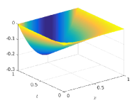
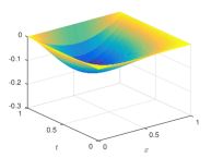
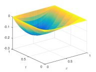
Figure 1. Test 1: Analytical optimal adjoint state $\bar{p}$ (left), POD adjoint solution $p^{\ell}$ utilizing an equidistant time grid with $\Delta t=1/20$ (middle), POD adjoint solution $p^{\ell}$ utilizing an adaptive time grid with dof=21 (right).

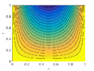
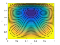
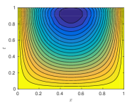
Figure 2. Test 1: Contour lines of the analytical optimal adjoint state $\bar{p}$ (left), POD adjoint solution $p^{\ell}$ utilizing an equidistant time grid with $\Delta t=1/20$ (middle), POD adjoint solution $p^{\ell}$ utilizing an adaptive time grid with dof=21 (right).

In this test run we focus on the influence of the time grid to approximate of the POD solution. Therefore, we compare the use of two different types of time grids: an equidistant time grid characterized by the time increment $\Delta t=1/n$ and a non-equidistant (adaptive) time grid characterized by $n+1$ degrees of freedom (dof). We build the POD-ROM from the uncontrolled problem; we create the snapshot ensemble by determining the associated state $y(u_{\circ})$ and adjoint state $p(u_{\circ})$ corresponding to the control function $u_{\circ}\equiv 0$ and we also include the initial condition $y_{0}$ and the time derivatives of the adjoint $p_{t}(u_{\circ})$ into our snapshot set, which is accomplished with time finite differences of the adjoint snapshots. We use $\ell=1$ POD basis function. Although we would also have the possibility to use suboptimal snapshots corresponding to an approximation $u_{\Delta x}$ of the optimal control, here, we want to emphasize the importance of the time grid. Nevertheless in this example, the quality of the POD solution does not really differ, if we consider suboptimal or uncontrolled snapshots. First, we leave out the post-processing step 4 of Algorithm 1 and discuss the inclusion of this part later.
Figure 3 visualizes the space-time mesh of the numerical solution of (9) utilizing the temporal residual type a-posteriori error estimate (13). The first grid in Figure 3 corresponds to the choice of dof=21 and $\Delta x=1/100$, whereas the grid in the middle refers to using dof = 21 and $\Delta x=1/5$. Both choices for spatial discretization lead to the exact same time grid, which displays fine time steps towards the end of the time horizon (where the layer in the optimal adjoint state is located), whereas at the beginning and in the middle of the time interval the time steps are larger. This clearly indicates that the resulting time adaptive grid is very insensitive against changes in the spatial resolution. For the sake of completeness, the equidistant grid with the same number of degrees of freedom is shown in the right plot of Figure 3.
Since the generation of the time adaptive grid as well as the approximation of the optimal solution is done in the offline computation part of POD-MOR, this process shall be perfomred quickly, which is why we pick $\Delta x=1/5$ for step 1 in Algorithm 1.

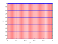
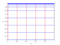
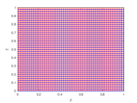
Figure 3. Test 1: Adaptive space-time grids with dof $=21$ according to the strategy in [7] and $\Delta x=1/100$ (left) and $\Delta x=1/5$ (middle), respectively, and the equidistant grid with $\Delta t=1/20$ (right)

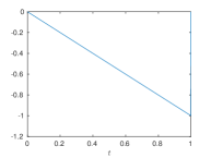
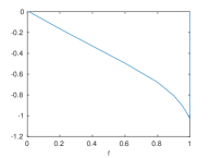
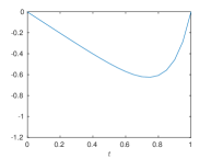
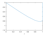
Figure 4. Test 1: Analytical optimal control $\bar{u}$ (top left), approximation $u_{\Delta x}$ of the optimal control gained by step 1 of Algorithm 1 (top right); POD control utilizing a uniform time grid with $\Delta t=1/20$ (bottom left), POD control utilizing an adaptive time grid with dof=21 (bottom right)

Figures 1 and 2 (middle and right plots) show the surface and contour lines of the POD adjoint state utilizing an equidistant time grid and utilizing the time adaptive grid, respectively. The analytical control intensity $\bar{u}(t)$, the approximation $u_{\Delta x}$ of the optimal control computed in step 1 of Algorithm 1 as well as the POD controls utilizing a uniform and time adaptive grid, respectively, are shown in Figure 4.
Table 1 summarizes the approximation quality of the POD solution depending on different time discretizations. The fineness of the time discretization (characterized by $\Delta t$ and dof, respectively) is chosen in such a way that the results of uniform and adaptive temporal discretization are comparable. The absolute errors between the analytical optimal state $\bar{y}$ and the POD solution $y^{\ell}$, defined by $\varepsilon_{\text{abs}}^{y}:=\|\bar{y}-y^{\ell}\|_{L^{2}(\Omega_{T})}$, are listed in columns 2 and 6; same applies for the errors in the control $\varepsilon_{\text{abs}}^{u}:=\|\bar{u}-u^{\ell}\|_{\mathcal{U}}$ (columns 3 and 7) and adjoint state $\varepsilon_{\text{abs}}^{p}:=\|\bar{p}-p^{\ell}\|_{L^{2}(\Omega_{T})}$ (columns 4 and 8). If we compare the results, we note that we gain one order of accuracy for the adjoint and control variable with the time adaptive grid. In order to achieve an accuracy in the control variable of order $10^{-2}$ utilizing an equidistant time grid, we need about $n=10000$ time steps (not listed in Table 1). This emphasizes that using an appropriate (non-equidistant) time grid for the adjoint variable is of particular importance in order to efficiently achieve POD controls of good quality.

$\Delta t$	$\varepsilon_{\text{abs}}^{y}$	$\varepsilon_{\text{abs}}^{u}$	$\varepsilon_{\text{abs}}^{p}$	dof	$\varepsilon_{\text{abs}}^{y}$	$\varepsilon_{\text{abs}}^{u}$	$\varepsilon_{\text{abs}}^{p}$
1/20	$1.5120\cdot 10^{-02}$	$1.9837\cdot 10^{-01}$	$3.6247\cdot 10^{-02}$	21	$5.1874\cdot 10^{-02}$	$5.3428\cdot 10^{-02}$	$9.6343\cdot 10^{-03}$
1/42	$1.1186\cdot 10^{-02}$	$2.1071\cdot 10^{-01}$	$3.8490\cdot 10^{-02}$	43	$5.1634\cdot 10^{-02}$	$2.4868\cdot 10^{-02}$	$4.3611\cdot 10^{-03}$
1/61	$1.0774\cdot 10^{-02}$	$2.1447\cdot 10^{-01}$	$3.9173\cdot 10^{-02}$	62	$5.1599\cdot 10^{-02}$	$2.3275\cdot 10^{-02}$	$4.0691\cdot 10^{-03}$
1/114	$1.1157\cdot 10^{-02}$	$2.1846\cdot 10^{-01}$	$3.9893\cdot 10^{-02}$	115	$5.1568\cdot 10^{-02}$	$2.3027\cdot 10^{-02}$	$4.0340\cdot 10^{-03}$

Table 1. Test 1: Absolute errors between the analytical optimal solution and the POD solution depending on the time discretization (equidistant: columns 1-4, adaptive: columns 5-8)

Table 2 contains the evaluations of each term in (24). The value $\eta_{p}^{i}$ ($\eta_{p}^{b}$) refers to the first (second) part in (13). For this test example, we note that the term $\eta_{p}^{i}$ influences the estimation. However, we observe that the better the semi-discrete adjoint state $p_{\Delta x}$ from step 1 of Algorithm 1 is, the better will be the POD adjoint solution. Since all summands of (24) can be estimated, Table 2 allows us to control the approximation of the POD adjoint state. The estimation (25) concerning the state variable will be investigated later on.

dof	$\varepsilon_{\text{abs}}^{p}$	$\eta_{p}^{i}$	$\eta_{p}^{b}$	$\|\zeta_{k}\|_{U}+\|\zeta_{k}^{\ell}\|_{U}$	$\sum_{i=\ell+1}^{d}\lambda_{i}$
21	$9.6343\cdot 10^{-03}$	$4.9518\cdot 10^{+00}$	$4.8031\cdot 10^{-04}$	$1.6033\cdot 10^{-02}$	$3.3938\cdot 10^{-04}$
43	$4.3611\cdot 10^{-03}$	$1.1976\cdot 10^{+00}$	$5.0087\cdot 10^{-05}$	$1.9200\cdot 10^{-02}$	$2.9454\cdot 10^{-04}$
62	$4.0691\cdot 10^{-03}$	$7.2852\cdot 10^{-01}$	$2.9835\cdot 10^{-05}$	$1.9707\cdot 10^{-02}$	$2.9212\cdot 10^{-04}$
115	$4.0340\cdot 10^{-03}$	$3.4966\cdot 10^{-01}$	$1.4845\cdot 10^{-05}$	$2.0191\cdot 10^{-02}$	$2.9090\cdot 10^{-04}$

Table 2. Test 1: Evaluation of each summand of the error estimation 24

Moreover, a comparison of the value of the cost functional is given in Table 3. The aim of the optimization problem (4) is to minimize the quantity of interest $J(y,u)$. The analytical value of the cost functional at the optimal solution is $J(\bar{y},\bar{u})\approx 8.3988\cdot 10^{+01}$. Table 3 clearly points out that the use of a time adaptive grid is fundamental for solving the optimal control problem (4). The huge differences in the values of the cost functional is due to the great increase of the desired state $y_{d}$ at the end of the time interval (see Figure 5). Small time steps at the end of the time interval, as it is the case in the time adaptive grid, lead to much more accurate results.

$\Delta t$	$J(y^{\ell},u)$	dof	$J(y^{\ell},u)$
1/20	$4.1652\cdot 10^{+04}$	21	$8.7960\cdot 10^{+01}$
1/42	$1.9834\cdot 10^{+04}$	43	$8.4252\cdot 10^{+01}$
1/61	$1.3656\cdot 10^{+04}$	62	$8.4102\cdot 10^{+01}$
1/114	$7.3078\cdot 10^{+03}$	115	$8.4034\cdot 10^{+01}$
1/40000	$8.5692\cdot 10^{+01}$	-	-

Table 3. Test 1: Value of the cost functional at the POD solution utilizing uniform and adaptive time discretization, respectively, analytical value: $J\approx 8.3988\cdot 10^{+01}$

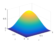
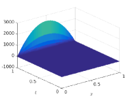
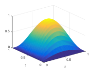
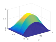
Figure 5. Test 1: Analytical optimal state $\bar{y}$ (top left), desired state $y_{d}$ (top right); POD state $y^{\ell}$ utilizing a uniform time grid with $\Delta t=1/20$ (bottom left), POD state $y^{\ell}$ utilizing an adaptive time grid with dof = 21 (bottom right)

Now, let us discuss the inclusion of step 4 in Algorithm 1. Since we went for an adaptive time grid regarding the adjoint variable, we cannot in general expect that the resulting time grid is a good time grid for the state variable. Table 1 confirms that utilizing a uniform time grid leads to better approximation results in the state variable than using the time adaptive grid. In order to improve also the approximation quality in the state variable, we incorporate the error estimation (25) from [17] in a post-processing step after producing the time grid with the strategy of [7] and before starting the POD solution process. Define

$\eta_{\text{POD}_{j}}:=\Delta t_{j}^{2}\left(\int\limits_{I_{j}}(\|y_{tt}^{k}\|_{H}^{2}+\|y_{t}^{k}\|_{V}^{2})\right)$

where $y_{t}^{k}\approx y_{t}(t_{k})$ and $y_{tt}^{k}\approx y_{tt}(t_{k})$ are computed via finite difference approximation. We perform bisection on those time intervals $I_{j}$, where the quantity $\eta_{\text{POD}_{j}}$ has its maximum value and repeat this $N_{\text{refine}}$ times. This results in the time grid $\mathcal{T_{\text{new}}}$. The improvement in the approximation quality in the state variable can be seen in Table 4. The more additional time instances we include according to (25), the better the approximation results get with respect to the state. Moreover, also the approximation quality in the control and adjoint state is improved.

$N_{\text{refine}}$	$\varepsilon_{\text{abs}}^{y}$	$\varepsilon_{\text{abs}}^{u}$	$\varepsilon_{\text{abs}}^{p}$
0	$5.1874\cdot 10^{-02}$	$5.3428\cdot 10^{-02}$	$9.6343\cdot 10^{-03}$
5	$4.0058\cdot 10^{-02}$	$2.1145\cdot 10^{-02}$	$3.6378\cdot 10^{-03}$
10	$3.0909\cdot 10^{-02}$	$1.8396\cdot 10^{-02}$	$3.0895\cdot 10^{-03}$
20	$2.4759\cdot 10^{-02}$	$1.7104\cdot 10^{-02}$	$2.8210\cdot 10^{-03}$
30	$2.3028\cdot 10^{-02}$	$1.6971\cdot 10^{-02}$	$2.7906\cdot 10^{-03}$

Table 4. Test 1: Improvement of approximation quality concerning the state variable. The initial time grid $\mathcal{T}$ is computed with dof=43

We note that the sum of the neglected eigenvalues $\sum_{i=2}^{d}\lambda_{i}$ is approximately zero and the second largest eigenvalue of the correlation matrix is of order $10^{-10}$, which makes the use of additional POD basis functions redundant. Likewise, in this particular example the choice of richer snapshots (even the optimal snapshots) does not bring significant improvements in the approximation quality of the POD solutions. So, this example shows that solely the use of an appropriate adaptive time mesh efficiently improves the accuracy of the POD solution.

6.2. Test 2: Solution with steep gradient in the middle of the time interval

Let $\Omega=(0,1)$ be the spatial domain and $[0,T]=[0,1]$ be the time interval. We choose $\varepsilon=10^{-4}$ and $\alpha=1$. To begin with, we consider an unconstrained optimal control problem and investigate the inclusion of control constraints separately in Test 3. We build the example in such a way that the analytical solution $(\bar{y},\bar{u})$ of (4) is given by:

$$\bar{y}(x,t)=x^{3}(x-1)t,\quad\bar{p}(x,t)=\sin(\pi x)\text{atan}\left(\frac{t-0.5}{\varepsilon}\right)(t-1),$$

$$\bar{u}_{1}(t)=\bar{u}_{2}(t)=-\text{atan}\left(\frac{t-0.5}{\varepsilon}\right)(t-1)\left(\frac{32}{\pi^{3}}-\frac{8}{\pi^{2}}\right),$$

$$\bar{\chi}_{1}(x)=\max(0,1-16(x-0.25)^{2}),\quad\bar{\chi}_{2}(x)=\max(0,1-16(x-0.75)^{2}).$$

The desired state and the forcing term are chosen accordingly. Due to the arcus-tangens term and the small value for $\varepsilon$, the adjoint state exhibits an interior layer with steep gradient at $t=0.5$, which can be seen in the left panel of Figure 6 and 7. The shape functions $\chi_{1}$ and $\chi_{2}$ are shown in Figure 8 on the left side. Like in Test 1, we study the use of two different time grids: an equidistant time discretization and the time adaptive grid computed in step 1 of Algorithm 1 (see Figure 9). Once again, we note that spatial and temporal discretization decouple when computing the time adaptive grid utilizing the a-posteriori estimation (13), which enables us to use a large spatial resolution $\Delta x$ for solving the elliptic system and to keep the offline costs low.

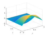
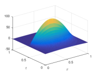
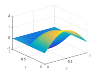
Figure 6. Test 2: Analytical optimal adjoint state $\bar{p}$ (left), POD adjoint solution $p^{\ell}$ with $\ell=4$ utilizing an equidistant time grid with $\Delta t=1/40$ (middle), POD adjoint solution $p^{\ell}$ with $\ell=4$ utilizing an adaptive time grid with dof=41 (right)

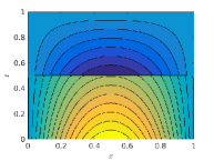
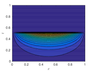
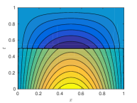
Figure 7. Test 2: Contour lines of the analytical optimal adjoint state $\bar{p}$ (left), POD adjoint solution $p^{\ell}$ with $\ell=4$ utilizing an equidistant time grid with $\Delta t=1/40$ (middle), POD adjoint solution $p^{\ell}$ with $\ell=4$ utilizing an adaptive time grid with dof=41 (right)

As snaphots, we choose state and adjoint snapshots as well as time derivative adjoint snapshots corresponding to $u_{\circ}=0$ and we also include the initial condition $y_{0}$ into our snapshot set. The middle and right plots of Figures 6 and 7 show the surface and contour lines of the POD adjoint solution utilizing an equidistant time grid (with $\Delta t=1/40$) and utilizing the adaptive time grid (with dof = 41), respectively. Clearly, the equidistant time grid fails to capture the interior layer at $t=1/2$ satisfactorily, whereas the POD adjoint state utilizing the adaptive time grid approximates the interior layer well.

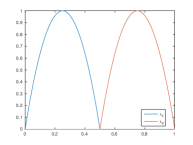
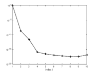
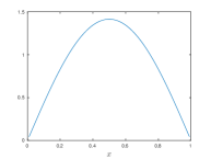
Figure 8. Test 2: Shape functions $\chi_{1}(x)$ and $\chi_{2}(x)$ (left), decay of the eigenvalues on semilog scale (middle) and first POD basis function $\psi_{1}$ (right) utilizing uniform time grid with $\Delta t=1/40$

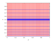
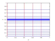
Figure 9. Test 2: Adaptive space-time grids with dof $=41$ according to the strategy in [7] and $\Delta x=1/100$ (left) and $\Delta x=1/5$ (middle), respectively, and the equidistant grid with $\Delta t=1/40$ (right)

Unlike Test Example 6.1, the adaptive time grid is also a suitable time grid for the state variable in this numerical test example. This can be seen visually when comparing the results for the POD state utilizing uniform discretization and utilizing the adaptive time grid with the analytical optimal state, Figures 10 and 11.

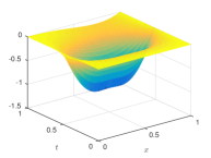
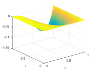
Figure 10. Test 6.2: Analytical optimal state $\bar{y}$ (left), POD solution $y^{\ell}$ with $\ell=4$ utilizing an equidistant time grid with $\Delta t=1/40$ (middle), POD solution $y^{\ell}$ with $\ell=4$ utilizing an adaptive time grid with dof=41 (right)

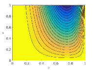
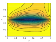
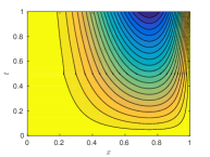
Figure 11. Test 6.2: Contour lines of the analytical optimal state $\bar{y}$ (left), POD solution $y^{\ell}$ with $\ell=4$ utilizing an equidistant time grid with $\Delta t=1/40$ (middle), POD solution $y^{\ell}$ with $\ell=4$ utilizing an adaptive time grid with dof=41 (right)

Table 5 summarizes the absolute errors between the analytical optimal solution and the POD solution for the state, control and adjoint state for all test runs with an equidistant and adaptive time grid, respectively. If we compare the results of the numerical approximation, we note that the use of an adaptive time grid heavily improves the quality of the POD solution with respect to an equidistant grid. In fact, we get an improvement up to order four.

$\Delta t$	$\varepsilon_{\text{abs}}^{y}$	$\varepsilon_{\text{abs}}^{u}$	$\varepsilon_{\text{abs}}^{p}$	dof	$\varepsilon_{\text{abs}}^{y}$	$\varepsilon_{\text{abs}}^{u}$	$\varepsilon_{\text{abs}}^{p}$
1/20	$5.0767\cdot 10^{-01}$	$7.8419\cdot 10^{+00}$	$3.5413\cdot 10^{+01}$	21	$4.0346\cdot 10^{-02}$	$5.4053\cdot 10^{-01}$	$2.4409\cdot 10^{+00}$
1/40	$2.6242\cdot 10^{-01}$	$4.1058\cdot 10^{+00}$	$1.8542\cdot 10^{+01}$	41	$2.2178\cdot 10^{-04}$	$5.3471\cdot 10^{-03}$	$1.3186\cdot 10^{-02}$
1/68	$1.5603\cdot 10^{-01}$	$2.4503\cdot 10^{+00}$	$1.1065\cdot 10^{+01}$	69	$9.7031\cdot 10^{-05}$	$4.5702\cdot 10^{-03}$	$4.2670\cdot 10^{-03}$
1/134	$7.8741\cdot 10^{-02}$	$1.2386\cdot 10^{+00}$	$5.5938\cdot 10^{+00}$	135	$8.5577\cdot 10^{-05}$	$4.4901\cdot 10^{-03}$	$2.3507\cdot 10^{-03}$

Table 5. Test 6.2: Absolute errors between the analytical optimal solution and the POD solution with $\ell=4$ depending on the time discretization (equidistant: columns 1-4, adaptive: columns 5-8)

The exact optimal control intensities $\bar{u}_{1}(t)$ and $\bar{u}_{2}(t)$ as well as the POD solutions utilizing uniform and adaptive temporal discretization are illustrated in Figure 12.
Another point of comparison is the evaluation of the cost functional. Since the exact optimal solution is known analytically, we can compute the exact value of the cost functional, which is $J(\bar{y},\bar{u})=1.0085\cdot 10^{+03}$. As expected, utilizing an adaptive time grid enables us to approximate this value of the cost functional quite well when using dof=135, see Table 6. In contrast, the use of a very fine temporal discretization with $\Delta t=1/10000$ is still worse than the results with the adaptive time grid and dof $\geq 41$. Again, this emphasizes the importance of a suitable time grid.

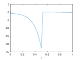
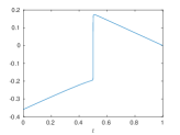
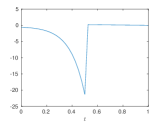
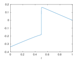
Figure 12. Test 2: Analytical control intensities $\bar{u}_{1}(t)$ (top left) and $\bar{u}_{2}(t)$ (bottom left), POD control utilizing an equidistant time grid with $\Delta t=1/40$ (middle) and $\ell=4$, POD control utilizing an adaptive time grid with dof=41 (right) and $\ell=4$

$\Delta t$	$J(y^{\ell},u)$	dof	$J(y^{\ell},u)$
1/20	$3.1225\cdot 10^{+05}$	21	$1.9553\cdot 10^{+04}$
1/40	$1.5619\cdot 10^{+05}$	41	$1.0274\cdot 10^{+03}$
1/68	$9.1901\cdot 10^{+04}$	69	$1.0065\cdot 10^{+03}$
1/134	$4.6655\cdot 10^{+04}$	135	$1.0082\cdot 10^{+03}$
1/10000	$1.0350\cdot 10^{+03}$	–	–

Table 6. Test 2: Value of the cost functional with $\ell=4$, true value $J\approx 1.0085\cdot 10^{+03}$

Now, we like to investigate which influence the number $\ell$ of utilized POD basis functions has on the approximation quality of the POD solution. First, we have a look at the decay of the eigenvalues, which is displayed in Figure 8, middle. The eigenvalues stagnate nearby the order of machine precision, which is why the use of more than $\ell=4$ POD basis functions will not lead to better POD approximation results. The first POD basis function $\psi_{1}$ can be seen in the right plot of Figure 8. For the use of only $\ell=1$ POD basis function, the absolute error between the analytical solution and the POD solution in the state, control and adjoint state for uniform as well as for adaptive time discretization are summarized in Table 7. Let us compare the results in this Table 7 where $\ell=1$ POD basis function is used with the results in Table 5 where $\ell=4$ POD basis functions are used. We note that in the case of the uniform temporal discretization, the use of $\ell=1$ POD basis function leads to similar approximation results like when using $\ell=4$ POD modes. On the contrary, in the case of the adaptive time discretization, the use $\ell=4$ POD basis functions leads to better approximation results with respect to the state variable than using $\ell=1$ POD basis. The approximation results concerning the control and adjoint state differ only slightly when increasing the number of utilized POD basis functions. Nevertheless, also for the use of only $\ell=1$ POD mode, the use of the time adaptive grid leads to an improvement of the absolute errors of up to four decimal points in comparison to using a uniform time grid.

$\Delta t$	$\varepsilon_{\text{abs}}^{y}$	$\varepsilon_{\text{abs}}^{u}$	$\varepsilon_{\text{abs}}^{p}$	dof	$\varepsilon_{\text{abs}}^{y}$	$\varepsilon_{\text{abs}}^{u}$	$\varepsilon_{\text{abs}}^{p}$
1/20	$5.0631\cdot 10^{-01}$	$7.8420\cdot 10^{+00}$	$3.5413\cdot 10^{+01}$	21	$4.5255\cdot 10^{-02}$	$5.4054\cdot 10^{-01}$	$2.4409\cdot 10^{+00}$
1/40	$2.6230\cdot 10^{-01}$	$4.1059\cdot 10^{+00}$	$1.8542\cdot 10^{+01}$	41	$2.0721\cdot 10^{-02}$	$5.3475\cdot 10^{-03}$	$1.3186\cdot 10^{-02}$
1/68	$1.5684\cdot 10^{-01}$	$2.4503\cdot 10^{+00}$	$1.1065\cdot 10^{+01}$	69	$2.0713\cdot 10^{-02}$	$4.5706\cdot 10^{-03}$	$4.2670\cdot 10^{-03}$
1/134	$8.1129\cdot 10^{-02}$	$1.2386\cdot 10^{+00}$	$5.5938\cdot 10^{+00}$	135	$2.0664\cdot 10^{-02}$	$4.4905\cdot 10^{-03}$	$2.3507\cdot 10^{-03}$

Table 7. Test 2: Absolute errors between the analytical optimal solution and the POD solution with $\ell=1$ depending on the time discretization (equidistant: columns 1-4, adaptive: columns 5-8)

6.3. Test 3: Control constrained problem

In this test we add control constraints to the previous example. We set $u_{1,a}(t)\leq u_{1}(t)\leq u_{1,b}(t)$ and $u_{2,a}(t)\leq u_{2}(t)\leq u_{2,b}(t)$ for the time dependent control intensities $u_{1}(t)$ and $u_{2}(t)$. The analytical value range for both controls is $u_{1}(t),u_{2}(t)\in[-0.3479,0.1700]$ for $t\in[0,1]$. For each control intensity we choose different upper and lower bounds: we set $u_{1,a}(t)=-100$ (i.e. no restriction), $u_{1,b}=0.1$ and $u_{2,a}(t)=-0.2,\;u_{2,b}(t)=0$. For the solution of problem (19) we use a projected gradient method.

The solution of the nonlinear, nonsmooth equation (9) can be done by a semi-smooth Newton method or by a Newton method utilizing a regularization of the projection formula, see [21]. In our numerical tests we compute the approximate solution to (19) with a fixed point iteration and initialize the method with the adjoint state corresponding to the control unconstrained optimal control problem. In this way, only two iterations are needed for convergence. Convergence of the fixed point iteration can be argued for large enough values of $\alpha$, see [11].
The analytical optimal solutions $\bar{u}_{1}$ and $\bar{u}_{2}$ are shown in the left plots in Figure 13. For POD basis computation, we use state, adjoint and time derivative adjoint snapshots corresponding to the reference control $u_{\circ}=0$ and we also include the initial condition $y_{0}$ into our snapshot set. The plots in the middle and on the right in Figure 13 refer to the POD controls using a uniform and an adaptive temporal discretization, respectively. Once again, we note that utilizing an adaptive time grid leads to far better results than using a uniform temporal grid. The numerical results in Table 8 confirm this observation. We observe that the inclusion of box constraints on the control functions lead in general to better approximation results, compare Table 5 with Table 8. This is due to the fact that on the active sets the error between the analytical optimal controls and the POD solutions vanishes.

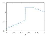
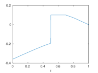
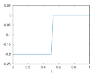
Figure 13. Test 3: Inclusion of box constraints for the control intensities: Analytical control intensities $\bar{u}_{1}(t)$ (top left) and $\bar{u}_{2}(t)$ (bottom left), POD control utilizing an equidistant time grid with $\Delta t=1/40$ (middle) and $\ell=4$, POD control utilizing an adaptive time grid with dof=41 (right) and $\ell=4$

$\Delta t$	$\varepsilon_{\text{abs}}^{y}$	$\varepsilon_{\text{abs}}^{u}$	$\varepsilon_{\text{abs}}^{p}$	dof	$\varepsilon_{\text{abs}}^{y}$	$\varepsilon_{\text{abs}}^{u}$	$\varepsilon_{\text{abs}}^{p}$
1/20	$2.8601\cdot 10^{-01}$	$5.7201\cdot 10^{+00}$	$3.5430\cdot 10^{+01}$	21	$2.2714\cdot 10^{-02}$	$3.9586\cdot 10^{-01}$	$2.4423\cdot 10^{+00}$
1/40	$1.4802\cdot 10^{-01}$	$2.9955\cdot 10^{+00}$	$1.8551\cdot 10^{+01}$	41	$2.9482\cdot 10^{-04}$	$4.4969\cdot 10^{-03}$	$1.3183\cdot 10^{-02}$
1/68	$8.8124\cdot 10^{-02}$	$1.7882\cdot 10^{+00}$	$1.1071\cdot 10^{+01}$	69	$2.1247\cdot 10^{-04}$	$3.2811\cdot 10^{-03}$	$4.2629\cdot 10^{-03}$
1/134	$4.4570\cdot 10^{-02}$	$9.0470\cdot 10^{-01}$	$5.5965\cdot 10^{+00}$	135	$2.1330\cdot 10^{-04}$	$3.1321\cdot 10^{-03}$	$2.3474\cdot 10^{-03}$

Table 8. Test 3: Inclusion of box constraints for the control intensities: Absolute errors between the analytical optimal solution and the POD solution with $\ell=4$ depending on the time discretization (equidistant: columns 1-4, adaptive: columns 5-8)

7. Conclusion

In this paper we investigated the problem of snapshot location in optimal control problems. We showed that the numerical POD solution is much more accurate if we use an adaptive time grid, especially when the solution of the problem presents steep gradients. The time grid was computed by means of an a-posteriori error estimation strategy of space-time approximation of a second order in time and fourth order in space elliptic equation which describes the optimal control problem and has the advantage that it is independent of an input control function. Furthermore, a coarse approximation with respect to space of the latter equation gives information on the snapshots one can use to build the surrogate model. Finally, we provided a certification of our surrogate model by means of an a-posteriori error estimation for the error between the optimal solution and the POD solution.
For future work, we are interested in transferring our approach to optimal control problems subject to nonlinear parabolic equations.

References

- [1] K. Afanasiev and M. Hinze. Adaptive control of a wake flow using proper orthogonal decomposition. Lecture Notes in Pure and Applied Mathematics 216, 317-332. Shape Optimization & Optimal Design, Marcel Dekker, 2001.
- [2] A. Alla and M. Falcone. An adaptive POD approximation method for the control of advection-diffusion equations International Series of Numerical Mathematics (Birkhauser, Basel, 2013)
- [3] A. Alla, C. Gräßle and M. Hinze. A residual based snapshot location strategy for POD in distributed optimal control of linear parabolic equations, submitted, 2015.
- [4] E. Arian, M. Fahl and E. Sachs. Trust-region proper orthogonal decomposition models by optimization methods. In Proceedings of the 41st IEEE Conference on Decision and Control, Las Vegas, Nevada, 2002, 3300-3305.
- [5] L. C. Evans. Partial Differential Equations. Graduate Studies in Mathematics, 19, American Mathematical Society, Providence, RI, 2010.
- [6] J. Ghiglieri and S. Ulbrich. Optimal Flow Control Based on POD and MPC and an Application to the Cancellation of Tollmien-Schlichting Waves. Optimization Methods and Software, 29 (2014), 1042-1074.
- [7] W. Gong, M. Hinze and Z.J.Zhou. Space-time finite element approximation of parabolic optimal control problems J. Numer. Math, 20, 2012, 111-145.
- [8] M. Gubisch and S. Volkwein. Proper Orthogonal Decomposition for Linear-Quadratic Optimal Control. Submitted, 2013.
- [9] M. Hinze. A variational discretization concept in control constrained optimization: the linear-quadratic case. Computational Optimization and Applications, 30, 2005, 45-61.
- [10] M. Hinze, R. Pinnau, M. Ulbrich and S. Ulbrich. Optimization with PDE Constraints. Mathematical Modelling: Theory and Applications, 23. Springer Verlag, 2009.
- [11] M. Hinze and M. Vierling. Variational discretization and semi-smooth Newton methods; implementation, convergence and globalization in pde constrained optimzation with control constraints. Optim. Meth. Software 27, 2012, 933-950.
- [12] M. Hinze and S. Volkwein. Error estimates for abstract linear-quadratic optimal control problems using proper orthogonal decomposition. S. Comput. Optim. Appl. 39, 2008, 319-345.
- [13] R.H.W. Hoppe and Z. Liu. Snapshot location by error equilibration in proper orthogonal decomposition for linear and semilinear parabolic partial differential equations Journal of Numerical Mathematics, 22, 2014, 1-32.
- [14] E. Kammann, F. Tröltzsch and S. Volkwein. A method of a-posteriori error estimation with application to proper orthogonal decomposition ESAIM: M2AN, 47, 2013, 555-581.
- [15] Z. Kanar Seymen, H. Yücel and B. Karasözen. Distributed optimal control of time-dependent diffusion-convection-reaction equations using space-time discretization Journal of Computational and Applied Mathematics, 261, 2014, 146-157.
- [16] K. Kunisch and S. Volkwein. Galerkin proper orthogonal decomposition methods for parabolic problems. Numer. Math. 90, 2001, 117-148.
- [17] K. Kunisch and S. Volkwein. Galerkin proper orthogonal decomposition methods for a general equation in fluid dynamics. SIAM, J. Numer. Anal. 40, 2002, 492-515.
- [18] K. Kunisch and S. Volkwein. Proper Orthogonal decomposition for optimality systems ESAIM: M2AN, 42, 2008, 1-23.
- [19] K. Kunisch and S. Volkwein. Optimal Snapshot Location for computing POD basis functions ESAIM: M2AN, 44, 2010, 509-529.
- [20] J.L. Lions. Optimal Control of Systems Governed by Partial Differential Equations Grundlehren der mathematischen Wissenschaften, Springer, 1971.
- [21] I. Neitzel, U. Prüfert and T. Slawig. A Smooth Regularization of the Projection Formula for Constrained Parabolic Optimal Control Problems Numerical Functional Analysis and Optimization 32, 2011, 1283-1315.
- [22] I. Neitzel and B. Vexler. A priori error estimates for space-time finite element discretization of semilinear parabolic optimal control problems Numerische Mathematik 120, 2012, 345-386.
- [23] J. Nocedal and S.J. Wright. Numerical Optimization, second edition. Springer Series in Operation Research, 2006.
- [24] N.C. Nguyen, G. Rozza and A.T. Patera. Reduced basis approximation and a posteriori error estimation for time dependent viscous Burgers equation. Calcolo, 46, 2009, 157-185.
- [25] G.M. Oxberry, T. Kostova-Vassilevska, B. Arrighi and K. Chand. Limited-memory adaptive snapshot selection for proper orthogonal decomposition. Preprints, 2015.
- [26] A. T. Patera and G. Rozza. Reduced Basis Approximation and A Posteriori Error Estimation for Paramtrized Partial Differential Equations. MIT Pappalardo Graduate Monographs in Mechanical Engineering, 2006.
- [27] G. Rozza, D.B.P. Huynh and A.T. Patera. Reduced Basis Approximation and a Posteriori Error Estimation for Affinely Parametrized Elliptic Coercive Partial Differential Equations. Arch. Comput. Methods. Eng., 15, 2008, 229-275.
- [28] L. Sirovich. Turbulence and the dynamics of coherent structures. Parts I-II, Quarterly of Applied Mathematics, XVL, 1987, 561-590.
- [29] F. Tröltzsch. Optimal Control of Partial Differential Equations: Theory, Methods and Application, American Mathematical Society, 2010.
- [30] F. Tröltzsch and S. Volkwein. POD a-posteriori error estimates for linear-quadratic optimal control problems Computational Optimization and Applications, 44, 2009, 83-115.
- [31] S. Volkwein and A. Studinger. Numerical analysis of POD a-posteriori error estimation for optimal control International Series of Numerical Mathematics (Birkhauser, Basel, 2013)
- [32] S. Volkwein. Optimality system POD and a-posteriori error analysis for linear-quadratic problems Control and Cybernetics, 40, 2011, 1109-1125.