KUNS-2640
Possible explanations for fine-tuning of the universe

Abstract

The Froggatt-Nielsen mechanism and the multi-local field theory are interesting and promising candidates for solving the naturalness problem in the universe. These theories are based on the different physical principles: The former assumes the micro-canonical partition function $\int{\cal{D}}\phi\ \prod_{i}\delta(S_{i}-I_{i})$, and the latter assumes the partition function $\int{\cal{D}}\phi\ \exp\left(iS_{M}\right)$ where $S_{M}$ is the multi-local action $\sum_{i}c_{i}S_{i}+\sum_{i,j}c_{i,j}S_{i}S_{j}+\cdots$. Our main purpose is to show that they are equivalent in the sense that they predict the same fine-tuning mechanism. In order to clarify our argument, we first study (review) the similarity between the Froggatt-Nielsen mechanism and statistical mechanics in detail, and show that the dynamical fine-tuning in the former picture can be understood completely in the same way as the determination of the temperature in the latter picture. Afterward, we discuss the multi-local theory and the equivalence between it and the the Froggatt-Nielsen mechanism. Because the multi-local field theory can be obtained from physics at the Planck/String scale, this equivalence indicates that the micro-canonical picture can also originate in such physics. As a concrete example, we also review the IIB matrix model as an origin of the multi-local theory.

Although the Standard Model (SM) is completed by the discovery of the Higgs boson, there are many open questions in it such as the Higgs quadratic divergence, the Strong CP problem, the cosmological constant problem, and so on. These problems are difficult to answer in ordinary quantum field theory (QFT), and called the naturalness problem. Therefore, it is quite important to seek for new theory or mechanism that naturally answers these questions.

One of the possibilities is to try to explain the observed couplings by dynamical fine-tuning. For example, in the Strong CP problem, $\theta$ becomes dynamical by considering the Peccei-Quinn symmetry and its breaking. However, even if such a field theoretical approach with a new symmetry can solve one of the fine-tunings, it is difficult to solve a few problems simultaneously. So, it is meaningful to study new mechanism that can realize a few fine-tunings simultaneously.

Among various proposals, the Froggatt-Niselsen mechanism (FNM) [1] recently attracts much attention because the predicted value of the Higgs mass ($\sim 130$GeV) was close to the observed value $\simeq 125$GeV. It was originally proposed to explain the nontrivial behavior of the SM Higgs potential at high energy scale: The potential has another minimum around the Planck scale, and it can degenerate with the electroweak vacuum $v_{h}=246$GeV depending on the values of the SM couplings. Such a degeneration is called the Multiple point criticality principle (MPP), and there are a lot of studies so far [2]. The fundamental assumption in the FNM is to use the micro-canonical partition function like statistical mechanics, and its origin still remains obscure. In this picture, the couplings in QFT become dynamical, and their dynamical fine-tuning can take place. See [1, 2] and the following discussion for the details.

On the other hand, in [3], it was also argued that a few naturalness problems, including the MPP, can be solved by the multi-local field theory. It assumes that the effective action below the Planck/String scale is given by the multi-local one: $\sum_{i}c_{i}S_{i}+\sum_{i,j}c_{i,j}S_{i}S_{j}+\cdots$, where $S_{i}$’s are ordinary actions, and $c_{i}$’s, $c_{ij}$’s, $\cdots$ are constants. Although it seems difficult to study the theory as quantum theory, we will see that we can reduce it to QFT with the couplings being dynamical by a simple mathematical transformation. See the following discussion for the details. As well as the FNM, we do not need to consider its fundamental origin as long as we apply it to the naturalness problem, however, such an origin can be actually found in physics at the Planck/String scale. Therefore, the multi-local theory seems to be more promising than the FNM it that everything can be explained from more fundamental physics.

The purpose of this paper is to show that these two approaches are in fact equivalent in the sense that they predict the same fine-tuning mechanism in QFT: The coupling in QFT is fixed at the point that most strongly dominates in their partition functions, and the fine-tuned value generally depends on the details of the theories. This fact indicates that the micro-canonical picture may also originate in the Planck/String scale physics such as the wormhole theory [4] or matrix model. As a concrete example, we also review the derivation of the multi-local theory from the IIB matrix model [5]. Although the study in [5] is mathematically rigorous, most of the discussion can be done without relying on the details of mathematics. So, in this paper, we aim to give an instructive and intuitive explanation of their work.

Let us first review the FNM. In ordinary QFT, a system is completely described by the partition function:

$$Z^{\text{(QFT)}}(\lambda)=\int{\cal{D}}\phi\ \exp\left(iS\right),$$ (1)

where $S$ is a given action, and $\lambda$ represents a coupling in $S$. The corresponding quantity in statistical mechanics is the canonical distribution:

$$Z_{\text{C}}^{(\text{Statistical})}(\beta)=\sum_{n}\exp\left(-\beta E_{n}\right),$$ (2)

where $\beta=1/T$ is the inverse temperature, and $E_{n}$’s are the energy eigenvalues. On the other hand, it is known that this distribution is equivalent to the micro-canonical distribution

$$Z_{\text{MC}}^{(\text{Statistical})}(E)=i\pi\sum_{n}\delta(E_{n}-E)$$ (3)

in the thermodynamic limit . Here, we have added the overall coefficient $i\pi$ just for the following argument. From the microscopic point of view, the micro-canonical distribution is more fundamental because there is no thermodynamical quantity in Eq.(3). In this picture, the temperature $T$ is dynamically determined by the following way: Eq.(3) can be rewritten as

$$=\sum_{n}\left[\frac{1}{E_{n}-E}-P\left(\frac{1}{E_{n}-E}\right)\right]$$

$$=\int_{0}^{\infty}d\beta\ \sum_{n}\exp\left(-\beta(E_{n}-E)\right)-\sum_{n}P\left(\frac{1}{E_{n}-E}\right)$$

$$\simeq\int_{0}^{\infty}d\beta\ Z^{(\text{Statistical})}_{\text{C}}(\beta)e^{\beta E}=\int_{0}^{\infty}d\beta\ \exp\left(-\beta(F(\beta)-E)\right),$$ (6)

where $P$ represents the Cauchy principal value, and $F(\beta)$ is the free energy. In the thermodynamic limit, this integral is dominated by $\beta^{*}(E)=1/T^{*}(E)$ that satisfies

$$\frac{\partial}{\partial\beta}\left(\beta F(\beta)\right)\bigg{|}_{\beta=\beta^{*}}-E=0\ \leftrightarrow\ \langle H\rangle_{\text{C}}=E,$$ (7)

where $H$ is the Hamiltonian of the system, and $\langle\ \rangle_{\text{C}}$ represents the average by the canonical distribution. Thus, $T$ is dynamically fixed so that the average of $H$ by the canonical distribution can become $E$, and its value depends on $E$. Although E is completely arbitrary from the microscopic point of view, there is a special interval where $T^{*}(E)$ does not depend on $E$: coexisting of different phases. See Fig.1 for example. This figure shows a schematic contour of $T^{*}(E)$. When different phases coexist, $T^{*}(E)=T_{\text{cri}}$ does not change until the system gains enough energy. From the naturalness point of view, this fact indicates that $T$ is most likely to be fixed at the critical value $T_{\text{cri}}$ because the probability of $E$ being chosen to be in the interval is biggest. In the following, we will apply the above argument to QFT, and see that the coupling in QFT corresponds to $T$ in statistical mechanics.

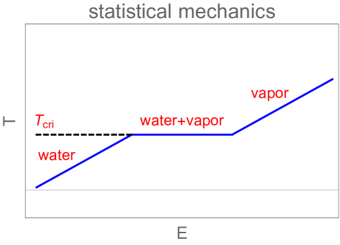
Figure 1: The blue contour shows $T^{*}(E)$ determined by the micro-canonical distribution. For example, consider water heated by external environment. While the phase transition occurs, $T^{*}(E)$ does not change.

By considering the above discussion, it is natural to adopt the micro-canonical partition function even in QFT:

$$Z^{\text{(QFT)}}_{\text{MC}}=\int{\cal{D}}\phi\ \prod_{i}\delta(S_{i}-I_{i}),$$ (8)

where $S_{i}$’s are the ordinary local actions in QFT, and $I_{i}$’s are their arbitrary values. In principle, $S_{i}$’s in Eq.(8) should be determined from the microscopic physics such as String theory . Note that $I_{i}$’s correspond to $E$ in statistical mechanics. Rewriting the delta function in Eq.(8) as the Fourier form, we obtain

$$Z^{\text{(QFT)}}_{\text{MC}} =\int{\cal{D}}\phi\ \int\cdots\int\left(\prod_{i}d\lambda_{i}\right)\ \exp\left(i\sum_{i}\lambda_{i}(S_{i}-I_{i})\right)$$

$$=\int\cdots\int\left(\prod_{i}d\lambda_{i}\right)\ Z^{(\text{QFT})}(\overrightarrow{\lambda})=\int\cdots\int\left(\prod_{i}d\lambda_{i}\right)\ \exp\left(-iV_{4}\rho(\overrightarrow{\lambda})\right),$$ (9)

where we have introduced the Lagrange multipliers $\lambda_{i}$’s, and $\rho(\overrightarrow{\lambda})$ is the vacuum energy density. One can see that $\lambda_{i}$’s play roles of the couplings. Thus, if there is a point $\overrightarrow{\lambda}_{0}$ that strongly dominates in the above integration, we have

$$\sim Z^{(\text{QFT})}(\overrightarrow{\lambda}_{0}),$$ (10)

and this is the ordinary partition function where $\overrightarrow{\lambda}$ is fixed to $\overrightarrow{\lambda}_{0}$. Here, note that such a dominant point is naively given by the saddle point of $\rho(\overrightarrow{\lambda})$ :

$$\frac{\partial\rho(\overrightarrow{\lambda})}{\partial\lambda_{i}}=\frac{\int{\cal{D}}\phi\ (S_{i}-I_{i})\exp\left(i\sum_{j}\lambda_{j}(S_{j}-I_{j})\right)}{Z^{(\text{QFT})}(\overrightarrow{\lambda})}=\langle S_{i}\rangle-I_{i}=0.$$ (11)

In [1], Froggatt and Nielsen showed that, for the wide range of $I_{i}$, the above saddle point corresponds to the coexisting phase of the Higgs vacua like the phase transition in statistical mechanics. As one of examples, let us choose the Higgs quartic term $S_{H}=\int d^{4}x\ \left(H^{\dagger}H\right)^{2}$ as $S_{i}$, and confirm their claim. Because the Higgs potential can have two minima depending on the couplings in the SM, we denote the small (large) vacuum expectation value as $\phi_{1}(\lambda)$ ($\phi_{2}(\lambda)$) in the following discussion. Furthermore, we represent the critical Higgs quartic coupling where the two vacua degenerate as $\lambda_{\text{cri}}$. When $I_{H}\leq\phi_{1}(\lambda_{\text{cri}})^{4}V_{4}\ (V_{4}:\text{spacetime volume})$, the Higgs quartic coupling $\lambda$ is fixed at the point $\lambda^{*}(I_{H})\ (\geq\lambda_{\text{cri}})$ so that $\phi_{1}(\lambda)$ can satisfy Eq.(11):

$$\langle S_{H}\rangle=\phi_{1}(\lambda^{*}(I_{H}))^{4}V_{4}=I_{H}.$$ (12)

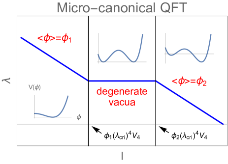
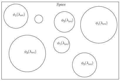
Figure 2: Left: The fixed Higgs quartic coupling $\lambda$ as a function of $I_{H}$. As well as the statistical mechanics, there is a finite interval $\phi_{1}(\lambda_{\text{cri}})^{4}V_{4}\leq I_{H}\leq\phi_{2}(\lambda_{\text{cri}})^{4}V_{4}$ where the phase coexisting is realized. Right: The coexisting of the Higgs vacua when $\phi_{1}(\lambda_{\text{cri}})^{4}V_{4}\leq I_{H}\leq\phi_{2}(\lambda_{\text{cri}})^{4}V_{4}$.

In the left panel in Fig.2, we show $\lambda^{*}(I_{H})$ by a blue contour. Note that $\phi_{1}(\lambda)$ is the true vacuum in the this case. As we increase $I_{H}$, $\lambda^{*}(I_{H})$ decreases in order to satisfy Eq.(12). When $I_{H}$ becomes $\phi_{1}(\lambda_{\text{cri}})^{4}V_{4}$, namely, $\lambda^{*}(I_{H})$ becomes $\lambda_{\text{cri}}$, the system undergoes the first order phase transition. At first glance, it seems difficult to find the solution of Eq.(11) because $\langle S_{H}\rangle$ changes discretely at that point. However, even if $I_{H}>\phi_{1}(\lambda_{\text{cri}})^{4}V_{4}$, the universe can actually satisfy Eq.(11) by keeping the coexisting of two vacua over the whole space:

$$\langle S_{H}\rangle=\left(x\phi_{1}(\lambda_{\text{cri}})+(1-x)\phi_{2}(\lambda_{\text{cri}})\right)^{4}\times V_{4}=I_{H},$$ (13)

where $x$ represents the ratio of one vacuum to the other vacuum. In other words, the symbol $\langle\cdots\rangle$ also includes the average over the space. See the right panel in Fig.2 for example. This shows a typical distribution of the Higgs vacua when the coexisting is realized. Thus, when $\phi_{2}(\lambda_{\text{cri}})^{4}V_{4}>I_{H}>\phi_{1}(\lambda_{\text{cri}})^{4}V_{4}$, the system is always the coexisting phase, and $\lambda$ is fixed at $\lambda_{\text{cri}}$. (See again the left panel in Fig.2.) This result is completely the same as the temperature in statistical mechanics. Finally, when $I_{H}\geq\phi_{2}(\lambda_{\text{cri}})^{4}$, $\lambda$ is fixed to $\lambda^{*}(I_{H})$ in the same way as the $I_{H}\leq\phi_{1}(\lambda_{\text{cri}})^{4}$ case. As a result, the system most likely realize the degenerate vacua because the probability of $I_{H}$ being chosen to be a value in the interval $\phi_{2}(\lambda_{\text{cri}})^{4}V_{4}\geq I_{H}\geq\phi_{1}(\lambda_{\text{cri}})^{4}V_{4}$ is biggest . This is the derivation of the MPP from the micro-canonical QFT.

Let us now discuss the multi-local theory [8], and show that it predicts the same fine-tuning mechanism as the FNM. For now, it is sufficient to assume that the following partition function is given first:

$$Z^{(\text{MLT})}=\int{}{\cal{D}}\phi\ \exp\left(i\sum_{i}c_{i}S_{i}+i\sum_{i,j}c_{ij}S_{i}S_{j}+\cdots\right),$$ (14)

where $c_{i}$’s, $c_{i,j}$’s, $\cdots$ are constants. From the microscopic point of view, the multi-locality in Eq.(14) comes from physics at the Planck/String scale such as matrix model. By regarding $S_{i}$’s as variables and introducing the Lagrange multipliers $\lambda_{i}$’s, we can rewrite Eq.(14) as

$$=\int{\cal{D}}\phi\ \int\prod_{i}d\lambda_{i}\ \omega(\lambda_{1},\lambda_{2},\cdots)\exp\left(i\sum_{i}\lambda_{i}S_{i}\right)$$

$$=\int\left(\prod_{i}d\lambda_{i}\right)\ \omega(\overrightarrow{\lambda})\ Z^{(\text{QFT})}\left(\overrightarrow{\lambda}\right),$$ (15)

where

$$\omega(\lambda_{1},\lambda_{2},\cdots)=\int\cdots\int\left(\prod_{i}dS_{i}\right)\exp\left(i\sum_{i}(c_{i}-\lambda_{i})S_{i}+i\sum_{i,j}c_{ij}S_{i}S_{j}+\cdots\right)$$ (16)

is the Fourier coefficient. One can see that Eq.(15) is the same as Eq.(9) except for the weight factor $\omega(\overrightarrow{\lambda})$ and $I_{i}$’s. The former is not important for the determination of $\lambda_{i}$’s because it is just a Fourier coefficient of the ordinary function, and does not have a strong dependence on $\lambda_{i}$’s. Therefore, we can conclude that the couplings are determined by $Z^{(\text{QFT})}(\overrightarrow{\lambda})$ as well as the FNM. In this sense, the FNM and the multi-local theory predict the same fine-tuning mechanism in QFT . Although we have assumed Eq.(14) as the multi-local theory, our conclusion does not change even if we start from more general partition function

$$\tilde{Z}^{(\text{MLT})}=\int{\cal{D}}\phi\ F(S_{0},S_{1},\cdots),$$ (17)

where $F(S_{0},S_{1},\cdots)$ is an ordinary function of $S_{i}$’s. This is because it can be rewritten like Eq.(15) by doing the Fourier transform. Therefore, the equivalence between the FNM and the multi-local theory is quite general, and it might be interesting to study the explicit form of $F(S_{0},S_{1},\cdots)$ in some microscopic theory.

Finally, we discuss a concrete example of the multi-local theory from matrix model [5] for the readers who do not satisfy the above abstract argument. Although matrix model is believed to include gravity and can be a non-perturbative formulation of string, its interpretation is not yet clear [9]. If gravity is really included in matrix model, the diffeomorphism invariance must also be included in the formulation. In the following, we adopt the covariant derivative interpretation [10] because it has the manifest diffeomorphism invariance. The action of the IIB matrix model is given by

$$S_{IIB}=\frac{1}{g^{2}}\text{Tr}\left(\frac{1}{4}[X^{a},X^{b}][X^{c},X^{d}]\eta_{ac}\eta_{bd}+\frac{1}{2}\bar{\Psi}\Gamma^{a}[X^{b},\Psi]\eta_{ab}\right),$$ (18)

where $a$, $b$, $c$, and $d$ are the ten dimensional Lorentz indices, $X^{a}$ and $\Psi$ are a ten dimensional vector and a Majorana spinor respectively, and they are also $N\times N$ hermitian matrices. Eq.(18) has the manifest $SO(9,1)$ and $U(N)$ invariances. For now, it is sufficient to consider $X^{a}$ only. The covariant derivative interpretation interprets $X^{a}$ as a linear operator acting on smooth functions on a given $D\ (\leq 10)$ dimensional manifold ${\cal{M}}$:

$$X^{a}\in End(C^{\infty}({\cal{M}}))=\left\{C^{\infty}({\cal{M}})\rightarrow C^{\infty}({\cal{M}})\right\}.$$ (19)

Of course, such a interpretation is possible only in the large $N$ limit. The operation of $X^{a}$ can be explicitly written as

$$(X^{a}f)(x) =\int d^{D}y\ X^{a}(x,y)f(y)$$

$$=\left(S^{a}(x)+a^{a\mu}(x)\bigtriangledown_{\mu}+b^{a\mu\nu}(x)\bigtriangledown_{\mu}\bigtriangledown_{\nu}+\cdots\right)f(x)$$

$$\hskip 113.81102pt\text{for }^{\forall}f(x)\in C^{\infty}({\cal{M}}),$$ (20)

where we have expanded the kernel $X^{a}(x,y)$ by infinite local fields with integer spins and the covariant derivative $\bigtriangledown$ on ${\cal{M}}$. See Fig.3 for example. This shows the intuitive picture of Eq.(20). Although $X^{a}$ naively represents a non-local object, it can be also interpreted as a local operator acting on $C^{\infty}({\cal{M}})$. Here, note that ten dimensional Lorentz index $a$ has no relation to $D$ dimensional index $\mu$ in general. The classical equation of motion of $X^{a}$’s is given by

$$\eta_{ab}\left[X^{a},\left[X^{b},X^{c}\right]\right]=0.$$ (21)

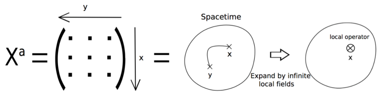
Figure 3: The covariant derivative interpretation of matrix model. $i$ and $j$ of a matrix $(X^{a})_{ij}$ represent two points on a manifold ${\cal{M}}$ (left), and $(X^{a})_{ij}$ operates on a function $f(x)$ as $\sum_{ij}(X^{a})_{ij}f(x_{i})$ (middle). However, by introducing infinite local fields, it can be also represented as a local operator (right).

Among the various solutions, the following one

$$X_{a}=\begin{cases}i\bigtriangledown_{a}=e_{a}^{\mu}(x)\bigtriangledown_{\mu}&\text{for }a=0,1,\cdots,D-1,\\ 0&\text{for }a=D,\cdots,9\end{cases}$$ (22)

is notable because Eq.(21) corresponds to the Einstein equation in this case:

$$\left[\bigtriangledown^{a},\left[\bigtriangledown_{a},\bigtriangledown_{b}\right]\right] =\left[\bigtriangledown^{a},R_{ab}^{cd}\times\hat{{\cal{O}}}_{cd}\right]$$

$$=\left(\bigtriangledown^{a}R_{ab}^{cd}\right)\hat{{\cal{O}}}_{cd}-R_{ab}^{cd}\ \hat{{\cal{O}}}_{cd}\bigtriangledown^{a}=0$$

$$\leftrightarrow \bigtriangledown^{a}R_{ab}^{cd}=0,\ R_{ab}=0$$ (23)

where $\hat{{\cal{O}}}_{cd}$ is the $D$ dimensional Lorentz generator, and we have interpreted $e_{a}^{\mu}(x)$ as the vielbein field. This fact tells us that gravity can be actually embedded in matrix. Furthermore, we can find the diffeomorphism invariance within the original $U(N)$ symmetry:

$$\delta X^{a}=i\left[\Lambda,X^{a}\right],\ \Lambda\in N\times N\ \text{Hermitian matrix}.$$ (24)

The explicit form of $\Lambda$ in the large $N$ limit is given by

$$\Lambda=\lambda(x)+\frac{i}{2}\left\{\lambda^{\mu}(x),\bigtriangledown_{\mu}\right\}+\frac{i^{2}}{2}\left\{\lambda^{\mu\nu}(x),\bigtriangledown_{\mu}\bigtriangledown_{\nu}\right\}+\cdots$$ (25)

as well as $X^{a}$. Here, we have introduced the anti-commutator $\{,\}$ to make each terms hermitian . In particular, the second term

$$\Lambda=\frac{i}{2}\left\{\lambda^{\mu}(x),\bigtriangledown_{\mu}\right\}$$ (27)

represents the diffeomorphism of the fields appearing in Eq.(20). For example, the scalar $S^{a}(x)$ transforms as

$$\delta S^{a}(x)=i\left[\Lambda,S^{a}\right]=\lambda^{\mu}(x)\bigtriangledown_{\mu}S^{a}(x),$$ (28)

and this is actually the diffeomorphism transformation of scalar. Thus, one can see that all the information of a curved manifold ${\cal{M}}$ can be embedded in the matrices $X^{a}$’s. However, the above argument is not mathematically rigorous because $X_{a}=e^{\mu}_{a}(x)\bigtriangledown_{\mu}$ is not in fact included in $End(C^{\infty}({\cal{M}}))$ . To overcome this situation, new formulation of the covariant derivative was proposed in [10] where $X^{a}$’s are interpreted as linear operators acting on smooth functions on the principal bundle $E_{\text{prin}}$ whose base space is ${\cal{M}}$, and fibre is $Spin(D-1,1)$. The result of [10] is mathematically rigorous, so we can actually realize a curved spacetime by matrix. For our present purpose, however, we do not need such a rigorous result, and we take the above naive covariant derivative interpretation in the following discussion.

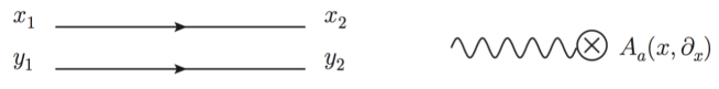
Figure 4: Left: The propagator of the fluctuation $\phi(x,y)$. Right: The background field $A_{a}(x,\partial_{x})$ or $A_{a}(y,\partial_{y})$.

To examine the effective action, we use the background field method:

$$X^{a}(x,y)=\tilde{X}^{a}(x,y)+\phi^{a}(x,y),$$ (30)

where $\tilde{X}^{a}(x,y)$ is the background field, and $\phi^{a}(x,y)$ represents the fluctuation which should be integrated out. The bosonic part of the action Eq.(18) now becomes

$$S_{IIB}\bigg{|}_{boson}=\frac{1}{4g^{2}}\text{Tr}\bigg{(}[\tilde{X}^{a},\tilde{X}^{b}][\tilde{X}_{a},\tilde{X}_{b}] +4[\tilde{X}^{a},\tilde{X}^{b}][\tilde{X}_{a},\phi_{b}]+2[\tilde{X}^{a},\phi^{b}][\tilde{X}_{a},\phi_{b}]+2[\tilde{X}^{a},\tilde{X}^{b}][\phi_{a},\phi_{b}]$$

$$+2[\tilde{X}^{a},\phi^{b}][\phi_{a},\tilde{X}_{b}]+4[\phi^{a},\tilde{X}^{b}][\phi_{a},\phi_{b}]+[\phi^{a},\phi^{b}][\phi_{a},\phi_{b}]\bigg{)},$$ (31)

where the second term can be always eliminated by the field redefinition of $\phi^{a}$. Although there are three quadratic terms in Eq.(31), it is sufficient to consider the third term in Eq.(31) for our qualitative understanding:

$$S_{\phi^{2}}=\frac{1}{2}\text{Tr}\left([\tilde{X}^{a},\phi][\tilde{X}^{a},\phi]\right),$$ (32)

where we have put $g=1$, and picked up one component of $\phi^{a}$’s for simplicity. The effective theory on the flat spacetime can be obtained by expanding the background field around the flat derivative:

$$\tilde{X}^{a}(x,y)=\delta^{(D)}(x-y)\times\begin{cases}i\partial^{a}+A^{a}(x,\partial_{x})&\text{for }a=0,1,\cdots,D-1\\ A^{a}(x,\partial_{x})&\text{for }a=D,\cdots,9\end{cases},$$ (33)

where $A^{a}(x,\partial_{x})$ is a function of $x$ and its derivative, and contains infinite local fields like Eq.(20) and Eq.(25). In this case, Eq.(32) becomes

$$S_{\phi^{2}}=\frac{1}{2}\int d^{D}x\int d^{D}y \left[\left(\frac{\partial}{\partial x^{\mu}}+\frac{\partial}{\partial y^{\mu}}-i{\cal{A}}_{\mu}(x,\partial_{x};y,\partial_{y})\right)\phi(x,y)\right]^{2}$$

$$+\frac{1}{2}\int d^{D}x\int d^{D}y\left[{\cal{A}}_{a}(x,\partial_{x};y,\partial_{y})\phi(x,y)\right]^{2},$$ (34)

where

$${\cal{A}}_{a}(x,\partial_{x};y,\partial_{y})=A_{a}(x,\partial_{x})-A_{a}(y,\partial_{y}).$$ (35)

From Eq.(34), we can read the propagator of $\phi(x,y)$ as

$$D(x_{1},y_{1};x_{2},y_{2}) =G((x_{1}+y_{1})-(x_{2}+y_{2}))\times\delta^{(D)}((x_{1}-y_{1})-(x_{2}-y_{2})),$$ (36)

where $G(x)$ is the propagator of free massless scalar. We represent this propagator and the three (four) point vertex between $\phi$ and the background $A_{a}(x,\partial_{x})$ or $A_{a}(y,\partial_{y})$ by the double lines and the circled cross mark respectively. See Fig.4 for example. Note that only one external wavy line sticks to the vertex because $\phi(x,y)$ interacts $A_{a}(x,\partial_{x})$ or $A_{a}(y,\partial_{y})$.

We can now calculate the effective action

$$\exp\left(iS_{\text{eff}}[{\cal{A}}]\right)=\int{\cal{D}}\phi\ \exp\left(iS_{\phi^{2}}\right)$$ (37)

based on the loop expansion. This is absolutely the same calculation as the effective potential in QFT . For example, at two-loop level, we must calculate the one-loop closed diagram of $\phi(x,y)$ with arbitrary $n$ insertions of $A_{a}$:

$$\int d^{D}x\int d^{D}y\prod_{i=1}^{n}\Bigg{[}\int d^{D}x_{i}\int d^{D}y_{i}D(x_{i+1},y_{i+1};x_{i},y_{i})$$

$$\hskip 56.9055pt\times\begin{cases}\partial^{\mu}A_{\mu}(x_{i},\partial_{x_{i}}),\ \partial^{\mu}A_{\mu}(y_{i},\partial_{y_{i}})\\ \hskip 42.67912pt\text{or}\\ A_{a}(x_{i},\partial_{x_{i}})^{2},\ A_{a}(y_{i},\partial_{y_{i}})^{2},\ 2A^{a}(x_{i},\partial_{x_{i}})A_{a}(y_{i},\partial_{y_{i}})\end{cases}\Bigg{]}\times D(x_{1},y_{1};x,y)$$ (39)

where $x_{n+1}=x$, $y_{n+1}=y$. See the left figure in Fig.5 for example. For our present purpose, it is sufficient to consider the cubic interaction $\phi\phi\partial^{\mu}A_{\mu}$ because our conclusion does not change even if we consider the quartic interaction $\phi\phi A_{a}^{2}$. In order to obtain the effective action written by local fields, let us expand each $A_{a}(x_{i},\partial_{x_{i}})$’s like Eq.(25):

$$A^{a}(x_{i},\partial_{x_{i}}) =\hat{A}^{a}(x_{i})+\frac{i}{2}\left\{\hat{A}^{a\mu}(x_{i}),\partial_{\mu}^{(i)}\right\}+\frac{i^{2}}{2}\left\{\hat{A}^{a\mu\nu}(x_{i}),\partial_{\mu}^{(i)}\partial_{\nu}^{(i)}\right\}+\cdots$$

$$=\sum_{k=0}^{\infty}\frac{i^{n}}{k!}\{\hat{A}^{a\mu_{1}\cdots\mu_{k}}(x_{i}),\partial_{\mu_{1}}^{(i)}\cdots\partial_{\mu_{k}}^{(i)}\}$$

$$=\sum_{k=0}^{\infty}\frac{i^{n}}{k!}\sum_{m=0}^{\infty}\frac{1}{m!}\hat{A}^{a\mu_{1}\cdots\mu_{k}}_{\nu_{1}\cdots\nu_{m}}(x)\{\tilde{x}_{i}^{\nu_{1}}\cdots\tilde{x}_{i}^{\nu_{m}},\tilde{\partial}_{\mu_{1}}^{(i)}\cdots\tilde{\partial}_{\mu_{k}}^{(i)}\}$$

$$:=\sum_{k=0}^{\infty}\frac{i^{n}}{k!}\sum_{m=0}^{\infty}\frac{1}{m!}\hat{A}^{a\{\mu\}}_{\{\nu\}}(x)\hat{\cal{P}}^{(i)\{\nu\}}_{\{\mu\}}(\tilde{x}_{i},\tilde{\partial}^{(i)}).$$ (40)

where $\tilde{x}_{i}=x_{i}-x$, $\tilde{\partial}^{(i)}_{\mu}$ is the derivative with respect to $\tilde{x}_{i}^{\mu}$, and we have expanded $\hat{A}^{a\mu_{1}\cdots\mu_{k}}(x_{i})$ around $x$ from the second line to the third line. Note that we have also used

$$\frac{\partial}{\partial x_{i}^{\mu}}=\frac{\partial}{\partial\tilde{x}_{i}^{\mu}}.$$ (41)

By substituting Eq.(40) into Eq.(39), we generally obtain

$$\int d^{D}x\left(\hat{A}^{\alpha_{1}\{\mu_{1}\}}_{\{\nu_{1}\}}(x)\cdot\cdots\cdot\hat{A}^{\alpha_{l}\{\mu_{l}\}}_{\{\nu_{l}\}}(x)\right)\int d^{D}y\left(\hat{A}^{\beta_{1}\{\mu_{1}\}}_{\{\nu_{1}\}}(y)\cdot\cdots\cdot\hat{A}^{\beta_{f}\{\mu_{f}\}}_{\{\nu_{f}\}}(y)\right)\times\uwave{\left(\prod_{j=1}^{n}\int d^{D}\tilde{x}_{j}\int d^{D}\tilde{y}_{j}\right)}$$

$$\uwave{\times D(x,y;\tilde{x}_{n},\tilde{y}_{n})\times\begin{cases}\tilde{\partial}^{(n)}_{\alpha}\hat{\cal{P}}^{(n)\{\nu\}}_{\{\mu\}}(\tilde{x}_{n},\tilde{\partial}^{(n)})\\ \quad\quad\text{ or }\\ \tilde{\partial}^{(n)}_{\beta}\hat{\cal{P}}^{(n)\{\nu\}}_{\{\mu\}}(\tilde{y}_{n},\tilde{\partial}^{(n)})\end{cases}\times D(\tilde{x}_{n},\tilde{y}_{n};\tilde{x}_{n-1},\tilde{y}_{n-1})\times\cdots\times\begin{cases}\tilde{\partial}^{(1)}_{\alpha}\hat{\cal{P}}^{(1)\{\nu\}}_{\{\mu\}}(\tilde{x}_{1},\tilde{\partial}^{(1)})\\ \quad\quad\text{ or }\\ \tilde{\partial}^{(1)}_{\beta}\hat{\cal{P}}^{(1)\{\nu\}}_{\{\mu\}}(\tilde{y}_{1},\tilde{\partial}^{(1)})\end{cases}}$$

$$\uwave{\times D(\tilde{x}_{1},\tilde{y}_{1};x,y)},$$ (42)

where the numbers $l$ and $f$ depend on the choice of vertexes, and we have changed the variable of each of the integrations from $x_{i}\ (y_{i})$ to $\tilde{x}_{i}\ (\tilde{y}_{i})$. Note that we have not explicitly written the lower index of $\alpha$ ($\beta$) in $\tilde{\partial}_{\alpha}^{(i)}$ ($\tilde{\partial}_{\beta}^{(i)}$) because there are many possible ways of their contractions. Furthermore, from Eq.(36), we can see that $D(\tilde{x}_{1},\tilde{y}_{1};x,y)$ and $D(x,y;\tilde{x}_{n},\tilde{y}_{n})$ do not depend on $x$ and $y$ . As a result, the underlined part in Eq.(42) is just a coefficient, and we finally obtain the factorized bi-local action:

$$c_{\alpha_{1}\cdots\alpha_{l}\beta_{1}\cdots\beta_{f}\{\mu_{1}\}\cdots\{\mu_{l}\},\{\mu_{1}\}\cdots\{\mu_{f}\}}^{\{\nu_{1}\}\cdots\{\nu_{l}\},\{\nu_{1}\}\cdots\{\nu_{f}\}}\int d^{D}x\left(\hat{A}^{\alpha_{1}\{\mu_{1}\}}_{\{\nu_{1}\}}(x)\cdot\cdots\cdot\hat{A}^{\alpha_{l}\{\mu_{l}\}}_{\{\nu_{l}\}}(x)\right)\int d^{D}y\left(\hat{A}^{\beta_{1}\{\mu_{1}\}}_{\{\nu_{1}\}}(y)\cdot\cdots\cdot\hat{A}^{\beta_{f}\{\mu_{f}\}}_{\{\nu_{f}\}}(y)\right).$$ (43)

The reason why we have obtained the bi-local action originates in the number of loops in a diagram: Because one-loop of $\phi$ corresponds to two-loop of the spacetime integrals, the corresponding effective action becomes bi-local. This feature descends to higher loop diagrams. When we consider $m$-loop diagram with arbitrary number of insertion of $A_{a}$’s, we generally obtain

$$\sum_{i_{1},\cdots,i_{m}}c_{i_{1}\cdots i_{m}}\int d^{D}x_{1}{\cal{O}}_{i_{1}}(x_{1})\times\int d^{D}x_{2}{\cal{O}}_{i_{2}}(x_{2})\times\cdots\times\int d^{D}x_{m}{\cal{O}}_{i_{m}}(x_{m}),$$ (44)

where $i_{k}$’s represent the various indexes. See the right figure of Fig.5 for example. Here we show the typical four-loop closed diagram where the self interaction of $\phi$ comes from the last term in Eq.(34). Thus, the effective action $S_{\text{eff}}[{\cal{A}}]$ in the covariant derivative interpretation of matrix model generally contains many multi-local actions, and the effective couplings become dynamical from the previous argument.

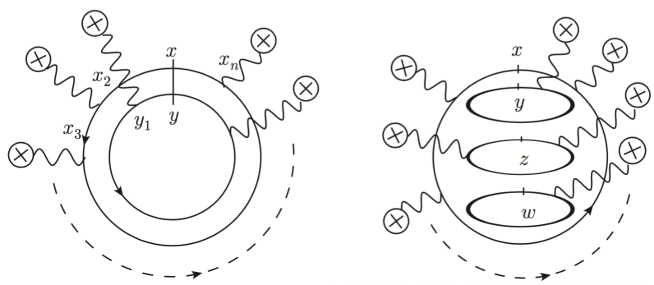
Figure 5: Typical two-loop (left) and four-loop (right) diagrams in the covariant derivative interpretation of matrix model. The number of loops corresponds to the number of the products of the effective actions.

References

- [1] C. D. Froggatt and H. B. Nielsen, “Standard model criticality prediction: Top mass 173 +- 5-GeV and Higgs mass 135 +- 9-GeV,” Phys. Lett. B 368, 96 (1996) doi:10.1016/0370-2693(95)01480-2 [hep-ph/9511371]; C. D. Froggatt, H. B. Nielsen and Y. Takanishi, “Standard model Higgs boson mass from borderline metastability of the vacuum,” Phys. Rev. D 64, 113014 (2001) doi:10.1103/PhysRevD.64.113014 [hep-ph/0104161]; C. D. Froggatt, H. B. Nielsen and L. V. Laperashvili, “Hierarchy-problem and a bound state of 6 t and 6 anti-t,” Int. J. Mod. Phys. A 20 (2005) 1268 doi:10.1142/S0217751X0502416X [hep-ph/0406110]; H. B. Nielsen, “PREdicted the Higgs Mass,” Bled Workshops Phys. 13, no. 2, 94 (2012) [arXiv:1212.5716 [hep-ph]].
- [2] D. Buttazzo, G. Degrassi, P. P. Giardino, G. F. Giudice, F. Sala, A. Salvio and A. Strumia, “Investigating the near-criticality of the Higgs boson,” JHEP 1312, 089 (2013) doi:10.1007/JHEP12(2013)089 [arXiv:1307.3536 [hep-ph]]; S. Iso and Y. Orikasa, “TeV Scale B-L model with a flat Higgs potential at the Planck scale - in view of the hierarchy problem -,” PTEP 2013, 023B08 (2013) doi:10.1093/ptep/pts099 [arXiv:1210.2848 [hep-ph]]; K. Kawana, “Multiple Point Principle of the Standard Model with Scalar Singlet Dark Matter and Right Handed Neutrinos,” PTEP 2015, 023B04 (2015) doi:10.1093/ptep/ptv006 [arXiv:1411.2097 [hep-ph]]; Y. Hamada, H. Kawai, K. y. Oda and S. C. Park, “Higgs inflation from Standard Model criticality,” Phys. Rev. D 91, 053008 (2015) doi:10.1103/PhysRevD.91.053008 [arXiv:1408.4864 [hep-ph]]; K. Kawana, PTEP 2015, 073B04 (2015) doi:10.1093/ptep/ptv093 [arXiv:1501.04482 [hep-ph]]; Y. Hamada, H. Kawai and K. y. Oda, “Eternal Higgs inflation and the cosmological constant problem,” Phys. Rev. D 92, 045009 (2015) doi:10.1103/PhysRevD.92.045009 [arXiv:1501.04455 [hep-ph]]; Y. Hamada and K. Kawana, “Vanishing Higgs Potential in Minimal Dark Matter Models,” Phys. Lett. B 751, 164 (2015) doi:10.1016/j.physletb.2015.10.006 [arXiv:1506.06553 [hep-ph]]. N. Haba and Y. Yamaguchi, “Vacuum stability in the extended model with vanishing scalar potential at the Planck scale,” PTEP 2015, no. 9, 093B05 (2015) doi:10.1093/ptep/ptv121 [arXiv:1504.05669 [hep-ph]]; N. Haba, H. Ishida, R. Takahashi and Y. Yamaguchi, “Gauge coupling unification in a classically scale invariant model,” JHEP 1602, 058 (2016) doi:10.1007/JHEP02(2016)058 [arXiv:1511.02107 [hep-ph]]; N. Haba, H. Ishida, N. Kitazawa and Y. Yamaguchi, “A new dynamics of electroweak symmetry breaking with classically scale invariance,” Phys. Lett. B 755, 439 (2016) doi:10.1016/j.physletb.2016.02.052 [arXiv:1512.05061 [hep-ph]]; N. Haba, H. Ishida, N. Okada and Y. Yamaguchi, “Multiple-point principle with a scalar singlet extension of the Standard Model,” arXiv:1608.00087 [hep-ph].
- [3] Y. Hamada, H. Kawai and K. Kawana, “Natural solution to the naturalness problem: The universe does fine-tuning,” PTEP 2015, no. 12, 123B03 (2015) doi:10.1093/ptep/ptv168 [arXiv:1509.05955 [hep-th]].
- [4] S. R. Coleman, “Why There Is Nothing Rather Than Something: A Theory of the Cosmological Constant,” Nucl. Phys. B 310, 643 (1988). doi:10.1016/0550-3213(88)90097-1.
- [5] Y. Asano, H. Kawai and A. Tsuchiya, “Factorization of the Effective Action in the IIB Matrix Model,” Int. J. Mod. Phys. A 27, 1250089 (2012) doi:10.1142/S0217751X12500893 [arXiv:1205.1468 [hep-th]].
- [6] M. Aaboud et al. [ATLAS Collaboration], “Measurement of the top quark mass in the dilepton channel from TeV ATLAS data,” arXiv:1606.02179 [hep-ex].
- [7] V. Khachatryan et al. [CMS Collaboration], “Measurement of the top quark mass using proton-proton data at = 7 and 8 TeV,” Phys. Rev. D 93, no. 7, 072004 (2016) doi:10.1103/PhysRevD.93.072004 [arXiv:1509.04044 [hep-ex]].
- [8] H. Kawai and T. Okada, “Solving the Naturalness Problem by Baby Universes in the Lorentzian Multiverse,” Prog. Theor. Phys. 127, 689 (2012) doi:10.1143/PTP.127.689 [arXiv:1110.2303 [hep-th]]; Y. Hamada, H. Kawai and K. Kawana, “Evidence of the Big Fix,” Int. J. Mod. Phys. A 29, 1450099 (2014) doi:10.1142/S0217751X14500997 [arXiv:1405.1310 [hep-ph]]; Y. Hamada, H. Kawai and K. Kawana, “Weak Scale From the Maximum Entropy Principle,” PTEP 2015, 033B06 (2015) doi:10.1093/ptep/ptv011 [arXiv:1409.6508 [hep-ph]]; K. Kawana, “Classical conformality in the Standard Model from Coleman’s theory,” arXiv:1605.00436 [hep-ph].
- [9] N. Ishibashi, H. Kawai, Y. Kitazawa and A. Tsuchiya, “A Large N reduced model as superstring,” Nucl. Phys. B 498, 467 (1997) doi:10.1016/S0550-3213(97)00290-3 [hep-th/9612115]; H. Aoki, N. Ishibashi, S. Iso, H. Kawai, Y. Kitazawa and T. Tada, “Noncommutative Yang-Mills in IIB matrix model,” Nucl. Phys. B 565, 176 (2000) doi:10.1016/S0550-3213(99)00633-1 [hep-th/9908141]; H. Steinacker, “Emergent Geometry and Gravity from Matrix Models: an Introduction,” Class. Quant. Grav. 27, 133001 (2010) doi:10.1088/0264-9381/27/13/133001 [arXiv:1003.4134 [hep-th]].
- [10] M. Hanada, H. Kawai and Y. Kimura, “Describing curved spaces by matrices,” Prog. Theor. Phys. 114, 1295 (2006) doi:10.1143/PTP.114.1295 [hep-th/0508211]; H. Kawai, “Curved space-times in matrix models,” Prog. Theor. Phys. Suppl. 171, 99 (2007). doi:10.1143/PTPS.171.99.