Polaritonic linear dynamic in Keldysh formalism

Abstract

We study the dynamic of polaritons in the Keldysh functional formalism. Dissipation is considered through the coupling of the exciton and photon fields to two independent photonic and excitonic baths. As such, this theory allows to describe more intricate decay mechanisms that depend dynamically on the state of the system, such as a direct upper-polariton lifetime, that is motivated from experiments. We show that the dynamical equations in the Keldysh framework otherwise follow the same Josephson–like equations of motions than the standard master equation approach, that is however limited to simple decay channels. We also discuss the stability of the dynamic and reconsider the criterion of strong coupling in the presence of upper polariton decay.

I Introduction

Many-body phenomena in the strong coupling regime of light–matter interactions, in particular Bose-Einstein condensation, have attracted considerable attention in recent yearsdeng10a ; kavokin_book11a . The photon, one of the intrinsic components of the polariton, has an inevitable interaction with the environment, which leads to its decay and often affects the dynamic in a non-negligible way. A well–studied example of non–equilibrium quantum transition takes place in microcavity imamoglu96a . A semiconductor microcavity with embedded low dimensional structures provides a unique laboratory to study a variety of quantum phases. This advantage finds its existence due to a composite boson: the exciton-polariton hopfield58a ; weisbuch92a , a quantum superposition of light and matter with not-only fermionic but also a photonic component. The polaritonic side of the light–matter coupling has stimulated research in both fundamental and applied fields. With regard to the applicability, polaritons promise devices with remarkable upgrades as compared to their semiconductor counterparts, from which polariton lasers imamoglu96a ; christopoulos07a ; daskalakis13a ; azzini11a and polariton transistors amo10a ; ballarini13a ; anton14a ; gao15a are the most obvious examples. Concerning fundamental aspects, polaritons cover immense areas in physics, including Bose-Einstein Condensation (BEC) kasprzak06a ; deng07a ; balili07a ; lai07a , superfluidity carusotto04a ; wouters10b , spin Hall effect kavokin05b , superconductivity laussy10a and Josephson–effects effects lagoudakis10a ; abbarchi13a ; voronova15b ; Rahmani16a .

The simplest description for the kinetic of a polariton gas is provided by semiclasical Boltzmann equations snoke10b . This approach has been used widely by many authors tassone99a ; porras02a ; malpuech02a ; doan05a ; hartwell10a ; maragkou10a . Due to the fast photon leakage from the microcavity, polaritons have a short lifetime, which keeps the polaritonic system in nonequilibrium regime. Therefore the system should be pumped to compensate the losses of polaritons. The rate equation for condensation kinetics of polaritons is:

$$\partial_{t}n_{\mathbf{k}}= p_{\mathbf{k}}-\frac{n_{\mathbf{k}}}{\tau_{\mathbf{k}}}+\frac{\partial n_{\mathbf{k}}}{\partial t}|_{lp-lp}+\frac{\partial n_{\mathbf{k}}}{\partial t}|_{lp-ph}\,,$$ (1)

where $p_{\mathbf{k}}$ is the pumping term, and $(\tau_{\mathbf{k}})^{-1}$ describes the particle decay rate. The two next terms in Eq. (1) account for polariton–polariton and polariton–phonon scattering rates, respectively. We refer to Appendix A for detailed calculations of scattering rates. To illustrate the formation of the condensate in polaritonic system, we present a typical result of numerical simulation of the Boltzmann equation in Fig 1(b). Initially, polaritons are introduced incoherently in exciton–like region of the lower polariton dispersion (Fig. 1(a)), and then relax quickly, except near the exciton–photon resonance. In this region, the polariton density of states is reduced and the photonic contribution to the polariton is increased, which results in polariton accumulations in the bottleneck region tassone97a . This effect is shown as the peak in the curve in Fig. 1(b). To make the population degenerate, that is to overcome the bottleneck effect, one needs to take into account the action of both polariton–polariton and polariton–phonon processes, as the only polariton–phonon scattering mechanism arises pilled up population in non–zero state. With both scattering processes, then Bose stimulation effectively amasses polaritons in the ground state.

While it is a simple, though extremely time consuming, simulation, Boltzmann equations exclude the quantum aspect of the dynamic, to wit, it does not consider the effect of coherence. One then needs to upgrade the formalism to include both quantum and non–equilibrium aspects of the dynamic. A powerful and widely used method that allows such an exact treatment is provided by the Keldysh functional integral approach kamenev_book11a ; sieberer16a . This method has been applied to study the driven open system including polaritons in microcavities szymanska06a ; szyma07a ; proukakis13a ; Dunnett16a ; pavlovic13a , glassy and supperradiant phase of ultracold atoms in optical cavity buchholda13 ; Torre13a , photon condensations in dye filled optical cavity leeuwa13 , etc. It also allows to explore the Bose–Hubbard model with time-dependent hopping kennetta11 , and non–equilibrium Bosonic Josephson oscillations trujilloa09 , among others.

In this paper, a quantum field theory for polariton internal degrees of freedoms in dissipative regime using Keldysh functional method is developed. The need for such an approach in describing the polariton relaxation is motivated mainly by the polariton specificity of providing two types of lifetimes dominici14a : one for the bare states (exciton and photon), the other for the dressed states (upper polariton) skolnick00a . In the latter case, excitons and photons are removed in a correlated way from the system. This effect has attracted attention recently in particular as it can lead to interesting applications proper to polaritons colas15a . While this polariton lifetime can be described in a linear regime from standard master equation approaches, more general scenarios involving, e.g., interactions, get out of reach of this description as the nature of the dressed state changes dynamically with the state of the system. A description of the dissipation therefore needs being made at a more fundamental level than through the standard Lindblad phenomenological form.

While photon and exciton are considered as independent quantum field interacting through the Rabi energy, to model the decay, we assume two independent excitonic and photonic baths, which are present in most light–matter coupled systems. In this text, we restrict our analysis to the linear (Rabi) regime (no interaction). The interaction certainly has important effects, such as self–trapping raghavan99a , and the optical parametric oscillator regime Dunnett16a . However, it can be found that even in the non-interacting regime of the dynamic, some aspects of nonlinearity emerge from the exciton-photon coupling rubo03a ; voronova15a ; Rahmani16a . Therefore, we first attack the problem of polariton dynamics in the Keldysh formalism in the simpler case of non-interacting particles, as a basis for more elaborate and involved studies. At such, we derive the mean–field equations of motions in the photon-exciton basis hampa15 ; elistratova16 ; voronova15a . In particular, we show that the polaritonic internal dynamic satisfies the Josephson criterion of coherent flow.

This paper is organised as follows. In Sec. II we present the polaritonic Hamiltonian and how to turn it into a dissipative system. This includes the Hamiltonian for coupling both bare and dressed fields baths. The Keldysh technique is introduced in Sec. III, where the mean-field solutions and fluctuation actions are also presented. In Sec. IV, we represent the internal dynamic on the Paria sphere Rahmani16a (dynamically renormalized Bloch sphere), and discuss on the stability of the solution. Conclusions are presented in Sec. V.

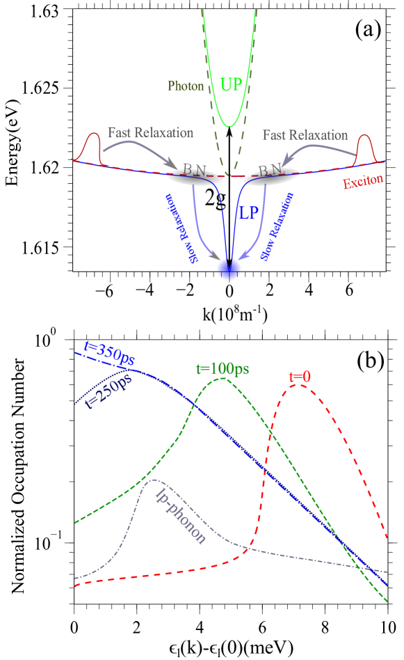
Figure 1: (a) Dispersion of polariton when the detuning at $k=0$ is zero ($\epsilon_{a}(0)=\epsilon_{b}(0)$). Strong coupling between photon (in dash-dark green) and exciton (in dashed red) results the lower polariton (denoted by Lp and in blue) and the upper polariton (denoted by Up and in light green). The energy splitting at $k=0$ is $2g$. In the regime of weak pumping, polaritons are accumulated at the bottleneck region (B.N.). By increasing the pumping strength, the B.N. is relaxed and the condensate forms. The relaxation of polaritons due to interactions with other polariton or phonons is fast in exciton–like region, but is slow in photon–like region. (b) Distribution function of polariton. The initial non–degenerate distribution (red dashed line) evolves to a degenerate distribution (blue dashed–dot line), with both polariton–polariton and polariton–phonon interactions. Considering the phonon–polariton processes only, the distribution remains non–degenerate (gray dashed–dot line). Using parameters for simulation are taken form Ref. doan05a .

II Polariton Hamiltonian

The strong coupling between photon and exciton fields in a semiconductor microcavity results in a quasiparticle with very peculiar properties: the polariton. Denoting the photon and exciton field operators by $a_{\mathbf{k}}$ and $b_{\mathbf{k}}$ respectively, then the Hamiltonian describing the internal coupling between the two fields is given by:

$$H_{c}= H_{0}+H_{Rabi}\,,$$ (2a)

$$H_{0}= \sum_{\mathbf{k}}(\epsilon_{a}(k)a^{\dagger}_{\mathbf{k}}a_{\mathbf{k}}+\epsilon_{b}(k)b^{\dagger}_{\mathbf{k}}b_{\mathbf{k}})\,,$$ (2b)

$$H_{Rabi}= \sum_{\mathbf{k}}g(a^{\dagger}_{\mathbf{k}}b_{\mathbf{k}}+b^{\dagger}_{\mathbf{k}}a_{\mathbf{k}})\,,$$ (2c)

where $\epsilon_{a}$ and $\epsilon_{b}$ are the cavity photon and quantum well exciton dispersion given respectively by:

$$\epsilon_{a}(k)= \frac{\hbar c}{\sqrt{\varepsilon}}\sqrt{k^{2}_{\perp}+k^{2}}\,,$$ (3a)

$$\epsilon_{b}(k)= \epsilon^{ex}(0)+\frac{\hbar^{2}k^{2}}{2m_{ex}}\,,$$ (3b)

with $\epsilon^{ex}(0)=2m_{ex}e^{4}/\varepsilon^{2}\hbar^{2}$ as the 2D exciton binding energy. In Eq. (2c), $g$ shows the strength of coupling between photon and exciton fields and in the regime of strong coupling, it is referred to as the Rabi energy.

Diagonalising the Hamiltonian in Eq. (2a) leads to the new bosonic dressed modes: the lower ($L_{\mathbf{k}}$) and upper ($U_{\mathbf{k}}$) polariton. Then the $H_{c}$ takes the diagonal form:

$$H_{c}=\sum_{\mathbf{k}}\epsilon_{l}L_{\mathbf{k}}^{\dagger}L_{\mathbf{k}}+\epsilon_{u}U_{\mathbf{k}}^{\dagger}U_{\mathbf{k}}\,,$$ (4)

with $\epsilon_{\underset{l}{u}}=\frac{1}{2}(\epsilon_{a}+\epsilon_{b}\pm\sqrt{(\epsilon_{a}-\epsilon_{b})^{2}+(2g)^{2}}$. Note that for zero detuning ($\epsilon_{a}(0)=\epsilon_{b}(0)$), the splitting the two polariton branches is $2g$. The dispersion in zero detuning is shown in Fig. (1).

Such a transformation from bare states (photon and exciton) to dressed states (upper and lower polariton) is done through the operator relation:

$$L_{\mathbf{k}}= A(k)a_{\mathbf{k}}+B(k)b_{\mathbf{k}}\,,$$ (5a)

$$U_{\mathbf{k}}= B(k)a_{\mathbf{k}}-A(k)b_{\mathbf{k}}\,,$$ (5b)

where $A(k)$ and $B(k)$ are the so called Hopfield coefficients hopfield58a , given by ciuti03a ; laussy04b :

$$B(k)=\frac{1}{\sqrt{1+(\frac{g}{\epsilon_{lp}-\epsilon_{c}})^{2}}}\,,$$ (6a)

$$A(k)=-\frac{1}{\sqrt{1+(\frac{\epsilon_{lp}-\epsilon_{c}}{g})^{2}}}\,,$$ (6b)

Due to photon leakage from the microcavity, the polariton has a short lifetime. To consider the dynamic in dissipative regime, one should begin from a microscopic view of the mechanism underling dissipation, namely to model the environmental interaction by coupling the system to a bath. Here the Hamiltonian for the undamped system is given in Eq. (2b), while the baths are modeled as a collection of harmonic oscillators:

$$H_{bath}= \sum_{\mathbf{p}}\omega_{\mathbf{p}}^{ph}r^{\dagger}_{\mathbf{p}}r_{\mathbf{p}}+\sum_{\mathbf{p}}\omega_{\mathbf{p}}^{ex}c^{\dagger}_{\mathbf{p}}c_{\mathbf{p}}\,,$$ (7)

with $\omega_{\mathbf{p}}^{ph(ex)}$ as the dispersion of the photonic (excitonic) bath, and corresponding creation and annihilation operators $r^{\dagger}_{\mathbf{p}}(c^{\dagger}_{\mathbf{p}})$ and $r_{\mathbf{p}}(c_{\mathbf{p}})$, respectively. It is assumed that each bath is in thermal equilibrium and unaffected by the behavior of the system. The bath–system interaction can be described through:

$$H_{Dec}=\sum_{\mathbf{k,p}}[(F_{\mathbf{k}}^{\mathbf{p}}a^{\dagger}+R_{\mathbf{k}}^{\mathbf{p}}b^{\dagger})r+(S_{\mathbf{k}}^{\mathbf{p}}a^{\dagger}+G_{\mathbf{k}}^{\mathbf{p}}b^{\dagger})c]+\mathrm{H.c.}\,,$$ (8)

where $\mathrm{H.c.}$ stands for Hermitian conjugate. Parameters in Eq. (8) are related to the coupling between polaritonic system and baths which are defined as:

$$F_{\mathbf{k}}^{\mathbf{p}} \equiv\Gamma_{\mathbf{k},ph}^{\mathbf{p}}+B\Gamma_{\mathbf{k},u}^{\mathbf{p}}\,,\hskip 14.22636ptR_{\mathbf{k}}^{\mathbf{p}}\equiv-A\Gamma_{\mathbf{k},u}^{\mathbf{p}}\,,$$

$$G_{\mathbf{k}}^{\mathbf{p}} \equiv\Gamma_{\mathbf{k},ex}^{\mathbf{p}}-A\Gamma_{\mathbf{k},u}^{\mathbf{p}}\,,\hskip 14.22636ptS_{\mathbf{k}}^{\mathbf{p}}\equiv B\Gamma_{\mathbf{k},u}^{\mathbf{p}}\,,$$

where $\Gamma_{\mathbf{k},ph(ex)}^{\mathbf{p}}$ shows the coupling strength of the photonic (excitonic) component of the polarion to the photonic (excitonic) bath. The polariton can also decay through its upper branch, which is modeled via direct coupling to the both baths with coupling strength of $\Gamma_{\mathbf{k},u}$. Deriving all the needed Hamiltonian we find for our final Hamiltonian:

$$H= H_{c}+H_{Dec}+H_{bath}\,.$$ (9)

III Functional representation of polaritons

In this section, we present the functional approach to the internal dynamic of polaritons. Any equilibrium many–body theory involves adiabatic switching on of interaction at a distant past ($t=-\infty$), and off at a distant future ($t=\infty$). The state of the system at these two reference times is the ground state of the non–interacting system. Then any correlation function in the interaction representation can be averaged with respect to a known ground state of the non–interacting Hamiltonian.

The postulate of independence of the reference states from the details of switching on and off the interaction breaks in non–equilibrium condition, as the system evolves to an unpredictable state. However, one needs to know the final state. It was Schwinger scwa60 ’s suggestion that the final state to be exactly is the same as that of the initial time. Then the theory can evolve along a two–branch closed time contour with a forward and backward direction.

The central quantity in the functional integral method is the partition function of the system that can be written as a Gaussian integral over the bosonic fields of $\phi,\mathrm{bar}{\phi}$:

$$Z= N~{}\int D[\mathrm{bar}{\phi},\phi]~{}e^{iS[\mathrm{bar}{\phi},\phi]}\,,$$ (10)

where $N$ is the normalization constant and $S$ is the action, which carries the dynamical information. In the Keldysh formalism, the bosonic field $\phi$ is split into two components $\phi^{+}$ and $\phi_{-}$, which reside on the forward and backward part of the time contour. Then the field are rotated to the Keldysh basis defined as:

$$\phi_{\underset{q}{cl}}= \frac{1}{\sqrt{2}}(\phi_{+}\pm\varphi_{-})\,,$$ (11)

where the $+(-)$ sign stands for $cl(q)$. Here $cl(q)$ stands for classical (quantum) component of the field.

Corresponding to the terms in the Hamiltonian (9), the actions take the following components in Keldysh space:

$$S_{0}= \Delta_{\mathbf{k}}^{t}[\Psi_{\mathbf{k}}^{\dagger}(i\partial_{t}-\epsilon_{a})\sigma_{1}^{K}\Psi_{\mathbf{k}}+\Phi_{\mathbf{k}}^{\dagger}(i\partial_{t}-\epsilon_{b})\sigma_{1}^{K}\Phi_{\mathbf{k}}]\,,$$ (12)

$$S_{Rabi}= -\Delta_{\mathbf{k}}^{t}g~{}[\Phi_{\mathbf{k}}^{\dagger}\sigma_{1}^{K}\Psi_{\mathbf{k}}+\Psi_{\mathbf{k}}^{\dagger}\sigma_{1}^{K}\Phi_{\mathbf{k}}]\,,$$ (13)

$$S_{Dec}^{r}= -\Delta_{\mathbf{k,p}}^{t}~{}[(F_{\mathbf{k}}^{\mathbf{p}}\Psi^{\dagger}_{\mathbf{k}}+R_{\mathbf{k}}^{\mathbf{p}}\Phi^{\dagger}_{\mathbf{k}})\sigma^{K}_{1}X_{R,\mathbf{p}}+\mathrm{h.c.}]\,,$$ (14)

$$S_{Dec}^{c}= -\Delta_{\mathbf{k,p}}^{t}~{}[(S_{\mathbf{k}}^{\mathbf{p}}\Psi^{\dagger}_{\mathbf{k}}+G_{\mathbf{k}}^{\mathbf{p}}\Phi^{\dagger}_{\mathbf{k}})\sigma^{K}_{1}X_{C,\mathbf{p}}+\mathrm{h.c.}]\,,$$ (15)

$$S_{bath}= \Delta_{\mathbf{p}}^{t}~{}\sum_{j=R,C}X_{j,\mathbf{p}}^{\dagger}(i\partial_{t}-\omega_{\mathbf{p}}^{j})\sigma_{1}^{K}X_{j,\mathbf{p}}$$

$$= \Delta_{\mathbf{p}}^{t}~{}\sum_{j=R,C}X_{j,\mathbf{p}}^{\dagger}C_{j}^{-1}X_{j,\mathbf{p}}\,,$$ (16)

where we use $\Delta_{\mathbf{k}}^{t}$ as an abbreviation for $\sum_{\mathbf{k}}\int_{-\infty}^{\infty}~{}dt$, and superscript $r$ and $c$ refer to excitonic and photonic baths, respectively. Other notations are summarised in Table 1.

Table 1: Fields and matrices in Keldysh space

Fields in Keldysh space
Photonic	Ecxitonic	Photonic Bath	Excitonic Bath
$\Psi_{\mathbf{k}}$	$\Phi_{\mathbf{k}}$	$X_{c,\mathbf{k}}$	$X_{r,\mathbf{k}}$
$\left(\begin{array}[]{c}\psi_{cl}\\ \psi_{q}\end{array}\right)_{\mathbf{k}}$	$\left(\begin{array}[]{c}\varphi_{cl}\\ \varphi_{q}\end{array}\right)_{\mathbf{k}}$	$\left(\begin{array}[]{c}x_{cl}\\ x_{q}\end{array}\right)_{\mathbf{k}}$	$\left(\begin{array}[]{c}y_{cl}\\ y_{q}\end{array}\right)_{\mathbf{k}}$
Pauli matrices in Keldysh space
$\sigma_{K}^{0}$	$\sigma_{K}^{1}$	$\sigma_{K}^{2}$	$\sigma_{K}^{3}$
$\left(\begin{array}[]{cc}1&0\\ 0&1\end{array}\right)$	$\left(\begin{array}[]{cc}0&1\\ 1&0\end{array}\right)$	$\left(\begin{array}[]{cc}0&-i\\ i&0\end{array}\right)$	$\left(\begin{array}[]{cc}1&0\\ 0&-1\end{array}\right)$

The bath action in Eq. (III) is in the standard form in Keldysh space: it contains a quadratic form of the fields with a matrix which is the inverse of a correlator $C_{j}$ with $j=\left\{r,c\right\}$. One can show that:

$$C_{j}\equiv \left(\begin{array}[]{cc}C^{K}_{i}&C^{R}_{j}\\ C^{A}_{j}&0\end{array}\right)_{t,t^{\prime}}$$ (19)

$$= \left(\begin{array}[]{cc}-if_{j}e^{-i\omega_{p}^{j}(t-t^{\prime})}&-i\Theta(t-t^{\prime})e^{-i\omega_{p}^{j}(t-t^{\prime})}\\ i\Theta(t-t^{\prime})e^{-i\omega_{p}^{j}(t-t^{\prime})}&0\end{array}\right)\,,$$ (22)

where $\Theta(t)$ is the Heaviside step function and $f_{j}$ is the distribution function of the bath.

As the bath coordinates appear in a quadratic form, they can be integrated out to reduce the degree of freedom to photon and exciton fields only. We follow the procedure described in Refs. kamenev_book11a ; szyma07a . Employing the properties of Gaussian integration, the decay bath eliminating leads to two effective actions:

$$S_{Dec}^{r}= \Delta_{\mathbf{k,p}}^{t,t^{\prime}}~{}(F_{\mathbf{k}}^{\mathbf{p}}\Psi^{\dagger}_{\mathbf{k}}+R_{\mathbf{k}}^{\mathbf{p}}\Phi^{\dagger}_{\mathbf{k}})_{t}~{}\mathcal{C}^{-1}_{r}(t-t^{\prime})~{}(F_{\mathbf{k}}^{\mathbf{p}}\Psi_{\mathbf{k}}+R_{\mathbf{k}}^{\mathbf{p}}\Phi_{\mathbf{k}})_{t^{\prime}}\,,$$ (23a)

$$S_{Dec}^{c}= \Delta_{\mathbf{k,p}}^{t,t^{\prime}}~{}(S_{\mathbf{k}}^{\mathbf{p}}\Psi^{\dagger}_{\mathbf{k}}+G_{\mathbf{k}}^{\mathbf{p}}\Phi^{\dagger}_{\mathbf{k}})_{t}~{}\mathcal{C}^{-1}_{c}(t-t^{\prime})~{}(S_{\mathbf{k}}^{\mathbf{p}}\Psi_{\mathbf{k}}+G_{\mathbf{k}}^{\mathbf{p}}\Phi_{\mathbf{k}})_{t^{\prime}}\,,$$ (23b)

where $\mathcal{C}^{-1}_{j}(t-t^{\prime})=-\sigma_{1}^{K}~{}[C_{j}(t-t^{\prime})]~{}\sigma_{1}^{K}$ and $j=\left\{r,c\right\}$. Straightforward matrix multiplication shows that the $\mathcal{C}^{-1}$ correlator has the causality structure, given by:

$$\mathcal{C}^{-1}_{j}(t-t^{\prime})\equiv \left(\begin{array}[]{cc}0&\mathcal{C}^{A}_{j}\\ \mathcal{C}^{R}_{j}&\mathcal{C}^{K}_{j}\end{array}\right)_{t,t^{\prime}}\,.$$ (26)

To proceed further, we make some simplifying assumptions about the baths. Firstly, we assume that all modes of the systems are coupled to their baths with the same strength, i.e, $\Gamma_{j}(p)\equiv\Gamma_{\mathbf{k},j}^{\mathbf{p}}$. Besides, it is assumed that the bath is in the Markovian limit, where the density of state for the baths and the coupling between the system and baths are constant. In the following, we restrict our analysis to these assumptions. More details including non–Markovian cases are presented in Appendix B.

Denoting the decay action as $S_{Dec}=\sum_{i=r,c}S_{bath}^{i}+S_{Dec}^{i}$, one gets the components of the $S_{D}$ as (see Appendix B):

$$S_{Dec}^{1}= \sum_{\mathbf{k}}\int~{}dt\{\gamma_{1}(k)\Psi^{\dagger}_{\mathbf{k}}\sigma_{2}^{K}\Psi_{\mathbf{k}}$$ (27)

$$+2i(\gamma_{1}(k))\int dt^{\prime}\mathrm{bar}{\psi}_{q}(t)(f_{c}+f_{d})_{t-t^{\prime}}\psi_{q}(t^{\prime})\}\,,$$

$$S_{Dec}^{2}= \sum_{\mathbf{k}}\int~{}dt\{\gamma_{2}(k)\Phi^{\dagger}_{\mathbf{k}}\sigma_{2}^{K}\Phi_{\mathbf{k}}$$ (28)

$$+2i(\gamma_{2}(k))\int dt^{\prime}\mathrm{bar}{\varphi}_{q}(t)(f_{c}+f_{d})_{t-t^{\prime}}\varphi_{q}(t^{\prime})\}\,,$$

$$S_{Dec}^{3}= \sum_{\mathbf{k}}\int~{}dt\{\gamma_{3}(k)\Psi^{\dagger}_{\mathbf{k}}\sigma_{2}^{K}\Phi_{\mathbf{k}}$$ (29)

$$+2i(\gamma_{3}(k))\int dt^{\prime}\mathrm{bar}{\psi}_{q}(t)(f_{c}+f_{d})_{t-t^{\prime}}\varphi_{q}(t^{\prime})\}\,,$$

$$S_{Dec}^{4}= \sum_{\mathbf{k}}\int~{}dt\{\gamma_{3}(k)\Phi^{\dagger}_{\mathbf{k}}\sigma_{2}^{K}\Psi_{\mathbf{k}}$$ (30)

$$+2i(\gamma_{3}(k))\int dt^{\prime}\mathrm{bar}{\varphi}_{q}(t)(f_{c}+f_{d})_{t-t^{\prime}}\psi_{q}(t^{\prime})\}\,,$$

where we define $\gamma_{1}=B^{2}\gamma_{u}^{2}+(\gamma_{a}+B\gamma_{u})^{2}$, $\gamma_{2}=A^{2}\gamma_{u}^{2}+(\gamma_{b}-A\gamma_{u})^{2}$, $\gamma_{3}=\gamma_{u}(B(\gamma_{b}-A\gamma_{u})-A(\gamma_{a}+B\gamma_{u}))$, and $\sigma^{K}_{2}$ is given in Table 1. One notes that with decay for the upper polariton, the decay action has the weightings of excitonic and photonic Hopfield coefficients; moreover, even without bare field couplings $\gamma_{a}$ and $\gamma_{b}$, the decay in the upper branch is enough to remove the photon and exciton fields both independently and in a correlated way.

III.1 Mean field solutions

Having integrated out the bath degree of freedom, the action appears in its final form as: $S=S_{0}+S_{R}+S_{Dec}$. We can then obtain the equations of motions from the saddle point condition on the action:

$$\frac{\partial S}{\partial\mathrm{bar}{\psi}_{i=q,cl}}=0\,,\hskip 14.22636pt\frac{\partial S}{\partial\mathrm{bar}{\varphi}_{i=q,cl}}=0\,.$$ (31)

which yields:

$$\frac{\partial S}{\partial\mathrm{bar}{\psi}_{q}}= (i\partial_{t}-\epsilon_{a}+i\gamma_{1})\psi_{cl}-(g-i\gamma_{3})\varphi_{cl}$$

$$+2i\gamma_{1}\int~{}dt^{\prime}(f_{c}+f_{d})(t-t^{\prime})\psi_{q}(t^{\prime})$$

$$+2i\gamma_{3}\int~{}dt^{\prime}(f_{c}+f_{d})(t-t^{\prime})\varphi_{q}(t^{\prime})\,,$$ (32a)

$$\frac{\partial S}{\partial\mathrm{bar}{\varphi}_{q}}= (i\partial_{t}-\epsilon_{b}+i\gamma_{2})\varphi_{cl}-(g-i\gamma_{3})\psi_{cl}$$

$$+2i\gamma_{2}\int~{}dt^{\prime}(f_{c}+f_{d})(t-t^{\prime})\varphi_{q}(t^{\prime})$$

$$+2i\gamma_{3}\int~{}dt^{\prime}(f_{c}+f_{d})(t-t^{\prime})\psi_{q}(t^{\prime})\,,$$ (32b)

$$\frac{\partial S}{\partial\mathrm{bar}{\psi}_{cl}}= (i\partial_{t}-\epsilon_{a}-i\gamma_{1})\psi_{q}-(g+i\gamma_{3})\varphi_{q}\,,$$ (32c)

$$\frac{\partial S}{\partial\mathrm{bar}{\varphi}_{cl}}= (i\partial_{t}-\epsilon_{b}-i\gamma_{2})\varphi_{q}-(g+i\gamma_{3})\psi_{q}\,.$$ (32d)

One notices that Eqs.(32c-32d) are satisfied by $\varphi_{q}=\mathrm{bar}{\varphi}_{q}=0$ and $\psi_{q}=\mathrm{bar}{\psi}_{q}=0$, irrespective of what the classical components, $\varphi_{0}\equiv\varphi_{cl}$ and $\varphi_{0}\equiv\varphi_{cl}$, are. Then, under these conditions, Eqs. (32-32) lead to:

$$\partial_{t}\psi_{0}= (-i\epsilon_{a}-\gamma_{1})\psi_{0}+(-ig-\gamma_{3})\varphi_{0}\,,$$ (33)

$$\partial_{t}\varphi_{0}= (-i\epsilon_{b}-\gamma_{2})\varphi_{0}+(-ig-\gamma_{3})\psi_{0}\,.$$ (34)

These equations provide an extreme limit for the action $S$ and describe the system of two coupled-equations of motions in the mean field analysis.

III.2 Fluctuations of the action

By separating the fluctuations from the mean field:

$$\psi=\psi_{0}+\delta\psi_{cl}\,,\hskip 14.22636pt\psi_{q}=\delta\psi_{q}\,,$$ (35)

$$\varphi=\varphi_{0}+\delta\varphi_{cl}\,,\hskip 14.22636pt\varphi_{q}=\delta\varphi_{q}\,,$$ (36)

for the actions defined in Eqs. (12)–(13) and (27)–(30), then employing the Fourier transform, the fluctuating action takes the form:

$$\Delta S=\int~{}d\omega\sum_{\mathbf{k}}\Delta\mathcal{T}_{\mathbf{k}}^{\dagger}\left(\begin{array}[]{c|c}0&[\mathcal{F}^{-1}]^{A}\\ \hline\cr[\mathcal{F}^{-1}]^{R}&[\mathcal{F}^{-1}]^{K}\end{array}\right)\Delta\mathcal{T}_{\mathbf{k}}\,,$$ (39)

where the superscripts $A$, $R$, and $K$ stand for the advanced, retarded and Keldysh components of the inverse Green function, respectively. The fluctuation vector has the form of:

$$\Delta\mathcal{T}_{\mathbf{k}}^{\dagger}\equiv(CL,Q)^{T}$$ (40)

with

$$CL\equiv\left(\begin{array}[]{c}\delta\mathrm{bar}{\psi}_{cl}(\omega)\\ \delta\psi_{cl}(-\omega)\\ \delta\mathrm{bar}{\varphi}_{cl}(\omega)\\ \delta\varphi_{cl}(-\omega)\end{array}\right)_{\mathbf{k}}\quad\text{and}\quad Q\equiv\left(\begin{array}[]{c}\delta\mathrm{bar}{\psi}_{q}(\omega)\\ \delta\psi_{q}(-\omega)\\ \delta\mathrm{bar}{\varphi}_{q}(\omega)\\ \delta\varphi_{q}(-\omega)\end{array}\right)_{\mathbf{k}}\,.$$ (49)

Further, the off–diagonal matrix elements in Eq. (39) have the following relations kamenev_book11a :

$$[\mathcal{F}^{-1}]^{R(A)}~{}\mathcal{F}^{R(A)}=1\,,$$ (50)

$$\mathcal{F}^{A}=(\mathcal{F}^{R})^{\dagger}\,,$$ (51)

while for the diagonal element one finds:

$$\mathcal{F}^{K}=\mathcal{F}^{R}F-F\mathcal{F}^{A}$$ (52)

where  $F$ is referred to as the distribution function of the system kamenev_book11a . Having found the Green functions of the dynamic, one can decide about the stability of the solution by studying the retarded Green function, namely by solving $\det([\mathcal{F}^{-1}]^{R}(\omega_{r}))=0$, where $\omega_{r}$ is the pole of the retarded Green function. If $\mathrm{Im}[\omega_{r}]<0$, then the proposed solution is stable.

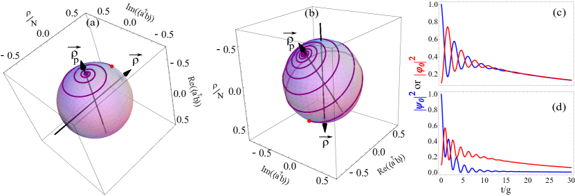
Figure 2: (a) The internal dynamic of polariton in a photon–like point on the Paria sphere, when detuning between exciton and photon fields is zero. The $\rho_{p}$ direction shows the orientation of the upper–lower polariton states, while the $\rho$ shows the direction of exciton–photon states. The red point shows the initial point. (b) The same as (a) but for an exciton–like point. (c) and (d) shows the population dynamic in photon and exciton like point respectively. Using parameters are: $\gamma_{a}=0.2g$, $\gamma_{b}=0.02g$, $\gamma_{u}=0.3g$.

IV Discussion

To analyse the equations of motions, we start from Eqs. (33) and (34), and restrict calculations to two points in reciprocal space: the space center ($k=0$), that is a photon–like point, and an exciton–like point at $k\sim\sqrt{2m_{ex}\epsilon_{ex}^{0}}$. In the absence of exciton and photon detuning at $k=0$, the coupling fields are at resonance, and the exciton and photon have the same weight of $1/2$ in the polariton. However, bare states at $k\neq 0$ are positively detuned, which provides an intrinsic detuning in the internal dynamic of polaritons.

Introducing $\rho_{\mathbf{k}}\equiv\frac{1}{2}(|\psi_{0}|^{2}-|\varphi_{0}|^{2})$ as the population imbalance and $N_{\mathbf{k}}\equiv(|\psi_{0}|^{2}+|\varphi_{0}|^{2})$ as the total field population in state $\mathbf{k}$, one can show that the Eqs. (33) and (34) are in the form of Josephson equations, that is:

$$\partial_{t}(\rho/N)_{\mathbf{k}}= -\sqrt{1-4(\rho/N)_{\mathbf{k}}^{2}}(g\sin(\sigma_{\mathbf{k}})-\gamma_{3}\cos(\sigma_{\mathbf{k}})(\rho/N)_{\mathbf{k}})$$

$$-(\gamma_{1}+\gamma_{2})(1-4(\rho/N)_{\mathbf{k}}^{2})\,,$$ (53a)

$$\partial_{t}\sigma_{\mathbf{k}}= -\delta_{\mathbf{k}}$$

$$+\frac{1}{\sqrt{1-4(\rho/N)_{\mathbf{k}}^{2}}}(4g\cos(\sigma_{\mathbf{k}})(\rho/N)_{\mathbf{k}}+\gamma_{3}\sin(\sigma_{\mathbf{k}}))\,,$$ (53b)

where $\delta_{\mathbf{k}}=\epsilon_{a}-\epsilon_{b}$ stands for detuning between the states, and $\sigma_{\mathbf{k}}=\arg[\psi_{0}^{\ast}\varphi_{0}]$ is the relative phase between bare states. With such a representation of the dynamic, each polaritonic state in $\mathbf{k}$ has an intrinsic internal Josephson–like dynamic, when the relative phase drives the population difference. Recently, the same equations of motions were reported by one of the authors, but for an effective two-level system and in a different formalism Rahmani16a ; Rahmani16wolfram . One notices that the phase difference between the two coupled fields, with a definite phase in each field, is crucial to drive the internal dynamic. This is the case when two or more condensates are coupled, through for example Josephson junctions. However, here we do not take any assumption about the condensate phase, and this is left to the initial condition to define a clear phase for each field; then as long as the polaritonic system is initially prepared by a source of specific phase, the internal dynamic follows the Josephson dynamic, and the coherence oscillates between the fields.

An example of the dynamic is shown in Fig. (2). Here we adopt the Paria sphere Rahmani16wolfram to observe the dynamic in a three dimensional representation. Two directions are indicated on the sphere: the $\vec{\rho}$ direction, that shows the direction for exciton–photon states, and $\vec{\rho}_{p}$, which shows the orientation of lower–upper polariton states. Starting from an initial point (the red point in Fig. (1)), the dynamic goes toward a fixed point (when the sphere is kept normalized). In the zero detuning case, (Fig (2–a)), the laboratory basis is orthogonal to the dressed state basis, with $\vec{\rho}\perp\vec{\rho}_{p}$, and the relative phase remains in an oscillatory mode. Going toward an exciton–like point in Fig (2–b), the two directions are not orthogonal, that shows the final state has a more exciton weight. At the same time, one can see a switching from the running mode to the oscillatory mode in relative phase, which is mediated by decay. We also show the dynamic of bare state populations in photon–like (Fig. (2–c)) and exciton–like(Fig. (2–d)) points of the indirect space. We set the initial conditions to have more population in the photon field. At zero detuning, both fields are oscillating in the same trend, as the decay affects the dynamic equivalently; however, by increasing the detuning, decay affects the field (in this example the photon field) that has the more population. In other words, by increasing the detuning, bare states become decoupled and each field loses its coupling to other fields while the coupling to the bath is yet active.

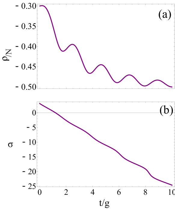
Figure 3: (a) damped oscillations in population imbalance mediated by decay in the upper polariton. Corresponding relative phase is shown in (b). Parameters used are: $\delta=3g,~{}\gamma_{a}=\gamma_{b}=.2g,~{}\gamma_{u}=.6g,~{}\rho(0)=-0.3N,~{}\sigma(0)=\pi$.

The equations of motions in their Josephson representation bring a new variant for the dynamics of polariton. Careful inspection in Eqs. (53) shows that the relative phase is driving the population in two ways: one is the well–studied Josephson dynamic with the term proportional to $g\sin(\sigma_{\mathbf{k}})$ in the equations form Ref. raghavan99a . The other comes from the term proportional to $\gamma_{3}\cos(\sigma_{\mathbf{k}})(\rho/N)_{\mathbf{k}}$, which existence is related to the upper polariton decay, and is specific to this phenomenon. Such a peculiar aspect of the dynamic holds even for the case of disconnected fields which are correlatively coupled to a bath. A particular example of the internal dynamic mediated only by polariton decay is shown in Fig. (3). As the relative phase is in the running mode, the population imbalance exhibit damped oscillations toward a fixed point.

In any dynamical system, the stability of the solution in the steady state is the most important property. In normalized coordinates, the fixed points of the dynamic have a finite values, even in the dissipative regime Rahmani16a . For a given fixed point, the stability condition is determined through the inverse retarded Green function in Eq. (39), which reads:

$$[\mathcal{F}^{-1}]^{R}(\omega,\mathbf{k})=\frac{1}{2}\left(\begin{array}[]{cccc}\omega-\epsilon_{a}+i\gamma_{1}&0&-g+i\gamma_{3}&0\\ 0&-\omega-\epsilon_{a}-i\gamma_{1}&0&-g-i\gamma_{3}\\ -g+i\gamma_{3}&0&\omega-\epsilon_{b}+i\gamma_{2}&0\\ 0&-g-i\gamma_{3}&0&-\omega-\epsilon_{b}-i\gamma_{2}\end{array}\right)\,.$$ (58)

One notices how coupling between photon and exciton fields are reflected as the coupling between quantum and classical parts of the fields in Keldysh space, which makes the retarded matrix non–diagonal. More interestingly is the appearance of the term $\gamma_{3}$, which has the same weight in the dynamic as the coupling-constant $g$. This is the direct consequence of the decay in the upper polariton branch, as it removes bare fields in a correlated fashion.

Solving $[\det(\mathcal{F}^{-1}]^{R}(\omega_{r})=0$, one finds the energies of the dressed states in the dissipative regime as:

$$\omega_{r}^{\pm}= \frac{1}{2}[\epsilon_{a}+\epsilon_{b}-i(\gamma_{1}+\gamma_{2})$$

$$\pm\sqrt{(\delta_{\mathbf{k}}-2ig-\gamma_{+})(\delta_{\mathbf{k}}+2ig-\gamma_{-})}]\,,$$ (59)

where $\delta_{\mathbf{k}}=\epsilon_{a}-\epsilon_{b}$ is the detuning, and $\gamma_{\pm}=\pm 2\gamma_{3}+i(\gamma_{1}-\gamma_{2})$. The version with no dissipation has the familiar form elistratova16 :

$$\omega_{r}^{\pm}= \frac{1}{2}(\epsilon_{a}+\epsilon_{b}\pm\sqrt{\delta_{\mathbf{k}}+4g^{2}})\,,$$ (60)

that is the result from a pure Hamiltonian picture (see the notes after Eq. 4). For zero detuning, one gets:

$$\omega_{r}^{\pm}= \frac{1}{2}[\epsilon_{a}+\epsilon_{b}-i(\gamma_{1}+\gamma_{2})$$

$$\pm\sqrt{(-2ig-\gamma_{+})(+2ig-\gamma_{-})}]\,.$$ (61)

For $\gamma_{3}=0$, the term under the square root can go from real to imaginary, namely, it happens when $g<(\gamma_{1}-\gamma_{2})/2$, which is considered as the criterion for strong to weak coupling transition laussy08a ; kavokin_book11a . However, for $\gamma_{3}\neq 0$, we see clearly that the term under the square root remains imaginary, which breaks the criterion of strong-to-weak coupling transition at zero detuning. The imaginary parts of $\omega^{\pm}_{r}$ determine the stability of the solutions. Straightforward calculations lead to:

$$\mathrm{Im}[\omega_{r}^{\pm}]=-(\gamma_{1}+\gamma_{2})-\sqrt{\frac{-\mathbb{IM}+\sqrt{\mathbb{IM}^{2}+\mathbb{RE}^{2}}}{2}}\,,$$ (62)

where $\mathbb{IM}=-2\delta_{\mathbf{k}}(\gamma_{1}-\gamma_{2})-8g\gamma_{3}$ and $\mathbb{RE}=\delta_{\mathbf{k}}^{2}-(\gamma_{1}-\gamma_{2})^{2}+4(g^{2}-\gamma_{3}^{2})$. Clearly, it can be seen that the imaginary part of the $\omega_{r}^{\pm}$, for given parameters of the system, always remains negative, which results in stable solutions. One direct consequence of such stability is the resistance of the system against phase transitions, which is the case in presence of interactions and pumping. Clearly, the combination of decay and interaction makes the dynamics richer and their full effects will be discussed in future works.

V Conclusion

In conclusion, we study the internal dynamic of polariton in the Keldysh functional approach, when fields are removed from both bare and dressed states. In the linear Rabi regime, the coupled equations of motions are local in reciprocal space, and the intrinsic detuning between bare states works as an intrinsic potential affecting the dynamic. It is shown also that the equations of motions are in the form of Josephson equations, but that the upper-polariton lifetime (correlated decay of the dressed state) brings a peculiar feature in the dynamics, namely, it mediates an internal dynamic between the bare states. This would happen even if the bare states would be decoupled (although then the origin for their correlated decay would be less clear on physical grounds). Considering the retarded Green functions, we show that the dynamic in the Rabi regime is stable, and the criterion of strong coupling is fragile in presence of an upper polariton decay.

Appendix A

Here we describe two important scattering mechanisms in the polariton kinetic. Main equations for numerical calculation are presented.

A.1 polariton–polariton scattering

Suppose the occupation number of state $\mathbf{k}$ is given by $n_{\mathbf{k}}$, then the time variation of the occupation number due to polariton–polariton interaction reads:

$$\frac{\partial n_{\mathbf{k}}}{\partial t}|_{lp-lp}= -n_{\mathbf{k}}\sum_{\mathbf{k^{\prime}},\mathbf{q}}W^{lp-lp}_{\mathbf{k}^{\prime}\mathbf{k}}(n_{\mathbf{k}^{\prime}}+1)(n_{\mathbf{q}}+1)n_{\mathbf{k^{\prime}}+\mathbf{q}-\mathbf{k}}$$

$$+(n_{\mathbf{k}}+1)\sum_{\mathbf{k}^{\prime},\mathbf{q}}n_{\mathbf{k}^{\prime}}n_{\mathbf{q}}(n_{\mathbf{k}^{\prime}+\mathbf{q-k}}+1)W^{lp-lp}_{\mathbf{k}\mathbf{k}^{\prime}}\,,$$ (63)

where $W^{lp-lp}_{\mathbf{k}\mathbf{k}^{\prime}}$ is the polariton–polariton scattering rate for transition of polariton form state $\mathbf{k}$ to $\mathbf{k^{\prime}}$. Using the Fermi’s golden rule, the scattering rate reads:

$$W_{\mathbf{k,k^{\prime}}}^{lp-lp}=\frac{2\pi}{\hbar}B_{eff}|M(|\mathbf{k-k^{\prime}}|)|^{2}\delta(E_{k}+E_{k_{s}}-E_{q}-E_{k^{\prime}})\,,$$ (64)

with $B_{eff}=B(k)^{2}B(k^{\prime})^{2}B(q)^{2}B(k_{s})^{2}$ as the effective excitonic weight, and $\mathbf{k}_{s}=\mathbf{k^{\prime}+q-k}$. The exciton–exciton matrix element, $M$, has been studied by Ciuti et al. ciuti98a and recently by Sun et al. arXiv_sun . Here we use the estimation provided by Tassone and Yamamoto tassone99a as $M\approx 6a_{B}^{2}\epsilon^{ex}/A_{s}$, where $a_{B}$ is the two dimensional Bohr radios of the exciton, and $A_{s}$ is the area of the sample. Replacing the sum by integral (thermodynamic limit) and employing the properties of delta function one gets:

$$\frac{\partial n_{\mathbf{k}}}{\partial t}|_{lp-lp}= \frac{A_{s}^{2}}{8\pi^{3}\hbar}\int k^{\prime}dk^{\prime}qdqd\theta^{\prime}B_{eff}M^{2}(\frac{\partial\epsilon_{l}}{\partial k_{s}^{2}})^{-1}$$

$$\times[\frac{n_{k}n_{k_{s}}(1+n_{q})(1+n_{k^{\prime}})}{((c_{min}-\cos(\theta^{\prime}))(\cos(\theta^{\prime})-c_{max}))^{1/2}}$$

$$+\frac{n_{k^{\prime}}n_{q}(1+n_{k_{s}})(1+n_{k})}{((c_{min}-\cos(\theta^{\prime}))(\cos(\theta^{\prime})-c_{max}))^{1/2}}]\,,$$ (65)

where $c_{min}(c_{max})$ is the lower (upper) limit of integrations over $\theta^{\prime}$, and is of the form:

$$c_{min(max)}=\frac{k^{2}+k^{\prime 2}-(k_{s}\mp q)^{2}}{2kk^{\prime}}\,.$$ (66)

A.2 polariton–phonon scattering

Polariton can scatter from one state to other states through emission or absorption of phonons. The time variation of the occupation number caused by polariton–phonon scattering reads:

$$\frac{\partial n_{\mathbf{k}}}{\partial t}|_{lp-ph}=I_{in}^{abs}+I_{in}^{em}+I_{out}^{abs}+I_{out}^{em}\,,$$ (67)

where the portion of emission and absorption of phonon in polariton scattering is shown by superscript $em$ and $abs$ respectively. Here we describe, for example, $I_{in}^{em}$ in details. This term describes polariton scattering rate form $\mathbf{k^{\prime}}$ to $\mathbf{k}$ while a phonon is absorbed. Other terms in Eq. (67) can be drived straightforwardly. Utilizing the Fermi’s golden rule, one finds

$$I_{in}^{em}=(n_{\mathbf{k}}+1)\frac{2\pi}{\hbar}\sum_{\mathbf{k}^{\prime},q_{z}}W^{2}n_{\mathbf{k^{\prime}}}n_{\mathbf{Q}}~{}\delta(E_{k^{\prime}}-E_{k}-E_{Q})\,,$$ (68)

where we call $\mathbf{Q}=(\mathbf{q=k-k^{\prime}},q_{z})$ the phonon wavevector, and $W$ stands for transition probability. We restrict our analysis to longitudinal–acoustic phonon, for which the polariton–phonon interaction is provided by the deformation–potential coupling with electron and hole $D_{e}$ and $D_{h}$, correspondingly. Taking $\mathbf{r}_{i=e,h}=(\boldsymbol{\rho}_{i},z_{i})$ and $\boldsymbol{\rho}=\boldsymbol{\rho}_{e}-\boldsymbol{\rho}_{h}$ , the exciton wavefunction in state $\mathbf{k}$ is given by $\langle\mathbf{r}_{e},\mathbf{r}_{h}|\mathbf{k}\rangle=\frac{1}{\sqrt{A_{s}}}\exp(i\mathbf{k}\cdot\mathbf{R})f(\mathbf{\rho})U_{e}(z_{e})U_{h}(z_{h})$. Then the transition probability reads

$$W=B(k)B(k^{\prime})\sqrt{\frac{\hbar Q}{2\rho_{d}uV}}\mathbb{D}(|\mathbf{k-k^{\prime}}|)\mathbb{A}(q_{z})\delta_{\mathbf{q,k-k^{\prime}}}\,,$$ (69)

where $\mathbb{A}=\int dz_{e}e^{iq_{z}z_{e}}U^{2}_{e}(z_{e})$ and $\mathbb{D}=D_{e}G(\beta_{h}q)+D_{h}G(-\beta_{e}q)$. The form factor $G$ is defined $G(x)=\int f^{2}e^{i\mathbf{x}\cdot\boldsymbol{\rho}}d\boldsymbol{\rho}$. Replacing the sum with integral in Eq. (68) we finally have

$$I_{in}^{em}=\frac{(n_{\mathbf{k}}+1)V}{\hbar^{4}u^{3}(2\pi)^{2}}\int k^{\prime}dk^{\prime}d\theta\frac{W^{2}n_{\mathbf{k^{\prime}}}n_{\mathbf{Q}}(\epsilon_{l}(k)-\epsilon_{l}(k^{\prime}))^{2}}{\sqrt{(\frac{\epsilon_{l}(k)-\epsilon_{l}(k^{\prime})}{\hbar u})^{2}-|\mathbf{k-k^{\prime}}|^{2}}}\,.$$ (70)

Appendix B

To integrate over bath fields we take the vantage Gaussian integral kamenev_book11a . In the following we present the results for photonic bath. Calculation including excitonic bath can be done straightforwardly by replacing $F^{\mathbf{p}}_{\mathbf{k}}$, $F^{\mathbf{p}}_{\mathbf{k}}$ and $\rho_{r}$ with $S^{\mathbf{p}}_{\mathbf{k}}$, $G^{\mathbf{p}}_{\mathbf{k}}$ and $\rho_{c}$, respectively. Following the procedure described in Refs. kamenev_book11a ; szyma07a one has (for photonic bath):

$$S^{r}_{Dec}= I_{1}+I_{2}+I_{3}\,,$$ (71a)

$$I_{1}= \Delta_{\mathbf{k,p}}^{t,t^{\prime}}\left[(F_{\mathbf{k}}^{\mathbf{p}})^{2}(\mathrm{bar}{\psi}_{cl}(t)C_{r}^{A}(t-t^{\prime})\psi_{q}(t^{\prime})+\mathrm{bar}{\psi}_{q}(t)C_{r}^{R}(t-t^{\prime})\psi_{cl}(t^{\prime})+\mathrm{bar}{\psi}_{q}(t)C_{r}^{K}(t-t^{\prime})\psi_{q}(t^{\prime}))\right]\,,$$ (71b)

$$I_{2}= \Delta_{\mathbf{k,p}}^{t,t^{\prime}}[F_{\mathbf{k}}^{\mathbf{p}}R_{\mathbf{k}}^{\mathbf{p}}(\mathrm{bar}{\psi}_{cl}(t)C_{r}^{A}(t-t^{\prime})\varphi_{q}(t^{\prime})+\mathrm{bar}{\varphi}_{cl}(t)C_{r}^{A}(t-t^{\prime})\psi_{q}(t^{\prime})+\mathrm{bar}{\psi}_{q}(t)C_{r}^{R}(t-t^{\prime})\varphi_{cl}(t^{\prime})$$

$$+\mathrm{bar}{\varphi}_{q}(t)C_{r}^{R}(t-t^{\prime})\psi_{cl}(t^{\prime})+\mathrm{bar}{\psi}_{q}(t)C_{r}^{K}(t-t^{\prime})\varphi_{q}(t^{\prime})+\mathrm{bar}{\varphi}_{q}(t)C_{r}^{K}(t-t^{\prime})\psi_{q}(t^{\prime}))]$$ (71c)

$$I_{3}= \Delta_{\mathbf{k,p}}^{t,t^{\prime}}[(R_{\mathbf{k}}^{\mathbf{p}})^{2}(\mathrm{bar}{\varphi}_{cl}(t)C_{r}^{A}(t-t^{\prime})\varphi_{q}(t)+\mathrm{bar}{\varphi}_{q}(t)C_{r}^{R}(t-t^{\prime})\varphi_{cl}(t)+\mathrm{bar}{\varphi}_{q}(t)C_{r}^{K}(t-t^{\prime})\varphi_{q}(t))]\,.$$ (71d)

Replacing the sum over $\mathbf{p}$ with an integral $\sum_{\mathbf{p}}\rightarrow\int~{}d\xi~{}\rho_{r}(\xi)$, with $\rho_{r}(\xi)$ as the bath density of states, one finds (after Fourier transformation)

$$S^{r}_{Dec}= \int~{}d\omega[\mathrm{bar}{\psi}_{cl}(\omega)(\Sigma^{+}_{ph}+B^{2}\Sigma^{+}_{u}-2B\Sigma^{+}_{ph-u})\psi_{q}(-\omega)+\mathrm{bar}{\psi}_{cl}(\omega)(A\Sigma^{+}_{ph-u}-AB\Sigma^{+}_{u})\varphi_{q}(-\omega)$$

$$+\mathrm{bar}{\varphi}_{cl}(\omega)(A\Sigma^{+}_{ph-u}-AB\Sigma^{+}_{u})\psi_{q}(-\omega)+\mathrm{bar}{\varphi}_{cl}(\omega)A^{2}\Sigma^{+}_{u}\varphi_{q}(-\omega)$$

$$+\mathrm{bar}{\psi}_{q}(\omega)(\Sigma^{-}_{ph}+B^{2}\Sigma^{-}_{u}-2B\Sigma^{-}_{ph-u})\psi_{cl}(-\omega)+\mathrm{bar}{\psi}_{q}(\omega)(A\Sigma^{+}_{ph-u}-AB\Sigma^{+}_{u})\varphi_{cl}(-\omega)$$

$$+\mathrm{bar}{\varphi}_{q}(\omega)(A\Sigma^{-}_{ph-u}-AB\Sigma^{-}_{u})\psi_{cl}(-\omega)+\mathrm{bar}{\varphi}_{q}(\omega)A^{2}\Sigma^{-}_{u}\varphi_{cl}(-\omega)$$

$$\mathrm{bar}{\psi}_{q}(\omega)2if_{c}(\mathrm{Im}(\Sigma_{ph}^{+})+B^{2}\mathrm{Im}(\Sigma_{u}^{+})-2B\mathrm{Im}(\Sigma_{ph-u}^{+})\psi_{q}(-\omega))$$

$$+\mathrm{bar}{\psi}_{q}(\omega)2if_{c}(A\mathrm{Im}(\Sigma_{ph-u}^{+})-AB\mathrm{Im}(\Sigma_{u}^{+}))\varphi_{q}(-\omega)+\mathrm{bar}{\varphi}_{q}(\omega)2if_{c}(A\mathrm{Im}(\Sigma_{ph-u}^{+})-AB\mathrm{Im}(\Sigma_{u}^{+}))\psi_{q}(-\omega)$$

$$+\varphi_{q}(\omega)\mathrm{Im}(\Sigma_{u}^{+})\varphi_{q}(-\omega)]\,,$$ (72a)

where we define

$$\Sigma_{ph}^{\pm}= \mathcal{P}\int\frac{d\xi~{}\rho_{r}(\xi)\Gamma^{2}_{ph}(\xi)}{\xi-\omega}\pm i\pi\rho_{r}(\omega)\Gamma^{2}_{ph}(\omega)$$ (73a)

$$\Sigma_{ph}^{\pm}= \mathcal{P}\int\frac{d\xi~{}\rho_{r}(\xi)\Gamma^{2}_{u}(\xi)}{\xi-\omega}\pm i\pi\rho_{r}(\omega)\Gamma^{2}_{u}(\omega)$$ (73b)

$$\Sigma_{ph-u}^{\pm}= \mathcal{P}\int\frac{d\xi~{}\rho_{r}(\xi)\Gamma_{ph}\Gamma_{u}(\xi)}{\xi-\omega}\pm i\pi\rho_{r}(\omega)\Gamma_{ph}(\omega)\Gamma_{u}(\omega)\,,$$ (73c)

and $\mathcal{P}$ indicates Cauchy principle value. One can simpilify the equations by assuming the bath to be independent of frequency, that is to limit the calculation to Markovian baths; then the real part of all $\Sigma$’s takes the zero value. Defining $\gamma_{a}\equiv\sqrt{\pi\rho_{r}}\Gamma_{ph}$ and $\gamma_{u}\equiv\sqrt{\pi\rho_{r}}\Gamma_{u}$, one finds the Eqs. (27)and (29) of the main text.

References

- (1) Deng, H., Haug, H. & Yamamoto, Y. Exciton-polariton Bose–Einstein condensation. Rev. Mod. Phys. 82, 1489 (2010).
- (2) Kavokin, A., Baumberg, J. J., Malpuech, G. & Laussy, F. P. Microcavities (Oxford University Press, 2016), 3 edn.
- (3) Ĭmamoḡlu, A., Ram, R. J., Pau, S. & Yamamoto, Y. Nonequilibrium condensates and lasers without inversion: Exciton-polariton lasers. Phys. Rev. A 53, 4250 (1996).
- (4) Hopfield, J. J. Theory of the contribution of excitons to the complex dielectric constant of crystals. Phys. Rev. 112, 1555 (1958).
- (5) Weisbuch, C., Nishioka, M., Ishikawa, A. & Arakawa, Y. Observation of the coupled exciton-photon mode splitting in a semiconductor quantum microcavity. Phys. Rev. Lett. 69, 3314 (1992).
- (6) Christopoulos, S. et al. Room-temperature polariton lasing in semiconductor microcavities. Phys. Rev. Lett. 98, 126405 (2007).
- (7) Daskalakis, K. S. et al. All-dielectric GaN microcavity: Strong coupling and lasing at room temperature. Appl. Phys. Lett. 102, 101113 (2013).
- (8) Azzini, S. et al. Ultra-low threshold polariton lasing in photonic crystal cavities. Appl. Phys. Lett. 99, 111106 (2011).
- (9) Amo, A. et al. Exciton-polariton spin switches. Nat. Photon. 4, 361 (2010).
- (10) Ballarini, D. et al. All-optical polariton transistor. Nat. Comm. 4, 1778 (2013).
- (11) Antón, C. et al. Operation speed of polariton condensate switches gated by excitons. Phys. Rev. B 89, 235312 (2014).
- (12) Gao, T. et al. Spin selective filtering of polariton condensate flow. Appl. Phys. Lett. 107, 011106 (2015).
- (13) Kasprzak, J. et al. Bose–Einstein condensation of exciton polaritons. Nature 443, 409 (2006).
- (14) Deng, H., Solomon, G. S., Hey, R., Ploog, K. H. & Yamamoto, Y. Spatial coherence of a polariton condensate. Phys. Rev. Lett. 99, 126403 (2007).
- (15) Balili, R., Hartwell, V., Snoke, D., Pfeiffer, L. & West, K. Bose–Einstein condensation of microcavity polaritons in a trap. Science 316, 1007 (2007).
- (16) Lai, C. W. et al. Coherent zero-state and -state in an exciton-polariton condensate array. Nature 450, 529 (2007).
- (17) Carusotto, I. & Ciuti, C. Probing microcavity polariton superfluidity through resonant Rayleigh scattering. Phys. Rev. Lett. 93, 166401 (2004).
- (18) Wouters, M. & Carusotto, I. Superfluidity and critical velocities in nonequilibrium Bose–Einstein condensates. Phys. Rev. Lett. 105, 020602 (2010).
- (19) Kavokin, A., Malpuech, G. & Glazov, M. Optical spin Hall effect. Phys. Rev. Lett. 95, 136601 (2005).
- (20) Laussy, F. P., Kavokin, A. V. & Shelykh, I. A. Exciton-polariton mediated superconductivity. Phys. Rev. Lett. 104, 106402 (2010).
- (21) Lagoudakis, K. G., Pietka, B., Wouters, M., André, R. & Deveaud-Plédran, B. Coherent oscillations in an exciton-polariton Josephson junction. Phys. Rev. Lett. 105, 120403 (2010).
- (22) Abbarchi, M. et al. Macroscopic quantum self-trapping and josephson oscillations of exciton polaritons. Nat. Phys. 9, 275 (2013).
- (23) Voronova, N. S., Elistratov, A. A. & Lozovik, Y. E. Detuning-controlled internal oscillations in an exciton-polariton condensate. Phys. Rev. Lett. 115, 186402 (2015).
- (24) Rahmani, A. & Laussy, F. P. Polaritonic rabi and josephson oscillations. Scientific Reports 6, 28930 (2016).
- (25) Snoke, D. The quantum boltzmann equation in semiconductor physics. Annalen der Physik 523, 87 (2010).
- (26) Tassone, F. & Yamamoto, Y. Exciton-exciton scattering dynamics in a semiconductor microcavity and stimulated scattering into polaritons. Phys. Rev. B 59, 10830 (1999).
- (27) Porras, D., Ciuti, C., Baumberg, J. J. & Tejedor, C. Polariton dynamics and Bose–Einstein condensation in semiconductor microcavities. Phys. Rev. B 66, 085304 (2002).
- (28) Malpuech, G., Kavokin, A., Di Carlo, A. & Baumberg, J. J. Polariton lasing by exciton-electron scattering in semiconductor microcavities. Phys. Rev. B 65, 153310 (2002).
- (29) Doan, T. D., Cao, H. T., Thoai, D. B. T. & Haug, H. Condensation kinetics of microcavity polaritons with scattering by phonons and polaritons. Phys. Rev. B 72, 085301 (2005).
- (30) Hartwell, V. E. & Snoke, D. W. Numerical simulations of the polariton kinetic energy distribution in gaas quantum-well microcavity structures. Phys. Rev. B 82, 075307 (2010).
- (31) Maragkou, M., Grundy, A. J. D., Ostatnický, T. & Lagoudakis, P. G. Longitudinal optical phonon assisted polariton laser. Appl. Phys. Lett. 97, 111110 (2010).
- (32) Tassone, F., Piermarocchi, C., Savona, V., Quattropani, A. & Schwendimann, P. Bottleneck effects in the relaxation and photoluminescence of microcavity polaritons. Phys. Rev. B 56, 7554 (1997).
- (33) Kamenve, A. Field Theory Of Non-Equilibrium Systems (Cambridge University Press, 2011), 1 edn.
- (34) Sieberer, L. M., Buchhold, M. & Diehl, S. Keldysh field theory for driven open quantum systems. Reports on Progress in Physics 79, 096001 (2016).
- (35) Szymańska, M. H., Keeling, J. & Littlewood, P. B. Nonequilibrium quantum condensation in an incoherently pumped dissipative system. Phys. Rev. Lett. 96, 230602 (2006).
- (36) Szymańska, M. H., Keeling, J. & Littlewood, P. B. Mean-field theory and fluctuation spectrum of a pumped decaying bose-fermi system across the quantum condensation transition. Phys. Rev. B 75, 195331 (2007).
- (37) Proukakis, N., Gardiner, S., Davis, M. & Szymanska, M. H. Quantum Gases: Finite Temperature and NonEquilibrium Dynamics (Imperial College Press, 2013).
- (38) Dunnett, K. & Szymańska, M. H. Keldysh field theory for nonequilibrium condensation in a parametrically pumped polariton system. Phys. Rev. B 93, 195306 (2016).
- (39) Pavlovic, G., Malpuech, G. & Shelykh, I. A. Pseudospin dynamics in multimode polaritonic Josephson junctions. Phys. Rev. B 87, 125307 (2013).
- (40) Buchhold, M., Strack, P., Sachdev, S. & Diehl, S. Dicke-model quantum spin and photon glass in optical cavities: Nonequilibrium theory and experimental signatures. Phys. Rev. A 87, 063622 (2013).
- (41) Torre, E. G. D., Diehl, S., Lukin, M. D., Sachdev, S. & Strack, P. Keldysh approach for nonequilibrium phase transitions in quantum optics: Beyond the dicke model in optical cavities. Phys. Rev. A 87, 023831 (2013).
- (42) de Leeuw, A.-W., Stoof, H. T. C. & Duine, R. A. Schwinger-keldysh theory for bose-einstein condensation of photons in a dye-filled optical microcavity. Phys. Rev. A 88, 033829 (2013).
- (43) Kennett, M. P. & Dalidovich, D. Schwinger-keldysh approach to out-of-equilibrium dynamics of the bose-hubbard model with time-varying hopping. Phys. Rev. A 84, 033620 (2011).
- (44) Trujillo-Martinez, M., Posazhennikova, A. & Kroha, J. Nonequilibrium josephson oscillations in bose-einstein condensates without dissipation. Phys. Rev. Lett. 103, 105302 (2009).
- (45) Dominici, L. et al. Ultrafast control and Rabi oscillations of polaritons. Phys. Rev. Lett. 113, 226401 (2014).
- (46) Skolnick, M. S. et al. Exciton polaritons in single and coupled microcavities. J. Lum. 87, 25 (2000).
- (47) Colas, D. et al. Polarization shaping of Poincaré beams by polariton oscillations. Light: Sci. & App. 4, e350 (2015).
- (48) Raghavan, S., Smerzi, A., Fantoni, S. & Shenoy, S. R. Coherent oscillations between two weakly coupled Bose–Einstein condensates: Josephson effects, oscillations, and macroscopic quantum self-trapping. Phys. Rev. A 59, 620 (1999).
- (49) Rubo, Y. G., Laussy, F. P., Malpuech, G., Kavokin, A. & Bigenwald, P. Dynamical theory of polariton amplifiers. Phys. Rev. Lett. 91, 156403 (2003).
- (50) Voronova, N. S. & Lozovik, Y. E. Internal Josephson phenomena in a coupled two-component Bose condensate. Superlatt. Microstruct. 87, 12 (2015).
- (51) Hamp, J. O., Balin, A. K., Marchetti, F. M., Sanvitto, D. & Szymańska, M. H. Spontaneous rotating vortex rings in a parametrically driven polariton fluid. EPL (Europhysics Letters) 110, 57006 (2015).
- (52) Elistratov, A. A. & Lozovik, Y. E. Coupled exciton-photon bose condensate in path integral formalism. Phys. Rev. B 93, 104530 (2016).
- (53) Ciuti, C., Schwendimann, P. & Quattropani, A. Theory of polariton parametric interactions in semiconductor microcavities. Semicond. Sci. Technol. 18, S279 (2003).
- (54) Laussy, F. P., Malpuech, G., Kavokin, A. V. & Bigenwald, P. Coherence dynamics in microcavities and polariton lasers. J. Phys.: Condens. Matter 16, S3665 (2004).
- (55) Schwinger, J. PNAS 46, 1401 (1960).
- (56) Rahmani, A. & Laussy, F. P. Rabi and josephson oscillations. Wolfram Demonstration Project at http://demonstrations.wolfram.com/RabiAndJosephsonOscillations (2016).
- (57) Laussy, F. P., del Valle, E. & Tejedor, C. Strong coupling of quantum dots in microcavities. Phys. Rev. Lett. 101, 083601 (2008).
- (58) Ciuti, C., Savona, V., Piermarocchi, C., Quattropani, A. & Schwendimann, P. Role of the exchange of carriers in elastic exciton-exciton scattering in quantum wells. Phys. Rev. B 58, 7926 (1998).
- (59) Sun, Y. et al. Polaritons are not weakly interacting: Direct measurement of the polariton-polariton interaction strength. arXiv:1508.06698v3 (2015).