Heat conduction in a chain of colliding particles with stiff repulsive potential

Abstract

One-dimensional billiard, i.e. a chain of colliding particles with equal masses, is well-known example of completely integrable system. Billiards with different particles are generically not integrable, but still exhibit divergence of a heat conduction coefficient (HCC) in thermodynamic limit. Traditional billiard models imply instantaneous (zero-time) collisions between the particles. We lift this condition and consider the heat transport in a chain of stiff colliding particles with power-law potential of the nearest-neighbor interaction. The instantaneous collisions correspond to the limit of infinite power in the interaction potential; for finite powers, the interactions take nonzero time. This modification of the model leads to profound physical consequence – probability of multiple, in particular, triple particle collisions becomes nonzero. Contrary to the integrable billiard of equal particles, the modified model exhibits saturation of the heat conduction coefficient for large system size. Moreover, identification of scattering events with the triple particle collisions leads to simple definition of characteristic mean free path and kinetic description of the heat transport. This approach allows prediction both of temperature and density dependencies for the HCC limit values. The latter dependence is quite counterintuitive - the HCC is inversely proportional to the particle density in the chain. Both predictions are confirmed by direct numeric simulations.

Microscopic description of heat conduction in dielectrics remains open and elusive problem despite rather long history FPU ; PE ; jack89 ; GM92 and intensive research efforts over two last decades LLP97 ; R1 ; R2 ; R4 ; R5 ; R6 ; LLP03 ; LLP16 . One of most intriguing questions is a convergence of the heat conduction coefficient (HCC) in thermodynamic limit LLP97 ; LLP03 ; LLP16 . Common understanding achieved as a result of these efforts suggests, that in the lattices with low-order polynomial nonlinearity (for instance, famous Fermi-Pasta-Ulam lattice, LLP97 ) the behavior of HCC strongly depends on dimensionality. Namely, in one-dimensional lattices it diverges in thermodynamic limit as, $L^{\delta}$, $0.3\leq\delta\leq 0.4$, where $L$ is the size (or number of particles) in the system. For 2D, the HCC is believed to behave as $\ln(L)$, LLP03 ; 2D , and for 3D, finally, converges SATO . This common understanding is supported by solid theoretical arguments based on a combination of different approaches T1 ; T2 ; T3 ; T4 ; T5 . These approaches provide somewhat different estimations for the divergence exponent $\alpha$ (within the range of measured values for different model potentials), but in general this part of the picture seems self-consistent.

In the same time, it has been claimed for long that in some 1D chains, for instance, in the chain of rotators, GS00 ; Giardina00 the HCC converges in the thermodynamic limit despite the momentum conservation. More recent results of this sort, namely, the HCC convergence in Lennard-Jones (LJ) chain, were reported in LJ-in . In this paper, similar convergent behavior has been claimed also for $\alpha$-$\beta$ FPU chain and attributed to the asymmetry of the interaction potential. This latter claim for the $\alpha$-$\beta$ FPU has been disproved in FPU-anti ; the LJ chain has not been addressed there.

From physical point of view, the low-order polynomial nonlinearity of the FPU and similar models arises as Taylor truncation of the complete interaction potential. Possibility of such truncation, ”self-evident” at least for low temperatures, seems however problematic in the thermodynamic limit; to remind, the latter corresponds to infinite size of the system and infinite time. Any realistic physical potential of interaction should tend to zero as the interacting atoms are at large distance – in other terms, it should allow dissociation, like in the LJ chain. The polynomial truncation definitely fails to describe this feature and yields instead an unphysical infinite attraction force. In realistic system the dissociation or formation of abnormally long links between the particles has exponentially small, but nonzero probability at low temperatures. The polynomial truncation precludes such behavior completely. Such long links can presumably scatter phonons quite efficiently, and thus could modify the HCC convergence properties. Further results on the HCC convergence in many 1D models with possibility of dissociation were reported in SK14 ; GS14 . The HCC convergence in systems of LJ particles and particles with elastic shell has been observed in a number of additional studies ZSG15 .

In the same time, recent treatise on non-equilibrium hydrodynamics of the anharmonic chains Spohn14 points on important difference between the aforementioned model of rotators and the models similar to the FPU or LJ chains. The difference is a number of conservation laws; for the chain of rotators, only total momentum and energy are conserved. In FPU, LJ and similar chains, in addition, a total length of the system is conserved. This additional conservation law obviously does not depend on the possibility of dissociation. This qualitative difference is believed to lead to difference in the HCC convergence properties Spohn14 . From this point of view, in the thermodynamical limit all non-integrable chains with three conservation laws mentioned above should behave qualitatively in a similar manner and thus have the divergent HCC. From this viewpoint, the observed convergence in the LJ chain, chain of elastic rods and similar dissociating chains may be interpreted as finite-size effect. Such ”finite-size” saturation of the HCC with resumed growth for larger system sizes has been demonstrated in $\alpha$-$\beta$ FPU FPU-anti and in a chain of rigid particles with alternating masses Casati . To the best of the authors’ knowledge, no ”resumed” growth of the HCC in LJ or similar models has been reported so far. In the same time, one should admit that any numeric simulation in general cannot prove (or disprove) the HCC convergence in the thermodynamical limit for any model. To be on the safe side, we would refer to the observed phenomenon as saturation of the HCC for certain large scale of the system, without explicit claim of the convergence. In the LJ and similar models with dissociation this saturation occurs at the scale of $10^{4}-10^{5}$ particles. For typical interatomic distances, such specimen will have a length of order 1-10 $\mu$m.

The HCC saturation in the LJ chain and the chain of elastic rods have one more important common feature. The HCC behavior in the saturation regime can be interpreted in terms of simple kinetic theory GS14 . For the chain of elastic rods, one can predict the dependence of the HCC on the temperature and other system parameters. Similar estimations (to lesser extent) are available also for the LJ chain. This simple kinetics seems related to observed exponential decay of the autocorrelation of the heat flux in the saturation regime.

The claim on the HCC saturation in the dissociating chains has a profound counterexample, or even a group of counterexamples LLP16 . The 1D billiard of perfectly rigid colliding particles with equal masses has obviously divergent heat conductivity. Moreover, this model is completely integrable and therefore unable to form even linear temperature profile, when attached to thermostats. For the point 1D billiard, this integrability is preserved even in presence of an on-site potential GS04 . Other billiard models are not integrable, but also exhibit divergent heat conductivity Dharrev .

Current paper addresses this group of counterexamples. Traditional billiard models have one important common feature – the collisions between the particles are instantaneous, they take zero time. Such behavior requires infinitely large interaction force. So, potential of interaction between such particles includes vertical potential wall. Such instantaneous collisions are apparently unphysical, since a repulsive core of any realistic interatomic potential grows rapidly, but with finite rate at nonzero distances. So, the realistic interparticle collision will take some finite, maybe very small, but nonzero time. We claim that this peculiarity leads to drastic change in the transport properties of the 1D chain, since it makes a probability of triple collisions nonzero. In the case of equal masses the double collisions, even with finite interaction time, do not violate integrability. The reason is that, as a result of momentum and energy conservation, the colliding particles with equal mass just exchange their momenta, similarly to the instantaneous collisions. The triple collisions, however, do violate the integrability. We are going to demonstrate that they also bring about the HCC saturation in the 1D case. So, similarly to the case of the FPU-type chains, correction of the unphysical features of interaction potential may lead to significant modification of the heat transport properties, at least at the saturation mesoscale.

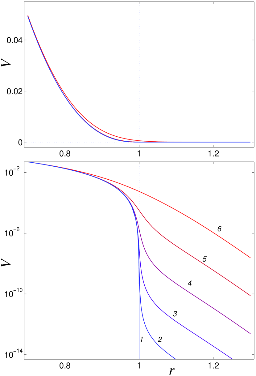
Figure 1: (Color online) Comparison between potential of interaction, given by formula (1) (curve 1) and smoothed potential $V_{h}(r)$, given by (2), for $h=0.000001$, 0.00001, 0.0001, 0.001, 0.01 (curves 2, 3, 4 ,5, 6), parameter $\alpha=5/2$.

To demonstrate that, we consider a chain of one-dimensional rods with the following purely repulsive potential of the nearest-neighbor interaction:

$$V(r) = 0,~{}~{}\mbox{for}~{}~{}r>D,$$

$$V(r) = V_{l}(r)=K|D-r|^{\alpha},~{}~{}\mbox{for}~{}~{}r\leq D,$$ (1)

Here $\alpha\geq 2$ – parameter that governs the growth of the repulsive force, $r$ is the distance between the centers of neighbor rods; $D$ is the size of the rod. The case $\alpha=2$ corresponds to semi-elastic rods considered in GS14 ; $\alpha=5/2$ corresponds to the case of Hertzian contact. Without restricting the generality, we further use non-dimensional parameters $D=1$, $K=1$. Then, the limit $\alpha\rightarrow\infty$ corresponds to the case of perfect instantaneous elastic collision as $r=1$.

In order to avoid numeric problems related to non-analyticity of potential (1) at $r=1$, we substitute it in the simulations by smoothed potential function

$$V_{h}(r)=2^{-\alpha}\left[\sqrt{\rho^{2}+hf(\rho)}-\rho\right]^{\alpha},~{}~{}\rho=r-1,$$ (2)

where function $f(\rho)=1/(1+5\rho^{2})^{6}$, parameter $h>0$. In the limit $h\rightarrow 0$ the smoothed potential (2) tends to non-analytic potential (1). Comparison between exact and smoothed potentials of interaction is presented in Fig. 1 for different values of the smoothing parameter $h$.

We perform traditional numeric simulation of the equilibrium heat transport in one-dimensional model and consider a segment of length $L$ parallel to $x$ axis. We pack $N=p(L-1)+1$ rods along this segment, where $p$ ($0<p<1$) stands for the packing ”density” of the chain. Fixed boundary conditions are imposed on both ends of the chain, i.e. $x_{1}\equiv 0$, $x_{N}\equiv(N-1)a$, where $a=1/p$ stands for the period of the unperturbed chain. Fixed boundaries enforce the density conservation. The disks $1<n<N$ are then restricted to move in $x$ direction. Hamiltonian of the chain in this case is expressed as

$${\cal H}=\sum_{n=2}^{N-1}\frac{1}{2}{x^{\prime}_{n}}^{2}+\sum_{n=1}^{N-1}V(x_{n+1}-x_{n}).$$ (3)

Here $\{x_{n}\}_{n=1}^{N}$ are coordinates of the rod centers.

To model the heat transfer along the chain under consideration, stochastic Langevin thermostats are used. The left end ($x<L_{0}=10$) of the chain is attached to the Langevin thermostat with temperature $T_{+}$, and the right end of the chain with the same length [$x>(N-1)a-L_{0}$] – to thermostat with temperature $T_{-}$. We adopt $T_{\pm}=(1\pm 0.05)T$, where $T$ is average temperature of the chain. The corresponding equations of motion have the following form:

$$x^{\prime\prime}_{n} = -\partial{\cal H}/\partial x_{n}-\gamma x^{\prime}_{n}+\xi_{n}^{+},~{}~{}\mbox{if}~{}~{}x_{n}<L_{0},$$

$$x^{\prime\prime}_{n} = -\partial{\cal H}/\partial x_{n},~{}~{}\mbox{if}~{}~{}L_{0}\leq x_{n}\leq(N-1)a-L_{0},$$ (4)

$$x^{\prime\prime}_{n} = -\partial{\cal H}/\partial x_{n}-\gamma x^{\prime}_{n}+\xi_{n}^{-},~{}~{}\mbox{if}~{}~{}x_{n}>(N-1)a-L_{0},$$

where $\gamma=0.1$ is a damping coefficient, $\xi_{n}^{\pm}$ is Gaussian white noise, which models the interaction with the thermostats, and is normalized as $\langle\xi_{n}^{\pm}(\tau)\rangle=0$, $\langle\xi_{n}^{+}(\tau_{1})\xi^{-}_{k}(\tau_{2})\rangle=0$, $\langle\xi_{n}^{\pm}(\tau_{1})\xi_{k}^{\pm}(\tau_{2})\rangle=2\gamma T_{\pm}\delta_{nk}\delta(\tau_{2}-\tau_{1})$.

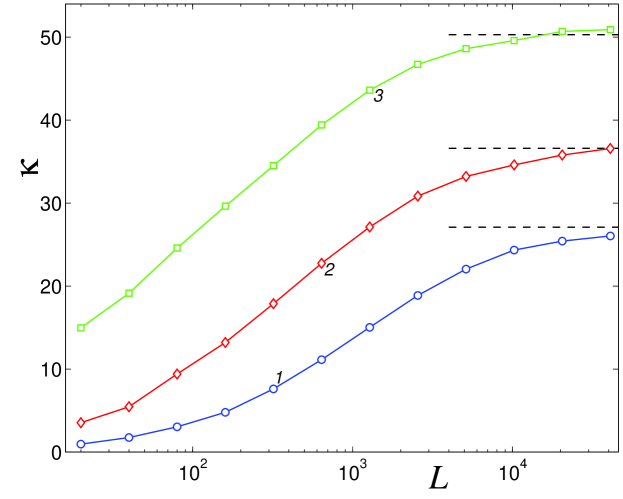
Figure 2: (Color online) Dependence of the heat conduction coefficient $\kappa$ on the distance between thermostats $L$ for temperatures $T=0.001$ (curve 1), 0.01 (curve 2), 0.1 (curve 3) and fixed density. The system includes rods with diameter $d=1$ with density $p=0.5$ (average distance between the rods $a=1/p=2$), power of potential function $\alpha=5/2$. Straight dashed lines correspond to the results obtained from Green-Kubo formula.

System of equations (4) with initial conditions ${\bf X}(0)=\{x_{n}(0)=(n-1)a,~{}x^{\prime}_{n}(0)=0\}_{n=1}^{N}$ was integrated numerically by Velocity Verlet method Verlet . Then, after some initial transient, a stationary heat flux $J$ and stationary local temperature distribution $T(x)$ are achieved.

The total heat flux $J$ was measured as the average work produced by the thermostats over unit time. For this sake, at each step of numerical integration $\Delta\tau$ new coordinates of the disks were calculated without account of the interaction with thermostats ${\bf X}_{0}(\tau+\Delta\tau)$ and then the same coordinates were calculated for chain interacting with the thermostats, denoted as ${\bf X}(\tau+\Delta\tau)$. We define $E_{+}$ as the energy of the leftmost segment of the chain which consists of disks with coordinates $x_{n}<L/2$ and $E_{-}$ as energy of the right most segment, where disks have coordinates $x_{n}>L/2$. Then the work done by the external forces in the time interval $[\tau,\tau+\Delta\tau]$ is expressed as

$$j_{\pm}=[E_{\pm}({\bf X}(\tau+\Delta\tau))-E_{\pm}({\bf X}_{0}(\tau+\Delta\tau))]/\Delta\tau.$$ (5)

By taking time average $J_{\pm}=\langle j_{\pm}\rangle_{\tau}$ we obtain the average value of energy flux-out from the left ”hot” thermostat and the average value of the energy flux-in into the right ”cold”  thermostat. The value of energy flux along the chain is $J=J_{+}=-J_{-}$. Accuracy of this balance is considered as one of criterions for validity of the numeric procedure.

The local heat flux, i.e. the energy flow from disk $n$ to the neighboring disk $n+1$, is defined as $J_{n}=\langle j_{n}\rangle_{\tau}$, where

$$j_{n}=(x_{n+1}-x_{n})(x^{\prime}_{n+1}+x^{\prime}_{n})F(x_{n+1}-x_{n})/2+x^{\prime}_{n}h_{n},$$

function $F(r)=-dV(r)/dr$, energy density distribution along the chain

$$h_{n}=[{x^{\prime}_{n}}^{2}+V(x_{n}-x_{n-1})+V(x_{n+1}-x_{n})]/2.$$

(see LLP03 ).

The thermal equilibrium requires all local fluxes to be equal to the total heat flux multiplied by the chain period, $J_{n}=aJ$. The fulfillment of this requirement may be considered as a criterion for stationary regime of the heat transport.

The local temperature distribution of the chain is calculated from kinetic energy of the rod. We divide the line segment $L$, which consists of $N$ disks, into unit-length cells $[i-1,i]$, $i=1,...,L$ and define the following quantities: the average number of disks in $i$-th cell is $\bar{n}_{i}$, and the average kinetic energy in the cell $\bar{E}_{i}$. Then the temperature of the cell is defined as $T(i)=2\bar{E}_{i}/\bar{n}_{i}$.

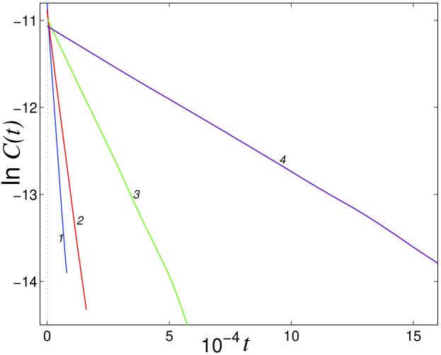
Figure 3: (Color online) Exponential decay of the autocorrelation function $C(t)$ for the chain of length $N=10000$ for temperature $T=0.033$ and density $p=0.25$, curves 1, 2, 3, 4 correspond to $\alpha=2$, 2.5, 4, 6 respectively.

Between the thermostats we observe linear temperature gradient $T(n)$ and constant thermal flux $J$. So, the heat conduction coefficient of the free fragment of the chain between the thermostats (of length $L-20$) can be estimated as follows:

$$\kappa(L)=J[T(11)-T(L-10)]/(L-20).$$ (6)

Well-known alternative way to evaluate the heat conduction coefficient is based on well-known Green-Kubo formula

$$\kappa=\lim_{\tau\rightarrow\infty}\lim_{N\rightarrow\infty}\frac{1}{NT^{2}}\int_{0}^{\tau}C(s)ds,$$ (7)

where $C(s)=\langle J_{tot}(t)J_{tot}(t-s)\rangle_{t}$ is autocorrelation function of the total heat flux in the chain with periodic boundary conditions $J_{tot}(t)=\sum_{n=1}^{N}j_{n}(t)$.

In order to compute the autocorrelation function $C(t)$ we consider a cyclic chain consisting of $N=10^{4}$ particles. Initially all particles in this chain are coupled to the Langevin thermostat with temperature $T$. After achieving the thermal equilibrium, the system is detached from the thermostat and Hamiltonian dynamics is simulated. To improve the accuracy, the results were averaged over $10^{4}$ realizations of the initial thermal distribution.

Numeric simulation of the thermalized cyclic chain of the disks had demonstrated that the autocorrelation function of the heat flux $C(t)$ decreases exponentially as $t\rightarrow\infty$ – see Fig. 3. Consequently, the integral in Green-Kubo formula (7) converges, yielding finite value for the HCC in the chain of the disks. Direct numeric simulation of the heat transport between the thermostats also yields saturation of $\kappa(L)$ for large values of $L$ – see Fig. 2. Both methods of simulation yield similar values of the HCC in the saturation regime.

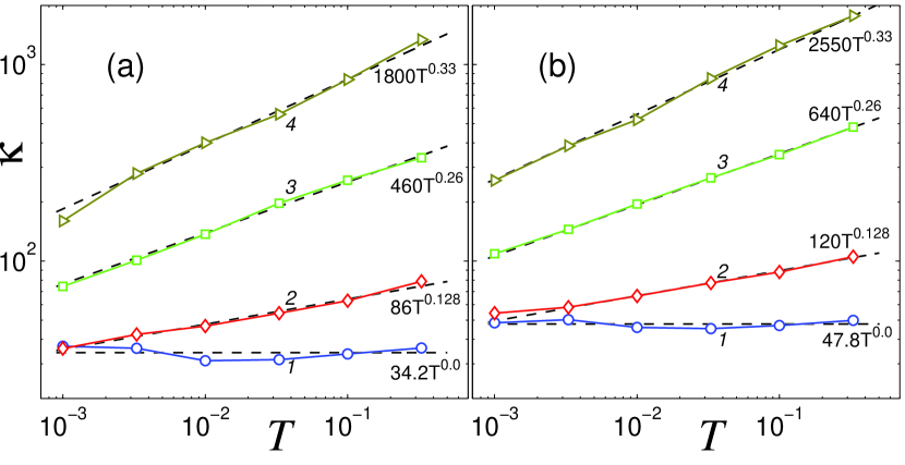
Figure 4: (Color online, double logarithmic scale) Temperature dependence of the HCC for (a) density $p=0.375$ and (b) $p=0.25$. Curves 1, 2, 3, 4 correspond to $\alpha=2$, 2.5, 4, 6 respectively. Straight dashed lines correspond to the power functions $\kappa=bT^{\beta}$.

As it was mentioned before, we hypothesize that the observed HCC saturation may be attributed to the triple collisions between the particles. To describe the transport process, it is convenient to define set of quasiparticles associated with the momenta of individual particles GS04 . The quasiparticles are not affected by the double collisions (the momenta just hop to the next particles), but are scattered by the triple collisions. Therefore, at phenomenological level, one can evaluate the HCC in terms of kinetic theory in the following way:

$$\kappa\sim c\lambda v\sim p\lambda v.$$ (8)

Here $v$ is the characteristic velocity of the quasiparticles, $c$ is heat capacity of the system, and $\lambda$ – the mean free path of the quasiparticles. Scattering events are related to triple collisions, so the mean free path corresponds to the distance traveled by the quasiparticle between such triple collisions:

$$\lambda\sim 1/pP_{tr},$$ (9)

where $P_{tr}$ is the probability that given collision is triple. This probability can be estimated as

$$P_{tr}\sim\tau_{c}/\tau_{f}.$$ (10)

Here $\tau_{f}$ is the time of flight between two successive collisions, and $\tau_{c}$ is the characteristic time of collision. One can also estimate $\tau_{f}\sim L/pv$ and therefore

$$\kappa\sim 1/p\tau_{c}.$$ (11)

Evaluation of the time of collision is simple due to finite range of interaction. If the particles collide with relative velocity $v_{0}$ at infinity, then the integral of energy for the two-particle system reads as

$$\frac{1}{2}\dot{x}^{2}+x^{\alpha}=\frac{1}{2}v_{0}^{2},$$ (12)

where $x(t)$ is the nonnegative relative displacement of the particles. Relative velocity becomes zero at the distance $x_{m}=(v_{0}^{2}/2)^{1/\alpha}$. The time of collision is presented as

$$\tau_{c}=2\int_{0}^{x_{m}}\frac{dx}{\sqrt{v_{0}^{2}-x^{\alpha}}}=$$

$$2^{1-1/\alpha}v_{0}^{2/\alpha-1}\int_{0}^{1}\frac{d\xi}{\sqrt{1-\xi^{\alpha}}},~{}~{}\xi=x/x_{m}.$$ (13)

Summarizing equations (10), (11), (13), and adopting $v_{0}\sim T^{1/2}$ one obtains:

$$\tau_{c}\sim v_{0}^{2/\alpha-1}\sim T^{1/\alpha-1/2}\Rightarrow\kappa\sim f(\alpha)p^{-1}T^{1/2-1/\alpha}$$ (14)

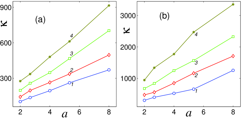
Figure 5: (Color online) Dependence of the HCC on inverse density $a=1/p$ for fixed temperature and (a) parameter $\alpha=4$ and (b) $\alpha=6$. Curves 1, 2, 3, 4 correspond to $T=0.01$, 0.033, 0.1, 0.33 respectively.

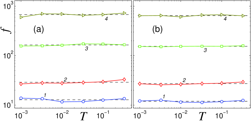
Figure 6: (Color online) Temperature dependence of the scaling function $f=p\kappa T^{1/\alpha-1/2}$ for (a) density $p=0.375$ and (b) $p=0.25$. Curves (1,2,3,4) correspond to $\alpha=2$, 2.5, 4, 6 respectively. Dashed straight lines correspond to the average values of $f$.

Equation (14) predicts two important features of the HCC in the considered model. First, it has nontrivial temperature dependence. Second, quite surprisingly, it is inversely proportional to the concentration of the particles.

Predictions for the scaling exponents in of simulations Equation (14) completely conform to the numeric results presented in Figures 4 and 5. In the same time, scaling function $f(\alpha)$ in (14) remains undetermined. We can suggest that it is completely governed by intricate dynamics of the three-particle collisions and thus depends solely on exponent $\alpha$. To verify that, we plot the function $f(\alpha)=\kappa pT^{1/\alpha-1/2}$ versus exponent $\alpha$. Numerical simulation demonstrates that the function $f(\alpha)$ does not depend on temperature $T$ and weakly depends on density $p$. – see Fig. 6. Figure 7 presents clear collapse of all available numeric data according to the above scaling function; the results suggest the power law $f\approx 1.12\alpha^{3.6}$. As expected, the HCC rapidly increases as power function of $\alpha$.

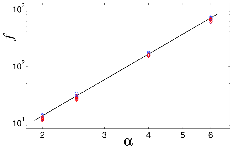
Figure 7: (Color online, double logarithmic scale) Dependence of the scaling function $f$ on power $\alpha$ for all simulated values of temperatures and particle densities. The data collapse on straight line corresponding to $f(\alpha)=1.12\alpha^{3.6}$.

For all explored values of $\alpha$ we observe the HCC saturation. Moreover, the observed scaling with concentration and temperature allows concluding that the observed saturation is caused by the triple particle collisions. Therefore, modification of the model and removal of unphysical instantaneous collisions lead to drastic modification of the transport properties – namely, the observed HCC saturation. As it was mentioned above, it is not possible to claim convergence in thermodynamic limit on the basis of numeric data for finite system. Still, we do not observe any trend towards ”resumed growth” of the HCC, similar to observed in the asymmetric FPU chain FPU-anti and billiard with alternating masses Casati . Of course, it might happen that simulations of even longer chains would demonstrate such growth also in the considered chain of stiff colliding particles. However, contrary to the asymmetric FPU and alternating-mass billiard, the considered model also allows clear and verifiable definition of basic kinetic parameters. The chains with possibility of dissociation possess similar property GS14 . Intuitively, as the mean free path can be defined, longer chains are expected to conform even better to the simple kinetic estimation of the heat conduction coefficient. Needless to say, this latter argument also does not prove anything, and further explorations are required to verify whether the considered model belongs to a universality class different from the FPU chain.

The authors are very grateful to Professor Stefano Lepri for useful discussions. The authors are grateful to Israel Science Foundation (grant 838/13) for financial support.

References

- (1) Fermi E., Pasta J. Ulam S, Los Alamos, Report No. LA-1940, 1955.
- (2) R. E. Peierls. Quantum Theory of Solids. Oxford University Press, Oxford, 1955.
- (3) Jackson E. A. Mistriotis A. D., J. Phys.: Condens. Matter, 1, 1223 (1989).
- (4) Gendelman O.V. and Manevitch L.I., Sov. Phys. JETP, 102, 511 (1992).
- (5) Lepri S., Livi R., and Politi A., Phys. Rev. Lett. 78, 1896 (1997).
- (6) Dhar A., Phys. Rev. Lett., 86, 3554 (2001).
- (7) Hatano T., Phys. Rev. E, 59, R1 (1999).
- (8) Casati G., Prosen T., Physical Review E 67, 015203 (2003).
- (9) Pereverzev A. Phys. Rev. E 68, 056124 (2003).
- (10) Narayan O., Ramaswamy S. Phys. Rev. Lett. 89, 200601 (2002).
- (11) S. Lepri, R. Livi, and A. Politi, Phys. Rep. 377, 1 (2003).
- (12) S.Lepri, R.Livi and A.Politi, in Thermal transport in low dimensions: from statistical physics to nanoscale heat transfer, ed. S.Lepri, Lecture Notes in Physics vol. 921, 2016.
- (13) Lippi A. and Livi R., J. Stat. Phys., 100, 1147 (2000).
- (14) Saito K. and Dhar A., Phys. Rev. Lett., 104, 040601 (2010).
- (15) Narayan O. and Ramaswamy S., Phys. Rev. Lett, 89, 200601 (2002).
- (16) Lukkarinen J. and Spohn H., Communications on Pure and Applied Mathematics, 61, 1753 (2008).
- (17) Delfini L., Lepri S., Livi R. and Politi A., Phys. Rev. E, 73, 060201(R) (2006).
- (18) van Beijeren H., Phys. Rev. Lett. 108, 180601 (2012).
- (19) Lee-Dadswell G.R., Phys. Rev. E 91, 012138 (2015).
- (20) Gendelman O. V. and Savin A. V., Phys. Rev. Lett., 84, 2381 (2000).
- (21) Giardina C., Livi R., Politi A. and Vassalli M., Phys. Rev. Lett., 84, 2144 (2000).
- (22) Zhong, Y., Zhang, Y., Wang, J. and Zhao, H., Phys. Rev. E 85, 060102 (2012).
- (23) Wang, L., Hu, B., Li, B., Phys. Rev. E 88 , 052112 (2013).
- (24) Savin A. V. and Kosevich Yu. A., Phys. Rev. E, 89, 032102 (2014).
- (25) Gendelman O. V. and Savin A. V., Europhysics Letters, 106, 34004 (2014).
- (26) Zolotarevskiy V., Savin A. V. and Gendelman O. V., Phys. Rev. E, 91, 032127 (2015).
- (27) Spohn, H., Journal of Statistical Physics 154, 1191 (2014).
- (28) Chen S., Wang J., Casati G., and Benenti G., Phys. Rev. E 90, 032134 (2014).
- (29) Gendelman O.V. and Savin A.V., Physical Review Letters, 92, 074301 (2004).
- (30) Dhar A., Adv. Phys. 57, 457 (2008).
- (31) Verlet L., Phys. Rev. 159, 98 (1967)