Modelling Geomechanical Impact of CO₂ Injection Using Precomputed Response Functions

Abstract

When injecting CO₂ or other fluids into a geological formation, pressure plays an important role both as a driver of flow and as a risk factor for mechanical integrity.

The full effect of geomechanics on aquifer flow can only be captured using a coupled flow-geomechanics model. In order to solve this computationally expensive system, various strategies have been put forwards over the years, with some of the best current methods based on sequential splitting.

In the present work, we seek to approximate the full geomechanical effect on flow without the need of coupling with a geomechanics solver during simulation, and at a computational cost comparable to that of an uncoupled model. We do this by means of precomputed pressure response functions. At grid model generation time, a geomechanics solver is used to compute the mechanical response of the aquifer for a set of pressure fields. The relevant information from these responses is then stored in a compact form and embedded with the grid model.

We test the accuracy and computational performance of our approach on a simple 2D and a more complex 3D model, and compare the results with those produced by a fully coupled approach as well as from a simple decoupled method based on Geertsma’s uniaxial expansion coefficient.

1 Introduction

1.1 Background

In order for carbon capture and storage (CCS) to play a significant role in the mitigation of climate change, hundreds or even thousands of megatonnes of would have to be injected annually into geological formations on a worldwide basis [8]. This represents a huge scale-up from current practice and experience, which means that we to a large extent need to rely on theoretical knowledge and computer simulations to gain insight into storage-related issues such as injectivity, capacity or long-term migration. Frequently, the use of computer models to investigate such questions will involve working with sparse or poorly constrained data, and address issues that relate to a wide range of spatial and temporal scales. The ability to run a large number of simulations in a reasonable amount of time is crucial, as it allows efficient exploration of different hypotheses and choices of parameters, evaluation of various injection scenarios and assessment of potential risk factors. Examples are workflows that include inverse modeling, optimization of storage operations, or risk analysis in the face of a large number of unknown or uncertain parameters. For this reason, the case for simplified tools for modeling CO₂ storage, less demanding than the use of traditional reservoir simulators, has previously been argued [28, 25]. Significant effort has been spent on the development of simplified tools for predicting subsurface flow of CO₂ at large scales. Over time, the capabilities of such tools have been expanded to account for a considerable range of physical phenomena [27, 16, 17, 26, 1]. However, reduced models that properly account for the two-way coupling between fluid flow and rock mechanics have so far received less attention, although recent work in this field includes the linear vertical deflection model of [5].

Geomechanical issues have proved to be important even in the context of current, limited size CO₂ storage operations [40, 12], and will be even more important to understand for the larger-scale operations envisioned in a global mitigation scenario. Potential geomechanical risks associated with CO₂ storage include seismicity, fault reactivation, rock fracturing and unwanted fluid displacement [33]. Understanding these risks will be important for any discussion regarding injectivity, storage capacity or long-term safety.

Investigating geomechanical effects requires the ability to model the interplay between fluid flow, pressure, mechanical stresses and strains, as well as the impact of deformation on rock properties. The theoretical framework of poromechanics was first introduced in the forties by the work of Karl von Terzaghi and Maurice Biot. Significant attention has later been paid to how this framework can be applied to reservoir engineering, and how the resulting system of coupled equations describing pressure and mechanical displacement can be efficiently solved [37, 36, 22, 11, 19, 23, 18].

A significant number of studies have been carried out on the topic of geomechanics and CO₂ injection over the years. At the theoretical level, the poromechanical framework has been used to investigate the risk of fracturing or fault slip caused by elevated pressure and reduced effective stress [34, 32, 6], and assess the risk of induced seismicity [7]. A reduced model for coupled flow and geomechanics, adapted to the case of CO₂ storage, was proposed by [5], whereas [9] situates geomechanics within a comprehensive modeling framework for CO₂ storage, where different physical processes are modeled depending on the spatial and temporal scale. Specific case-studies involving CO₂ injection and geomechanical impacts include Ketzin [29], In-Salah [35, 30, 4], Vedsted [39] and the CO2CRC Otway Project [2].

When fluid is injected into a geological formation, the resulting change in underground pore pressure is accompanied by some degree of mechanical deformation of the rock matrix caused by a change in the underground balance between mechanical and pressure forces. The rock deformation also has an impact on the evolution of the pressure field itself, as the expansion or contraction of the rock matrix modifies material parameters that affect fluid flow, in particular porosity and permeability [10]. Whereas the influence of pressure on rock deformation is fundamental in any combined simulation of geomechanics and fluid flow, the impact of geomechanics on the pressure field is often simplified or neglected. In reservoir modeling, the most common practice is to simulate reservoir flow in isolation, and compute the corresponding mechanical deformation as a post-processing step if desired. Under this approach, the full impact of rock mechanics on fluid flow is not explicitly modeled, but the effect is approximated by making rock properties (typically linear) functions of local pressure or assumed stress. In particular, the effect of rock expansion is frequently modeled using a pore volume compressibility coefficient, which affects the accumulation term of the governing mass-balance equations [37, 11, 22]. This approach is standard practice in most commercial and academic reservoir simulation software, and is often considered to provide a perfectly adequate approximation of the real behavior of the poromechanical system. In the context of geomechanics and CO₂ storage, it has been utilized in e.g. [29, 2, 39].

On the other hand, a full account of geomechanical effects requires explicit modeling of the two-way coupling between the flow and mechanical subsystems. This requires embedding the reservoir simulation grid within a larger mechanical grid that includes the over- and underburden, and solving the equations of the combined system together. In this setting, flow is frequently restricted to the reservoir part of the model, whereas mechanical deformations occur throughout the model.

Under the fully coupled approach, each discrete element (node, face or cell, depending on the numerical discretization) in the mechanical model comes with three displacement unknowns that must be solved for, alongside with the unknowns of the flow equation. The full flow/mechanical system is thus described by two coupled equations of elliptic character. All in all, this leads to a numerical model with a large number of unknowns, which is computationally heavy to solve. Various strategies based on sequential splitting have been proposed for computing the solution in an efficient manner, e.g. [36, 22, 11], and the “fixed-stress split” approach has been shown to have particularly favorable convergence properties [19, 23]. In addition to being attractive from a computational viewpoint, sequential splitting approaches have the additional advantage that they allow flow and mechanics equations to be separately addressed by standard solvers that have been highly adapted to their specific fields over the years. Examples where fully coupled geomechanical modeling has been used in the context of CO₂ storage include [34], [9] and [30].

The general need for fully coupled models versus the more common practice of one-way coupling has been argued both ways in the past in the context of aquifer pumping and subsidence problems [21, 14]. Regarding CO₂ injection, the geomechanical feedback on fluid flow was observed to be weak and localized around the injection well for the test cases explored in [9]. In any case, there seems to be a general recognition in the research community that the full geomechanical impact on flow is of relevance in some situations, as brought to witness by the significant amount of related research activity in recent years.

1.2 Our proposed approach

Sequential splitting strategies in combination with iterative linear solvers can provide a significant gain in computational efficiency compared to solving all equations as a single system. However, they remain significantly more expensive than modeling aquifer flow in isolation, as is common practice in reservoir engineering. This is because the sequential splitting approach still requires the mechanics equations to be solved repeatedly throughout the simulation. In the case of iterative strategies, both the flow and mechanics equations have to be solved multiple times for every timestep until convergence is achieved. Moreover, even though the splitting approach permits the flow simulator and geomechanics solver to be chosen independently, it is still necessary to have access to both types of software at runtime.

In the approach we propose in this paper, we aim to include the full effect of geomechanics on fluid flow to different degrees of approximation, without the need of a mechanics solver at simulation time. As such, the computational requirement of a flow simulation becomes comparable to that of standard reservoir modeling, but can still reproduce the solution obtained from solving the two-way coupled system. This advantage comes at the expense of a precomputation step at grid generation time, where the mechanical responses of the grid for a large set of discrete pressure fields are determined and stored for re-use at flow simulation time. The approach is based on the theory of linear poroelasticity [41]. Its practical feasibility relies on the observation that although a local change in a pressure field can have significant non-local mechanical effects in terms of displacements, the impact on rock expansion (i.e. the divergence of displacements), is typically much more local in the case of boundary conditions relevant to CO₂ injection, as will be discussed in the next section.

For simplicity, our focus is limited to one-phase flow, although the proposed method is trivially extendable to multi-phase flow under the assumption that mechanical response is tied to effective fluid pressure. Also, we have omitted the impact of geomechanical stress on rock permeability. This effect could also be easily included in the model, but merits a separate analysis and is thus considered future work.

2 Conceptual system, theory and basic idea

We consider a fluid injection or extraction operation into/out from a subterranean reservoir or aquifer. We neglect fluid flow through aquifer top and bottom boundaries, and impose either no-flow or fixed pressure along lateral boundaries. To model mechanical deformation, the aquifer model is embedded in a larger rock matrix that includes the over- and underburden (collectively referred to as the surrounding domain). The overburden zone extends up to the surface, where the mechanical boundary condition is that of fixed, normal traction, while the underburden zone extends down to some specified deeper level where zero mechanical displacements are assumed. The lateral boundary conditions can be of any type; for the purpose of the examples presented in this paper, we use the ‘roller’ type with zero lateral displacements and constant vertical stress.

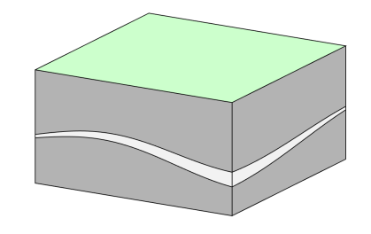
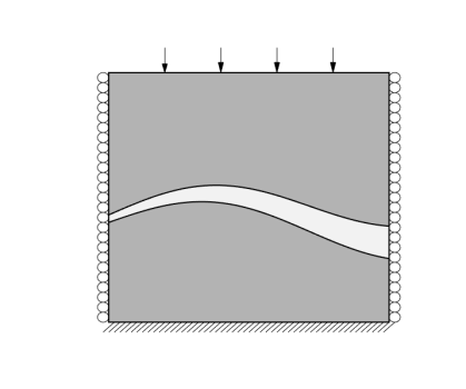
Figure 1: Left: The conceptual model. The aquifer is illustrated as a light band within a darker matrix of surrounding rock that extends up to the ground level (green surface). Fluid flow only takes place in the aquifer, whereas mechanical deformations are computed for the full model. Right: Cross-section view of the model, with mechanical boundary conditions indicated. Lateral boundaries can be of any type (‘roller’ type indicated on figure).

The complete model domain is denoted $\Omega$, with boundary $\partial\Omega$. The domain $\Omega$ is subdivided in two separate zones, the aquifer $\Omega_{aq}$ and the surrounding domain $\Omega_{sd}$. For simplicity, we model $\Omega_{aq}$ and $\Omega_{sd}$ as having separate but spatially invariant sets of poroelastic moduli. As the modeling of fluid flow is restricted to the aquifer, the associated pressure field is only defined on $\Omega_{aq}$. Accordingly, drained poroelastic moduli are used to describe $\Omega_{aq}$, whereas $\Omega_{sb}$ is described in terms of undrained moduli. We thereby neglect the effect of pressure changes and flow occurring outside the aquifer as a result of mechanical deformations induced by the pressure field inside the aquifer. A basic, layered structure similar to Figure 1 is assumed, but $\Omega_{aq}$ and $\Omega_{sd}$ can be of arbitrary geometrical shape and topology, including pinch-outs.

2.1 Linear poroelasticity formulation

Since mechanical deformations are expected to remain small and mechanical equilibrium assumed to be reached on a time scale much shorter than that of fluid flow, we model the coupled flow-mechanical system within the framework of linear poroelasticity. The governing equations then consist of the force equilibrium equations for mechanics and an inhomogeneous diffusion equation for fluid pressure. Coupling between equations arise as the gradient of pore pressure plays the role as a body force in the mechanical equilibrium equations, whereas mechanical strain appears in the accumulation term of the pressure diffusion equation. In our formulation, the independent unknown variables consist of the mechanical displacement field $\textbf{u}=[u_{x},u_{y},u_{z}]^{T}$ defined on $\Omega$, and the fluid pressure $p$ defined on $\Omega_{aq}$.

The mechanical system is assumed to be in translational and rotational equilibrium at any time. Rotational equilibrium implies that the total stress tensor, $\bm{\sigma}$, should be symmetrical, i.e.:

$$\bm{\sigma}=\bm{\sigma}^{T}$$ (1)

whereas translational equilibrium requires that the divergence of this tensor counterbalances the body forces F acting on it:

$$\nabla\cdot\bm{\sigma}+\textbf{F}=0$$ (2)

In linear poroelasticity, provided tensile stresses are taken to be positive, total stress equals the difference between effective stress $\bm{\sigma}^{\prime}$ and a term proportional to fluid pressure:

$$\bm{\sigma}=\bm{\sigma}^{\prime}-\alpha p\textbf{I}$$ (3)

where $\alpha$ is the Biot-Willis coefficient and I is the identity matrix in $\mathbb{R}^{3}$. Effective stress is linked to elastic strain $\bm{\epsilon}$ through Hooke’s law:

$$\bm{\sigma}^{\prime}=\textbf{C}\bm{\epsilon}$$ (4)

where C is the fourth-order elasticity tensor, and the elastic strain tensor $\bm{\epsilon}$ is defined as:

$$\bm{\epsilon}=\frac{1}{2}(\nabla\textbf{u}+\nabla\textbf{u}^{T})$$ (5)

For an isotropic material, (4) reduces to:

$$\bm{\sigma}^{\prime}=2G\bm{\epsilon}+(K-\frac{2}{3}G)\text{tr}({\bm{\epsilon}})\textbf{I}$$ (6)

where $K$ and $G$ denote respectively the drained bulk and shear moduli of the material, and $\text{tr}(\bm{\epsilon})$ denotes the trace of $\bm{\epsilon}$. $K$ and $G$ can be space-dependent. By combining the equilibrium equation (2) with (3), (5) and (6), we obtain the displacement formulation of the force balance equation for an isotropic material:

$$\nabla\cdot(G\nabla\textbf{u})+\nabla\left((K+\frac{1}{3}G)\nabla\cdot\textbf{u}\right)-\alpha\nabla p=\rho_{b}\textbf{g}$$ (7)

Here, we have considered that the body force F from (2) consists of the gravity force only, i.e. $\textbf{F}=-\rho_{b}\textbf{g}$, where $\rho_{b}$ is the bulk density of the medium and g is gravitational acceleration.

In addition, boundary conditions must be specified. Boundary conditions can be of different type for different spatial components of the displacement vector u. For instance, lateral roller boundary conditions specify zero displacement (Dirichlet) for $u_{x}$ and $u_{y}$, but fixed-stress (Neumann) for $u_{z}$. Each spatial component $i\in{\{x,y,z\}}$ of u thus has its own subdivision of $\partial\Omega$ into a Neumann ($\Gamma_{t}^{i}$) and a Dirichlet ($\Gamma_{g}^{i}$) part. For each spatial component $i$, fulfillment of the boundary conditions requires:

$$u_{i} =g_{i}\text{ on }\Gamma^{i}_{g}$$ (8)

$$\sigma_{ji}n_{j} =t_{i}\text{ on }\Gamma^{i}_{t}$$ (9)

Regarding rotational equilibrium, from (3), (5) and (6) it is easy to see that the symmetry requirement of (1) is automatically fulfilled.

The pressure equation governing single-phase fluid flow is obtained by combining the fluid continuity equation with Darcy’s constitutive relationship between pressure and flow. The fluid continuity equation with volumetric source term $Q$ can be written:

$$\dot{\zeta}+\nabla\cdot\textbf{q}=Q$$ (10)

Here, q represents the volumetric fluid flux and $\zeta$ denotes the accumulation term. In poroelastic literature, starting with [3], $\zeta$ is commonly referred to as the increment of fluid content, and represents the volume of fluid imported into a control volume, per control volume. It is modeled as depending linearly on fluid pressure $p$ and volumetric strain $\epsilon=\text{tr}(\bm{\epsilon})=\nabla\cdot\textbf{u}$, so that the time derivative becomes:

$$\dot{\zeta}=\frac{\partial\zeta}{\partial p}\dot{p}+\frac{\partial\zeta}{\partial\epsilon}\dot{\epsilon}=S_{\epsilon}\dot{p}+\alpha\dot{\epsilon}$$ (11)

Here $S_{\epsilon}$ is called the specific storage coefficient at constant strain and $\alpha$ is the Biot-Willis coefficient that was already introduced in (3). The following expression can be derived for $S_{\epsilon}$ [41]:

$$S_{\epsilon}=\frac{1}{K}(1-\alpha)(\alpha-\phi)+\frac{\phi}{K_{f}}$$ (12)

Here, $\phi$ is the porosity of the medium and $\frac{1}{K_{f}}$ represents fluid compressibility.

The flux q is linked to the fluid pressure through Darcy’s law:

$$\textbf{q}=-\frac{k}{\mu}(\nabla p-\rho_{f}\textbf{g})$$ (13)

where $k$ is the permeability of the medium, $\mu$ represents fluid viscosity and $\rho_{f}$ fluid density. Combining Darcy’s law with (10) and (11), we obtain the pressure equation for single-phase flow:

$$\alpha\dot{\epsilon}+S_{\epsilon}\dot{p}-\nabla\cdot\frac{k}{\mu}(\nabla p-\rho_{f}\textbf{g})=Q$$ (14)

In our model, this equation governs fluid flow in $\Omega_{aq}$. Fluid flow is neglected in $\Omega_{sd}$, where we instead use the undrained bulk modulus $K_{u}=K+\frac{\alpha^{2}}{S_{\epsilon}}$, and the corresponding force balance equation reduces to that of linear elasticity.

The combined poroelastic equation system, with u and $p$ as unknowns, becomes:

$$\nabla\cdot(G\nabla\textbf{u})+\nabla\left((K+\frac{1}{3}G)\nabla\cdot\textbf{u}\right)-\alpha\nabla p=\rho_{b}\textbf{g}\;\;\; \text{ in }\Omega_{aq}$$ (15)

$$\nabla\cdot(G\nabla\textbf{u})+\nabla\left((K_{u}+\frac{1}{3}G)\nabla\cdot\textbf{u}\right)=\rho_{b}\textbf{g} \text{ in }\Omega_{sd}$$ (16)

$$\alpha\dot{\epsilon}+S_{\epsilon}\dot{p}-\nabla\cdot\frac{k}{\mu}(\nabla p-\rho_{f}\textbf{g})=Q \text{ in }\Omega_{aq}$$ (17)

Poroelastic parameters are here allowed to be spatially heterogeneous. In particular, they may vary between the aquifer and its surroundings, or between different geological layers. We see that (15) is coupled to (17) through the term $\alpha\nabla p$, whereas (17) is coupled to (15) and (16) through the term $\alpha\dot{\epsilon}$ $(=\alpha\nabla\cdot\dot{\textbf{u}})$.

Mechanical boundary conditions at $\partial\Omega$ are given by (8). Material continuity dictates the boundary conditions at the interfaces between $\Omega_{aq}$ and $\Omega_{sd}$. Boundary conditions for flow in $\Omega_{aq}$ are:

$$p =p^{0}\text{ on }\Gamma_{p}\;\;\;$$ (constant pressure) (18)

q $$=0\text{ on }\Gamma_{\textbf{q}}\;\;\;$$ (no-flow) (19)

where it is understood that the top and bottom boundaries of the aquifer are both part of $\Gamma_{\textbf{q}}$.

2.2 timestepping and linear system

A backwards-Euler time discretization of (17) yields:

$$\alpha\nabla\cdot\bm{u^{n+1}}+S_{\epsilon}p^{n+1}-\Delta t\frac{K}{\mu}\nabla^{2}p^{n+1}=\Delta tQ^{n+1}+\alpha\nabla\cdot\bm{u^{n}}+S_{\epsilon}p^{n}$$ (20)

where $\Delta t$ is the timestep size, and $(\textbf{u}^{n},p^{n})$ and $(\textbf{u}^{n+1},p^{n+1})$ are the values of $(\textbf{u},p)$ at timestep $n$ and $n+1$ respectively. Given an applicable spatial discretization scheme, the resulting linear system can be expressed as:

$$\begin{bmatrix}\textbf{G}&\textbf{S}+\Delta t\textbf{P}\end{bmatrix}\begin{bmatrix}\textbf{u}^{n+1}\\ p^{n+1}\end{bmatrix}=\begin{bmatrix}\textbf{G}&\textbf{S}\end{bmatrix}\begin{bmatrix}\textbf{u}^{n}\\ p^{n}\end{bmatrix}+\Delta t\textbf{Q}$$ (21)

where G is a discretization of $\alpha\nabla\cdot\textbf{u}$ restricted to aquifer cells, S is a discretization of $S_{\epsilon}p$, P is a discretization of $\frac{K}{\mu}\nabla^{2}p$ and Q is a discretization of the source term $Q$. If we moreover use M to represent a discretization of $\nabla\cdot(G\nabla\textbf{u})+\nabla\left((K+\frac{1}{3}G)\nabla\cdot\textbf{u}\right)$ and $\textbf{F}_{u}$ to represent a combined discretization of body forces $\rho_{b}\textbf{g}$ and boundary forces t, we get the linear system for the complete poroelastic problem:

$$\begin{bmatrix}\textbf{M}&\textbf{G}^{T}\\ \textbf{G}&\textbf{S}+\Delta t\textbf{P}\end{bmatrix}\begin{bmatrix}\textbf{u}^{n+1}\\ p^{n+1}\end{bmatrix}=\begin{bmatrix}\textbf{0}&\textbf{0}\\ \textbf{G}&\textbf{S}\end{bmatrix}\begin{bmatrix}\textbf{u}^{n}\\ p^{n}\end{bmatrix}+\begin{bmatrix}\textbf{F}_{u}\\ \Delta t\textbf{Q}\end{bmatrix}$$ (22)

Since the gradient operator is the negative adjoint of the divergence operator away from the boundary, the discretization of $\alpha\nabla p$ is here $-G^{T}$. It is assumed that the matrices M, S and P are symmetrical.

It is worth noting that the number of aquifer cells in a discrete model, $N_{aq}$, is usually significantly less than the total number of cells in the model $N=N_{aq}+N_{sd}$. Moreover, since pressure is scalar whereas u has 3 components (in 3D), the number of discrete values $u_{i}$ is approximately $3N$, whereas the number of discrete values $p_{i}$ is only about $N_{aq}$. As a consequence, the square matrix M is much larger than $\textbf{S}+\Delta t\textbf{P}$ and G, and the system block matrix takes on the following shape:

M	$\textbf{G}^{T}$
G	$\textbf{S}+\Delta t\textbf{P}$

Another important observation is that the influence of the displacement field u on the pressure equation is only in terms of its divergence $\epsilon$. As we argue in the next subsection, the impact of a local pressure change on $\epsilon$ is generally localized, even though the influence on u can be far-reaching. This is key to the practicality of our proposed method when applied to large models.

Finally, we note that if one were to eliminate u from (22) using the Schur complement, we define $\textbf{E}=-\textbf{G}\textbf{M}^{-1}\textbf{G}^{T}$ and obtain:

$$(\textbf{E}+\textbf{S}+\Delta t\textbf{P})p^{n+1}=(\textbf{E}+\textbf{S})p^{n}+\Delta t\textbf{Q}$$ (23)

The matrix $\textbf{E}\in\mathbb{M}_{N_{aq}}$ here represents volumetric strain $\epsilon$ as a function of $p$ only. It is a symmetric matrix whose size is significantly smaller than the full system matrix ($\mathbb{M}_{3N+N_{aq}}$). On the other hand, E is non-sparse, making it impractical to store and invert directly. As becomes apparent in the discussion of our method below, our approach can be numerically interpreted as the use of a truncated form of the Schur complement.

2.3 Decoupled flow simulation and Geertsma’s uniaxial poroelastic expansion coefficient

Under the assumption of zero lateral strain and constant vertical stress, the pressure equation (17) completely uncouples from the mechanical equations (15) and (16) [41]. With this assumption, which is often made in hydrogeology, changes in local strain $\Delta\epsilon$ become directly proportional to changes in local pressure $\Delta p$ through the relation:

$$\Delta\epsilon=c_{m}\Delta p$$ (24)

The factor $c_{m}$ is called Geertsma’s uniaxial poroelastic expansion coefficient. It is related to the elastic moduli $K$ and $G$ as follows:

$$c_{m}=\frac{\alpha}{K_{v}}$$ (25)

where $K_{v}=K+\frac{4}{3}G$ is the (drained) uniaxial bulk modulus of the material. By combining (24) with (17), we obtain the uncoupled pressure equation:

$$(\alpha c_{m}+S_{\epsilon})\dot{p}-\frac{K}{\mu}\nabla^{2}p=Q$$ (26)

The only unknown in this equation is pressure. This is equivalent to the standard transient flow equation used in hydrogeology:

$$S\dot{p}-\frac{K}{\mu}\nabla^{2}p=Q$$ (27)

where $S=\alpha c_{m}+S_{\epsilon}$ is the uniaxial specific storage parameter. Combining (26) with the expression for $S_{\epsilon}$ in (12), we see that $S$ can be divided into two parts $S=S_{1}+S_{2}$, where $S_{1}=\alpha c_{m}+\frac{1}{K}(1-\alpha)(\alpha-\phi)$ accounts for rock expansion and grain compressibility, whereas $S_{2}=\frac{\phi}{K_{f}}$ accounts for fluid compressibility. Such a presentation of the accumulation term is frequently made in commercial and academic reservoir simulation code (although not necessarily derived in the same way), where the equivalent of $S_{1}$ is interpreted as a pore volume compressibility coefficient, and $S_{2}$ can be easily generalized to the nonlinear case where fluid density is obtained from an equation of state.

We refer to this decoupled approach, popular in reservoir modeling, as the local model, since the relationship between aquifer volumetric strain and pressure (24) is completely local. After solving for pressure using (26), mechanical displacements can be subsequently obtained using (15) and (16), in which case it can be considered a one-way coupled approach.

As demonstrated in the next section, the local model often produces good results despite its simplicity and low computational requirements. Nevertheless, it is clear that the assumption of zero lateral strain can be only approximately true throughout a problem domain. The assumption breaks down in the presence of strong lateral pressure gradients, e.g. in the vicinity of injecting or producing wells. The model’s tendency to produce good results even in the presence of strong pressure gradients can also be understood through a different interpretation. As shown in the Appendix, the analytical solution of (7) in an infinite domain with constant elastic moduli leads to relation (24) without any further assumptions on stresses and strains. In other words, any changes in strain that are non-locally dependent on pressure must in some way be related to material heterogeneities and/or influence from the imposed boundary conditions. (For instance, if the system as a whole is not allowed to expand, internal changes in volume would always be zero-sum, so a local expansion of a given internal volume would necessarily have non-local impact). In any case, as the system tends towards steady state, the time-dependent term in (17) vanishes and the flow and mechanical systems decouple, in which case (17) and (27) become equivalent.

Since $c_{m}$ is derived from the assumption of zero lateral strain, it represents the increase in pore volume resulting from a uniform vertical expansion of the aquifer, as would approximately result from a uniform pressure increase throughout the aquifer domain. This means that we can use our poroelastic formulation to compute a numerical generalization of $c_{m}$, which we note $\bar{c}_{m}$, and which can account for arbitrary boundary conditions and heterogeneous rock parameters. This is done by solving the elastic equations (15), and (16) a single time for $p$ equal to a uniform, unit pressure increase, and using the obtained displacement field to compute the corresponding volumetric strain $\epsilon$ for each individual aquifer cell. An example is presented in Figure 2, where we have computed $\bar{c}_{m}$ using a 2D (x, z) model of a horizontal aquifer embedded in a larger rock matrix, at a depth of 950 m. The aquifer is 10 km long and 100 m thick, and the poroelastic parameters are $\alpha=0.9$, $K_{aq}=10^{9}$, $G_{aq}=8\times 10^{8}$, $K_{sd}=1.3\times 10^{11}$ and $G_{sd}=1.4\times 10^{10}$. We plot $\Delta\epsilon/\Delta p$ for two different specified lateral boundary conditions, and compare with the theoretical value of $c_{m}$. With roller boundary conditions, $\bar{c}_{m}$ here reproduces the theoretical value of $c_{m}$, whereas clamped boundaries leads to strong variation of $\bar{c}_{m}$ towards the lateral boundaries, reflecting the local breakdown of the assumption of zero lateral strain and constant vertical stress. The numerically obtained parameter $\bar{c}_{m}$ is thus able to model more general boundary conditions than the underlying assumptions behind the analytical parameter $c_{m}$ suggests. As an extreme example, $\bar{c}_{m}$ would equal zero for a materially uniform domain constrained with zero-displacements on all sides. Material heterogeneities are also taken into account in the numerical value of $\bar{c}_{m}$.

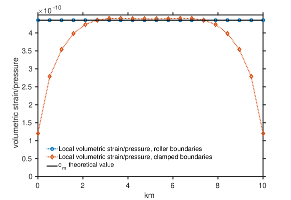
Figure 2: Numerical estimation of Geertsma’s uniaxial poroelastic expansion coefficient $c_{m}$ for a two-dimensional (x, z) flat and horizontal aquifer. The x-axis represents spatial position along the aquifer, whereas the y-axis represents the local change in volumetric strain for a unit, global pressure increase throughout the aquifer domain.

2.4 The use of precomputed response functions

The local model just described relies on simplifying assumptions that are at best approximately true, and fails to capture non-local relations between pressure and volumetric strain. On the other hand, solving the fully coupled linear poroelastic system represented by (22) quickly becomes computationally demanding. We here seek to establish a method that retains much of the computational efficiency of the local model, that does not require any assumptions on strains or stresses, and that is capable of producing results that are close to those obtained by a fully-coupled model.

The force balance equation of linear poroelasticity (7) establishes a relation between displacement field u, pressure $p$, body force $\textbf{F}=\rho\textbf{g}$ and boundary conditions bc, such that we can consider u to be uniquely determined from the others:

$$\textbf{u}=\textbf{u}(p,\textbf{F},\textbf{bc})$$ (28)

Moreover, as (7) is linear, the superposition principle applies. As such, if $p^{0}$ represents initial pressure and $p=p^{0}+\tilde{p}$ is a different pressure, we have:

$$\textbf{u}(p,\textbf{F},\textbf{bc})=\textbf{u}(p^{0},\textbf{F},\textbf{bc})+\textbf{u}(\tilde{p},0,0)$$ (29)

where $\textbf{u}(p^{0},\textbf{F},\textbf{bc})$ represents initial deformation. Assuming body forces and boundary conditions remain constant, we can directly relate a change in displacements ${\bm{\tilde{u}}=\textbf{u}(p,\textbf{F},\textbf{bc})-\textbf{u}(p^{0},\textbf{F},\textbf{bc})}$ to a change in pressure $\tilde{p}$:

$$\bm{\tilde{u}}=\textbf{u}(\tilde{p},0,0)$$ (30)

When solving a discretized system based on (7), the pressure field is defined using a linear combination of a set of basis functions $\{\phi_{1},...\phi_{M}\}$ and can be written: $p(\textbf{x})=\sum_{i=1}^{M}p_{i}\phi_{i}(\textbf{x})$. Using the notation $\tilde{p}_{i}=p_{i}-p_{i}^{0}$, the superposition principle allows us to write:

$$\bm{\tilde{u}}=\sum_{i=1}^{M}\tilde{p}_{i}\bm{u}(\phi_{i},0,0)$$ (31)

The corresponding change in volumetric strain $\tilde{\epsilon}=\nabla\cdot\bm{\tilde{u}}$ can thus be expressed:

$$\tilde{\epsilon}=\sum_{i=1}^{M}\tilde{p}_{i}\Psi_{i}$$ (32)

where $\Psi_{i}=\nabla\cdot\bm{u}(\phi_{i},0,0)$ represents the system’s volumetric strain response to pressure perturbation $\phi_{i}$. This means that knowledge of the set of (scalar) functions $\{\Psi_{1},...\Psi_{M}\}$ enables us to insert (32) into (17) to obtain an equation that only depends on pressure. This equation can then be solved decoupled from (15) and (16), while still providing the same pressure solution as the fully-coupled equation system.

In the context of volumetric strain, we will refer to the pressure basis functions $\{\phi_{i}\}_{i=1...M}$ as impulse functions and $\{\Psi_{i}\}_{i=1...M}$ as response functions. Our proposed approach consists of precomputing and storing a set of approximated volumetric strain response functions that corresponds to our set of pressure basis functions. At simulation time, we can then solve (17) using (32) to eliminate volumetric strain from the equation.

For the purpose of solving the pressure equation (17) of our model problem, we only need the values of the response functions $\{\Psi_{i}\}_{i=1...m}$ restricted to $\Omega_{aq}$. As the number of aquifer grid cells in $\Omega_{aq}$ is generally much lower than the total number of cells in $\Omega$, this allows us to cut down significantly the amount of information that must be precomputed and stored. A natural choice for the set of impulse functions $\{\phi_{i}\}$ is to let $\phi_{i}$ represent a unit pressure increase limited to aquifer grid cell $i$. However, for the examples given in the following section, a coarser set of impulse functions has been chosen, where $\phi_{i}$ represents an unit pressure increase in an entire vertical column of aquifer cells. This particular choice relies on the assumption that overpressure does not vary in a significant way across the vertical thickness of the aquifer. Given the large horizontal-to-vertical aspect ratio of a typical aquifer, we find that this approximation tends to work well in practice, while cutting back on the required amount of precomputation work.

In principle, the support of each response function $\Psi_{i}$ covers the entire $\Omega_{aq}$. However, for the physical conditions relevant to injection scenarios, in particular the presence of a free-moving top (land or sea) surface, $\Psi_{i}$ decays relatively quickly away from the support of the corresponding impulse $\phi_{i}$. This means it can be truncated at some distance beyond which its value falls below some defined threshold. The remaining function $\tilde{\Psi}_{i}$ has local support, and can be rescaled so that $\int_{\Omega_{aq}}\tilde{\Psi}_{i}dx=\int_{\Omega_{aq}}\Psi_{i}dx$. It is worth noting that if $\phi_{i}$ represents a unit pressure increase in cell $i$ and $\Psi_{i}$ is discretized as a cell-wise constant function, then necessarily $\int_{\Omega_{aq}}\Psi_{i}dx=\bar{c}_{m,i}$, where $\bar{c}_{m,i}$ is the value of $\bar{c}_{m}$ for cell $i$, as explained in the Appendix. As such, the truncated form $\tilde{\Psi}_{i}$ represents some intermediary between the fully cell-restricted coefficient $\bar{c}_{m}$ and the function with full global support $\Psi_{i}$, where all three entities represent the same total amount of aquifer volumetric strain.

As a consequence, the use of $\bar{c}_{m}$ in combination with the previously described local model can be understood as a limit case of using precomputed responses with a sufficiently high threshold, so that the full support of $\tilde{\Psi}_{i}$ falls within a single cell. However, in this case we know that the value of $\bar{c}_{m}$ for each and every aquifer cell can be determined by solving equations (15) and (16) once, as previously explained. Therefore, the required amount of precomputation is much less for this limit case.

A sample response function computed for a 2D model is presented in Figure 3. We here plot the height-averaged volumetric strain response as a function of lateral distance from a unit pressure perturbation (1 Pa) in a 100 meter thick, horizontal aquifer at a depth of 1000 meters. The aquifer consists of soft rock with a Young’s modulus value of 1 GPa, embedded in a stiffer rock with a Young’s modulus value of 10 MPa. A high resolution is used (10 m size grid blocks) in order to produce visually smooth curves. Comparing the red and blue curves, it is clear that the response function looks quite different depending on whether a single or ten layers were used in the vertical discretization of the aquifer region. This is because the full mechanical effect of the pressure perturbation cannot be properly captured without multiple vertical cell layers. Using multiple different sets of input parameters, we observe that response functions generally consist of an inner negative part followed by a local positive maximum, and finally an attenuation region where the response decays towards zero. These qualitative features can be explained as resulting from the counteracting effects of arching and bulging. The arching effect is produced by the elevated pressure of the impulse region pushing vertically against the over- and underburden regions, forcing them apart and causing nearby aquifer regions to expand (Figure 4, left). This effect becomes more spatially spread out for higher stiffness ratios between the surrounding domain and the aquifer rock. On the other hand, there is a counteracting pushing and bulging effect where the elevated pressure of the impulse region causes it to expand laterally into its neighborhood, thereby compressing the nearby aquifer region (Figure 4, right). At sufficiently short distances, this effect dominates over the arching effect, resulting in a region with negative volumetric strain. At longer distances, the arching effect prevails, resulting in the local peak and attenuation regions of the response function curves.

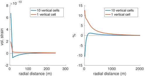
Figure 3: An example of a response function in 2D. Volumetric strain plotted as a function of distance from a central pressure perturbation. The left plot includes the value of perturbed grid cell itself. On the right plot, we have suppressed the perturbed grid cell and rescaled the curves to show percent-wise response magnitude compared with the central value. A vertical aquifer resolution of 10 cells was used to compute the blue curves, whereas the red curves were computed using a vertical aquifer resolution consisting of a single cell. With just one vertical cell, the bulging effect (c.f. Figure 4) is not properly captured.

Figure 4: Left: arching effect - local pressure perturbation pushes caprock upwards, causing surrounding aquifer region to stretch. Right: bulging effect - local pressure perturbation causes the region to expand into the surrounding aquifer, causing compression of the neighboring rock.

3 Results

In this section, we present a couple of cases where we compare the solutions obtained using the fully coupled model (full model) with those obtained using our proposed method using precomputed response functions (PR model) and using the standard one-way coupled approach based on the use of local pore volume compressibility coefficients (local model).

For the computations, we use the simulation framework provided by Matlab Reservoir Simulation Toolbox [24]. Fluid flow is modeled using a first order finite-volume upstream-weighted two-point flux approximation numerical scheme, whereas mechanics is modeled using a discretization based on first-order virtual elements [13] supplemented with approximate higher-order energies to avoid artifacts that have been shown to arise for high cell aspect ratios. The interested reader is referred to [31] or [20] for related discussion.

In the full model, flow and mechanics equations are solved simultaneously as a full linear system. For the local model, the computed values of $\bar{c}_{m}$ are used for pore volume compressibility coefficients. Although the code is not optimized for speed, the use of preconditioned iterative linear solvers (the conjugated gradient method with incomplete Cholesky factorization; the biconjugate gradients stabilized method with ILU factorization using threshold and pivoting) significantly helped improve performance for all three models.

3.1 Simple 2D example

We begin by studying a very simple 2D injection example where fluid is injected into a 100 m thick aquifer at a depth of 1000 m. We consider pressure development for a constant bottom hole overpressure of 1 MPa over a period of 50 days, and compare the results calculated from our three models (full model, local model and PR model). We use constant stress for lateral boundary conditions. Other relevant simulation parameters are listed in Table 1. This particular example was chosen to illustrate the existence of two-way coupling effects in the near-well region.

Table 1: Parameter values for simple 2D example

Lateral extent	5 kilometers
Lateral resolution	31 cells
Vertical extent: overburden, aquifer, underburden	1000 m, 100 m, 800 m
Vertical resolution	10 cells, 5 cells, 10 cells
Young’s modulus, $\Omega_{aq},\Omega_{sd}$	1 GPa, 10 GPa
Poisson ratio, $\Omega$	0.3
Permeability, $\Omega_{aq}$	100 mD
Porosity, $\Omega_{aq}$	0.3
Fluid compressibility	$4\cdot 10^{-5}\text{bar}^{-1}$
Fluid viscosity	$0.8$ cP
Well bottom-hole overpressure	1 MPa
Duration of simulation	50 days
Timestep size	1 day

The cutoff threshold used to compute the truncated response functions $\tilde{\Psi}_{i}$ of the PR model is $10^{-2}$ times the maximum value of $\Psi_{i}$.

Aquifer pressure and corresponding pore volume changes for day 5 and day 50 are plotted in Figure 5 and 6. From the left plot of Figure 5, we see that the PR model reproduces quite well the result of the full model. In particular, we observe two zones with a local decrease in pressure, situated at either side of the injection well, which are fully captured by the PR model but not by the local model. These pressure drops are associated with the arching effect where an uplift of the caprock caused by high pressure around the well leads to stretching and expansion of the aquifer rock in a wider area. In our scenario, the full model and PR model are thus able to predict a brief inflow and accumulation of fluid into these regions at early times, an effect that cannot be captured by the local model.

The right plot of Figure 5 shows the fractional change in aquifer pore volume (current minus pre-injection) for day 5, i.e. the time-integrated first two terms of (14). For the full model, the volumetric strain $\epsilon$ is immediately available since we have access to the displacements at simulation time. For the PR model, $\epsilon$ is approximated using our precomputed response functions $\{\tilde{\Psi}_{i}\}_{i=1,...,M}$ with (32). For the local model, we use (24). In other words, we plot the pore volume changes as they are computed with regards to the accumulation term of the pressure equation, not in terms of the displacements that can be computed post-hoc from one-way coupling with mechanics system.

We note that the local model significantly overpredicts pore volume change closest to the well, and slightly underpredicts it for about a kilometer before reaching zero. At very early times, the overprediction close to the well means that the corresponding pressure is less than what is obtained with a two-way coupled model. When day 5 is reached, the increase in pore volume is still significantly overestimated. Nevertheless, the corresponding pressure is very close to the correct value. This is because the pore volume in itself does not matter for the accumulation term in (14), only its change over time, which is already considerably smaller than for the first couple of timesteps.

At 50 days (Figure 6), we see that the three models all produce practically similar pressure profiles, whereas a large discrepancy remains in terms of pore volumes. It is interesting to note that the local model, with its additional assumptions and computational simplicity, already after 50 days produce results that are virtually identical to those given by the two-way coupled models for this scenario.

Maximal and mean squared errors are presented in Table 2.

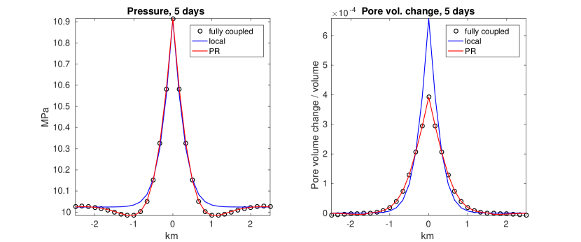
Figure 5: Pressure and pore volume change profiles at day 5 for the simple 2D injection example of this section

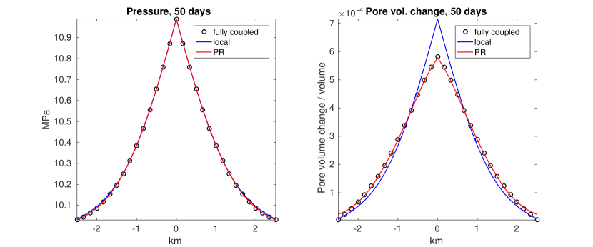
Figure 6: Pressure and pore volume change profiles at day 50 for the simple 2D injection example of this section

Table 2: Maximal and mean squared errors for simple 2D example, in percent of total aquifer pressure variation (0.93 MPa for day 5 and 0.96 MPa for day 50)

	Day 5		Day 50
Model	Max error	Mean sq. error	Max error	Mean sq error
Local	5.32	3.19	0.79	0.43
PR	0.29	0.15	0.23	0.15

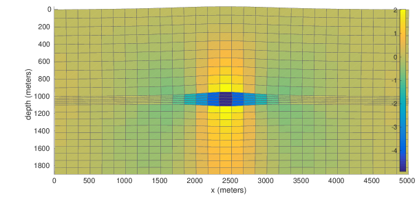
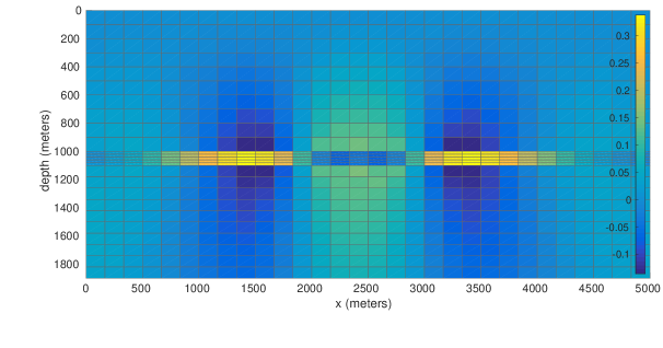
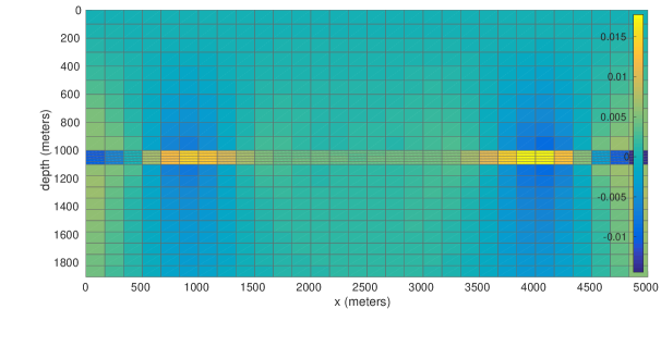
Figure 7: Change in vertical stress for aquifer, overburden and underburden at day 5 for the simple 2D injection example of this section. Contrary to the sign convention used in the linear elasticity formulation in the previous section, we here employ the convention more prevalent in geomechanics literature where a positive sign indicates compressive stress. Units are in bar. Top: Vertical stress change computed using the full model. Grid has been deformed to indicate the corresponding displacements (exaggerated). Middle: Error between vertical stress computed from the full model and the local model. Bottom: Error between vertical stress computed from the full model and the PR model.

Finally, we look at how discrepancies in pressure between the different models impact the mechanics part of the solution. As an example, we examine changes in vertical stress. The top plot in Figure 7 visualizes the change from initial state in vertical stress field at day 5 using the full model. The following two plots show the error between the vertical stress field produced by the full model and those produced by the local and PR models, respectively. We note that the maximum error of the local model is about twenty times higher than that of the PR model, for this timestep. From the bottom plot, we can see that the vertical stress field from the PR model closely matches that of the full model in the middle two kilometers or so. The largest error is located at a distance of about 1500 meters, which is related to the truncation of the response functions associated with cells closest to the injection well.

3.2 3D injection example

We will now apply and compare our three methods on a 3D injection example that borrows from the first benchmark problem in [15], whose details are largely based on previous injection operations at the In Salah Carbon Capture and Storage site [35]. We chose this example because of its relation to a real injection scenario where geomechanics issues have played an important role. However, for simplicity we restrict ourselves to one-phase flow.

For the flow simulation, we consider injection into a uniformly 20 m thick, horizontal aquifer. Our model covers 10 km of this aquifer in each lateral direction ($\Omega_{aq}$). The aquifer is located at a depth of 1800 m, with fixed pressure imposed at lateral boundaries and an impermeable top and bottom. In addition to the aquifer, the mechanical system includes the over- and underburden. The overburden consists of a “shallow” and a “deep” part with different elastic properties. The shallow part ($\Omega_{ob,s}$) extends from the surface down to a depth of 900 meters, whereas the deep part ($\Omega_{ob,d}$) consists of the zone from 900 m to the aquifer depth of 1800 m. The underburden ($\Omega_{ub}$) extends from the bottom aquifer boundary to a depth of 4000 m, where we impose a a zero displacement boundary condition. Lateral and top boundary conditions are of the fixed-stress type. At the beginning, we consider the aquifer and surrounding domain to be in mechanical and hydrostatic equilibrium. Further specifics on simulation grid and parameters used are given in Table 3.

We simulate injection of fluid into the aquifer through a vertical well located at the horizontal center of the modeled domain. The well is perforated along the full vertical extent of the aquifer. In a first simulation case (CASE 1), we consider a long-term, constant-rate injection for a total duration of 3 years (1 month timesteps). The volumetric injection rate is set to 0.02 m³/s at aquifer conditions, which has been chosen to approximate the volumetric injection rate of CO₂ considered in [35], taking the inherent density differences between the injected fluids (water vs. CO₂) at aquifer conditions into account. In a second simulation case (CASE 2), we consider a staggered injection pattern where 10 days of injection are followed by 10 days of shut-off before the cycle is repeated, for a total simulated period of 90 days (5 day timesteps).

Table 3: Parameter values for 3D injection example

Lateral extent	10 x 10 kilometers
Lateral resolution	21 x 21 cells
Layer thicknesses $\Omega_{ob,s}$, $\Omega_{ob,d}$, $\Omega_{aq}$, $\Omega_{ub}$	900 m, 900 m, 20 m, 2180 m
Vertical resolution $\Omega_{ob,s}$, $\Omega_{ob,d}$, $\Omega_{aq}$, $\Omega_{ub}$	3 cells, 4 cells, 3 cells, 7 cells
Young’s modulus $\Omega_{ob,s}$, $\Omega_{ob,d}$, $\Omega_{aq}$, $\Omega_{ub}$	1.5 GPa, 20 GPa, 6 GPa, 20 GPa
Poisson ratio $\Omega_{ob,s}$, $\Omega_{ob,d}$, $\Omega_{aq}$, $\Omega_{ub}$	0.2, 0.15, 0.2, 0.15
Aquifer porosity $\Omega_{ob,s}$, $\Omega_{ob,d}$, $\Omega_{aq}$, $\Omega_{ub}$	0.1, 0.01, 0.17, 0.15
Aquifer permeability	13 mD
Fluid compressibility	$4\cdot 10^{-5}\text{bar}^{-1}$
Fluid viscosity	$0.32$ cP
Fluid density	1000 kg/m3
Rock density	3000 kg/m3
Biot-Willis coefficient $\alpha$	1

The cutoff threshold for truncating the response functions $\tilde{\Psi}_{i}$ of the PR model was set to 10^-3 of the $\Psi_{i}$ maximum value.

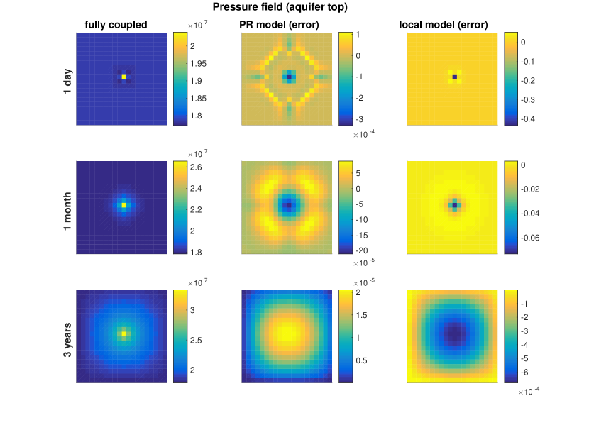
Figure 8: Top view of aquifer pressure at caprock level, for the continuous injection scenario (CASE 1). Rows represent the status at one day, one month and three years after injection start, respectively. The first column presents the pressure solution computed by the full (two-way coupled) model, with units in Pascal. The second column shows the discrepancy between the full and the PR model, and the third column the discrepancy between the full and the local model, measured as fraction of total pressure change in aquifer (unitless).

On Figure 8 we compare the outcomes of our three different simulation approaches in terms of the computed aquifer pressure field at selected points in time after injection start for CASE 1. From the top row we can see that after the first day, the local model underestimates the pressure in the central grid cell by about 40%, whereas the maximum error introduced by the PR model is on the order of 10^-4, measured as a fraction of maximum overpressure. After 1 month, the error in the local model has shrunk to 6%, whereas the error using the PR model remains around 10^-4. At 3 years (end of simulation), the local model and PR model both produce results that are very close to the fully coupled solution.

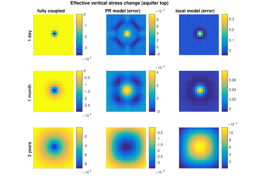
Figure 9: Top view of change in effective vertical stress in aquifer at caprock level, for the continuous injection scenario (CASE 1). Rows represent the status at one day, one month and three years after injection start, respectively. On the figure, a positive sign indicates compressive stress. The first column presents the effective vertical stress computed by the full (two-way coupled) model, with units in Pascal. The second column shows the discrepancy between the full and the PR model, and the third column the discrepancy between the full and the local model, measured as fraction of total vertical stress change in aquifer (unitless).

A similar trend can be seen in Figure 9, where we present the corresponding changes in effective normal stress at the top of the aquifer for CASE 1. Again, we see that for all timesteps, the error made by the PR model remains on the order of 10^-4 or less of total stress change, whereas the error resulting from the local model progressively shrinks from about 30% after day one to 6% after a month and 10^-3 at the end of simulation.

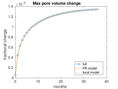
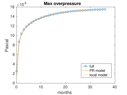
Figure 10: Temporal development of maximum pore volume change and maximum overpressure in aquifer for the continuous injection scenario (CASE 1). Maximum pore volume change expressed as fraction of bulk volume.

On figure 10, we track maximum change in pore volume and maximum overpressure measured in the aquifer over time for CASE 1. We see that the three approaches produce curves that are very close, and only for the first few timesteps is it possible to see any appreciable difference. From all plots presented so far for CASE 1, it seems clear that the PR model produce consistent, good results, but that the local model also produce good results except for the very early period after injection start.

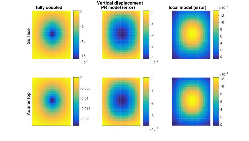
Figure 11: Vertical uplift at end of simulation period for the continuous injection scenario (CASE 1). Upper row represents surface level and lower row aquifer caprock level. The first column presents the vertical uplift computed by the full (two-way coupled) model, with units in meters. The second column shows the discrepancy between the full and the PR model, and the third column the discrepancy between the full and the local model, measured as fraction of maximum uplift (unitless).

Vertical uplift around the injection area is a feature of the In Salah injection operation that has been extensively studied and presented in past literature. For our CASE 1, the simulated uplift after 3 years is presented in Figure 11. Regardless of approach, we arrive at a maximum surface uplift of about 1.5 cm (z-axis oriented downwards). This is consistent with the range of values arrived at in [35] which is also based on a coupled flow and geomechanics model. However, it should be noted that our example is limited to one-phase flow and thus not directly comparable.

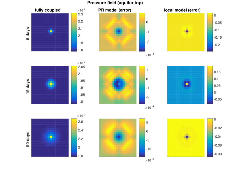
Figure 12: Top view of aquifer pressure at caprock level, for the staggered injection scenario (CASE 2). Rows represent the status at one day, one month and three years after injection start, respectively. The first column presents the pressure solution computed by the full (two-way coupled) model, with units in Pascal. The second column shows the discrepancy between the full and the PR model, and the third column the discrepancy between the full and the local model, measured as fraction of total pressure change in aquifer (unitless).

We now look at the corresponding results for CASE 2, which is a shorter-term scenario with a non-uniform injection rate that prevents the system from converging towards a long-term steady state. As such, we expect a priori that the impact of using a fully-coupled model will be stronger. The total period modeled is 90 days. Using a timestep duration of 5 days, the well switches between on and off status each second timestep.

On Figure 12, we plot aquifer pressure at 5 days, 15 days and 90 days for CASE 2. Similar to CASE 1, the discrepancy introduced by using the PR model remains at the order of 10^-4 of maximum overpressure for all three timesteps. On the other hand, the local model error has a maximum error of about 20% after five days, and the error remains at 8% at the end of simulation. The error is largely confined to the first few kilomters around the well. Similar observations regarding the overall error behavior from the PR and local models can be made looking at the vertical stress change plots in Figure 13, although the error in the local model is here less strongly concentrated around the well.

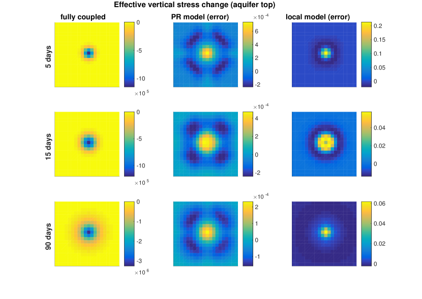
Figure 13: Top view of effective vertical stress in aquifer at caprock level, for the staggered injection scenario (CASE 2). Rows represent the status at one day, one month and three years after injection start, respectively. On the figure, a positive sign indicates compressive stress. The first column presents the effective vertical stress computed by the full (two-way coupled) model, with units in Pascal. The second column shows the discrepancy between the full and the PR model, and the third column the discrepancy between the full and the local model, measured as fraction of total vertical stress change in aquifer (unitless).

From the CASE 2 temporal plots of maximum pore volume change and overpressure in Figure 14, we note that the curves representing the outcomes from the full and PR models remain close together, whereas the curves representing the local model are noticeably different. Qualitatively, we observe that the variations both in pore volume and pressure obtained from the local model are weaker than those obtained from the other two models, which take two-way coupling into account. However, it should be noted that grid resolution seems to have some impact on the magnitude of this discrepancy. Figure 15 present the corresponding curves after re-running our simulations on a grid with about three times higher lateral resolution (61 x 61). As we can see, the difference between the local model and the full and PR model is now considerably smaller.

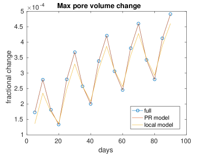
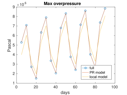
Figure 14: Temporal development of maximum pore volume change and maximum overpressure in aquifer for the staggered injection scenario (CASE 2). Maximum pore volume change expressed as fraction of bulk volume.

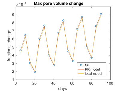
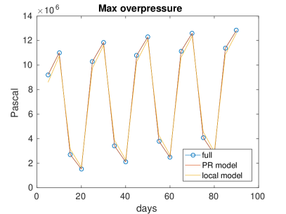
Figure 15: Temporal development of maximum pore volume change and maximum overpressure in aquifer for the staggered injection scenario (CASE 2), as simulated using a grid model with three times higher lateral resolution than in Figure 14. Maximum pore volume change expressed as fraction of bulk volume.

Table 4: Computational runtimes (seconds) for simulating CASE 1 and CASE 2 using the full, PR and local model

Model	Case	Flow	Mechanics	Total	Timesteps
Full	1	-	-	683.0	37
PR	1	8.8	85.0	93.8	37
Local	1	4.4	84.6	89.0	37
Full	2	-	-	382.7	18
PR	2	6.0	38.7	44.7	18
Local	2	2.7	46.7	49.4	18

The computational time for running CASE 1 and CASE 2 are presented in Table 4. The simulations were run on a standard workstation equipped with a six-core Intel Core i7-3930K CPU and 20 GB RAM. For the PR and local models, runtime is broken down into “Flow” (time to run the flow simulation) and “Mechanics” (time spent in post-hoc computation of displacements, strains and stresses). It is important to keep in mind the prototype nature of the simulation software used. Neither model has been optimized with regards to speed. For instance, very conservative tolerances were used for the fixed-stress split solver used to compute the fully coupled solution, resulting in a number of linear and nonlinear iterations that might be higher than necessary. Nevertheless, the figures in the table suggest that solving the system using the PR model represents an important gain in efficiency compared with the full model, and remains computationally comparable with the local model. In our test cases, the computing time required for solving the flow equation using the PR model was about twice the time spent using the local model. The difference is caused by a larger number of nonzeros in the linear system to solve, as further discussed below.

Prior to running the simulations, the response functions had to be computed as a preprocessing step. This calculation took 147 seconds for our grid. The response functions can be reused for any simulation on this grid as long as elastic moduli or mechanical boundary conditions do not change.

3.3 Practical computational issues

The precomputation of response functions, which happen once and can be associated with the initial grid generation step, does incur significant computational cost. In theory, each response function $\Psi_{i}$ requires solving the linear system consisting of the discretized force balance equations (7) for a given right-hand side that represents the impulse $\phi_{i}$. For large aquifer models, the number of response functions can be very high (one per aquifer cell or one per vertical column of aquifer cells). There are however some ways to mitigate this cost.

First, the linear system to solve, as represented by matrix M in (22), is symmetric, and can be efficiently solved using a preconditioned iterative solver for symmetric systems. Our experience is that the conjugated gradient algorithm preconditioned with incomplete Cholesky factorization works well in practice.

Second, the task of computing response functions is trivial to parallelize. All computations work on the same immutable data and are completely independent of each other. The task of computing the full set of response functions can therefore be spread out across as many computational cores as is available, whether one is working on a standard modern multi-core laptop or using a high performance computing cluster. In contrast, the computational efforts required for solving a fully-coupled system using iterative techniques cannot be similarly parallelized.

Third, due to our use of thresholding, each truncated response function has limited support. Moreover, we know exactly what its rescaling factor is, namely $\bar{c}_{m}$. This allows us to compute several response functions at a time for each single solution of the linear system, as long as they are sufficiently spatially separated that their overlaps are practically negligible.

All three strategies above were used in combination when computing the response functions used in the numerical examples presented in this article.

It should be emphasized that thresholding has another important computational aspect. As the threshold is tightened, the support of each $\Psi_{i}$ widens, leading to more coefficients to store but also a larger number of nonzeros in the system matrix of the flow equation, i.e. the sparse approximation of the matrix $\textbf{E}+\textbf{S}+\Delta t\textbf{P}$ in (23). As the number of nonzeros of this matrix increases, iterative linear solvers will generally require more computing time to solve the associated linear system. The threshold should therefore not be set too low. In our experience, setting threshold to 10^-3 appeared to be a good compromise for the examples presented above.

4 Conclusions

Investigation of issues related to geological storage of CO₂ will in many cases require the ability to run a large number of numerical simulations within a reasonable amount of time. This necessitates the development of computationally lightweight models. The approach proposed in this paper, the use of precomputed response functions, is an attempt to extend the current range of simplified modeling capabilities for CO₂ storage [38, 28] to situations where full coupling between fluid flow and rock mechanics is desired.

The work we have presented here suggests that this approach can reproduce, to a good degree of approximation, the results from a fully-coupled fluid flow and geomechanics simulation within the framework of linear poroelasticity, while remaining comparable to a traditional flow simulation in terms of computational requirements. The work required for adapting traditional reservoir simulator software to our approach amounts to simple modification of the accumulation term in the mass conservation equation(s), so that the pore volume of a given grid cell depends not only on pressure within that cell, but also on neighboring pressures within a certain distance. This can be seen as a generalization of the common use of pore volume compressibility coefficients.

On the other hand, the approach where a traditional flow simulation is one-way coupled with a mechanics solver seems to perform very well in many situations, Moreover, the use of an numerically computed $\bar{c}_{m}$ does allow to account to a certain extent for material heterogeneities and different boundary conditions, and the corresponding local model can indeed be seen as a limit case of our proposed approach based on precomputed responses.

In our experience the need for full coupling thus appears to be most relevant for models of limited spatial extent, short-term temporal scale, or to cases that involve significant temporal variation. As we saw for the 3D example above, the use of varying injection rates leads to a system that does not rapidly approach quasi-steady state conditions, and thus the non-local geomechanical impact on flow persists over time. Regarding this point, it is worth to mention that real-life injection operations will amost always suffer from transiently varying injection, whether it be for regular maintenance, or by design, as is the case of offshore injection by ship.

It is also possible that more complex simulation models than those examined herein will exhibit stronger coupling behavior, e.g. when using strain-dependent permeability. Whenever this coupling is strong enough to justify the extra computational and algorithmic overhead, the use of precomputed response functions can allow this coupling to be accounted for within the flow simulator itself in a computationally efficient way.

In the context of CO₂ storage, geomechanical studies are often associated with the need to understand the risk posed by nearby faults, whose mechanical behavior might not be properly described within a linear poroelastic framework. In that case, a hybrid model can be envisaged where the aquifer and rock matrix away from the fault is described using the linear theory, whereas the fault itself is modeled using nonlinear constitutive relationships. In such situations, precomputed response functions might still be used to describe the mechanical behavior of the part of the aquifer system that behaves linearly, away from the fault itself. However, this has not yet been tried and remains a topic for future research.

We conclude that the use of precomputed response functions offers the possibility to include the full impact of two-way geomechanical coupling into a stand-alone flow simulation in a computationally efficient way. The method appears to work well and to offer significant advantages, in particular for cases where many simulations need to be carried out. Further demonstration of the practical utility of the method will however require clear use cases that are both relevant for CO₂ storage and not already sufficiently well described by the considerably simpler local approach based on pore volume compressibility coefficients, in particular when combined with the use of $\bar{c}_{m}$.

5 Acknowledgments

This work was funded by the MatMoRa-II project, Contract no. 21564, sponsored by the Research Council of Norway and Statoil ASA.

6 Appendix

6.1 Analytical solution of the force equilibrium equation on an unbounded domain

This argument is adapted from the discussion at the beginning of Chapter 5 of [41]. We consider the poroelastic force equilibrium equation on an unbounded 3D domain:

$$\nabla\cdot(G\nabla\textbf{u})+\nabla\left((K+\frac{1}{3}G)\nabla\cdot\textbf{u}\right)=\alpha\nabla p-\textbf{F}\;\;\text{in}\;\;\Omega=\mathbb{R}^{3}$$ (33)

where F represent some body force. Using $c_{m}=\frac{\alpha}{K_{v}}$ along with standard relations between poroelastic parameters, it can be readily verified that a particular solution to (33) is given by:

$$u_{i}=\frac{\partial\Phi}{\partial x_{i}}$$ (34)

if $\Phi$ is some scalar potential that satisfies:

$$\nabla^{2}\Phi=c_{m}p$$ (35)

However, the Laplacian of $\Phi$ is then the volumetric strain, since:

$$\nabla^{2}\Phi=\frac{\partial u_{k}}{\partial x_{k}}=\epsilon_{kk}=\epsilon$$ (36)

Thus, the solution obtained implies that $\epsilon=c_{m}p$. In other words, volumetric strain at any given point is directly proportional to the pressure at that point, and consequently the relation between volumetric strain and pressure is purely local, assuming an unbounded domain and constant values of $K,G$ and $\alpha$.

6.2 Demonstration that $\int_{\Omega_{aq}}\Psi_{i}dx=\bar{c}_{m}$ on a discrete grid

We depart from expression (32). We assume that $\Psi_{i}$ represents the volumetric strain response to a unit pressure increase in cell $i$ (i.e. the impulse function $\phi_{i}$ equals 1 on cell $i$ and zero elsewhere). We further consider that $\tilde{\epsilon}$ and $\Psi_{i}$ are cell-wise constant, in which case we write $\tilde{\epsilon}_{j}$ and $\Psi_{i,j}$ to represent their values on grid cell $j$. (32) can then be written:

$$\tilde{\epsilon}_{j}=\sum_{i=1}^{M}\tilde{p}_{i}\Psi_{i,j}$$ (37)

As we have previously specified $\bar{c}_{m,j}$ to represent the local volumetric strain response in cell $j$ for a aquifer-wide unit pressure increase, we obtain:

$$\bar{c}_{m,j}=\sum_{i=1}^{M}\Psi_{i,j}$$ (38)

However, from its definition, $\Psi_{i,j}$ is also element $(i,j)$ of matrix E in (23), which is symmetric. Hence:

$$\bar{c}_{m,j}=\sum_{i=1}^{M}\Psi_{i,j}=\sum_{i=1}^{M}\Psi_{j,i}=\int_{\Omega_{aq}}\Psi_{j}dx$$

In other words, the total volumetric strain across the aquifer resulting from a pressure increase in cell $j$ also equals $c_{m,j}$. When $c_{m}$ is used as a pore volume compressibility coefficient in a decoupled flow simulation, this is equivalent to considering that all volumetric strain caused by a pressure increase in a cell $i$ is concentrated to that cell.

We now present an informal argument to suggest a similar result in the continuous case. We start by considering (33) on the form:

$$\mathcal{L}(\tilde{\textbf{u}})=\alpha\nabla\tilde{p}$$ (39)

where $\mathcal{L}$ is the linear, self-adjoint differential operator associated with the left hand side of (33) with specified boundary conditions, and we ignore the body force F since we are only concerned with changes in u (which we denote $\tilde{\textbf{u}}$), with respect to changes in $p$ (which we denote $\tilde{p}$). If we assume that the zero-displacement (Dirichlet) part of the boundary has nonzero measure, Korn’s inequality assures a trivial kernel of $\mathcal{L}$. The associated Green’s function $G(x,\xi)$ satisfies:

$$\mathcal{L}G(x,\xi)=\delta(x-\xi)$$ (40)

where $\delta$ denotes the delta function. $G(x,\xi)$ is a rank two tensor that expresses the displacement vector at $u$ caused by a force applied at $\xi$. Since $\mathcal{L}$ is self-adjoint, $G$ is symmetric, i.e. $G(x,\xi)=G(\xi,x)$. This also immediately follows from Maxwell’s reciprocity relation.

The displacement $\tilde{u}$ caused by a pressure variation $\tilde{p}$ in the domain can be written:

$$\tilde{u}(x)=\int_{\Omega}G(x,\xi)\nabla\tilde{p}(\xi)d\xi=-\int_{\Omega}\nabla_{\xi}\cdot G(x,\xi)\tilde{p}(\xi)d\xi$$ (41)

We have here loaded the differential operator $\nabla$ onto $G$ in the $\xi$ argument. For a unit pressure increase across $\Omega$, we thus have:

$$\tilde{u}(x)=-\int_{\Omega}\nabla_{\xi}\cdot G(x,\xi)d\xi$$ (42)

Using the symmetry of $G$, the divergence of $\tilde{u}$ at $x$ for a unit pressure increase across $\Omega$ can be developed as follows:

$$\nabla\cdot\tilde{u}(x) =\int_{\Omega}\nabla\cdot u(s)\delta(s-x)ds$$

$$=-\int_{\Omega}\nabla_{s}\cdot\left(\int_{\Omega}\nabla_{\xi}\cdot G(s,\xi)d\xi\right)\delta(s-x)ds$$

$$=-\int_{\Omega}\nabla_{\xi}\cdot\left(\int_{\Omega}\nabla_{s}\cdot G(\xi,s)\delta(s-x)ds\right)d\xi$$ (43)

Comparing with (41), the expression inside the parentheses on the last line of (6.2) expresses the displacement at $\xi$ resulting from a delta pressure at $x$. The full expression of the last line thus represent the integrated divergence of displacement (volumetric strain) across $\Omega$ associated with a delta pressure at $x$.

Thus the volumetric strain at $x$ resulting from unit pressure increase across $\Omega$ equals the integrated volumetric strain across $\Omega$ resulting from a delta pressure in $x$.

References

- [1] O. Andersen, S.E. Gasda, and H.M. Nilsen. Vertically averaged equations with variable density for CO2 flow in porous media. Transp. Porous Media, pages 1–33, 2014.
- [2] CM Aruffo, A Rodriguez-Herrera, E Tenthorey, F Krzikalla, J Minton, and A Henk. Geomechanical modelling to assess fault integrity at the co2crc otway project, australia. Australian Journal of Earth Sciences, 61(7):987–1001, 2014.
- [3] Maurice A. Biot. General theory of three-dimensional consolidation. Journal of Applied Physics, 12(2):155–164, 1941.
- [4] RC Bissell, DW Vasco, M Atbi, M Hamdani, M Okwelegbe, and MH Goldwater. A full field simulation of the in salah gas production and co 2 storage project using a coupled geo-mechanical and thermal fluid flow simulator. Energy Procedia, 4:3290–3297, 2011.
- [5] Tore I. Bjørnarå, Jan M. Nordbotten, and Joonsang Park. Vertically integrated models for coupled two-phase flow and geomechanics in porous media. Water Resources Research, 52(2):1398–1417, 2016.
- [6] Frédéric Cappa and Jonny Rutqvist. Seismic rupture and ground accelerations induced by co2 injection in the shallow crust. Geophysical Journal International, 190(3):1784–1789, 2012.
- [7] Frédéric Cappa and Jonny Rutqvist. Impact of co2 geological sequestration on the nucleation of earthquakes. Geophysical Research Letters, 38(17), 2011.
- [8] M. A. Celia, S. Bachu, J. M. Nordbotten, and K. W. Bandilla. Status of CO2 storage in deep saline aquifers with emphasis on modeling approaches and practical simulations. Water Resources Research, 51(9), 2015.
- [9] Melanie Yvonne Darcis. Coupling models of different complexity for the simulation of co2 storage indeep saline aquifers. 2013.
- [10] JP Davies, DK Davies, et al. Stress-dependent permeability: characterization and modeling. In SPE Annual Technical Conference and Exhibition. Society of Petroleum Engineers, 1999.
- [11] Rick H Dean, Xiuli Gai, Charles M Stone, Susan E Minkoff, et al. A comparison of techniques for coupling porous flow and geomechanics. Spe Journal, 11(01):132–140, 2006.
- [12] Ola Eiken, Philip Ringrose, Christian Hermanrud, Bamshad Nazarian, Tore A. Torp, and Lars Høier. Lessons learned from 14 years of CCS operations: Sleipner, In Salah and Snøhvit. Energy Procedia, 4:5541–5548, 2011. 10th International Conference on Greenhouse Gas Control Technologies.
- [13] Arun L Gain, Cameron Talischi, and Glaucio H Paulino. On the virtual element method for three-dimensional linear elasticity problems on arbitrary polyhedral meshes. Computer Methods in Applied Mechanics and Engineering, 282:132–160, 2014.
- [14] Giuseppe Gambolati, R. W. Lewis, B. A. Schrefler, and L. Simoni. Comment on ’coupling versus uncoupling in soil consolidation’. International Journal for Numerical and Analytical Methods in Geomechanics, 16(11):833–837, 1992.
- [15] S. Gasda, M. Darcis, M. White, B. Flemish, and H. Class. Geomechanical behavior ofCO2 storage in saline aquifers (geocosa): benchmark problem description, 2013.
- [16] S. E. Gasda, J. M. Nordbotten, and M. A. Celia. Vertically averaged approaches for CO2 migration with solubility trapping. Water Resources Research, 47(5), 2011.
- [17] Sarah E. Gasda, Halvor M. Nilsen, and Helge K. Dahle. Impact of structural heterogeneity on upscaled models for large-scale CO2 migration and trapping in saline aquifers. Advances in Water Resources, 2013.
- [18] V Girault, Kundan Kumar, and Mary F Wheeler. Convergence of iterative coupling of geomechanics with flow in a fractured poroelastic medium. Technical report, Technical Report ICES REPORT 15-05, The Institute for Computational Engineering and Sciences The University of Texas at Austin, Austin, Texas 78712, 2015.
- [19] Jihoon Kim. Sequential methods for coupled geomechanics and multiphase flow. PhD thesis, Stanford University, 2010.
- [20] Øystein Strengehagen Klemetsdal. The virtual element method as a common framework for finite element and finite difference methods. Master’s thesis, Norwegian University of Science and Technology, 2016.
- [21] RW Lewis, BA Schrefler, and L Simoni. Coupling versus uncoupling in soil consolidation. International Journal for Numerical and Analytical Methods in Geomechanics, 15(8):533–548, 1991.
- [22] P Longuemare, M Mainguy, P Lemonnier, A Onaisi, Ch Gérard, and N Koutsabeloulis. Geomechanics in reservoir simulation: overview of coupling methods and field case study. Oil & Gas Science and Technology, 57(5):471–483, 2002.
- [23] Andro Mikelić and Mary F Wheeler. Convergence of iterative coupling for coupled flow and geomechanics. Computational Geosciences, 17(3):455–461, 2013.
- [24] MRST. The MATLAB Reservoir Simulation Toolbox. \hrefhttp://www.sintef.no/MRST/www.sintef.no/MRST, 12 2015b.
- [25] Halvor Møll Nilsen, Knut-Andreas Lie, and Odd Andersen. Analysis of CO2 trapping capacities and long-term migration for geological formations in the Norwegian North Sea using MRST-co2lab. Computers & Geoscience, 79:15–26, 2015.
- [26] Halvor Møll Nilsen, Knut-Andreas Lie, and Odd Andersen. Fully implicit simulation of vertical-equilibrium models with hysteresis and capillary fringe. Comput. Geosci., :, 2015.
- [27] J. M. Nordbotten and H. K. Dahle. Impact of the capillary fringe in vertically integrated models for CO2 storage. Water Resour. Res., 47(2):W02537, 2011.
- [28] Jan M. Nordbotten and Michael A. Celia. Geological Storage of CO2: Modeling Approaches for Large-Scale Simulation. John Wiley & Sons, Hoboken, New Jersey, 2012.
- [29] Amélie Ouellet, Thomas Bérard, Jean Desroches, Peter Frykman, Peter Welsh, James Minton, Yusuf Pamukcu, Suzanne Hurter, and Cornelia Schmidt-Hattenberger. Reservoir geomechanics for assessing containment in co 2 storage: a case study at ketzin, germany. Energy Procedia, 4:3298–3305, 2011.
- [30] Matthias Preisig and Jean H Prévost. Coupled multi-phase thermo-poromechanical effects. case study: Co 2 injection at in salah, algeria. International Journal of Greenhouse Gas Control, 5(4):1055–1064, 2011.
- [31] Xavier Raynaud, Stein Krogstad, and Halvor Møll Nilsen. On the use of the virtual element method for geomechanics on reservoir grids. In ECMOR XV – 15th European Conference on the Mathematics of Oil Recovery, Amsterdam, Netherlands, 29 August - 1 September 2016. EAGE, 2014.
- [32] J Rutqvist, J Birkholzer, F Cappa, and C-F Tsang. Estimating maximum sustainable injection pressure during geological sequestration of co 2 using coupled fluid flow and geomechanical fault-slip analysis. Energy Conversion and Management, 48(6):1798–1807, 2007.
- [33] Jonny Rutqvist. The geomechanics of co2 storage in deep sedimentary formations. Geotechnical and Geological Engineering, 30(3):525–551, 2012.
- [34] Jonny Rutqvist and Chin-Fu Tsang. A study of caprock hydromechanical changes associated with co2-injection into a brine formation. Environmental Geology, 42(2):296–305, 2002.
- [35] Jonny Rutqvist, Donald W Vasco, and Larry Myer. Coupled reservoir-geomechanical analysis of co 2 injection and ground deformations at in salah, algeria. International Journal of Greenhouse Gas Control, 4(2):225–230, 2010.
- [36] D.A. Settari, Antonin; Walters. Advances in coupled geomechanical and reservoir modeling with applications to reservoir compaction. SPE J., 6, 2001.
- [37] F.M. Settari, Antonin; Mourits. A coupled reservoir and geomechanical simulation system. SPE J., 3, 1998.
- [38] SINTEF ICT. The MATLAB Reservoir Simulation Toolbox: Numerical CO2 laboratory, October 2014.
- [39] Elena Tillner, Ji-Quan Shi, Giacomo Bacci, Carsten M Nielsen, Peter Frykman, Finn Dalhoff, and Thomas Kempka. Coupled dynamic flow and geomechanical simulations for an integrated assessment of co 2 storage impacts in a saline aquifer. Energy Procedia, 63:2879–2893, 2014.
- [40] James P Verdon, J-Michael Kendall, Anna L Stork, R Andy Chadwick, Don J White, and Rob C Bissell. Comparison of geomechanical deformation induced by megatonne-scale co2 storage at sleipner, weyburn, and in salah. Proceedings of the National Academy of Sciences, 110(30):E2762–E2771, 2013.
- [41] Herbert F Wang. Theory of linear poroelasticity. Princeton Series in Geophysics, Princeton University Press, Princeton, NJ, 2000.