The internal structure of overpressured, magnetized, relativistic jets

Abstract

This work presents the first characterization of the internal structure of overpressured steady superfast magnetosonic relativistic jets in connection with their dominant type of energy. To this aim, relativistic magnetohydrodynamic simulations of different jet models threaded by a helical magnetic field have been analyzed covering a wide region in the magnetosonic Mach number - specific internal energy plane. The merit of this plane is that models dominated by different types of energy (internal energy: hot jets; rest-mass energy: kinetically dominated jets; magnetic energy: Poynting-flux dominated jets) occupy well separated regions. The analyzed models also cover a wide range of magnetizations. Models dominated by the internal energy (i.e., hot models, or Poynting-flux dominated jets with magnetizations larger than but close to 1) have a rich internal structure characterized by a series of recollimation shocks and present the largest variations in the flow Lorentz factor (and internal energy density). Conversely, in kinetically dominated models there is not much internal nor magnetic energy to be converted into kinetic one and the jets are featureless, with small variations in the flow Lorentz factor. The presence of a significant toroidal magnetic field threading the jet produces large gradients in the transversal profile of the internal energy density. Poynting-flux dominated models with high magnetization ($\approx 10$ or larger) are prone to be unstable against magnetic pinch modes, which sets limits to the expected magnetization in parsec-scale AGN jets and/or constrains their magnetic field configuration.

1. Introduction

How relativistic jets are launched, accelerated, and collimated is probably one of the most important questions related to AGN jet physics and other astrophysical systems involving black hole accretion, such as $\gamma$-ray bursts (GRBs) or tidal disruption flares (TDFs). It is thought that dynamically important helical magnetic fields twisted by the differential rotation of the black hole’s accretion disk or ergosphere play an important role (Blandford & Znajek, 1977; Blandford & Payne, 1982; McKinney & Blandford, 2009; Tchekhovskoy, Narayan & McKinney, 2011; Zamaninasab et al., 2014). As the jet propagates, part of the magnetic energy of the plasma is converted into kinetic energy, accelerating the jet while maintaining a parabolic shape (see, e.g., Komissarov et al., 2007, and references therein for theoretical approaches to the problem; see Nakamura & Asada, 2013, for an investigation of the parabolic jet structure in M87). For initially relativistic hot jets, thermal acceleration can also play a role (see, e.g., Gómez et al., 1995, 1997). Simultaneous multi-wavelength and Very Long Baseline Interferometry (VLBI) observations of AGN jets suggest that the acceleration and collimation of the jet takes place in the innermost $10^{4-6}$ Schwarzschild radii from the central black hole, upstream of the millimeter VLBI (mm-VLBI) core (Marscher et al., 2008), defined as the bright compact feature in the upstream end of the observed VLBI jet.

The simultaneity of multi-wavelength flares (from radio to $\gamma$-ray energies) with the passage of a new superluminal component through the mm-VLBI core has led to the suggestion that this corresponds to a strong recollimation shock (e.g., Marscher et al., 2008, 2010; Casadio et al., 2015a, b). Moreover, in sources as CTA 102, in which this coincidence has not been proven, the presence of a stationary feature close to the VLBI core was claimed to explain the spectral evolution of a radio-flare (Fromm et al., 2011). Multifrequency VLBI observations showed evidence in this direction (Fromm et al., 2013a, b). The interaction of the moving shock associated with the superluminal component and the standing shock at or close to the mm-VLBI core would produce the particle acceleration and burst in particle and magnetic energy densities required to produce the multi-wavelength flares. It should be noted that this association of the mm-VLBI core with a recollimation shock would not be in contradiction with the predictions from the Blandford & Königl jet model (Blandford & Königl, 1979) that establishes the VLBI core as the location at which the jet becomes optically thin, as long as this transition at centimeter wavelengths takes place downstream of the mm-VLBI core.

Relativistic (magneto)hydrodynamical simulations have shown that pressure mismatches between the jet and ambient medium lead to the formation of a pattern of recollimation shocks (e.g., Wilson, 1987; Daly & Marscher, 1988; Dubal & Pantano, 1993; Gómez et al., 1995, 1997, 2016; Mimica et al., 2009; Porth & Komissarov, 2015; Mizuno et al., 2015). It is therefore natural to expect that if the mm-VLBI core corresponds to a recollimation shock other similar standing VLBI features would be observed downstream of its location. Indeed, although some stationary features have been found at hundreds of parsecs from the central engine (e.g., Roca-Sogorb et al., 2010), most of the stationary components observed in AGN jet appear in the innermost jet regions, close to the VLBI core (e.g., Jorstad et al., 2005; Cohen et al., 2014; Gómez et al., 2016). Hence, obtaining a better characterization of recollimation shocks is of special relevance not only for the interpretation of the observed VLBI structure in AGN jets, but also to obtain a better understanding of the nature of the mm-VLBI core and its connection with the emission mechanisms at X and $\gamma$-ray energies often observed from these sources.

Recollimation shocks have been previously studied through relativistic hydrodynamic and magnetohydrodynamic numerical simulations (e.g., Gómez et al., 1995, 1997; Komissarov & Falle, 1997; Matsumoto, Masada & Shibata, 2012; Porth & Komissarov, 2015; Komissarov, Porth & Lyutikov, 2015; Mizuno et al., 2015; Fromm et al., 2016). In this paper we present the first systematic study of the resulting jet structure in connection with the dominant type of energy in the jet, namely internal, kinetic, or magnetic, through relativistic magnetohydrodynamical simulations of overpressured superfast-magnetosonic jets propagating through a homogeneous ambient medium. The effect of a pressure-decreasing atmosphere in the structure of jets, particularly in the properties of recollimation shocks, and the jet energy conversion will be the subject of future research. The paper is organized as follows. In Section 2, we define the parameter space of our study. Axisymmetric jet models are injected into the two-dimensional numerical grid in transversal equilibrium to minimize radial perturbations. In Section 3 we describe the transversal structure of the injected models. Section 4 is devoted to describe the setup of the simulations, whereas in Section 5 we present and discuss the results on the internal structure of jets. Finally, in Section 6 we summarize our main conclusions.

2. Parameter space

In the purely hydrodynamical, Newtonian case, the basic parameters governing the propagation of a supersonic, initially cylindrical jet with purely axial speed across an homogeneous ambient medium at rest can be taken as (see, e.g., Norman et al., 1982) the jet density, $\rho_{j}$, the jet overpressure factor, $K$, and the internal jet Mach number, $M_{j}$. Models are expressed in units of the ambient medium density and pressure, $\rho_{a}$, $p_{a}$, and the jet radius at injection, $R_{j}$.

In the relativistic case, the presence of the light speed, $c$, as a constant appearing in the hydrodynamical equations, spawns an additional parameter and the simulations are defined by means of (see, e.g., Martí et al., 1997) $\rho_{j}$, $K$, the (axial) velocity of the flow in the jet, $v_{j}$, and the classical or relativistic internal jet Mach number, $M_{j}$, ${\cal M}_{j}$, respectively, in units of the ambient density and the jet radius at injection.

In the RMHD case, assuming that the radial magnetic field is zero at injection, two new quantities are needed to define the magnetic field configuration, namely the azimuthal and axial magnetic field components, $B^{\phi}_{j}$, $B^{z}_{j}$, or equivalently, the jet magnetization, $\beta_{j}$, and the magnetic pitch angle, $\phi_{j}$. The jet magnetization is defined as $\beta_{j}=p_{m,j}/p_{j}$, where $p_{m,j}$ and $p_{j}$ stand, respectively, for the jet magnetic pressure and the jet thermal (or gas) pressure. The magnetic pressure is defined as $p_{m,j}=b^{2}_{j}/2$, where $b^{2}_{j}$ is the magnetic energy density. On the other hand, in the case of supermagnetosonic jets as those considered here, the role of the Mach number will be played by the magnetosonic Mach number, ${\cal M}_{ms,j}$ (see the Appendix). Together with other parameters (significantly the jet overpressure factor, $K$), the relativistic magnetosonic Mach number governs the properties of internal conical shocks in overpressured magnetized jets in the same way as the Mach number does in purely hydrodynamic, overpressured jets. In this work, units are used in which the light speed, the ambient density and the jet radius at injection are set to unity. Besides that, a factor of $\sqrt{4\pi}$ is absorbed in the definition of the magnetic field. Finally, both the jet and the ambient medium plasmas are assumed to behave as a perfect gas with constant adiabatic index, $\gamma=4/3$. This value (which corresponds to the adiabatic index in the ultrarelativistic limit) is inappropriate to describe thermodynamically the plasma in the cold models. However, in these cases, the internal energy is negligible and to overestimate it by a factor of two with respect to the non-relativistic value obtained with an adiabatic index of $5/3$ has no qualitative effects on the jet dynamics. The adiabatic index of $4/3$ is also inadequate to describe the ambient medium but in these simulations where the ambient medium is static and fixed to its initial values, the effect of using one adiabatic index or another can be absorbed in the definition of plasma density.

Table 1Parameters defining the overpressured jet models.

Model	$\rho_{j}\,[\rho_{a}]$	$K$	$v_{j}\,[c]$	${\cal M}_{ms,j}$	$\beta_{j}$	$\phi_{j}$ [∘]	$\Delta r_{sl}^{a}\,[R_{j}]$	$\varepsilon_{j}\,[c^{2}]$	$K_{1}^{b}$	$p_{a}\,[\rho_{a}c^{2}]$
PH02	$5\times 10^{-3}$	$2$	$0.95$	$2.0\phantom{00}$	$2.77\phantom{0}$	$45.0$	0.12	10.00000	$1.87$	$3.31\times 10^{-2}$
PK02	$5\times 10^{-3}$	$2$	$0.95$	$2.0\phantom{00}$	$10.0\phantom{000}$	$45.0$	0.49	0.4580	$1.84$	$4.20\times 10^{-3}$
HP03	$5\times 10^{-3}$	$2$	$0.95$	$3.5\phantom{00}$	$0.454$	$45.0$	0.12	10.00000	$1.94$	$1.21\times 10^{-2}$
PK03	$5\times 10^{-3}$	$2$	$0.95$	$3.5\phantom{00}$	$10.0\phantom{000}$	$45.0$	0.49	0.1170	$1.84$	$1.08\times 10^{-3}$
KH06	$5\times 10^{-3}$	$2$	$0.95$	$6.0\phantom{00}$	$0.5\phantom{00}$	$45.0$	0.49	0.4680	$1.94$	$5.85\times 10^{-4}$
KP06	$5\times 10^{-3}$	$2$	$0.95$	$6.0\phantom{00}$	$10.0\phantom{000}$	$45.0$	0.32	0.0317	$1.84$	$2.90\times 10^{-4}$
KH10	$5\times 10^{-3}$	$2$	$0.95$	$10.0\phantom{00}$	$0.5\phantom{00}$	$45.0$	0.24	0.1330	$1.94$	$1.66\times 10^{-4}$
KP10	$5\times 10^{-3}$	$2$	$0.95$	$10.0\phantom{00}$	$10.0\phantom{000}$	$45.0$	0.24	0.0132	$1.84$	$1.21\times 10^{-4}$

^a $\Delta r_{sl}$ is the width of the shear layer defined as the radial section of the jet where the function defining the transition, sech$(r^{m})$, is between 0.1 and 0.9, corresponding to jet mass fractions between 0.1 and 0.9.
^b $K_{1}$ stands for the total (gas plus magnetic) overpressure factor at the jet surface (see text).

Table 1 displays the values of the six parameters (namely $\rho_{j}$, $v_{j}$, $K$, ${\cal M}_{ms,j}$, $\beta_{j}$ and $\phi_{j}$) defining the models. Given the type of transversal equilibrium profiles considered in this work (obtained for specific profiles of the azimuthal magnetic field as discussed in the next section), $K$, ${\cal M}_{ms,j}$, $\beta_{j}$ and $\phi_{j}$ represent jet cross section averages. All the jet models have the same rest-mass density and flow velocity, and the same average magnetic pitch angle and overpressure factor. On the contrary, the relativistic magnetosonic Mach number changes by a factor of 5 and the magnetization, by a factor of 20, among the different jet models. Note that all the models have initial toroidal speeds equal to zero and, consequently, are better suited to describe the jets at distances far beyond the jet formation region. Table 1 also displays some derived parameters, as the pressure mismatch at the jet surface, $K_{1}$, the ambient pressure, $p_{a}$, and the specific internal energy in the jet, $\varepsilon_{j}$. The ambient pressure changes more than two orders of magnitude, although its value is always small compared with the rest-mass energy density of the ambient medium. The values of the specific internal energy in the jet span three orders of magnitude including cold as well as hot jet models. Finally, the transition between the jet and the ambient medium is smoothed by means of a shear layer of width $\Delta r_{sl}$ by convolving the sharp jumps with the function sech$(r^{m})$, where $m\in[4,16]$. Different widths of the shear layer are needed to stabilize the models against pinch instabilities (see Sect. 5.2).

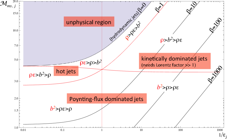
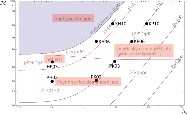
Figure 1.— Top panel: Jet classes in the ${\cal M}_{ms,j}-1/\varepsilon_{j}$ plane according to the dominant energy type, for given jet flow velocity, $v_{j}=0.95$. Drawn are lines of constant magnetization (0, 1, 10, 100, 1000). Kinetically dominated jets, Poynting flux dominated jets and hot jets are placed in the diagram with the help of three (red) lines corresponding to models with $\rho_{j}=\rho_{j}\varepsilon_{j}$, $b_{j}^{2}=\rho_{j}\varepsilon_{j}$, $b_{j}^{2}=\rho_{j}$. Pure hydrodynamic models are placed on the $\beta_{j}=0$ line which bounds a forbidden region (in violet) corresponding to unphysical models with negative magnetic energies. Bottom panel: Distribution on the ${\cal M}_{ms,j}-1/\varepsilon_{j}$ diagram of the models considered in this paper.

The parameters of the models are chosen to span a wide region in the ${\cal M}_{ms,j}$-$1/\varepsilon_{j}$ plane (see Fig. 1). According to the type of energy flux that dominates, jet models can be classified as kinetically dominated (those models dominated by the rest-mass energy, $\rho_{j}>\max(\rho_{j}\varepsilon_{j},b_{j}^{2})$ and Lorentz factor $W_{j}\gg 1$), internal energy dominated (or hot jets, $\rho_{j}\varepsilon_{j}>\max(\rho_{j},b_{j}^{2})$) and Poynting flux dominated ($b_{j}^{2}>\max(\rho_{j},\rho_{j}\varepsilon_{j})$). The plane displayed in Fig. 1 has the virtue of placing these three types of models in well separated regions. Our current understanding of the process of jet acceleration indicate that jets would form at some point in the hot/Poynting-flux dominated region and would evolve towards the region of kinematically dominated models (see, e.g., Komissarov et al., 2007, and references therein). When projected onto this diagram, the simulations discussed by Roca-Sogorb et al. (2008, 2009) would be placed on top of the line $1/\varepsilon_{j}=1$ with magnetizations $\beta_{j}\in[0.1,10]$, whereas those of Mizuno et al. (2015) will be on the line $1/\varepsilon_{j}=0.095$ with magnetizations $\beta_{j}\in[0,0.4]$. In all the cases, the models are in the hot models region or its neighbourhood.

Names are given to the models according to the following rule: two capital letters to indicate the two dominating energy types (“K”, for kinetically dominated jets; “P”, for Poynting-flux dominated jets; “H”, for hot jets) in order of prevalence, and two digits related with the Mach number of the jet flow.

3. Transversal structure of the injected jet models

Jets are injected in internal transversal equilibrium to minimize the sideways perturbations once immersed in the ambient medium and to obtain an internal structure as clean as possible. The profiles of the rest-mass density, the axial flow velocity and the axial magnetic field across the jet are taken constant.

The azimuthal magnetic field in the laboratory frame is defined according to

$$B^{\phi}(r)=\left\{\begin{array}[]{ll}\displaystyle{\frac{2B_{j,\rm m}^{\phi}(r/R_{B^{\phi},\rm m})}{1+(r/R_{B^{\phi},\rm m})^{2}}},&0\leq r\leq 1\\ 0,&r>1.\end{array}\right.$$ (1)

This function represents a toroidal magnetic field that grows linearly for $r\ll R_{B^{\phi},\rm m}$, reaches a maximum ($B_{j,\rm m}^{\phi}$) at $r=R_{B^{\phi},\rm m}$, then decreases as $1/r$ for $r\gg R_{B^{\phi},\rm m}$ and is set equal to zero for $r>1$. It is a smooth fit of the piecewise profile used by Lind et al. (1989) (see also Komissarov, 1999; Leismann et al., 2005) and corresponds to a uniform current density for radius $r\ll R_{B^{\phi},\rm m}$, declining up to $r=1$, and a return current at the jet surface. The radius at which the toroidal magnetic field reaches its maximum, $R_{B^{\phi},\rm m}$, has been fixed to 0.37 in all the models.

In the case of a jet without rotation, the equilibrium equation for the transversal equilibrium can be written (e.g., Martí, 2015)

$$\frac{dp}{dr}=-\frac{(B^{\phi})^{2}}{rW^{2}}-\frac{B^{\phi}}{W^{2}}\frac{dB^{\phi}}{dr},$$ (2)

where $p$ is the gas pressure and $W$, the jet Lorentz factor (corresponding in this case to a purely axial flow). This equation can be integrated by separation of variables to give

$$p(r)=\left\{\begin{array}[]{ll}\displaystyle{2\left(\frac{B_{j,\rm m}^{\phi}}{W(1+(r/R_{B^{\phi},\rm m})^{2})}\right)^{2}+C},&0\leq r\leq 1\\ p_{a}^{\prime},&r>1,\end{array}\right.$$ (3)

where we choose $p_{a}^{\prime}=Kp_{a}$ (with $K>1$) to obtain equilibrium models of overpressured jets. Using the boundary condition $p^{*}_{1}=p_{a}^{\prime}$, where $p^{*}$ is the total (gas plus magnetic) pressure and $p^{*}_{1}$ stands for $p^{*}(r\!=\!1)$, the integration constant $C$ can be fixed to be

$$C=p_{a}^{\prime}-\frac{(B_{j}^{z})^{2}}{2}-\frac{(B^{\phi}_{1})^{2}}{2W^{2}}(1+(R_{B^{\phi},\rm m})^{2}).$$ (4)

This transversal structure is convolved with a shear layer to smooth the transition between the jet and the ambient (see Sect. 2). It is interesting to note that by introduzing this shear layer, the current sheet at the jet surface is removed. Fig. 2 shows the (gas, magnetic and total) pressure profiles across the jets (including the shear layers) for the models considered in this paper. For our choice of parameters, the magnetic pressure

$$p_{m}(r)=\frac{{B_{j}^{\phi}(r)}^{2}}{W_{j}^{2}}+(B_{j}^{z})^{2},$$ (5)

is dominated by the (constant) contribution of the axial component of the magnetic field, although it is modulated by the profile of the toroidal component. Hence, it has a minimum at the jet axis, and then increases up to $r=R_{B^{\phi},\rm m}$ where it has the maximum. Beyond this point, the magnetic pressure decreases slowly with radius up to the surface.

Contrary to the magnetic pressure, the gas pressure has a local maximum at the jet axis and decreases progressively faster up to $r=R_{B^{\phi},\rm m}$. At larger radii, and before entering into the shear layer, the gas pressure tends to a constant value. Both thermal and magnetic pressure combine to produce the monotonically decreasing radial profile in the total pressure needed to balance the magnetic tension.

Although based on a particular choice of parameter profiles, the general conclusion is that the existence of a magnetic field with a significant toroidal component produces a complex transversal structure in magnetized jets with a central spine (extending up to the radius where the maximum of the magnetic tension is reached, some point between $r=0$ and $r=R_{B^{\phi},\rm m}$) where the thermal pressure (and hence the plasma internal energy) is close to its maximum. A layer with milder (magnetic, thermal) pressure profiles surrounds this central spine. This layer extends up to the outer jet/ambient-medium shear layer (see Fig. 2).

Finally, it can be easily seen that the presence of a toroidal field like the one defined in (1) increases the gas pressure up to $r=\sqrt{R_{B^{\phi},\rm m}((R_{B^{\phi},\rm m})^{2}-R_{B^{\phi},\rm m}+1)}$ ($\approx 0.53$, for $R_{B^{\phi},\rm m}=0.37$) and decreases it outside so that the average gas pressure inside the jet remains unchanged with respect to the case of zero toroidal magnetic field (Martí, 2015).

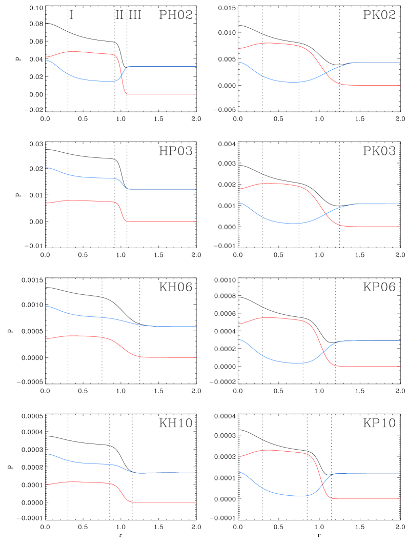
Figure 2.— Gas (blue filled line), magnetic (red filled line) and total pressure (black filled line) across the jet at injection for the eight models considered in this work. Models with the same magnetization (HP03, KH06 and KH10, on one side; PK02, PK03, KP06 and KP10 on the other) have the same pressure profiles (with slight variations due to the different widths of the shear layers). In models with magnetization smaller than $1.0$ (HP03, KH06, KH10), gas pressure dominates over magnetic pressure across the jet. Vertical dotted lines define the layers making up the transversal jet structure: $0<r<r_{\rm I}$: hot central spine; $r_{\rm II}<r<r_{\rm III}$: shear layer.

4. Numerical simulations

The numerical RMHD code used in these simulations is a second-order, conservative, finite-volume code based on high-resolution shock-capturing techniques. An overview of the specific algorithms used in the code and an analysis of its performance can be found in Appendices A and B, respectively, of Martí (2015).

The equilibrium profiles discussed in the previous section are used as a boundary condition to inject the jets into a two-dimensional domain representing an ambient medium with a pressure mismatch. In their attempt to reach again the equilibrium, the jets undergo sideways motions generating radial components of the flow velocity and the magnetic field that break the slab symmetry of the original jet model along the $z$-axis.

The jets are injected through a nozzle of radius $R_{j}$ equal to 1 into an axisymmetric cylindrical domain with $(r,z)\in[0,L_{r}]\times[0,L_{z}]$, with $L_{r}=6$ and $L_{z}=60,80,120$, depending on the spacing of the shocks in each model. The evolution of the flow in the domain is simulated with the RMHD code in 2D radial, axial cylindrical coordinates with a resolution of 80 (40) cells per jet radius in the radial (axial) direction. In order to disturb the ambient medium as little as possible along the simulation, the domain $(r,z)\in[0,1]\times[0,L_{z}]$ is initially filled with the analytical, injection solution. Reflecting boundary conditions are set along the axis ($r=0$, $z>0$) and at the jet base outside the injection nozzle ($r>1$, $z=0$). Zero gradient conditions are set in the remaining boundaries.

The models, set up to be in equilibrium with an ambient pressure $p^{\prime}_{a}=Kp_{a}$ ($K>1$), are injected into an atmosphere with pressure $p_{a}$. The new equilibrium states are set through a series of conical fast-magnetosonic shocks which are the subject of study of the present paper. Reaching such an equilibrium state is a lengthy process that typically takes between 3 and 5 axial grid light crossing times ($2-6\times 10^{4}$ time iterations) per simulation. In computational time this means about 10 to 50 days of single-processor CPU time. This time was reduced in practice by a factor of 10 using an OpenMP parallel version of the code with 12 processors. During this transient phase the flow suffers (more or less violent) axially-symmetric sideways expansions and compressions which in some cases had to be damped out with the help of the shear layer to avoid the growth of pinch instabilities (see Sect. 5.2).

5. Results

5.1. Overall jet structure

The steady state jets corresponding to the models defined in Table 1 are shown in Figs. 3 to 10. Each figure contains panels displaying the distributions of rest-mass energy density and gas pressure (both in logarithmic scale), flow Lorentz factor (with the poloidal streamlines overimposed), and toroidal and axial magnetic field components (with the poloidal magnetic field lines overimposed on the axial magnetic field panel). Besides these maps another one displaying the toroidal flow speed generated during the jet evolution is also shown. Small radial components of the flow speed and the magnetic field are also generated during the flow evolution but are not shown, although their magnitude relative to that of the corresponding axial component can be inferred from the bending of the poloidal lines. Some general conclusions can be extracted from the analysis of these figures:

1. In all the models, the equilibrium of the jet is established by a series of expansions and compressions of the jet flow against the ambient medium. Standing oblique shocks (recollimation shocks) associated with these jet oscillations can be distinguished in some cases, specially in hot models (PH02, HP03) and, to a lesser extent, in colder, low magnetization models (KH06, KH10). A more quantitative analysis of the jet oscillations and the standing shocks is presented in Sects. 5.2 and 5.3, respectively.

2. As a consequence of the profile of the magnetic pressure across the jet and, specially, of the magnetic pinch exerted by the toroidal magnetic field, the thermal pressure is not constant across the jet (see Fig. 2 and the accompanying discussion on the transversal structure of the injected jet models in Sect. 3). Models with large magnetizations (PK02, PK03, KP06, KP10) concentrate most of their internal energy in a thin hot spine around the axis (see the panels of gas pressure in Figs. 4, 6, 8 and 10), as discussed in Sect. 3.

3. Despite the large difference in magnetization (a factor of 20), kinetically dominated jet models KH10 and KP10 have very similar overall structure (jet oscillation, amplitude of variations, local jet opening angles,…) exception made of the already mentioned central hot (in relative terms) spine in the KP10 jet. In these kinetically dominated models there is no significant internal nor magnetic energy to convert into kinetic, and the flow Lorentz factor is virtually constant despite the wide jet sideways oscillations.

4. All the models develop small azimuthal velocities (of the order of 2% of the speed of light or smaller). These speeds tend to be larger in those models with larger maximum local opening angles (again hot models and neighbours).

   The Lorentz force acting on the relativistic magnetized fluid is

   $${\bf F}_{L}={\bf J}\times{\bf B}+\rho_{e}{\bf E},$$ (6)

   where ${\bf J}=\nabla\times{\bf B}$ and $\rho_{e}=\nabla\cdot{\bf E}$ stand, respectively, for the current and electric charge densities, and ${\bf E}=-{\bf v}\times{\bf B}$ is the electric field (in the ideal MHD approximation). In cylindrical coordinates $(r,\phi,z)$, and for an axisymmetric flow, the azimuthal component of the Lorentz force can be worked out to be

   $$F_{L}^{\phi} =B^{z}\displaystyle{\frac{\partial B^{\phi}}{\partial z}} +\frac{B^{r}}{r}\frac{\partial(rB^{\phi})}{\partial r}$$ (7)

   $$+\rho_{e}(v^{r}B^{z}+v^{z}B^{r}).$$

   Despite the fact that the considered jet models are injected into the numerical domain with purely axial flow velocities, the development of a radial component of the velocity and the magnetic field, and an axial dependence of the toroidal magnetic field, as a result of the transversal equilibrium mismatch between the injected jet and the ambient medium, produce a net toroidal force that causes the growth of non-zero toroidal flow speeds.

5.2. Effects of the shear layer and detailed jet structure

Before setting into their final steady solutions, the overpressured jet models undergo a transient phase in which the flow suffers (more or less violent) axially-symmetric sideways expansions and compressions. In some cases, remarkably those corresponding to cold, Poynting flux dominated jet models (PK02, PK03) and to a less extent kinetically dominated jet models (KH06, KP06), the pinch exerted at some points of the jet axis during this transient phase (due to the coupling of the sideways oscillation caused by the jet overpressure with current driven instabilities, CDI, in the Poynting flux dominated jets, and magnetic Kelvin-Helmholtz instabilities, KHI, in the kinetically dominated ones; see, e.g. Hardee, 2011) makes the flow eventually subsonic preventing the formation of any subsequent collimated flow beyond some axial distance.

In the case of KHI, it is known that the growth rates of the unstable modes are always larger for smaller Mach number jets, and also that a shear layer surrounding the jet reduces the growth rates of long, disruptive wavelengths (see, e.g., Perucho et al., 2004, 2005). This is related to the number of reflections at the jet/ambient interface that the waves suffer within a given time or distance, which increases with increasing (magnetosonic) Mach angle (decreasing Mach number). Thus, taking into account that the growth of the unstable modes occurs at this interface (Payne & Cohn, 1985), the larger the number of interactions is, the faster the growth of the wave amplitude. Linear analysis of the CDI also leads to the conclusion that the growth rates of the modes decrease (or equivalently their growth lengths increase) with increasing flow velocity (Appl, Lery & Baty, 2000), i.e., with increasing magnetosonic Mach numbers for constant fast magnetosonic speeds. Numerical experiments have also shown that the CDI growth rates are also reduced in the case of magnetized flows with parallel magnetic fields or flows shrouded by (magnetized) winds (see, e.g., Hardee & Rosen, 2002; Mizuno, Hardee & Nishikawa, 2007; Hardee, 2011). Unfortunately, no studies of jet stability for the case of sheared, magnetised, relativistic jets have been performed so far, but the aforementioned results from simulations of CDI development in the jet/wind scenario point in the same direction than for of sheared, non-magnetized, relativistic jets (Perucho et al. 2005). Hence, in an attempt to reduce the growth of pinch instabilities in our simulations to allow the injected models to reach a steady state, we have introduced shear layers of different widths depending on the model. The properties of these shear layers are described in Sect 2 and Table 1. Our results prove their stabilization effect of the CDI in Poynting-flux dominated jets. Broadly speaking, the width of the shear layer has been set as the minimum one allowing the injected model to establish an steady solution along several (typically two or three) spatial periods.

The fact that we had to introduce such a shear layer to stabilize our models against the growth of pinching modes is interesting in itself. Taking into account that the transient phase between the initial state and the desired steady one is not specially severe, the fast growth of pinch instabilities reflects the difficulties of these models (as mentioned before, especially those corresponding to cold, Poynting flux dominated jets) to establish long-term, steady flows as those inferred in AGN jets at parsec scales.

Besides this stabilizing effect, the introduction of the shear layer has two additional effects: 1) since the internal structure of the jets is a consequence of the saturation of pinch modes, adding a shear layer changes the internal structure of the idealized top-hat jet models, and 2) the introduction of the shear layer also changes the original values of the parameters of the injected models, listed in Table 1 (see Sect. 2). Table 2 contains average values of several relevant quantities for the steady models of the jets analyzed in this work as well as relative maximum variations of these quantities along the jet. Two rows per model are displayed. The first row (with the corresponding models labeled “s”) shows values in the jet spine, defined as the region of the jet around the axis with jet mass fraction $f\geq 0.995$. The second row (with models labeled “j”) shows averages for the whole jet ($f>0$). Note that the average values for the jet spine are not the same as those displayed in Table 1 for the corresponding model. This is because the values shown in this table are defined at the injection point and correspond to extreme values (i.e., maxima or minima) more than average ones. In particular, the values of the rest-mass density, flow Lorentz factor and magnetic pitch angle of the spine of steady models are, respectively, $(3.9\pm 0.4)\times 10^{-3}$, $3.4\pm 0.2$, and $52.3\pm 0.5^{\circ}$, instead of the values at injection $5\times 10^{-3}$, $3.2$ and $45^{\circ}$. On the other hand, average values in models j are contaminated by the presence of the shear layer. In these models, the values of the rest-mass density, flow Lorentz factor and magnetic pitch angle are respectively $0.09\pm 0.03$, $2.7\pm 0.3$ and $50.1\pm 0.8^{\circ}$. The average magnetization of the s and j models are always smaller than the corresponding reference values in Table 1 and those of the specific internal energy are also smaller, exception made of models PK02s, PK03s, KP06s, KP10s (i.e, the spine jets of the models with the highest magnetization). As a result of these variations, models s and j are slightly shifted in the ${\cal M}_{ms,j}$ - $1/\varepsilon_{j}$ plane with respect to their parent models but still belong to the same family of models (hot, kinetically dominated, Poynting flux dominated).

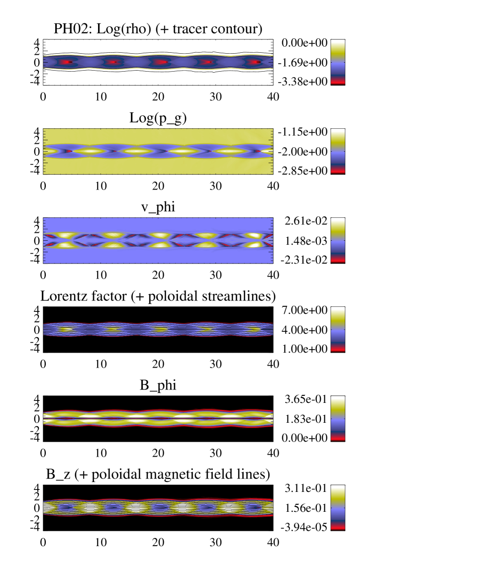
Figure 3.— Steady structure of the Poynting flux dominated, hot jet model PH02. From top to bottom, distributions of rest-mass density, gas pressure, toroidal flow velocity, flow Lorentz factor, and toroidal and axial magnetic field components once the steady state has been settled. Poloidal flow and magnetic field lines are overimposed onto the Lorentz factor and axial magnetic field panels, respectively. Two contour lines for jet mass fraction values 0.005 and 0.995 are overplotted on the density panel.

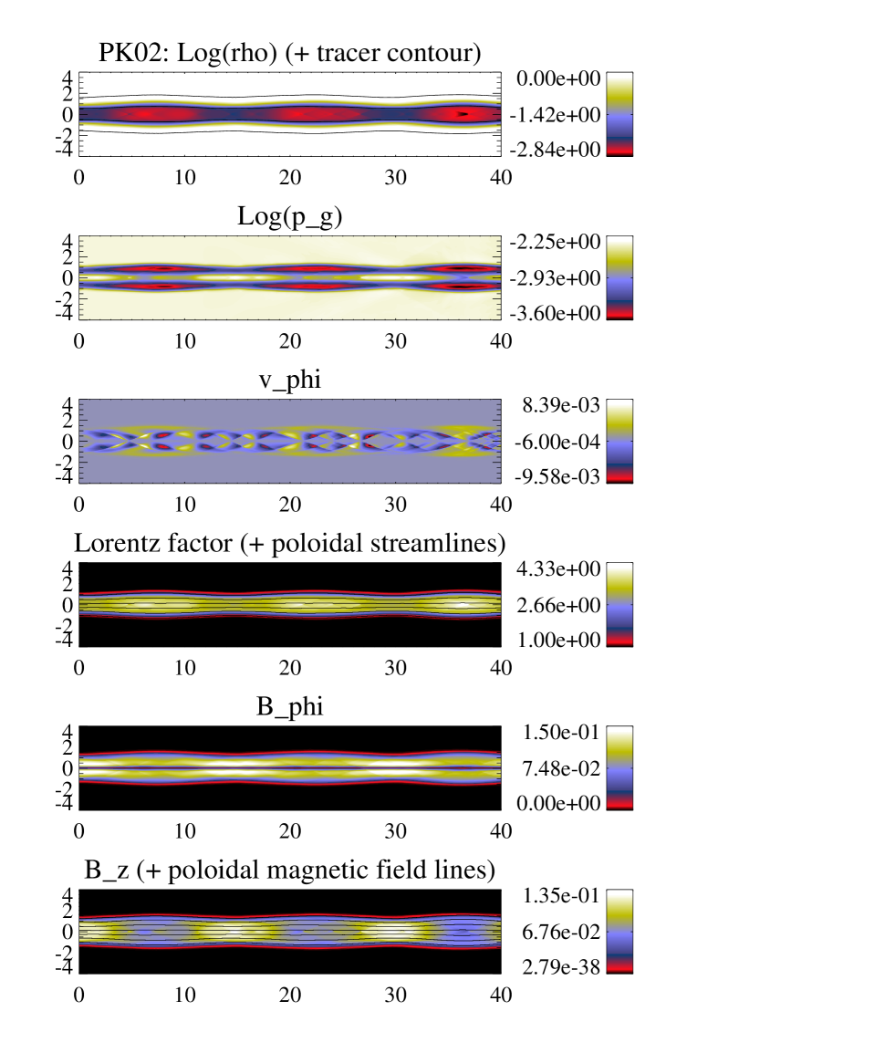
Figure 4.— Steady structure of the Poynting flux dominated jet model PK02. Panel distribution as in Fig. 3.

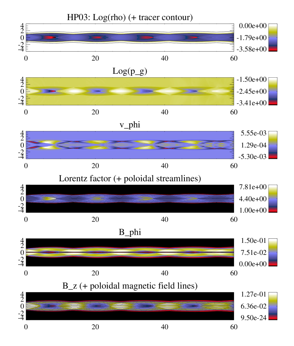
Figure 5.— Steady structure of the hot jet model HP03. Panel distribution as in Fig. 3.

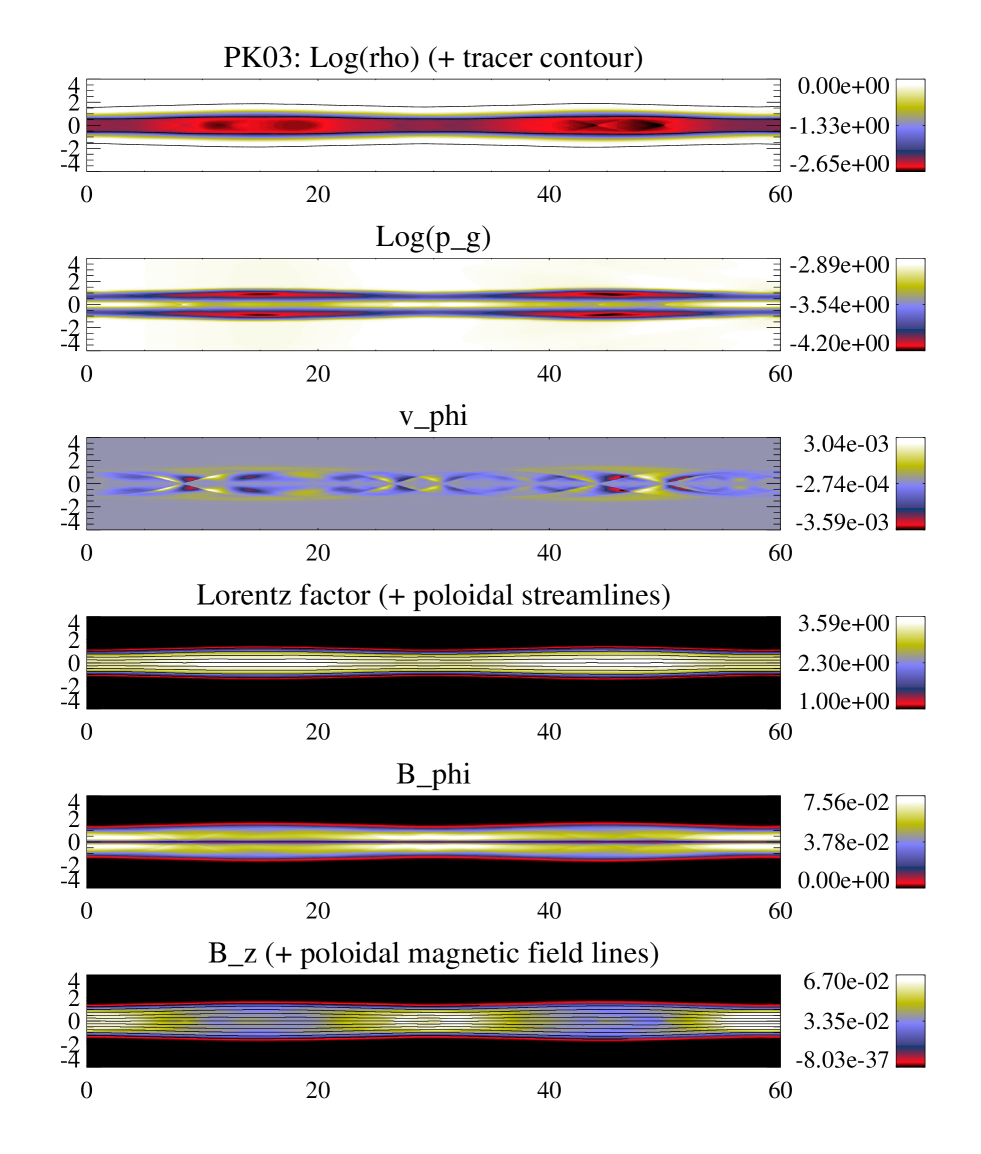
Figure 6.— Steady structure of the Poynting flux dominated jet model PK03. Panel distribution as in Fig. 3.

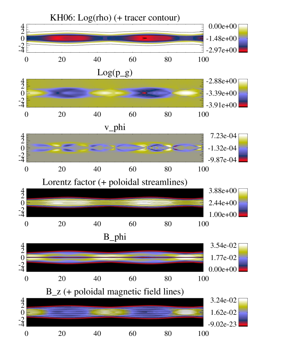
Figure 7.— Steady structure of the kinetically dominated jet model KH06. Panel distribution as in Fig. 3. Note that the axial scale has been compressed by a factor of 2 with respect to the radial one.

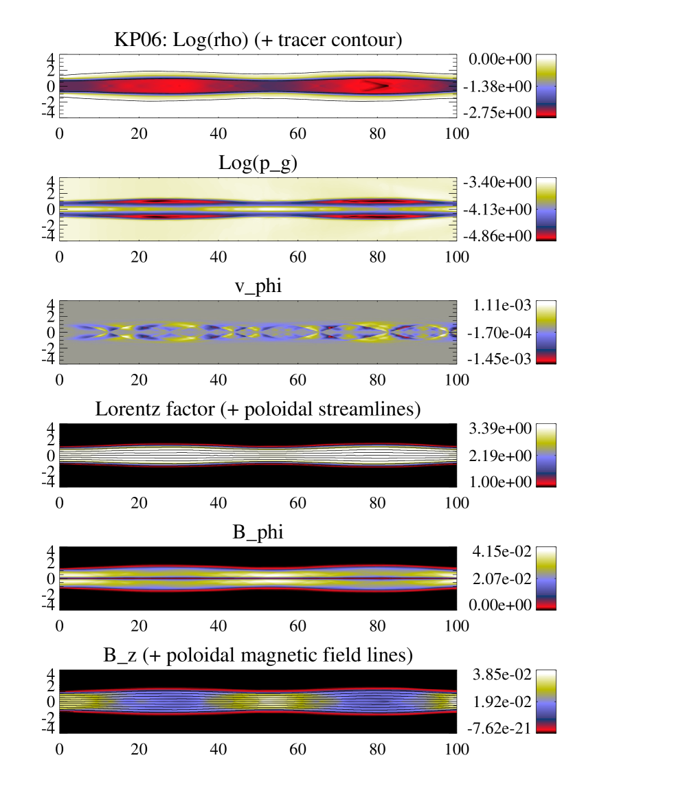
Figure 8.— Steady structure of the kinetically dominated, highly magnetized jet model KP06. Panel distribution as in Fig. 3. Note that the axial scale has been compressed by a factor of 2 with respect to the radial one.

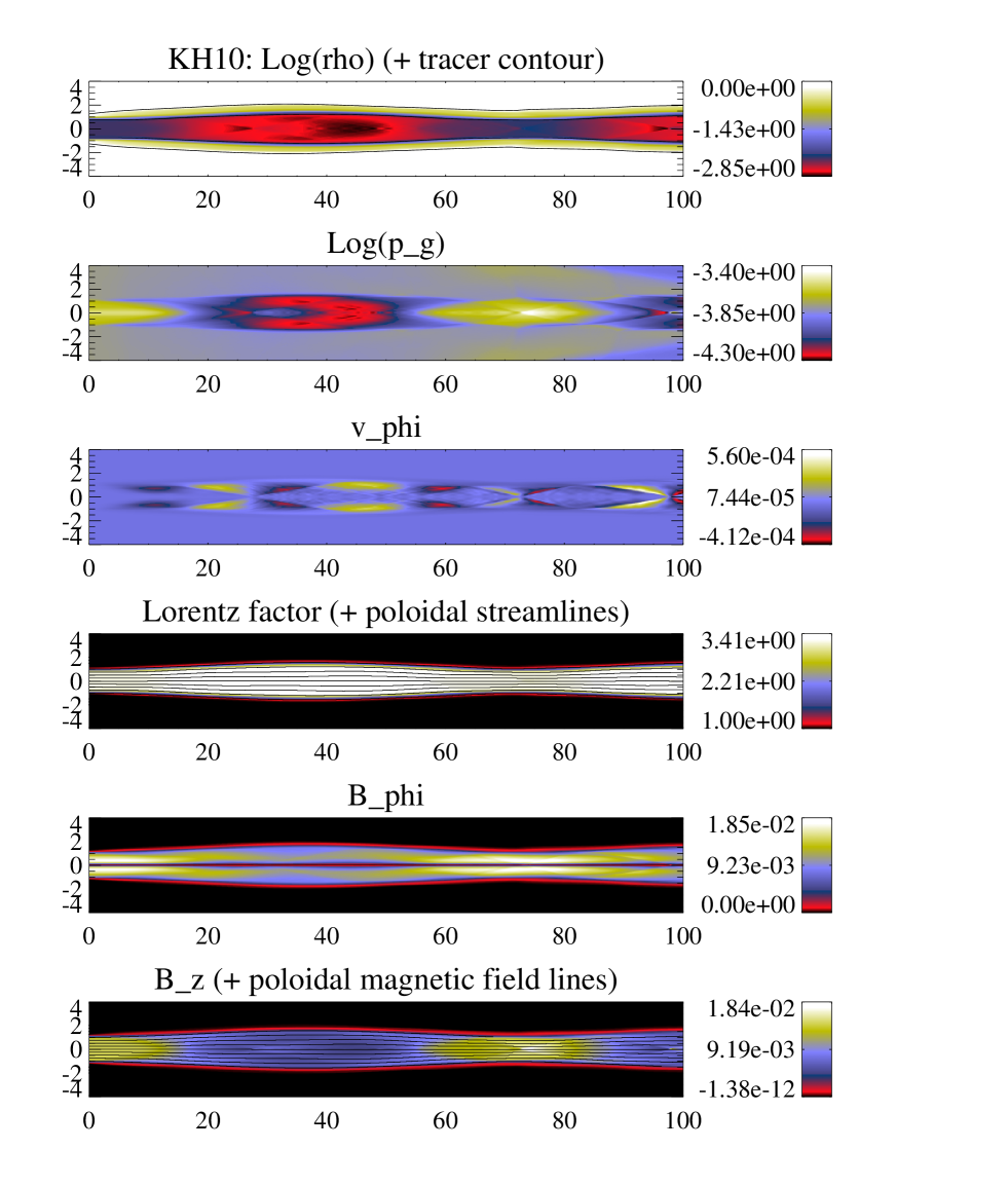
Figure 9.— Steady structure of the kinetically dominated jet model KH10. Panel distribution as in Fig. 3. Note that the axial scale has been compressed by a factor of 2 with respect to the radial one.

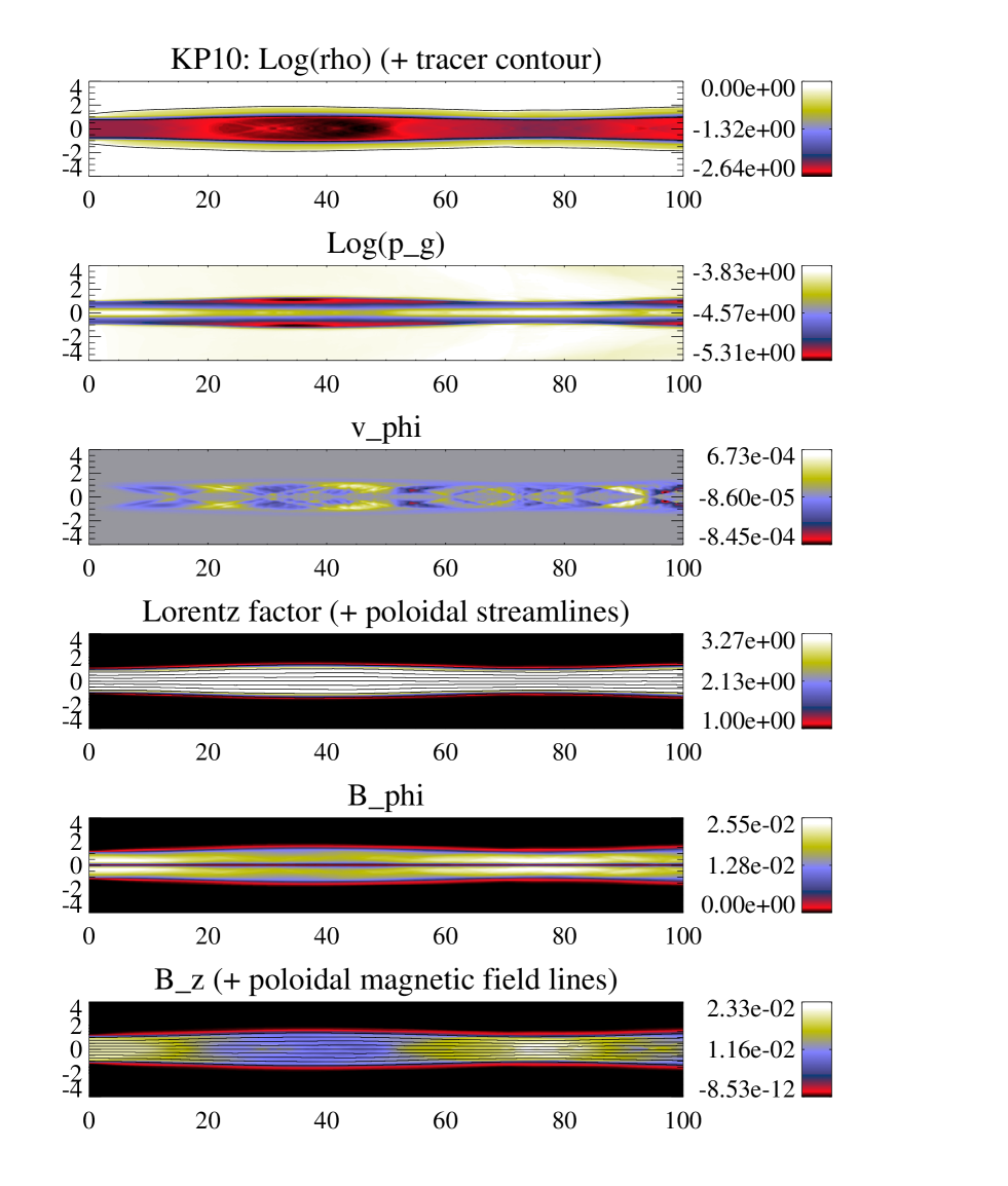
Figure 10.— Steady structure of the kinetically dominated, highly magnetized jet model KP10. Panel distribution as in Fig. 3. Note that the axial scale has been compressed by a factor of 2 with respect to the radial one.

Table 2Averaged values and relative variations along the jet of the quantities defining the steady models. $\Delta z$ stands for the wavelength associated to the jet oscillation along the axis. Remaining symbols, as defined in Sect. 2.

Modela	$\bar{R}\,[R_{j}]$	$\displaystyle{\frac{\Delta R}{\bar{R}}}$	$\bar{\rho}\,[\rho_{a}]$	$\displaystyle{\frac{\Delta\rho}{\bar{\rho}}}$	$\bar{\varepsilon}\,[c^{2}]$	$\displaystyle{\frac{\Delta\varepsilon}{\bar{\varepsilon}}}$	$\bar{\beta}$	$\displaystyle{\frac{\Delta\beta}{\bar{\beta}}}$	$\bar{\phi}\,[^{\circ}]$	$\displaystyle{\frac{\Delta\phi}{\bar{\phi}}}$	$\bar{W}$	$\displaystyle{\frac{\Delta W}{\bar{W}}}$	$\Delta z^{b}\,[R_{j}]$
PH02s	$1.00$	$0.26$	$0.0034$	$0.74$	$9.00\phantom{00}$	$0.24$	$2.67$	$0.02$	$51.71$	$0.19$	$3.69$	$0.22$	$\phantom{0}8.0$
PH02j	$1.20$	$0.25$	$0.060\phantom{0}$	$0.43$	$6.56\phantom{00}$	$0.14$	$2.25$	$0.06$	$51.19$	$0.18$	$3.18$	$0.24$	$\phantom{0}8.0$
PK02s	$0.64$	$0.23$	$0.0045$	$0.64$	$0.76\phantom{00}$	$0.24$	$6.19$	$0.21$	$52.05$	$0.15$	$3.34$	$0.09$	$14.5$
PK02j	$1.22$	$0.20$	$0.16\phantom{00}$	$0.40$	$0.23\phantom{00}$	$0.11$	$6.27$	$0.12$	$48.55$	$0.14$	$2.29$	$0.13$	$14.5$
HP03s	$1.03$	$0.29$	$0.0032$	$0.91$	$8.31\phantom{00}$	$0.28$	$0.44$	$0.02$	$52.25$	$0.21$	$3.77$	$0.27$	$13.8$
HP03j	$1.25$	$0.24$	$0.050\phantom{0}$	$0.52$	$5.93\phantom{00}$	$0.19$	$0.37$	$0.11$	$51.35$	$0.21$	$3.24$	$0.28$	$13.8$
PK03s	$0.65$	$0.23$	$0.0046$	$0.63$	$0.20\phantom{00}$	$0.25$	$6.08$	$0.25$	$52.05$	$0.13$	$3.24$	$0.03$	$30.0$
PK03j	$1.23$	$0.21$	$0.16\phantom{00}$	$0.44$	$0.060\phantom{0}$	$0.13$	$6.13$	$0.18$	$48.61$	$0.19$	$2.24$	$0.09$	$30.0$
KH06s	$1.09$	$0.46$	$0.0030$	$1.20$	$0.37\phantom{00}$	$0.43$	$0.40$	$0.45$	$55.43$	$0.31$	$3.45$	$0.17$	$38.0$
KH06j	$1.57$	$0.38$	$0.037\phantom{0}$	$0.84$	$0.201\phantom{0}$	$0.25$	$0.25$	$0.28$	$54.22$	$0.28$	$2.60$	$0.23$	$38.0$
KP06s	$0.82$	$0.24$	$0.0041$	$0.76$	$0.042\phantom{0}$	$0.24$	$7.69$	$0.39$	$52.82$	$0.20$	$3.20$	$0.02$	$53.0$
KP06j	$1.27$	$0.30$	$0.097\phantom{0}$	$0.41$	$0.019\phantom{0}$	$0.13$	$6.73$	$0.22$	$50.00$	$0.20$	$2.42$	$0.08$	$53.0$
KH10s	$0.96$	$0.47$	$0.0036$	$0.97$	$0.11\phantom{00}$	$0.33$	$0.41$	$0.44$	$53.90$	$0.26$	$3.25$	$0.05$	$74.0$
KH10j	$1.37$	$0.40$	$0.065\phantom{0}$	$0.78$	$0.058\phantom{0}$	$0.17$	$0.32$	$0.31$	$51.67$	$0.25$	$2.54$	$0.14$	$70.0$
KP10s	$0.88$	$0.32$	$0.0042$	$0.62$	$0.016\phantom{0}$	$0.25$	$8.96$	$0.38$	$51.74$	$0.19$	$3.19$	$0.00$	$76.0$
KP10j	$1.28$	$0.27$	$0.071\phantom{0}$	$0.51$	$0.0084$	$0.14$	$6.83$	$0.20$	$49.49$	$0.20$	$2.48$	$0.08$	$72.0$

^a Two rows per model are displayed. The first row (label s) shows values in the jet spine, defined as the region of the jet around the axis with jet mass fraction $f\geq 0.995$. The second row (label j) shows averages for the whole jet ($f>0$).
^b $\Delta z$ stands for the wavelength of the jet oscillation along the jet axis.

The internal structure of the jets will be now analyzed and compared with the help of Figs. 3 to 10 and the results given in Table 2.

1. The models with a richer internal structure are those dominated by the internal energy, i.e., those in the hot models region or its neighbourhood (i.e., Poynting-flux dominated jets with relatively small magnetization), PH02 and HP03. In these cases, the models have a substantial amount of internal energy which is efficiently converted into kinetic energy at jet expansions and back to internal energy at recollimation shocks. These models present the largest variations in flow Lorentz factor. The maximum Lorentz factor in model PH02 is 7.0 (2.19 times its initial value; see Fig. 3) and the change in the average values is of 22-24% (see Table 2). In the case of model HP03, the maximum Lorentz factor is 7.81 (2.44 times its initial value) and the change in the average values is of 27-28%. Associated to these variations in the flow Lorentz factor is the variation of the internal energy density along the axis. In the case of model PH02, this variation is a factor of $\approx 50$. For model HP03, it is a factor of $\approx 80$.

2. Kinetically dominated jets (KH06 to KP10) are dominated by the rest-mass energy density and the inertia of the flow in these models is very large. In these models, specially in the colder ones (KH10, KP10), there is not much internal nor magnetic energy to be converted into kinetic one and the jets have no internal structure. In models KH10 and KP10 the maximum Lorentz factor is only 1.02-1.06 times the initial value (see Figs. 8 and 10) and the change in the average values on the spine of the jets is smaller than 2% (8% including the shear layer; see Table 2).

3. Models PK02, PK03 are Poynting-flux dominated models with high magnetization ($\beta_{j}=10$) and large magnetic pitch angles ($\phi_{j}=45^{\circ}$). In these cases, the width of the shear layer required to reduce the growth rate of the magnetic pinch modes could affect the internal structure of the models (see the discussion at the beginning of this section).

4. The wavelength of the jet oscillation, $\Delta z$ (see Table 2), increases with increasing magnetosonic Mach number, as expected from the decrease of the Mach angle. This happens both for constant specific internal energy (and decreasing magnetization), and constant magnetization (and decreasing specific internal energy). Finally, for constant magnetosonic Mach number, this wavelength increases for decreasing specific internal energy (or increasing magnetization). Kinetically dominated jets tend to have the longest wavelengths. In the models with the highest specific internal energies the oscillation of the jet leads to a series of recollimation shocks of the same periodicity. The angle formed by these conical shocks with the jet axis is of $\approx 18^{\circ}$ for model PH02 and $\approx 12^{\circ}$ for model HP03 (see below).

5. Finally, the change in magnetic pitch angle for all models is limited to a mere 25-26% corresponding to a variation of $\pm 6^{\circ}$ around the average value.

5.3. Standing shocks

Standing oblique discontinuities (recollimation shocks) can be distinguished in some of the jets, specially in hot models (PH02, HP03) and, to a lesser extent, in colder, low magnetization models (KH06, KH10).

The characterization of discontinuities in a magnetized fluid can be done through the jumps of the different variables across them (see the books by Lichnerowicz, 1967; Anile, 1989, for a complete discussion). Taking into account that across a shock the specific entropy increases, $s_{b}>s_{a}$ (where subscripts $a$ and $b$ refer to the state ahead and behind the shock, respectively), the compressibility assumptions $\partial(h/\rho)/\partial p|_{s}<0$, $\partial(h/\rho)/\partial s|_{p}>0$, $\partial^{2}(h/\rho)/\partial p^{2}|_{s}>0$, verified by the ideal gas describing the jet fluid, lead to $p_{b}>p_{a}$, $\rho_{b}>\rho_{a}$, $h_{b}>h_{a}$ ($(h/\rho)_{b}<(h/\rho)_{a}$). Additionally, the magnetic pressure increases across a fast magnetosonic shock, $p_{m,b}>p_{m,a}$, and decreases across a slow magnetosonic shock, $p_{m,b}<p_{m,a}$. Finally, the increase in density across a shock, coincides with a decrease in the flow speed (or in the spatial component of the four-velocity) in the shock rest-frame.

In a unsteady flow, identifying the states ahead and behind a shock can be a difficult task. However in our steady jet models, fluid particles enter the hypothetical discontinuities from the left (smaller axial coordinate $z$) and leave them from the right (larger $z$). With all this in mind we have built a detector of superfast magnetosonic shocks based on the gradients of the thermal and magnetic pressures and the divergence of velocity. The results are shown in Figs. 11-14. These figures show the map of $d=|\Delta v_{-}|\Delta p_{+}\Delta p_{m,+}$, where $\Delta v_{-}$ is defined as the divergence of the three-velocity if it is negative, and zero otherwise, and $\Delta p_{+}$ and $\Delta p_{m,+}$, as the corresponding gradients of the thermal, $p$, and magnetic, $p_{m}$, pressure if the $z$ components of the gradient are positive (and zero otherwise). According to our analysis, the internal structures seen in the color panels of the different models (Figs. 3-10) are identified as fast magnetosonic shocks in Figs. 11-14.

Some conclusions can be drawn from these figures. Models PH02 and HP03 (corresponding to the hottest jets studied and with the thinnest shear layer) and to a lesser extent models KH06 and KH10 (kinetically dominated jet models) display a series of periodic recollimation shocks associated with the jet sideways oscillations. In the remaining models (Poynting-flux dominated models with the widest shear layer), the primary shocks associated with the oscillations of the jet are weaker and dilute in a more complex structure of shocks (and compression waves). All the standing shocks in a jet form the same angle with respect to the jet axis and there is a clean correlation between the shock angle (the angle formed by the conical shock and the jet axis) and the magnetosonic Mach number (see Table 3).

Finally, let us note that none of our models display Mach disks. This kind of structures replace conical shocks when the shocks are strong enough. Since in our simulations the strength of the standing shocks depends on the jet overpressure factor, we would expect to find Mach disks for larger overpressure factors.

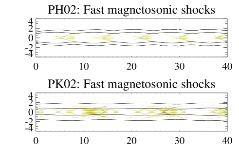
Figure 11.— Fast magnetosonic shocks in models PH02 and PK02 (${\cal M}_{ms,j}=2.0$).

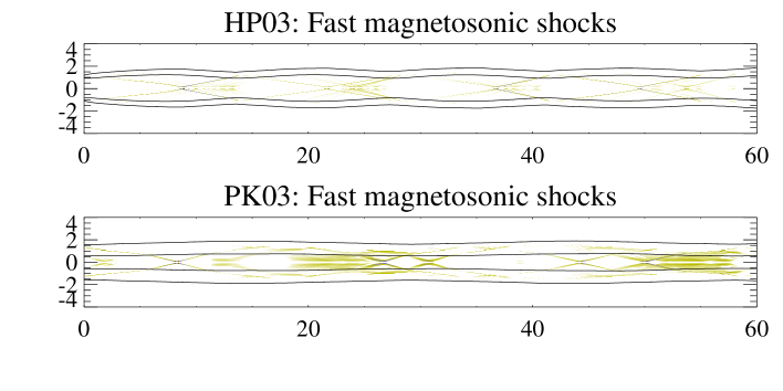
Figure 12.— Fast magnetosonic shocks in models HP03 and PK03 (${\cal M}_{ms,j}=3.5$).

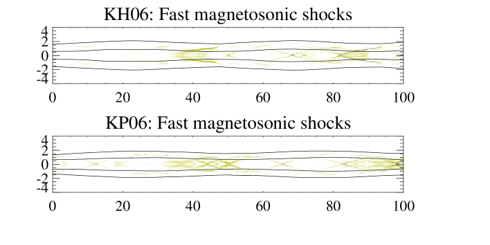
Figure 13.— Fast magnetosonic shocks in models KH06 and KP06 (${\cal M}_{ms,j}=6.0$). Note that the axial scale has been compressed by a factor of 2 with respect to the radial one.

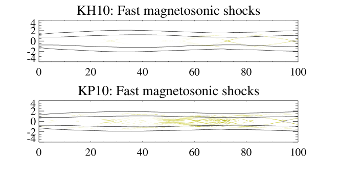
Figure 14.— Fast magnetosonic shocks in models KH10 and KP10 (${\cal M}_{ms,j}=10.0$). Note that the axial scale has been compressed by a factor of 2 with respect to the radial one.

Table 3Shock angle, $\phi_{s}$, as a function of the magnetosonic Mach number, ${\cal M}_{ms}$. The Mach angle, $\phi_{M}=\arctan(1/{\cal M}_{ms})$ is also shown for comparison.

${\cal M}_{ms}$	$\phi_{M}$ [∘]	$\phi_{s}$ [∘]
2.0	26.6	18 $\pm$ 1
3.5	15.9	13 $\pm$ 1
6.0	9.5	8 $\pm$ 1
10.0	5.7	6 $\pm$ 1

5.4. Astrophysical applications

The correlation found in our simulations between the Mach angles, the angles of the recollimation shocks and the separation between them (in models with internal structure) allows us to estimate the Mach numbers of parsec-scale jets with stationary components.

Based on multifrequency VLBI observations in the period May 2005-April 2007, Fromm et al. (2013a) report on the properties of three quasi-stationary components (B1, B2 and B3) located between 4 and 7 mas from the core of CTA 102. Taking these components as standing shocks, the shock angle can be estimated as the angle subtended by the jet diameter at a distance equal to the shock separation. Our study is based on the 15GHz observations made on 8th of June 2006 (see Tables A.3 and A.6, and Figs. A.7 and A.8 in Fromm et al., 2013a, for the component analysis at 15 GHz). Assuming the mean of the size of a pair of consecutive components (estimated as the FWHM of the corresponding fitting Gaussians) as a lower bound of the jet diameter between these components, and the corresponding shock separation (correcting projection effects for a viewing angle of 2.6^∘, Jorstad et al., 2005), we find an upper bound for the Mach number of 31.8 for the flow between B3 and B2 components, and correspondingly of 34.2 for the flow between B2 and B1. For an estimated flow Lorentz factor of 10 (from the apparent speeds estimated in the neighbour regions A and D; see Table 3 and Fig. 13 of Fromm et al., 2013a), the values obtained for the Mach number upper bounds would fall into the kinetically dominated jet region of the corresponding magnetosonic Mach number-specific internal energy plot, indicating that the jet can be kinetically dominated at distances $\approx 720-1260$ pc ($0.1$ mas in projection $\approx$ $18$ pc deprojected) from the central source (see below).

We can apply the same analysis to the quasi-steady components inside the innermost jet regions in BL Lacertae, recently reported by Gómez et al. (2016). From the component separation and component sizes (estimated again as the FWHM of the corresponding Gaussian fits) at 43 GHz for the core and components Q1 and Q2 (see Table 2 and Fig. 3 of Gómez et al., 2016), and a viewing angle of 8^∘ (Jorstad et al., 2005), we can derive upper bounds for the Mach numbers of the flow between the core and component Q1, 17.5, and between components Q1 and Q2, 19.4. For an estimated flow Lorentz factor of 7 (Jorstad et al., 2005), the Mach numbers bounds lie again in the kinetically dominated region but closer to the hot/Poynting flux dominated region boundary, at $\approx 2.4$ pc ($0.1$ mas in projection $\approx$ $0.97$ pc deprojected) from the central source. The parameters used in Gómez et al. (2016) to simulate the jet in BL Lac corresponding to a hot, low-magnetization jet, are consistent with our estimations.

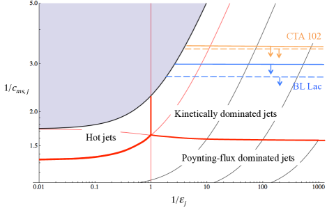
Figure 15.— Classical magnetosonic Mach number estimates for the jets of CTA 102 and BL Lacertae on the $1/c_{ms,j}-1/\varepsilon_{j}$ plane and distribution of jet models according to the dominant energy type. The black and red lines appearing in this diagram have the same meaning as the corresponding ones in Fig. 1. The yellow (blue) solid and dashed lines give maximum values for the two estimates of the Mach number in the jet of CTA 102 (BL Lac), as discussed in the text.

The Mach number estimates for CTA 102 and BL Lacertae are shown in Fig. 15, equivalent to the top panel in Fig. 1, but replacing the relativistic magnetosonic Mach number in the ordinate axis by the inverse of the magnetosonic speed ($c_{ms}$; see Appendix A), a very good approximation of the classical counterpart of the magnetosonic Mach number for high Lorentz factor flows. It is interesting to note that our estimates of the dominant type of energy for the jets of BL Lacertae and CTA 102 fits well within the current paradigm of jet acceleration, in which jets would form at some point in the hot/Poynting-flux dominated region and would evolve towards the region of kinematically dominated models. This trend would have to be confirmed with a larger sample of sources with stationary components and estimates of the bulk flow Lorentz factor and jet viewing angle. However we should note that the present approach for the estimation of the dominant type of energy in the jet is applicable only to jets displaying stationary components.

6. Summary and conclusions

The internal structure of eight superfast magnetosonic, overpressured jet models has been analyzed. The injection parameters of these models have been chosen to cover a wide region in the magnetosonic Mach number - specific internal energy plane. The merit of this plane is that models dominated by different kind of energies (internal energy: hot jets; rest-mass energy: kinetically dominated jets; magnetic energy: Poynting-flux dominated jets) occupy well separated regions. The analyzed models also cover a wide range of magnetizations. The rest of injection parameters (the rest-mass density, the jet overpressure factor, the flow Lorentz factor, and the flow azimuthal velocity -equal to zero-) are kept constant.

Jets are injected in internal transversal equilibrium to minimize the sideways perturbations once immersed in the ambient medium and to obtain an internal structure as clean as possible. The transition between the jet and the ambient medium is smoothed by means of a shear layer of different widths to stabilize the models against the growth of magnetic pinch instabilities. The conclusions of our analysis are listed below.

1. The models with a richer internal structure are those dominated by the internal energy, i.e., those in the hot jets region or its neighbourhood (i.e., Poynting-flux dominated jets with magnetizations larger than but close to 1). In these cases, the models have a substantial amount of internal energy which is efficiently converted into kinetic energy at jet expansions and back to internal energy at recollimation shocks. These models present the largest variations in flow Lorentz factor and internal energy density along the axis.

2. Conversely, in the kinetically dominated jet models there is not much internal nor magnetic energy to be converted into kinetic one, the jets have no internal structure and the flow Lorentz factor is constant. Despite the large difference in magnetization, kinetically dominated models with the same magnetosonic Mach number have very similar overall structure (jet oscillation, amplitude of variations, local jet opening angles,…).

3. As a consequence of the magnetic pinch exerted by the toroidal magnetic field, models with large magnetizations concentrate most of their internal energy in a thin hot spine around the axis. The width of this spine is related with the location of the maximum toroidal field across the jet.

4. Poynting-flux dominated models with high magnetization are prone to be unstable against magnetic pinch modes.

5. All the models present a jet oscillation with a characteristic wavelength that follows definite trends with specific internal energy, magnetosonic Mach number and magnetization.

6. The change in (average) magnetic pitch angle is limited to few degrees around the average value. However, large local radial variations in the pitch angle can be expected from almost $0^{\circ}$ close to the axis to values larger than the average at some intermediate radius.

7. Despite the fact that the studied models are injected with pure axial flow velocities, all develop small azimuthal velocities (of the order of 2% of the speed of light or smaller) as a result of the Lorentz force in axisymmetric converging/diverging flows. These speeds tend to be larger in those models where the jet oscillation has a larger amplitude.

Despite its limitations, the present study is the first attempt to identify the structural ingredients (including the properties of recollimation shocks) that characterize hot, Poynting-flux dominated and kinetically dominated, relativistic jets. Our study is of special relevance in the interpretation of parsec-scale AGN jets. On one hand, our simulations confirm the correlation between the Mach angles, the angles of the conical shocks and the separation between them (in models with internal structure) and allow us to estimate the magnetosonic Mach numbers of parsec-scale jets with stationary components. It should be noted, however, that our simulations are two-dimensional and that imperfect azimuthal symmetry of the ambient medium would disrupt the coherence of the standing shock pattern after few jet oscillations. On the other hand, our study reveals that the presence of a significant toroidal component of the magnetic field in these objects produces a complex transversal structure with a central spine (extending up to the radius of the maximum of the toroidal field) where the thermal pressure (and hence the plasma internal energy) is close to its maximum. A layer with milder (magnetic, thermal) pressure profiles that extends up to the outer jet/ambient-medium transition layer wraps the central spine. This complex profile in the thermal energy distribution and the magnetic pitch angle must leave their imprints in the total and polarized emission, which will be the subject of a forthcoming paper. In that work we shall analyze in detail the emission properties of these models, paying special attention to the relative intensity of the components associated to the shocks as a function of the viewing angle, to the tranversal structure of the jet and, in general, to the signatures of the magnetic field structure in the polarized emission.

Our results prove the stabilization effect of shear layers for the CDI in Poynting-flux dominated jets. More interestingly, the stability of Poynting flux dominated jets against pinch oscillations (and, in particular, the role of the shear layer in the stabilization of these flows) merits further exploration as a way to constrain the magnetization parameter and/or the magnetic field configuration in parsec-scale AGN jets.

Additional parameters should be explored, specially the overpressure factor (related with the formation of Mach disks) and the magnetic field pitch angle, as well as new strategies to generate the steady models. In a recent paper, Komissarov, Porth & Lyutikov (2015) describe a simple numerical approach to study the structure of steady axisymmetric superfast-magnetosonic jets by means of one-dimensional time dependent simulations by using $z$ (the axial cylindrical coordinate) as the time coordinate. Although subject to a number of approximations, the approach works well and could be used to generate approximate steady solutions in a wider space of parameters.

Appendix A Appendix A. Characteristic wavespeed diagrams for the RMHD

The characteristic wave speed diagrams (Antón et al., 2010), or phase polar diagrams (Cohen et al., 2015), show the normal speed of planar wave fronts propagating in different directions, the speed given by the distance between the origin and the normal speed surface along the corresponding direction. These speeds correspond to the phase speeds of linear perturbations studied by Keppens & Meliani (2008). The two panels of Fig. 16 display the characteristic wavespeed surfaces of fast magnetosonic waves ($\lambda_{F}$, in blue), Alfvén waves ($\lambda_{A}$, in yellow), slow magnetosonic waves ($\lambda_{S}$, in red) and entropy waves (the point at the origin) for the homogeneous states of a magnetized ideal gas in the fluid rest frame corresponding to models PH02 and KH10. The jet axis is along the $x$ axis, whereas the oblique discontinuous straight line is along the average helical magnetic field (in the fluid rest frame).

Distinctly to sound waves, magnetosonic waves are anisotropic, with the propagation speeds $\lambda_{S}$, $\lambda_{F}$ and $\lambda_{A}$ depending on the angle, $\chi$, of the propagation direction and the magnetic field

$$\lambda_{A}(\chi)=c_{A}\cos\chi$$ (A1)

$$\lambda_{F,S}(\chi)=\pm\sqrt{\frac{1}{2}\left[d(\chi)^{2}\pm(d(\chi)^{4}-4c_{s}^{2}c_{A}^{2}\cos^{2}\chi)^{1/2}\right]}$$ (A2)

In these expressions, $d(\chi)^{2}=c_{s}^{2}+c_{A}^{2}-c_{s}^{2}c_{A}^{2}\sin^{2}\chi$, where $c_{s}$ ($=\sqrt{\gamma p/\rho h}$, for an ideal gas with adiabatic index $\gamma$) is the sound speed, and $c_{A}$ the Alfvén speed

$$c_{A}=\sqrt{\frac{b^{2}}{\rho h+b^{2}}}.$$ (A3)

An homogeneous flow is said to be super-fast magnetosonic if the flow velocity, $v$, is $v>\lambda_{F}(\chi)$, where $\chi$ is the angle between the flow propagation direction and the magnetic field in the fluid rest frame. For practical purposes, we shall define our superfast-magnetosonic jets as those for which $v_{j}>c_{ms,\,j}$, with $c_{ms}$, the magnetosonic speed (discontinuous blue line in Fig. 16), being

$$c_{ms}=\sqrt{c_{A}^{2}+c_{s}^{2}(1-c_{A}^{2})}.$$ (A4)

It can be seen that $c_{ms}\geq\lambda_{F}(\chi)$, $\forall\chi$. In low magnetization jets, $\displaystyle{\beta=\frac{b^{2}}{2p}}$ is very small, which means that $c_{A}\ll c_{s}$ (see Eq. A3) and $c_{ms}\approx c_{s}$ (see Eq. A4).

Associated with the the superfast-magnetosonic flow is the magnetosonic Mach number (see Cohen et al. 2015)

$${\cal M}_{ms}=\frac{W}{W_{ms}}\frac{v}{c_{ms}},$$ (A5)

where $W$ is the flow Lorentz factor and $W_{ms}$ is the flow Lorentz factor associated to the magnetosonic speed. In low magnetization jets, the magnetosonic Mach number coincides with the common (sound) Mach number.

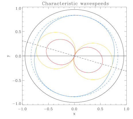
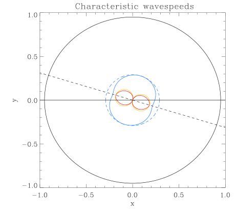
Figure 16.— Left panel: Characteristic wavespeed surfaces of fast magnetosonic waves (in blue), Alfvén waves (in yellow), slow magnetosonic waves (in red) and entropy waves (the point at the origin) for the homogeneous state of a magnetized ideal gas in the fluid rest frame corresponding to models PH02. The jet axis is along the $x$ axis, whereas the oblique discontinuous straight line is along the average helical magnetic field (in the fluid rest frame). The black circumference represents the flow propagation velocity. Right panel: The same as the left panel but for the homogeneous state corresponding to KH10.

References

- Anile (1989) Anile, A.M., Relativistic fluids and magneto-fluids, Cambridge: Cambridge University Press, 1989
- Antón et al. (2010) Antón, L., Miralles, J.A., Martí, J.M., Ibáñez, J.M., Aloy, M.A., & Mimica, P. 2010, ApJS, 188, 1
- Appl, Lery & Baty (2000) Appl, S., Lery, T., & Baty, H. 2000, Astron. Astrophys., 355, 818
- Blandford & Königl (1979) Blandford, R. D., & Königl, A. 1979, ApJ, 232, 34
- Blandford & Payne (1982) Blandford, R. D., & Payne, D. G. 1982, MNRAS, 199, 883
- Blandford & Znajek (1977) Blandford, R. D., & Znajek, R. L. 1977, MNRAS, 179, 433
- Casadio et al. (2015a) Casadio, C., Gómez, J. L., Jorstad, S. G., et al. 2015a, ApJ, 813, 51
- Casadio et al. (2015b) Casadio, C., Gómez, J. L., Grandi, P., et al. 2015b, ApJ, 808, 162
- Cohen et al. (2014) Cohen, M. H., Meier, D. L., Arshakian, T. G., et al. 2014, ApJ, 787, 151
- Cohen et al. (2015) Cohen, M.H., Meier, D. L., Arshakian, T. G., et al. 2015, ApJ, 803, 3
- Daly & Marscher (1988) Daly, R. A. & Marscher, A. P. 1988, ApJ, 334, 539
- Dubal & Pantano (1993) Dubal, M. R., & Pantano, O. 1993, MNRAS, 261, 203
- Fromm et al. (2011) Fromm, C. M., Perucho, M., Ros, E., et al. 2011, Astron. Astrophys., 531, A95
- Fromm et al. (2013a) Fromm, C.M., Ros, E., Perucho, M., et al. 2013, Astron. Astrophys., 551, A32
- Fromm et al. (2013b) Fromm, C.M., Ros, E., Perucho, M., et al. 2013, Astron. Astrophys., 557, A105
- Fromm et al. (2016) Fromm, C.M., Perucho, M., Mimica, P., & Ros, E. 2016, Astron. Astrophys., 588, A101
- Gómez et al. (2016) Gómez, J.L., Lobanov, A. P., Bruni, G., et al. 2016, ApJ, 817, 96
- Gómez et al. (1997) Gómez, J. L., Martí, J. M., Marscher, A. P., Ibáñez, J. M., & Alberdi, A. 1997, ApJ, 482, L33
- Gómez et al. (1995) Gómez, J. L., Martí, J. M., Marscher, A. P., Ibáñez, J. M., & Marcaide, J. M. 1995, ApJ, 449, L19
- Hardee (2011) Hardee, P. E. 2011, The stability of astrophysical jets, in Jets at all scales, Proc. of the 275 IAU Symposium, eds. G. E. Romero, R. A. Sunyaev, T. Belloni, Cambridge: Cambridge University Press, p. 41.
- Hardee & Rosen (2002) Hardee, P. E. & Rosen, A. 2002, ApJ, 576, 204
- Ibáñez et al. (2013) Ibáñez, J.M., Cordero-Carrión, I., Martí, & J.M. Miralles, J.A. 2013, Class. Quantum Grav., 30, 057002
- Jorstad et al. (2005) Jorstad, S.G. et al. 2005, AJ, 130, 1418
- Keppens & Meliani (2008) Keppens, R., & Meliani, Z. 2008, Physics of Plasmas, 15, 102103
- Kim et al. (2015) Kim, J., Balsara, D.S., Lyutikov, M., et al. 2015, MNRAS, 450, 982
- Kim et al. (2016) Kim, J., Balsara, D.S., Lyutikov, M., et al. 2016, MNRAS, in press, arXiv:1603.00341 [astro-ph.HE]
- Komissarov (1999) Komissarov, S.S. 1999, MNRAS, 303, 343
- Komissarov et al. (2007) Komissarov, S. S., Barkov, M. V., Vlahakis, N., & Königl, A. 2007, MNRAS, 380, 51
- Komissarov & Falle (1997) Komissarov, S. S., & Falle, S. A. E. G. 1997, MNRAS, 288, 833
- Komissarov, Porth & Lyutikov (2015) Komissarov, S.S., Porth, O., & Lyutikov, M. 2015, Comput. Astrophys. Cosmology, 2, 9
- Leismann et al. (2005) Leismann, T. et al. 2005, Astron. Astrophys., 436, 503
- Lichnerowicz (1967) Lichnerowicz, A., Relativistic hydodynamics and magnetohydrodynamics, New York: Benjamin, 1967
- Lind et al. (1989) Lind, K.R., Payne, D.G., Meier, D.L., & Blandford, R.D. 1989, ApJ, 344, 89
- Marscher et al. (2008) Marscher, A. P., Jorstad, S. G., D’Arcangelo, F. D., et al. 2008, Nature, 452, 966
- Marscher et al. (2010) Marscher, A. P., Jorstad, S. G., Larionov, V. M., et al. 2010, ApJ, 710, L126
- Martí (2015) Martí, J.M. 2015, MNRAS, 452, 3106
- Martí et al. (1997) Martí, J.M., Müller, E., Font, J.A., Ibáñez, J.M., & Marquina, A. 1997, ApJ, 479, 151
- Matsumoto, Masada & Shibata (2012) Matsumoto, J., Masada, Y., & Shibata, K. 2012, ApJ, 751, 140
- McKinney & Blandford (2009) McKinney, J. C., & Blandford, R. D. 2009, MNRAS, 394, L126
- Mimica et al. (2009) Mimica, P., Aloy, M. A., Agudo, I., et al. 2009, ApJ, 696, 1142
- Mizuno et al. (2015) Mizuno, Y. et al. 2015, ApJ, 809, 38
- Mizuno, Hardee & Nishikawa (2007) Mizuno, Y., Hardee, P. E., & Nishikawa, K.-I. 2007, ApJ, 662, 835
- Nakamura & Asada (2013) Nakamura, M., & Asada, K. 2013, ApJ, 775, 118
- Norman et al. (1982) Norman, M.L., Winkler, K.-H.A., Smarr, L., & Smidth, M.D. 1982, Astron. Astrophys., 113, 285
- Payne & Cohn (1985) Payne, D.G. & Cohn, D.G. 1985, ApJ, 291, 655
- Perucho et al. (2004) Perucho, M., Hanasz, M., Martí, J.M., & Sol, H. 2004, Astron. Astrophys., 427, 415
- Perucho et al. (2005) Perucho, M., Martí, J.M., & Hanasz, M. 2005, Astron. Astrophys., 443, 863
- Porth & Komissarov (2015) Porth, O., & Komissarov, S. S. 2015, MNRAS, 452, 1089
- Roca-Sogorb et al. (2010) Roca-Sogorb, M., Gómez, J. L., Agudo, I., Marscher, A. P., & Jorstad, S. G. 2010, ApJ, 712, L160
- Roca-Sogorb et al. (2008) Roca-Sogorb, M., Perucho, M., Gómez, J. L., Martí, J. M. Antón, L., Aloy, M. A., & Agudo, I. 2008, in Rector, T. A., De Young, D. S., eds, Extragalactic Jets: Theory and Observation from Radio to Gamma Ray ASP Conference Series, Vol. 386, p.488
- Roca-Sogorb et al. (2009) Roca-Sogorb, M., Perucho, M., Gómez, J. L., Martí, J. M. Antón, L., Aloy, M. A., & Agudo, I. 2009, in Hagiwara, Y., Fomalont, E., Tsuboi, M., Murata, Y., eds, Approaching Micro-Arcsecond Resolution with VSOP-2: Astrophysics and Technologies ASP Conference Series, Vol. 402, p.353
- Tchekhovskoy, Narayan & McKinney (2011) Tchekhovskoy, A., Narayan, R., & McKinney, J. 2011, MNRAS, 418, L79
- Wilson (1987) Wilson, M. J. 1987, MNRAS, 226, 447
- Zamaninasab et al. (2014) Zamaninasab, M., Clausen-Brown, E., Savolainen, T., & Tchekhovskoy, A. 2014, Nature, 510, 126