A comprehensive photometric study of dynamically evolved small van den Bergh-Hagen open clusters

Abstract

We present results from Johnson $UBV$, Kron-Cousins $RI$ and Washington $CT_{1}T_{2}$ photometries for seven van den Bergh-Hagen (vdBH) open clusters, namely, vdBH 1, 10, 31, 72, 87, 92, and 118. The high-quality, multi-band photometric data sets were used to trace the cluster stellar density radial profiles and to build colour-magnitude diagrams (CMDs) and colour-colour (CC) diagrams from which we estimated their structural parameters and fundamental astrophysical properties. The clusters in our sample cover a wide age range, from $\sim$ 60 Myr up to 2.8 Gyr, are of relatively small size ($\sim$ 1 $-$ 6 pc) and are placed at distances from the Sun which vary between 1.8 and 6.3 kpc, respectively. We also estimated lower limits for the cluster present-day masses as well as half-mass relaxation times ($t_{r}$). The resulting values in combination with the structural parameter values suggest that the studied clusters are in advanced stages of their internal dynamical evolution (age/$t_{r}$ $\sim$ 20 $-$ 320), possibly in the typical phase of those tidally filled with mass segregation in their core regions. Compared to open clusters in the solar neighbourhood, the seven vdBH clusters are within more massive ($\sim$ 80 $-$ 380M_⊙), with higher concentration parameter values ($c$ $\sim$ 0.75$-$1.15) and dynamically evolved ones.

1 Introduction

van den Bergh & Hagen (1975) performed a uniform survey over a $\sim$ 12$\degr$ strip of the southern Milky Way extending from l $\approx$ 250$\degr$ and l $\approx$ 360$\degr$. They employed the Curtis-Schimidt telescope of the Cerro Tololo Interamerican Observatory and a pair of blue and red filters. From that survey the authors recognised 262 star clusters, 63 of which had not been previously catalogued. For each idenfied object, they assessed the richness of stars on both plates as well as the possible reality of being a genuine star cluster.

Up to date, less than 25 per cent of the van den Bergh-Hagen (vdBH) objects have some estimation of their fundamental properties (reddening, distance, age, etc). In general terms, according to the most updated version of the open cluster catalogue compiled by Dias et al. (2002, version 3.5 as of January 2016), vdBH clusters are mostly of relatively small size, with diameters smaller than $\sim$ 5 pc, although some few ones have diameters twice as big this value. On the other hand, although $\sim$ 60 per cent of them are located inside a circle of 2 kpc in radius from the Sun, the remaining ones reach distances as large as $\sim$ 12 kpc. Indeed, nearly 15 per cent of the sample is located at distances larger than 5 kpc. As for their ages, the vdBH clusters expand over an interesting age regime, from those with some few Myr up to the older ones with more than 3 Gyr. At this point, it appears interesting to estimate fundamental parameters of those overlooked vdBH objects, particularly those located far away from the Sun, in order to improve our knowledge of the Galactic open cluster system beyond the solar neighbourhood.

In this paper, we present a comprehensive photometric study of vdBH 1, 10, 31, 72, 87, 92 and 118; the last four clusters were discovered by van den Bergh & Hagen (1975). As far as we are aware, previous photometric studies were performed for vdBH  1 (=Haffner 7), 10 (= Ruprecht 35) and 31 (= Ruprecht 60) (Moitinho et al., 2006; Vázquez et al., 2008; Bonatto & Bica, 2010; Carraro et al., 2013; Giorgi et al., 2015). In Section 2 we describe the collection and reduction of the available photometric data and their thorough treatment in order to build extensive and reliable data sets. The cluster structural and fundamental parameters are derived from star counts and colour-magnitude and colour-colour diagrams as described in Section 3. The analysis of the results of the different astrophysical parameters obtained is carried out in Section 4, where implications about the stage of their dynamical evolution are suggested. Finally, Section 5 summarizes the main conclusion of this work.

2 Data collection and reduction

We make use of images obtained with the Johnson $UBV$, Kron-Cousins $RI$ and Washington $C$ filters, using a 4K$\times$4K CCD detector array (scale of 0.289$\arcsec$/pixel) attached to the 1.0-m telescope at the Cerro Tololo Inter-American Observatory (CTIO), Chile, in 2011 January 31–February 4 (CTIO program #2011A-0114, image header information: PI: Clariá, Observers: Clariá-Palma). The nights were of photometric quality with a typical seeing of 1.1$\arcsec$. The data sets used in this work were downloaded from the public website of the National Optical Astronomy Observatory (NOAO) Science Data Management (SDM) Archives.The log of the observations is presented in Table 1, where the main astrometric and observational information is summarized.

Table 1: Observations log of selected vdBH clusters.

Cluster	R.A.	Dec.	l	b	filter	exposure	airmass
	(h m s)	($\degr$ $\arcmin$ $\arcsec$)	(°)	(°)		(sec)
vdBH 1, Haffner 7	07 22 55.0	-29 30 00	242.6732	-06.8043	$U$	60, 480	1.01, 1.01
					$B$	60, 360	1.00, 1.00
					$V$	20, 60, 200	1.00, 1.00, 1.00
					$R$	15, 120	1.00, 1.00
					$I$	10, 90	1.00, 1.00
					$C$	50, 480	1.00, 1.00
vdBH 10, Ruprecht 35	07 46 12.7	-31 16 59	246.6622	-03.2517	$U$	90, 480	1.00, 1.00
					$B$	60, 360	1.00, 1.00
					$V$	60, 200	1.01, 1.01
					$R$	15, 120	1.01, 1.01
					$I$	10, 90	1.01, 1.01
					$C$	80, 480	1.00, 1.00
vdBH 31, Ruprecht 60	08 24 25.9	-47 12 00	264.0909	-05.5022	$U$	150, 600	1.07, 1.08
					$B$	90, 400	1.05, 1.06
					$V$	60, 180	1.05, 1.05
					$R$	20, 120	1.05, 1.05
					$I$	15, 90	1.05, 1.05
					$C$	100, 540	1.07, 1.08
vdBH 72	09 31 22.8	-53 02 06	275.4908	-01.1708	$U$	60, 480	1.09, 1.09
					$B$	60, 300	1.09, 1.09
					$V$	20, 60, 180	1.09, 1.09, 1.09
					$R$	20, 120	1.09, 1.09
					$I$	10, 90	1.09, 1.09
					$C$	50, 420	1.09, 1.09
vdBH 87	10 04 18.0	-55 26 00	280.7188	+00.0590	$U$	80, 420	1.11, 1.11
					$B$	60, 240	1.11, 1.11
					$V$	60, 180	1.12, 1.12
					$R$	20, 120	1.12, 1.12
					$I$	15, 90	1.13, 1.12
					$C$	80, 360	1.11, 1.11
vdBH 92	10 18 54.0	-56 26 00	282.9677	+00.4072	$U$	90, 540	1.12, 1.12
					$B$	60, 360	1.14, 1.14
					$V$	60, 200	1.14, 1.15
					$R$	60, 120	1.15, 1.15
					$I$	10, 90	1.16, 1.16
					$C$	80, 480	1.12, 1.13
vdBH 118	11 22 30.0	-58 31 48	291.5288	+02.3588	$U$	120	1.19
					$B$	90, 360	1.16, 1.17
					$V$	30, 240	1.16, 1.16
					$R$	60, 240	1.15, 1.15
					$I$	15, 180	1.15, 1.15
					$C$	90, 300	1.18, 1.19

The observations were supplemented with series of bias, dome and sky flat exposures per filter during the observing nights to calibrate the CCD instrumental signature. The data reduction followed the procedures documented by the CTIO Y4KCam team and utilized the quadred package in IRAF. We performed overscan, trimming, bias subtraction, flattened all data images, etc., once the calibration frames were properly combined.

Nearly 150 independent magnitude measures of stars in the standard fields SA 98 and SA 101 (Landolt, 1992; Geisler, 1996) were also derived per filter for each night using the apphot task within IRAF, in order to secure the transformation from the instrumental to the Johnson-Kron-Cousins $UBVRI$ and Washington $CT_{1}T_{2}$ standard systems. Note that $T_{2}$ is $I_{KC}$ Geisler (1996). The relationships between instrumental and standard magnitudes were obtained by fitting the equations:

$$u=u_{1}+V+(U-B)+u_{2}\times X_{U}+u_{3}\times(U-B),$$ (1)

$$b=b_{1}+V+(B-V)+b_{2}\times X_{B}+b_{3}\times(B-V),$$ (2)

$$v=v_{1}+V+v_{2}\times X_{V}+v_{3}\times(V-I),$$ (3)

$$r=r_{1}+V-(V-R)+r_{2}\times X_{R}+r_{3}\times(V-R),$$ (4)

$$i=i_{1}+V-(V-I)+i_{2}\times X_{I}+i_{3}\times(V-I),$$ (5)

$$c=c_{1}+T_{1}+(C-T_{1})+c_{2}\times X_{C}+c_{3}\times(C-T_{1}),$$ (6)

$$r={t_{1}}_{1}+T_{1}+{t_{1}}_{2}\times X_{T_{1}}+{t_{1}}_{3}\times(C-T_{1}),$$ (7)

$$t_{2}={t_{2}}_{1}+T_{1}-(T_{1}-T_{2})+{t_{2}}_{2}\times X_{T_{1}}+{t_{2}}_{3}\times(T_{1}-T_{2}),$$ (8)

where $u_{i}$, $b_{i}$, $v_{i}$, $r_{i}$, $i_{i}$, $c_{i}$, ${t_{1}}_{i}$ and ${t_{2}}_{i}$ ($i$ = 1, 2 and 3) are the fitted coefficients, and $X$ represents the effective airmass. Capital and lowercase letters represent standard and instrumental magnitudes, respectively. Here, we use lower case $r$ for the $T_{1}$ filter because we indeed used the $R(KC)$ filter as more efficient substitute of the Washington $T_{1}$ filter, as shown by Geisler (1996).The $r$ magnitudes were thus transformed to $T_{1}$ magnitudes, keeping in mind that the latter are not strickly the standard $T_{1}$ magnitudes, since some difference in the filter transmision curve could exit. We solved the transformation equations with the fitparams task in IRAF for each night, and found mean colour terms of 0.056 in $u$, 0.117 in $b$, -0.022 in $v$, -0.003 in $r$, -0.022 in $i$, -0.016 in $c$, -0.001 in $t_{1}$ and 0.016 in $t_{2}$, and extinction coefficients of 0.491 in $u$, 0.327 in $b$, 0.093 in $v$, 0.095 in $r$, 0.056 in $i$, 0.514 in $c$, 0.096 in $t_{1}$ and 0.045 in $t_{2}$; the rms errors from the transformation to the standard system are 0.071 in $u$, 0.054 in $b$, 0.050 in $v$, 0.028 in $r$, 0.031 in $i$, 0.043 in $c$, 0.037 in $t_{1}$ and 0.038 in $t_{2}$, respectively. The latter can be the result of the combination of several reasons, among them, the transmision curve of the filters used, the quantum eficiency of the CCD towards blue/near-IR wavelengths, slight weather variations during an observing night (sometime in some particular region of the sky), standard stars observed in some few moments during an observing night, etc. Since we are making use of available public data, it is not easy to assess about which one of these reasons could be affecting the observations more significantly.

The stellar photometry was performed using the star-finding and point-spread-function (PSF) fitting routines in the daophot/allstar suite of programs (Stetson et al., 1990). For each image, a quadratically varying PSF was derived by fitting $\sim$ 200 stars, once the neighbours were eliminated using a preliminary PSF derived from the brightest, least contaminated $\sim$ 60 stars. Both groups of PSF stars were interactively selected. We then used the allstar program to apply the resulting PSF to the identified stellar objects and to create a subtracted image which was used to find and measure magnitudes of additional fainter stars. This procedure was repeated three times for each frame. After deriving the photometry for all detected objects in each filter, a cut was made on the basis of the parameters returned by DAOPHOT. Fig. 1 illustrates the typical uncertainties in the derived photometry. Only objects with $\chi$ $<$2, photometric error less than 2$\sigma$ above the mean error at a given magnitude, and $|$SHARP$|$ $<$ 0.5 were kept in each image, for which we also computed aperture corrections.

We combined the individual $U,B,V,R,I$ photometric files using the stand-alone daomatch and daomaster programs We standardised the resulting individual data sets from eqs. 1–8, then averaged the standard magnitudes and colours of each star in the different data sets, and finally cross-matched the averaged $UBVRI$ and $CT_{1}T_{2}$ data sets to build one master table per cluster field. The final information for each cluster field consists of a running number per star, its $x$ and $y$ coordinates, the mean $V$ magnitude, its rms error and the number of measurements, the colours $U-B$, $B-V$, $V-R$, $V-I$ with their respective rms errors and number of measurements, the $T_{1}$ magnitude with its error and number of measurements, and the $C-T_{1}$ and $T_{1}-T_{2}$ colours with their respective rms errors and number of measurements. Table 2 gives this information for vdBH 1. Only a portion of this table is shown here for guidance regarding its form and content. The whole content of Table 2, as well as those for the remaining cluster fields, is available in the online version of the journal.

Figure 1: Photometric uncertainties of stars measured in the field of vdBH 72.

Table 2: $UBVRI$ and $CT_{1}T_{2}$ data of stars in the field of vdBH 1.

Star	$x$	$y$	$V$	$U-B$	$B-V$	$V-R$	$V-I$	$T_{1}$	$C-T1$	$T_{1}-T_{2}$
	(pixel)	(pixel)	(mag)	(mag)	(mag)	(mag)	(mag)	(mag)	(mag)	(mag)
–	–	–	–	–	–	–	–	–	–	–
1755	3321.011	2042.219	16.890 0.006 2	0.150 0.029 1	0.694 0.017 1	0.436 0.019 2	0.766 0.029 2	16.533 0.008 2	1.332 0.002 2	0.364 0.022 2
1756	1641.079	2042.294	17.099 0.012 1	0.014 0.034 1	0.691 0.020 1	0.440 0.017 1	0.330 0.063 1	16.717 0.025 2	1.233 0.003 2	-0.107 0.063 1
1757	797.882	2043.852	16.673 0.021 2	0.147 0.031 1	0.823 0.017 1	0.503 0.024 2	0.921 0.028 2	16.249 0.002 2	1.548 0.020 2	0.461 0.015 2
–	–	–	–	–	–	–	–	–	–	–

3 Cluster properties

3.1 Structural parameters

We determined the geometrical centres of the clusters in order to obtain their stellar density radial profiles. The coordinates of the cluster centres and their estimated uncertainties were determined by fitting Gaussian distributions to the star counts in the $x$ and $y$ directions for each cluster. The fits of the Gaussians were performed using the ngaussfit routine in the stsdas/iraf package. We adopted a single Gaussian and fixed the constant to the corresponding background levels (i.e. stellar field densities assumed to be uniform) and the linear terms to zero. The centre of the Gaussian, its amplitude, and its $FWHM$ acted as variables. The number of stars projected along the $x$ and $y$ directions were counted within intervals of 20, 30, 40, 50 and 60 pixel wide, and the Gaussian fits repeated each time. Finally, we averaged the five different Gaussian centres with a typical standard deviation of $\pm$ 20 pixels ($\pm$ 5.6$\arcsec$) in all cases. Fig. 2 illustrates the results of this procedure for vdBH 72.

Figure 2: Star count along the $x$ and $y$ directions in the field of vdBH 72.

We also built stellar density profiles based on star counts previously performed within boxes of 40 pixels per side distributed throughout the whole field of each cluster. This box size allowed us to sample the stellar spatial distribution statistically. Thus, the number of stars per unit area at a given radius $r$ can be directly calculated through the expression:

$$(n_{r+20}-n_{r-20})/(m_{r+20}-m_{r-20}),$$ (9)

where $n_{r}$ and $m_{r}$ represent the number of stars and boxes, respectively, included in a circle of radius $r$. We note that this method does not necessarily require a complete circle of radius $r$ within the observed field to estimate the mean stellar density at that distance. This is an important consideration since having a stellar density profile that extends far away from the cluster centre allows us to estimate the background level with high precision. This is necessary in order to derive the cluster radius ($r_{cls}$). The resulting density profiles expressed as number of stars per arcsec² are shown in Fig. 3. In the figure, we represent the constructed and background subtracted density profiles with open and filled circles, respectively. Errorbars represent rms errors, to which we added the mean error of the background star count to the background subtracted density profile. The background level and the cluster radius are indicated by solid horizontal and vertical lines, respectively; their uncertainties are in dotted lines.

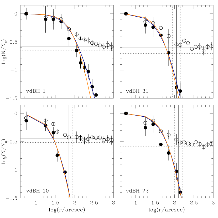
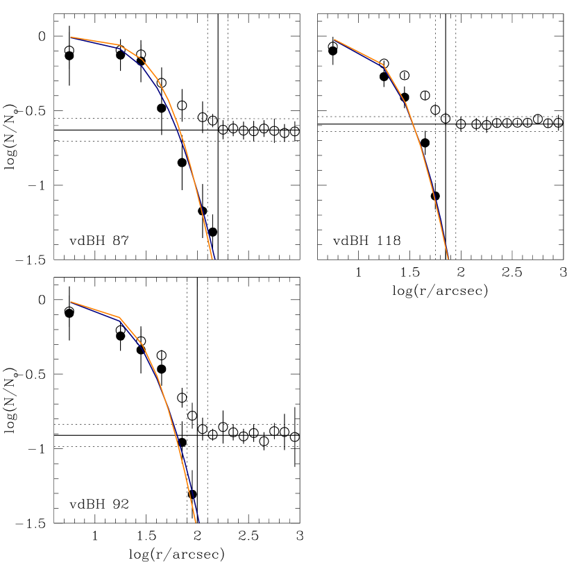
Figure 3: Stellar density profiles obtained from star counts. Open and filled circles refer to measured and background subtracted density profiles, respectively. Blue and orange solid lines depict the fitted King and Plummer curves, respectively.

The background corrected density profiles were fitted using a King (1962)’s model through the expression :

$$N\varpropto({\frac{1}{\sqrt{1+(r/r_{c})^{2}}}-\frac{1}{\sqrt{1+(r_{t}/r_{c})^{2}}}})^{2}$$ (10)

where $r_{c}$ and $r_{t}$ are the core and tidal radii, respectively (see Table 9 and Fig. 3). We used a grid of $r_{c}$ and $r_{t}$ values spanning the whole range of radii (Piskunov et al., 2007) and minimised $\chi$². The values derived for $r_{c}$ and $r_{t}$ from the fit are listed in Table 9, while the respective King’s curves are plotted with blue solid lines in Fig. 3. As can be seen, the King profiles satisfactorily reproduce the whole cluster extensions. Nevertheless, in order to get independent estimates of the star cluster half-mass radii, we fitted Plummer’s profiles using the expression:

$$N\varpropto\frac{1}{(1+(r/a)^{2})^{2}}$$ (11)

where $a$ is the Plummer’s radius, which is related to the half-mass radius ($r_{h}$) by the relation $r_{h}$ $\sim$ 1.3$a$. The resulting $r_{h}$ values are listed in Table 9 and the corresponding Plummer’s curves are drawn with orange solid lines in Fig. 3.

Table 9: Fundamental parameters of vdBH open clusters.

Star cluster	$E(B-V)$	$(m-M)_{o}$	d	$r_{c}$	$r_{h}$	$r_{cls}$	$r_{t}$	$\log(t)$	Ziso	$M_{cls}$	$t_{r}$
	(mag)	(mag)	(kpc)	(pc)	(pc)	(pc)	(pc)			(M⊙)	(Myr)
vdBH 1	0.10$\pm$0.03	13.10$\pm$0.20	4.2${}^{+0.5}_{-0.4}$	1.6$\pm$0.2	3.0$\pm$0.3	6.4${}^{+1.6}_{-1.3}$	22.4$\pm$2.0	9.10	0.0152	378$\pm$32	42.0
vdBH 10	0.60$\pm$0.10	12.50$\pm$0.20	3.2${}^{+0.3}_{-0.2}$	0.4$\pm$0.1	0.7$\pm$0.2	1.1${}^{+0.3}_{-0.2}$	2.3$\pm$0.2	7.80	0.0152	120$\pm$10	3.0
vdBH 31	0.30$\pm$0.05	12.30$\pm$0.20	2.9${}^{+0.3}_{-0.2}$	0.6$\pm$0.1	1.1$\pm$0.2	1.6${}^{+0.4}_{-0.3}$	4.9$\pm$1.4	9.10	0.0152	133$\pm$12	7.0
vdBH 72	0.85$\pm$0.10	12.60$\pm$0.30	3.3${}^{+0.5}_{-0.4}$	0.8$\pm$0.2	1.4$\pm$0.2	2.0${}^{+0.5}_{-0.4}$	4.8$\pm$0.8	8.55	0.0152	301$\pm$26	13.0
vdBH 87	0.45$\pm$0.05	11.30$\pm$0.20	1.8${}^{+0.2}_{-0.1}$	0.3$\pm$0.1	0.6$\pm$0.1	1.4${}^{+0.4}_{-0.3}$	3.5$\pm$0.9	8.50	0.0152	132$\pm$12	3.0
vdBH 92	0.35$\pm$0.05	11.50$\pm$0.20	2.0${}^{+0.2}_{-0.1}$	0.3$\pm$0.1	0.6$\pm$0.2	1.0${}^{+0.3}_{-0.2}$	2.4$\pm$0.5	8.20	0.0152	84$\pm$8	3.0
vdBH 118	0.35$\pm$0.05	14.00$\pm$0.25	6.3${}^{+0.8}_{-0.7}$	0.8$\pm$0.2	1.4$\pm$0.3	2.2${}^{+0.5}_{-0.4}$	4.6$\pm$0.9	9.45	0.0110	113$\pm$10	9.0

Note: to convert 1 arcsec to pc, we use the following expression,10$\times$10${}^{(m-M)_{o}/5}$sin(1/3600), where $(m-M)_{o}$ is the true distance modulus.

3.2 Colour-magnitude diagram analysis

3.2.1 Cleaning the cluster colour-magnitude diagrams

We used the mean cluster radii to extract the cluster colour-magnitude diagrams (CMDs). They account for the luminosity function, colour distribution and stellar density of the stars distributed along the cluster line of sights, so that we statistically cleaned the CMDs before using them to estimate the cluster fundamental parameters.

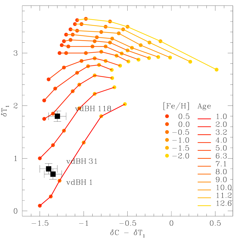
Figure 12: $\delta$$T_{1}$ versus $\delta$$C$ - $\delta$$T_{1}$ diagram with iso-age lines and iso-metallicity locii. Metallicity and age labels are given in dex and Gyr, respectively.

We employed the cleaning procedure developed by Piatti & Bica (2012, see their Fig. 12). The method compares the extracted cluster CMD to distinct CMDs composed of stars located reasonably far from the object, but not too far so as to risk losing the local field-star signature in terms of stellar density, luminosity function and/or colour distribution. Here we chose four field regions, each one designed to cover an equal area as that of the cluster, and placed around the cluster. Note that the four selected fields could not adequately represent the fore/background of the cluster if the extinction varies significantly accross the field of view.

Comparisons of field and cluster CMDs have long been done by comparing the numbers of stars counted in boxes distributed in a similar manner throughout both CMDs. However, since some parts of the CMD are more densely populated than others, counting the numbers of stars within boxes of a fixed size is not universally efficient. For instance, to deal with stochastic effects at relatively bright magnitudes (e.g., fluctuations in the numbers of bright stars), larger boxes are required, while populous CMD regions can be characterized using smaller boxes. Thus, the use of boxes of different sizes distributed in the same manner throughout both CMDs leads to a more meaningful comparison of the numbers of stars in different CMD regions. Precisely, the procedure of Piatti & Bica (2012) carries out the comparison between field-star and cluster CMDs by using boxes which vary their sizes from one place to another throughout the CMD and are centred on the positions of every star found in the field-star CMD.

By starting with reasonably large boxes – typically ($\Delta$(magnitude),$\Delta$(colour)) = (1.00, 0.50) mag – centred on each star in the four field CMDs and by subsequently reducing their sizes until they reach the stars closest to the boxes’ centres in magnitude and colour, separately, we defined boxes which result in use of larger areas in field CMD regions containing a small number of stars, and vice versa. Note that the definition of the position and size of each box involves two field stars, one at the centre of the box and another -the closest one to box centre - placed on the boundary of that box. Next, we plotted all these boxes for each field CMD on the cluster CMD and subtracted the star located closest to each box centre. Since we repeated this task for each of the four field CMD box samples, we could assign a membership probability to each star in the cluster CMD. This was done by counting the number of times a star remained unsubtracted in the four cleaned cluster CMDs and by subsequently dividing this number by four. Thus, we distinguished field populations projected on to the cluster area, i.e., those stars with a probability $P$ $\leq$ 25%; stars that could equally likely be associated with either the field or the object of interest ($P$ = 50%); and stars that are predominantly found in the cleaned cluster CMDs ($P\geq$ 75%) rather than in the field-star CMDs. Statistically speaking, a certain amount of cleaning residuals is expected, which depends on the degree of variability of the stellar density, luminosity function and colour distribution of the field stars.

Fig. 4 illustrates the performance of the cleaning procedure in the field of vdBH 72, where we plotted three different ($V$,$V-I$) CMDs: a single field-star CMD (top left-hand panel) for a circular region with an area equal to that of the cluster; that for the stars located within the cluster radius (bottom left-hand panel); and the cleaned cluster CMD (bottom right-hand panel) for stars with $P\leq$ 25% (pink), $P=$ 50% (light blue) and $P\leq$ 75% (dark blue). In the field-star CMD we overplotted the boxes generated by the cleaning procedure. A schematic finding chart with a circle of radius equal to the cluster radius is shown in the top right-hand panel.

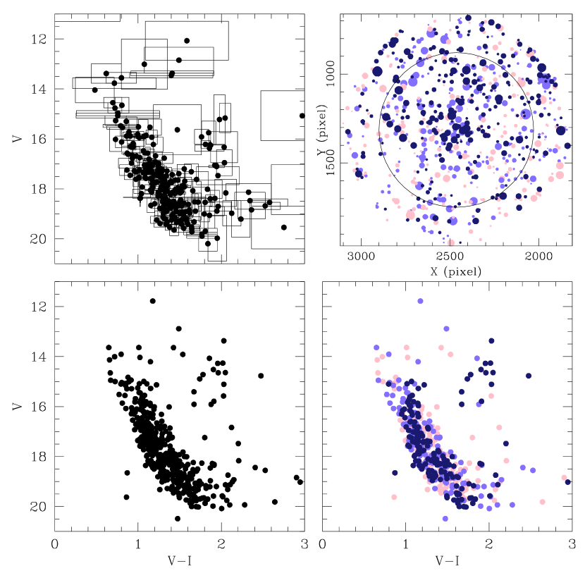
Figure 4: CMDs for stars in the field of vdBH 72: the observed CMD composed of the stars distributed within the cluster radius (bottom left-hand panel); a field CMD for a circular region placed far from the cluster and with a size equal to the cluster area (top left-hand panel), and the corresponding defined set of boxes overplotted; the cleaned cluster CMD (bottom right-hand panel). Colour-scaled symbols represent stars that statistically belong to the field ($P\leq$ 25%, pink), stars that might belong to either the field or the cluster ($P=$ 50%, light blue), and stars that predominantly populate the cluster region ($P\geq$ 75%, dark blue). The schematic finding chart for the cluster area is shown in the top right-hand panel. The black circle represents the adopted cluster radius. Symbols are as in the bottom right-hand panel, with sizes proportional to the stellar brightnesses. North is up; East is to the left.

3.2.2 Fundamental cluster parameters

Figures 5 to 11 show the whole set of CMDs and colour-colour (CC) diagrams for the cluster sample that can be exploited from the present extensive multi-band photometry. They include every magnitude and colour measurements of stars located within the respective cluster radii (see Table 9). We have also incorporated to the figures the statistical photometric memberships obtained in Sect. 3.2.1 by distinguishing stars with different colour symbols as in Fig. 4. At first glance, the cleaned cluster CMDs (stars with $P\geq$ 75%) resemble those moderately young to intermediate-age, projected on to star fields with different levels of crowdness.

Piatti & Perren (2015) introduced a new age-metallicity diagnostic diagram for the Washington photometric system, $\delta$$T_{1}$ versus $\delta$$C$ - $\delta$$T_{1}$, which has shown the ability of unambiguously providing age and metallicity estimates, simultaneously. $\delta$$C$ and $\delta$$T_{1}$ are the respective magnitude differences between the giant branch clump and the main sequence turnoff (MSTO). The new procedure allows to derive ages from 1 up to 13 Gyr and metallicities [Fe/H] from -2.0 up to +0.5 dex, and is independent of the cluster reddening and distance modulus. We used here that procedure to estimate the age and metallicity of three clusters (vdBH 1, 31 and 118) whose cleaned CMDs show a handful of red clump (RC) stars (see Figs. 5, 7 and 11), besides their MSTOs. We used the cleaned cluster CMDs to measure $C$ and $T_{1}$ magnitudes at the MSTO and RC, then computed $\delta$$C$ and $\delta$$T_{1}$ and entered into the age-metallicity diagnostic diagram to estimate cluster ages and metallicities. The resulting $\delta$$T_{1}$ and $\delta$$C$ - $\delta$$T_{1}$ values with their uncertainties are drawn in Fig. 12, where we have traced iso-age lines and marked iso-abundance positions using colour-coded lines and filled circles, respectively. From this figure we estimated by interpolation ages of 1.3$\pm$0.2 Gyr, 1.5$\pm$0.2 Gyr and 2.9$\pm$0.4 Gyr for vdBH 1, 31 and 118, respectively. As for the mean metallicities, although rather more uncertain than the ages ($\sigma$[Fe/H]= 0.25 dex), the clusters appear to be of solar or slightly subsolar metal content.

For the remaining clusters in our sample (vdBH 10, 72, 87 and 92) – whose CMDs and CC diagrams resemble those of young clusters (see Figs. 6, 8, 9 and 10) – we also adopted a solar metal content (see last column of Table 9). Note that, by considering the whole metallicity range of the Milky Way open clusters (see, e.g. Paunzen et al., 2010; Heiter et al., 2014) and by using the theoretical isochrones of Bressan et al. (2012), the differences at the zero age main sequence (ZAMS) in $V-I$ and $T_{1}-T_{2}$ colours is smaller than $\sim$ 0.08 and 0.04 mag, respectively. This result implies that negligible differences between the ZAMSs for the cluster metallicity and that of solar metal content would appear, keeping in mind the intrinsic spread of the stars in the $V$ vs $V-I$ and $T_{1}$ vs $T_{1}-T_{2}$ CMDs.

The availability of six CMDs and three different CC diagrams covering wavelengths from the blue up to the near-infrarred allowed us to derive reliable ages, reddenings and distances for the studied clusters. Particularly noticeable in the $V$ vs $U-B$ CMD, but applicable to every CMD, the shape of the main sequence (MS), its curvatures (those less and more pronounced), the relative distance between the RC and the MSTO in magnitude and colour separately, among others, are features tightly related to the cluster age, regardless their reddenings and distances. For this reason, we started by selecting theoretical isochrones (Bressan et al., 2012) with the adopted cluster metallicities in order to chose those which best match the clusters’ features in the CMDs. From our first choices, we derived the cluster reddenings by shifting those isochrones in the three CC diagrams following the reddening vectors until their bluest points coincided with the observed ones. Note that this requirement allowed us to use the $V-R$ vs $R-I$ CC diagram as well, even though the reddening vector runs almost parallell to the cluster sequence. Finally, the mean $E(B-V)$ colour excesses were used to properly shift the chosen isochrones in the CMDs in order to derive the cluster true distance modulii by shifting the isochrones along the magnitude axes.

We iterated this procedure whenever refinements in the cluster ages were necessary. Nevertheless, we found that isochrones bracketing the initial age choice by $\Delta$ log($t$ yr^-1) = $\pm$0.10 represent the overall age uncertainties owing to the observed dispersion in the cluster CMDs and CC diagrams. Although in some cases the age dispersion is smaller than $\Delta$ log($t$ yr^-1) = 0.10, we prefer to keep the former value as an upper limit to our error budget. In order to enter the isochrones into the CMDs and CC diagrams we used the following ratios: $E(U-B)$/$E(B-V)$ = 0.72 + 0.05$\times$$E(B-V)$ (Hiltner & Johnson, 1956); $E(V-R)$/$E(B-V)$ = 0.65, $E(V-I)$/$E(B-V)$ = 1.25, $A_{V}$/$E(B-V)$ = 3.1 (Cardelli et al., 1989); $E(C-T_{1})$/$E(B-V)$ = 1.97, $E(T_{1}-T_{2})$/$E(B-V)$ = 0.692, $A_{T_{1}}$/$E(B-V)$ = 2.62 (Geisler, 1996). The adopted best matched isochrones are overplotted on Figs. 5 to 11, while the resulting values with their errors for the cluster reddenings, true distance modulii and ages are listed in Table 9.

The masses of the clusters in our sample were derived by summing the individual masses of stars with membership probabilities $P\geq$ 75%. The latter were obtained by interpolation in the theoretical isochrones traced in Figs. 5 to 11 from the observed $V$ magnitude of each star, properly corrected by reddening and distance modulus. We estimate the uncertainty in the mass to be $\sigma(\log(M_{cls}/\hbox{M${}_{\odot}$}))$ $\sim$ 0.2 dex. Note that this error comes from propagation of the $V$ magnitude errors in the mass distribution along the theoretical isochrones. It does not reflect the deviation of the cluster mass computed from stars with $P\geq$ 75% from the actual total cluster mass. Nevertheless, at first glance, the appearance of the cluster CMDs and CC diagrams ($P\geq$ 75%) do not seem to significantly differ from those including any other observed stars placed along the adopted isochrones with $P<$ 75%, thought to be cluster stars. At the same time, the computed cluster masses include some unavoidable interlopers, which mitigate the loss of some cluster stars. In the case of vdBH 118, the derived mass should be considered as a very lower limit, since its CMDs barely reach the cluster MSTO. For the remaining clusters, our photometry reach well below the fainter MS cluster stars. Using the resulting masses and the half-mass radii $r_{h}$ of Table 9, we computed the half-mass relaxation times using the equation (Spitzer & Hart, 1971):

$$t_{r}=\frac{8.9\times 10^{5}M_{cls}^{1/2}r_{h}^{3/2}}{\bar{m}log_{10}(0.4M_{cls}/\bar{m})},$$ (12)

where $M_{cls}$ is the cluster mass and $\bar{m}$ is the mean mass of the cluster stars. The derived masses and relaxation times are listed in Table 9. If we considered non-oberved stars with masses between 1 and 0.5 M_⊙ and the Salpeter’s mass function, the relaxation times would increase in $\sim$ 10 per cent.

4 results and discussion

vdBH 10 (= Ruprecht 35) and 31 (= Ruprecht 60) have age estimates of 400$\pm$100 Myr derived from Two-Micron All-Sky Survey (2MASS) photometry (Bonatto & Bica, 2010), which clearly differs from our values (see Table 9). By inspecting their 2MASS $J$ vs $J-H$ CMDs (Figures 4 and 5 in Bonatto & Bica (2010)), and considering the relationship $M_{J}$ vs $M_{V}$ for the cluster ages computed by Bressan et al. (2012) and our cluster distances, we found that the faintest reached $J$ magnitude ($\approx$ 15.5 mag) corresponds to $V$ $\approx$ 16.3 mag and 16.6 mag for vdBH 10 and 31, respectively. This suggests that the used 2MASS photometry is shallower than the present one. On the other hand, we speculate with the possibility that the field-star cleaning procedure applied by Bonatto & Bica (2010) have left significant residuals (see Piatti & Bica, 2012; Han et al., 2016); thus leading them to derive ages which reflect the composite stellar population along the cluster line-of-sights. Curiously, both clusters have nearly similar angular Galactic coordinates. Additionally, the 2MASS CMDs were extracted using sky areas much larger than those embracing the clusters, so that field-stars can quantitatively prevail over cluster stars. For these reasons, we are confidence of the present multi-band photometry and resulting cluster parameters.

The distance modulus and age of vdBH 10 (= Ruprecht 35) were previously estimated by Moitinho et al. (2006) and soon after used by Vázquez et al. (2008) in an updated study of the spiral structure of the outer Galactic disc. Moitinho et al. (2006) estimated a distance from the Sun of 5.32 kpc and an age of 70 Myr. While the cluster age is in excellent agreement with the present value, the cluster distance differs significantly. This could be due either to a photometric zero point offset or to the use of field star contaminated CMD diagrams in the analysis carried out by Moitinho et al. (2006). Both sources of error have been checked within our photometric data set. On the one hand, we used six different CMDs involving $V$ and $T_{1}$ magnitudes, as well as $U-B$, $B-V$, $V-R$, $R-I$, $C-T_{1}$ and $T_{1}-T_{2}$ colours. On the other hand, we have had particular care in cleaning the cluster CMDs from field star contamination (Sect. 3.2.1). As fas as we are aware, we are confident of the realibility of the present cluster distance.

vdBH 31 (= Ruprecht 60) was more recently studied by Carraro et al. (2013) using $UBVI$ photometry. The authors mentioned that their photometry does not cover the object completely and that they did not perform any cleaning of field stars in the cluster CMD. They estimated an age of $\sim$1.5 Gyr, a metallicity of [Fe/H] $\sim$ -0.5 dex, an $E(B-V)$ colour excess of 0.13$\pm$0.10 mag and a distance from the Sun of 4.5 kpc. Their age, reddening and distance are in very good agreement with our values. As for the remarkable low metal abundance, our metallicity sensitive Washington $C$ photometry do not support such a low value. Carraro et al. (2013) could have included field stars in their CMD which, alongside the fewer cluster stars measured, could lead to such a low value.

Finally, Giorgi et al. (2015) studied vdBH 31 (= Ruprecht 60) also from $UBVI$ photometry. They derived $E(B-V)$ = 0.37$\pm$0.05 mag, a distance from the Sun of 4.2$\pm$0.2 kpc and an age of 0.8-1.0 Gyr. While the estimated reddening is in faily good agreeement with our value, they derived a slightly younger age which in turn led to estimate a larger distance. We are confident of our age value which comes from a CMD analysis as well as from the Washington age-metallicity diagnostic diagram analysis.

We computed Galactic coordinates using the derived cluster heliocentric distances, their angular Galactic coordinates and a Galactocentric distance of the Sun of R${}_{GC_{\odot}}$ = 8.3 kpc (Hou & Han, 2014, and references therein). The resulting spatial distribution is depicted in Fig. 13, where we added for comparison purposes the 2167 open clusters catalogued by Dias et al. (2002, version 3.5 as of January 2016) and the schematic positions of the spiral arms (Drimmel & Spergel, 2001; Moitinho et al., 2006). The studied clusters are mostly located between the Carina and Perseus arms, with the sole exception of vdBH 118, which lies between the Carina and Crux spiral arms and is one of the most distant open clusters from the Sun in that direction as well. In general terms, the seven vdBH clusters are distributed outside the circle around the Sun (d $\sim$ 2.0 kpc) where the catalogued clusters are mostly concentrated.

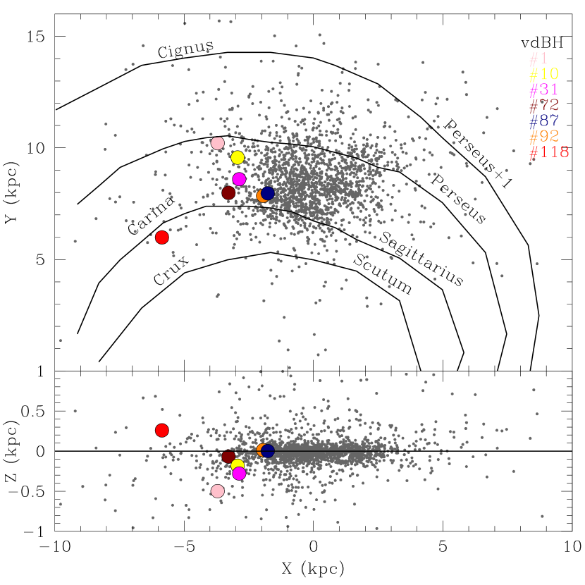
Figure 13: Galactic spatial distribution of the studied clusters. Open clusters from the catalogue of Dias et al. (2002, version 3.5 as of January 2016) are drawn with gray dots, while the schematic positions of spiral arms (Drimmel & Spergel, 2001; Moitinho et al., 2006) are traced with black solid lines.

The structural parameters estimated from the stellar density radial profiles in combination with the fundamental properties derived from the analysis of CMDs and CC diagrams allow us to investigate the internal dynamical state of the clusters. Here we consider the effect of the internal dynamical evolution (two-body relaxation, mass segregation, etc). As for the Galactic tidal field, bearing in mind the Galactocentric distances of the studied clusters (R_GC $\approx$ 8.1$-$10.9 kpc, with a mean value of 9$\pm$1 kpc) and their ages (see Table 9), the differences in the potential will lead to $\sim$ 10 per cent variations in the half mass radius (Miholics et al., 2014, see, e.g., their figures 1).

The age/$t_{r}$ ratio is a good indicator of the internal dynamical evolution, since it gives the number of times the characteristic time-scale to reach some level of energy equipartition (Binney & Merrifield, 1998) has been surpassed. Star clusters with large age/$t_{r}$ ratios have reached a higher degree of relaxation and hence are dynamically more evolved. As Fig. 14 shows, our clusters appear to cover a wide range of age/$t_{r}$ ratios, from $\sim$ 20 up to 320, all of them suggesting that the clusters have had enough time to evolve dynamically. In the figure we included in grey colour 236 open clusters analysed by Piskunov et al. (2007), who derived from them homogeneous scales of radii and masses. They derived core and tidal radii for their cluster sample, from which we calculated the half-mass radii and, with their clusters masses and eq. 12, relaxation times, by assuming that the cluster stellar density profiles can be indistinguishably reproduced by King and Plummer models. Their cluster sample are mostly distributed inside a circle of $\sim$ 1 kpc from the Sun. As can be seen, our clusters cover the most evolved limit of the age/$t_{r}$ distribution (right-hand panels).

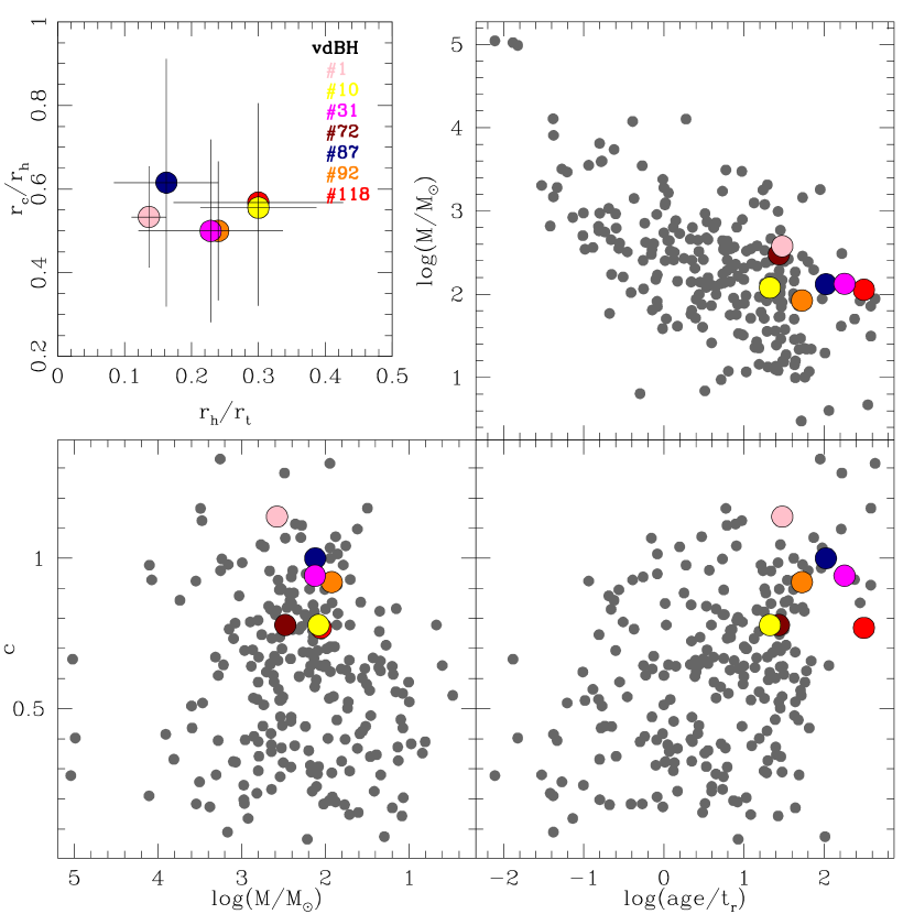
Figure 14: Relationships between cluster core ($r_{c}$), half-mass ($r_{h}$) and tidal ($r_{t}$) radii, concentration parameter ($c$), mass, age and relaxation time ($t_{r}$).

Grey dots correspond to 236 star clusters with homogeneous estimations of masses and radii derived by Piskunov et al. (2007).

Since dynamical evolution implies the loss of stars (mass loss), we expect some trend of the present-day cluster mass with the age/$t_{r}$ ratio. This is confirmed in the top-right panel of Fig. 14, where the larger the present-day mass the less the dynamical evolution of a cluster in the solar neighbourhood, with a noticeable scatter. The studied clusters appear to have relatively large masses for their particular internal dynamical states. Curiously, selection against poor and old clusters could suggest the beggining of cluster dissolution, with some exceptions.

Trenti et al. (2010) presented a unified picture for the evolution of star clusters on the two-body relaxation timescale from direct N-body simulations of star clusters in a tidal field. Their treatment of the stellar evolution is based on the approximation that most of the relevant stellar evolution occurs on a timescale shorter than a relaxation time, when the most massive stars lose a significant fraction of mass and consequently contribute to a global expansion of the system. Later in the life of a star cluster, two-body relaxation tends to erase the memory of the initial density profile and concentration. They found that the structure of the system, as measured by the core to half mass radius ratio, the concentration parameter $c$= log($r_{t}/r_{c}$), among others, evolve toward a universal state, which is set by the efficiency of heating on the visible population of stars induced by dynamical interactions in the core of the system. In the bottom panels of Fig. 14 we plotted the dependence of the concentration parameter $c$ with the cluster mass and the age/$t_{r}$ ratio, respectively. They show that our dynamically evolved clusters are within those with relatively high $c$ values, and that star clusters tend to initially start their dynamical evolution with relatively small concentration parameters. Likewise, star clusters in an advanced dynamical state can also have relatively lower $c$ values due to their smaller masses.

According to Heggie & Hut (2003, see, e.g., their figure 33.2) a star cluster dynamically evolving with its tidal radius filled, moves in the $r_{c}/r_{h}$ vs $r_{h}/r_{t}$ plane parallel to the $r_{c}/r_{h}$ axis ($r_{h}/r_{t}$ $\sim$ 0.21) toward low values due to violent relaxation in the cluster core region followed by two-body relaxation, mass segregation, and finally core-collapse. Top-left panel in Fig. 14 shows that the studied clusters have $r_{h}/r_{t}$ ratios in fairly agreement, within the uncertainties, with that of tidally filled clusters, and $r_{c}/r_{h}$ ratios suggesting mass segregation in their core regions.

We finally built the cluster mass functions (MFs) employing the masses of stars with photometric memberships $P\geq$ 75%. The resulting MFs are shown in Fig. 15 where the errorbars come from applying Poisson statistics. We did not include vdBH 118 because of incompleteness in our photometry for its MS. For comparison porpuses we superimposed the relationship given by Salpeter (1955, slope = -2.35) for the stars in the solar neighbourhood. As can be seen, despite their advanced state of dynamical evolution, vdBH 1, 72 and 87 still keep their MFs close to that of Salpeter’s law, while the remaining clusters (vdBH 10, 31 and 92) show MFs which depart from it for smaller masses toward a relation with a smaller slope (see, e.g. Lim et al., 2015; Santos et al., 2016). Their total masses, structural parameters and age/$t_{r}$ ratios do not suggest any hint to explain such differences, and prevent us to draw any conclusion from such a small cluster sample.

Figure 15: Mass function for clusters in our sample. The Salpeter (1955)’ relationship for stars in the solar neighbourhood is superimposed.

5 conclusions

We present results of seven star clusters identified by van den Bergh & Hagen (1975), namely, vdBH 1, 10, 31, 72, 87, 92, and 118, for which particular attention was not given until now. The clusters were observed through the Johnson $UBV$, Kron-Cousins $RI$ and Washington $C$ filters; four of them (vdBH 72, 87, 92 and 118) are photometrically study for the first time.

The multi-band photometric data sets were used to trace the cluster stellar density radial profiles and to build CMDs and CC diagrams, from which we estimate their structural parameters and fundamental astrophysical properties. Their radial profiles were built from star counts carried out throughout the observed fields using the final photometric catalogues. We derived the cluster radii from a careful placement of the background levels and fitted King and Plummer models to derive cluster core, half-mass and tidal radii. We then applied a subtraction procedure developed by Piatti & Bica (2012) to statistically clean the star cluster CMDs and CC diagrams from field star contamination in order to disentangle star cluster features from those belonging to their surrounding fields. The employed technique makes use of variable cells in order to reproduce the field CMD as closely as possible.

The availability of three CC diagrams and six CMDs covering wavelengths from the blue up to the near-infrarred allowed us to derive reliable ages, reddenings and distances for the studied clusters. We exploited such a wealth in combination with a new age-metallicity diagnostic diagram for the Washington system and theoretical isochrones computed by Bressan et al. (2012) to find out that the clusters in our sample cover a wide age range, from $\sim$ 60 Myr up to 2.8 Gyr, are of relatively small size ($\sim$ 1 $-$ 6 pc) and are placed at distances from the Sun which vary between 1.8 and 6.3 kpc, respectively. They are located between the Carina and Perseus spiral arms, with the exception of vdBH 118, which is closer to the Galactic centre than the Carina arm. It also belongs to the sample of the farthest known clusters placed between the Carina and Crux spiral arms.

We estimated lower limits for the cluster present-day masses as well as half-mass relataxion times. Their resulting values suggest that the studied clusters have advanced states of their internal dynamical evolution, i.e., their ages are many times the relaxation times ($\sim$ 20 $-$ 320). When combined with the obtained structural parameters, we found that the clusters are possible in the phase typical of those tidally filled with mass segregation in their core regions.

We compared the cluster masses, concentration parameters and age/$t_{r}$ ratios with those for 236 clusters located in the solar neighbourhood. The seven vdBH clusters are within more massive ($\sim$ 80 $-$ 380M_⊙), with higher $c$ values, and dynamically evolved ones. There is also a broad correlation between the cluster massses and the dynamical state, in the sense that the more the advanced the internal dynamical evolution, the less the cluster mass. The apparent decrease of clusters with masses smaller than $\sim$ 200M_⊙ and ages $\sim$ 100 times older than their relaxation times could suggest the beggining of cluster dissolution, with some exceptions. Finally, we found that the MFs of vdBH 1, 72 and 87 follow approximately the Salpeter (1955)’s relationship, while vdBH 10, 31 and 92 seem to show shallower MFs for the lower mass regime.

Figure 5: CMDs and CC diagrams for stars measured in the field of vdBH 1. Symbols are as in Fig. 4. We overplotted the isochrone which best matches the cluster features (see text for details).

Figure 6: CMDs and CC diagrams for stars measured in the field of vdBH 10. Symbols are as in Fig. 4. We overplotted the isochrone which best matches the cluster features (see text for details).

Figure 7: CMDs and CC diagrams for stars measured in the field of vdBH 31. Symbols are as in Fig. 4. We overplotted the isochrone which best matches the cluster features (see text for details).

Figure 8: CMDs and CC diagrams for stars measured in the field of vdBH 72. Symbols are as in Fig. 4. We overplotted the isochrone which best matches the cluster features (see text for details).

Figure 9: CMDs and CC diagrams for stars measured in the field of vdBH 87. Symbols are as in Fig. 4. We overplotted the isochrone which best matches the cluster features (see text for details).

Figure 10: CMDs and CC diagrams for stars measured in the field of vdBH 92. Symbols are as in Fig. 4. We overplotted the isochrone which best matches the cluster features (see text for details).

Figure 11: CMDs and CC diagrams for stars measured in the field of vdBH 118. Symbols are as in Fig. 4. We overplotted the isochrone which best matches the cluster features (see text for details).

References

- Binney & Merrifield (1998) Binney J., Merrifield M., 1998, Galactic Astronomy
- Bonatto & Bica (2010) Bonatto C., Bica E., 2010, MNRAS, 407, 1728
- Bressan et al. (2012) Bressan A., Marigo P., Girardi L., Salasnich B., Dal Cero C., Rubele S., Nanni A., 2012, MNRAS, 427, 127
- Cardelli et al. (1989) Cardelli J. A., Clayton G. C., Mathis J. S., 1989, ApJ, 345, 245
- Carraro et al. (2013) Carraro G., Beletsky Y., Marconi G., 2013, MNRAS, 428, 502
- Dias et al. (2002) Dias W. S., Alessi B. S., Moitinho A., Lépine J. R. D., 2002, A&A, 389, 871
- Drimmel & Spergel (2001) Drimmel R., Spergel D. N., 2001, ApJ, 556, 181
- Geisler (1996) Geisler D., 1996, AJ, 111, 480
- Giorgi et al. (2015) Giorgi E. E., Solivella G. R., Perren G. I., Vázquez R. A., 2015, New Astron., 40, 87
- Han et al. (2016) Han E., Curtis J. L., Wright J. T., 2016, preprint, (arXiv:1605.05330)
- Heggie & Hut (2003) Heggie D., Hut P., 2003, The Gravitational Million-Body Problem: A Multidisciplinary Approach to Star Cluster Dynamics
- Heiter et al. (2014) Heiter U., Soubiran C., Netopil M., Paunzen E., 2014, A&A, 561, A93
- Hiltner & Johnson (1956) Hiltner W. A., Johnson H. L., 1956, ApJ, 124, 367
- Hou & Han (2014) Hou L. G., Han J. L., 2014, A&A, 569, A125
- King (1962) King I., 1962, AJ, 67, 471
- Landolt (1992) Landolt A. U., 1992, AJ, 104, 340
- Lim et al. (2015) Lim B., Sung H., Hur H., Park B.-G., 2015, preprint, (arXiv:1511.01118)
- Miholics et al. (2014) Miholics M., Webb J. J., Sills A., 2014, MNRAS, 445, 2872
- Moitinho et al. (2006) Moitinho A., Vázquez R. A., Carraro G., Baume G., Giorgi E. E., Lyra W., 2006, MNRAS, 368, L77
- Paunzen et al. (2010) Paunzen E., Heiter U., Netopil M., Soubiran C., 2010, A&A, 517, A32
- Piatti & Bica (2012) Piatti A. E., Bica E., 2012, MNRAS, 425, 3085
- Piatti & Perren (2015) Piatti A. E., Perren G. I., 2015, MNRAS, 450, 3771
- Piskunov et al. (2007) Piskunov A. E., Schilbach E., Kharchenko N. V., Röser S., Scholz R.-D., 2007, A&A, 468, 151
- Salpeter (1955) Salpeter E. E., 1955, ApJ, 121, 161
- Santos et al. (2016) Santos Jr. J. F. C., Roman-Lopes A., Carrasco E. R., Maia F. F. S., Neichel B., 2016, MNRAS, 456, 2126
- Skrutskie et al. (2006) Skrutskie M. F., et al., 2006, AJ, 131, 1163
- Spitzer & Hart (1971) Spitzer Jr. L., Hart M. H., 1971, ApJ, 164, 399
- Stetson et al. (1990) Stetson P. B., Davis L. E., Crabtree D. R., 1990, in Jacoby G. H., ed., Astronomical Society of the Pacific Conference Series Vol. 8, CCDs in astronomy. pp 289–304
- Trenti et al. (2010) Trenti M., Vesperini E., Pasquato M., 2010, ApJ, 708, 1598
- Vázquez et al. (2008) Vázquez R. A., May J., Carraro G., Bronfman L., Moitinho A., Baume G., 2008, ApJ, 672, 930