A Note on Computable Proximity of $\mathcal{L}_{1}$-Discs
on the Digital Plane

Abstract.

This paper investigates problems in the characterization of the proximity of digital discs. Based on the $\mathcal{L}_{1}$-metric structure for the 2D digital plane and using a Jaccard-like metric, we determine numerical characters for intersecting digital discs.

1. Introduction

This paper introduces a form of digital geometry in proximity spaces. The study of digital discs is connected to the discovery of proximal objects [13, 12, 3]. The objects often can be represented as sets of points and this stipulates that set-theoretic and topological methods are very useful tools in the study of proximity relations. Digital geometry deals with geometric properties of objects on computer screens [7, 8, 9, 14].

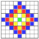
Figure 1. Structures

Many different computer screen images can be obtained via pixel lighting. A pixel is the smallest element is a digital image and are usually identified as points. In other words, we can describe images on the computer screen by their pixels that have digital valued coordinates, i.e., a mathematical model of the computer screen is the digital plane $\mathbb{Z}^{2}$.

The importance of the notions of the circle and disc in Euclidean geometry is well known. In digital geometry, digital circles and digital discs have various important properties that are different from the Euclidean ones (see, e.g., [11, 10, 6, 16, 1]). One of the reasonable realizations of metric structure on the digital plane $\mathbb{Z}^{2}$ can be determined via the so-called $\mathcal{L}_{1}$ metric. This metric has the following view:

$$d\left(p_{1},p_{2}\right)=\lvert a_{1}-a_{2}\rvert+\lvert b_{1}-b_{2}\rvert,\mbox{where $p_{1}$ and $p_{2}$ are some matched points},$$

i.e., $p_{1}$ and $p_{2}$ are pixels for our future considerations. Since we can represent pixel coordinates as digital pairs, then it is obvious that $d\left(p_{1},p_{2}\right)\in\mathbb{Z}$ (the integers).

Based on the $\mathcal{L}_{1}$ metric, we define a digital circle with radius $r$ and center $x$ (denoted by $C_{d}(x,r)$) as follows:

$$C_{d}(x,r)=\left\{z\in\mathbb{Z}^{2}:d(x,z)=r\right\}.$$

Moreover, we denote by $c\left(C_{d}(x,r)\right)$ the circumference of the circle $C_{d}(x,r)$ where $r\in\mathbb{N}\cup\left\{0\right\}$.

Due to R. Klette and A. Rosenfeld [7], it is known that $\pi_{\mathcal{L}_{1}}=\frac{c\left(C_{d}(x,r)\right)}{\mbox{diam}\left(C_{d}(x,r)\right)}=\frac{8r}{2r}=4$, where $\mbox{diam}\left(C_{d}(x,r)\right)$ is the diameter of the circle $C_{d}(x,r)$. Using this fact, we easily obtain the following result.

Lemma 1.

Let $C_{d}(x,r)$ be a digital circle with center at point $x$ and radius $r$ relative to the $\mathcal{L}_{1}$ metric. Then, for the number of pixels of $C_{d}(x,r)$, we have the formula

$$\mbox{card}\left(C_{d}(x,r)\right)=\frac{2c\left(C_{d}(x,r)\right)}{\pi_{\mathcal{L}_{1}}}=4r.$$

Fig. 1 demonstrates the structural property of the digital disc, namely,

$$D_{d}\left(x,R\right) =\left\{z\in\mathbb{Z}^{2}\mid d(x,z)\leq R\right\},\ \mbox{particularly:}$$

$$D_{d}\left(x,R\right) =\left\{x\right\}\cup\left(\mathop{\bigcup}\limits_{r=1}^{R}C_{d}(x,r)\right),\ \mbox{where}\ R\in\mathbb{Z}.$$

Lemma 2.

If $D_{d}\left(x,R\right)$ is a digital disc relative to the $\mathcal{L}_{1}$ metric $d$, then the number of pixels forming the disc $D_{d}\left(x,R\right)$ can be computed by the formula $\mbox{card}\left(D_{d}\left(x,R\right)\right)=2R^{2}+2R+1$.

Proof.

Since $D_{d}\left(x,R\right)=\left\{x\right\}\cup\left(\mathop{\bigcup}\limits_{r=1}^{R}C_{d}(x,r)\right)$, we can write

$$\mbox{card}\left(D_{d}\left(x,R\right)\right)=1+\mbox{card}\left(C_{d}(x,1)\right)+\mbox{card}\left(C_{d}(x,2)\right)+\cdots+\mbox{card}\left(C_{d}(x,R)\right).$$

Now, applying Lemma 1, we get

$$\mbox{card}\left(D_{d}\left(x,R\right)\right) =1+4+8+\cdots+4R=$$

$$=1+4\left(\frac{1+R}{2}R\right)=$$

$$=2R^{2}+2R+1.$$

∎

2. How Near are Digital Discs?

To solve a wide class of the problems of computational proximity, we know that the Hausdorff metric is appropriate [7, 2]. The Hausdroff metric (denoted by $d_{H}(A,B)$) measures the distance between the sets $A,B$ in the given metric space $(X,d)$ and is defined by

$$d_{H}(A,B)=\mbox{max}\left\{\mathop{\mbox{sup}}\limits_{x\in A}\mathop{\mbox{inf}}\limits_{y\in B}d(x,y),\mathop{\mbox{sup}}\limits_{y\in B}\mathop{\mbox{inf}}\limits_{x\in A}d(x,y)\right\}.$$

If the sets $A,B$ are finite, we obtain the simplication of the Hausdorff metric by maxima and minima [4], i.e.,

$$d_{H}(A,B)=\mbox{max}\left\{\mathop{\mbox{max}}\limits_{x\in A}\mathop{\mbox{min}}\limits_{y\in B}d(x,y),\mathop{\mbox{max}}\limits_{y\in B}\mathop{\mbox{min}}\limits_{x\in A}d(x,y)\right\}.$$

For intersecting sets $A$ and $B$, i.e., $A\cap B\neq\emptyset$, the Hausdorff metric guarantees that $d_{H}(A,B)=0$. Such sets in the theory of proximity spaces [4, §8.4] are said to be trivially near. Therefore, if $A\cap B\neq\emptyset$ and $A\cap C\neq\emptyset$ hold in the metric space $(X,d)$, we cannot distinguish which the sets in the pair $B,C$ is more near to $A$. Hence, the application of Hausdorff distance in the sorting of near sets is more suitable for disjoint sets.

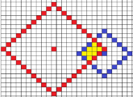
Figure 2. Overlap

Classification of images in computer science frequently need the application of Jaccard-like metrics [5]. We will use a simplified version to analyze proximity of intersecting digital discs. It must be especially noticed that the problem connected with the intersection of plane discs was considered from a computer science perspective in [15].

For the Jaccard-like metric $m$, we understand the distance function defined via the cardinality of the symmetric difference of two arbitrary nonempty finite sets $A$ and $B$, i.e.,

$$m(A,B) =\mbox{card}\left(A\bigtriangleup B\right)$$

$$=\mbox{card}\left(A\setminus B\right)+\mbox{card}\left(B\setminus A\right)$$

$$=\mbox{card}\left(A\right)+\mbox{card}\left(B\right)-2\mbox{card}\left(A\cap B\right).$$

It is obvious that if $\mbox{card}\left(A\right)\neq\mbox{card}\left(B\right)$ and both sets are finite while $A\cap B\neq\emptyset$, we get $m(A,B)\neq 0$. This raises the question of the computation of the proximity of intersecting digital discs such as the ones in Fig. 2.

Theorem 1.

Let $D_{d}(x,R_{1})$ and $D_{d}(y,R_{2})$ be digital discs such that $C_{d}(x,R_{1})\cap C_{d}(y,R_{2})\neq\emptyset$. Then

$$m\left(D_{d}(x,R_{1}),D_{d}(y,R_{2})\right)=2\left(R_{1}^{2}+R_{2}^{2}+R_{1}+R_{2}-2kn+k+n\right),$$

where $k$ and $n$ denote the number of pixels forming the width and height of the greatest rectangle subset of an intersection set.

Proof.

Appling Lemma 2, we obtain the following cardinal equalities:

$$m\left(D_{d}(x,R_{1}),D_{d}(y,R_{2})\right) =\mbox{card}\left(D_{d}(x,R_{1})\right)+\mbox{card}\left(D_{d}(y,R_{2})\right)-2\mbox{card}\left(D_{d}(x,R_{1})\cap D_{d}(y,R_{2})\right)$$

$$=2\left(R_{1}^{2}+R_{2}^{2}+R_{1}+R_{2}+1)\right)-2\mbox{card}\left(D_{d}(x,R_{1})\cap D_{d}(y,R_{2})\right)$$

$$=2\left(R_{1}^{2}+R_{2}^{2}+R_{1}+R_{2}+1\right)-2\left[kn+(k-1)(n-1)\right]$$

$$=2\left(R_{1}^{2}+R_{2}^{2}+R_{1}+R_{2}-2kn+k+n\right)$$

∎

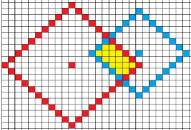
Figure 3. Non-Intersecting Boundaries

Notice that there is a situation in which two digital discs are intersecting but their boundaries are not intersecting (see, e.g., Fig.3). Observe that in that case, we have $C_{d}\left(x,R_{1}-1\right)\cap C_{d}\left(y,R_{2}\right)\neq\emptyset$, or, equivalently, $C_{d}\left(x,R_{1}\right)\cap C_{d}\left(y,R_{2}-1\right)\neq\emptyset$.

Theorem 2.

Let $D_{d}\left(x,R_{1}\right)$ and $D_{d}\left(y,R_{2}\right)$ be digital discs such that $C_{d}\left(x,R_{1}\right)\cap C_{d}\left(y,R_{2}\right)=\emptyset$, but $C_{d}\left(x,R_{1}-1\right)\cap C_{d}\left(y,R_{2}\right)\neq\emptyset$. Then we have $\mbox{m}\left(D_{d}\left(x,R_{1}\right),D_{d}\left(y,R_{2}\right)\right)=2\left(R_{1}^{2}+R_{2}^{2}+R_{1}+R_{2}+1-2kn\right)$, where $k$ and $n$ denote the number of pixels forming the width and height of the greatest rectangle subset of an intersection set.

Proof.

In this case, we can easily not that $\mbox{card}\left(D_{d}\left(x,R_{1}\right)\cap D_{d}\left(y,R_{2}\right)\right)=2kn$. Hence, we have $\mbox{m}\left(D_{d}\left(x,R_{1}\right),D_{d}\left(y,R_{2}\right)\right)=2\left(R_{1}^{2}+R_{2}^{2}+R_{1}+R_{2}+1-2kn\right)$. ∎

Next, we need to represent the centers $x$ and $y$ of discs $D_{d}\left(x,R_{1}\right)$ and $D_{d}\left(y,R_{2}\right)$ by a couple of digital coordinates as follows: $x=\left(\alpha,\beta\right)$ and $y=\left(\gamma,\delta\right)$. If one of the following equalities hold $d(x,y)=\lvert\alpha-\gamma\rvert$ or $d(x,y)=\lvert\beta-\delta\rvert$, i.e., the centers of the discs lie on horizontal or verical axes (similar to the situations shown in Fig. 4.1 and Fig. 4.2), then we can measure the proximity of the discs via computation of the pixel cardinality of the intersections sets.

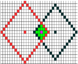
4.1 Intersecting Discs with Intersecting Boundaries

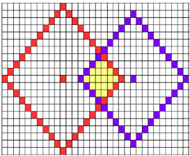
4.2 Intersecting Discs with Non-Intersecting Boundaries

Figure 4. Intersecting Discs on the Digital Plane

Theorem 3.

Let $D_{d}\left(x,R_{1}\right)$ and $D_{d}\left(y,R_{2}\right)$ be digital discs such that $x=\left(\alpha,0\right)$ and $y=\left(\gamma,0\right)$ with $\alpha<\gamma$ and $\gamma-\alpha\leq R_{1}+R_{2}$. If $C_{d}\left(x,R_{1}\right)\cap C_{d}\left(y,R_{2}\right)\neq\emptyset$, then

$$\mbox{m}\left(D_{d}\left(x,R_{1}\right),D_{d}\left(y,R_{2}\right)\right)=\left(R_{1}-R_{2}\right)^{2}+2\left(R_{1}+R_{2}+1\right)\left(\gamma-\alpha\right)-\left(\gamma-\alpha\right)^{2}.$$

Proof.

Since $x=\left(\alpha,0\right)$, $y=\left(\gamma,0\right)$ and $C_{d}\left(x,R_{1}\right)\cap C_{d}\left(y,R_{2}\right)\neq\emptyset$, we claim that

$$C_{d}\left(x,R_{1}\right)\cap C_{d}\left(y,R_{2}\right)=C_{d}(k,r),\ \mbox{where},$$

$k=\left(\frac{\alpha+R_{1}+\gamma-R_{2}}{2},0\right)$ and
$r=R_{1}-(k-\alpha)=\frac{R_{1}+R_{2}+(\gamma-\alpha)}{2}\in\mathbb{N}\cup\left\{0\right\}$. Consequently, simplification of

$$\mbox{m}\left(D_{d}\left(x,R_{1}\right),D_{d}\left(y,R_{2}\right)\right)=2\left(R_{1}^{2}+R_{2}^{2}+R_{1}+R_{2}+1-2r^{2}-2r-1\right)$$

gives the needed expression

$$\mbox{m}\left(D_{d}\left(x,R_{1}\right),D_{d}\left(y,R_{2}\right)\right)=\left(R_{1}-R_{2}\right)^{2}+2\left(R_{1}+R_{2}+1\right)\left(\gamma-\alpha\right)-\left(\gamma-\alpha\right)^{2}.$$

∎

Observe that Theorem 3 can be applied in similar cases when the intersection set of the digital discs itself is a disc.

This leads us to consider two intersecting digital discs with non-intersecting boundaries (see, e.g., Fig. 4.2) so that both centers lie on the horizontal or vertical axes. In such cases, we obtain the following result.

Corollary 1.

Let $D_{d}\left(x,R_{1}\right)$ and $D_{d}\left(y,R_{2}\right)$ be intersecting digital discs that satisfy the conditions of Theorem 3, but $C_{d}\left(x,R_{1}\right)\cap C_{d}\left(y,R_{2}\right)=\emptyset$. Then we have

$$\mbox{m}\left(D_{d}\left(x,R_{1}\right),D_{d}\left(y,R_{2}\right)\right) =2\left(R_{1}^{2}+R_{2}^{2}+R_{1}+R_{2}-2r_{0}^{2}-4r_{0}+1\right),\mbox{where},$$

$$r_{0} =\frac{R_{1}-1+R_{2}+(\gamma-\alpha)}{2}.$$

References

- [1] E. Andres and T. Roussillon, Analytical description of digital circles, Lecture Notes in Comput. Sci. 6607 (2011), 901–917, MR2833897.
- [2] E. Deza and M.-M. Deza, Encyclopedia of distances, Springer, Berlin, 2009.
- [3] I. Dochviri and J.F. Peters, Topological sorting of finitely near sets, Mathematics in Computer Science (2016), 1–5, DOI: 10.1007/s11786-016-0273-1.
- [4] R. Engelking, General topology, revised & completed edition, Heldermann Verlag, Berlin, 1989.
- [5] O. Fujita, Metrics based on average distance between sets, Jpn. J. Ind. Appl. Math. 30 (2013), no. 1, 1–19, MR3022803.
- [6] C.E. Kim, Digital discs, IEEE Transactions on Pattern Analysis and Machine Intelligence 6 (1984), no. 3, 372–374.
- [7] R. Klette and A. Rosenfeld, Digital geometry. geometric methods for digital picture analysis, Morgan-Kaufmann Pub., Amsterdam, The Netherlands, 2004.
- [8] R. Kopperman, T.Y. Kong, and P.R. Meyer, A topological approach to digital topology, The American Math. Monthly 98 (1991), no. 10, 901–917, MR1137537.
- [9] E.H. Kronheimer, The topology of digital images. Special issue on digital topology, Topology and its Applications 46 (1992), no. 3, 279–303, MR1198735.
- [10] M.D. McIlroy, Best approximate circles on integer grids, ACM Transactions on Graphics 2 (1983), no. 4, 237–263.
- [11] A. Nakamura and K. Aizawa, Digital circles, Computer vision, graphics, and image processing 26 (1984), no. 2, 242–255.
- [12] J.F. Peters, Topology of digital images - visual pattern discovery in proximity spaces, Intelligent Systems Reference Library, vol. 63, Springer, 2014, xv + 411pp, Zentralblatt MATH Zbl 1295 68010.
- [13] by same author, Computational proximity. Excursions in the topology of digital images, Springer Int. Pub., Intelligent Systems Reference Library, vol. 102, Switzerland, 2016, xxiii+433 pp., ISBN: 978-3-319-30262-1, doi: 10.1007/978-3-319-30262-1.
- [14] A. Rosenfeld, Digital topology, The Amer. Math. Monthly 86 (1979), no. 8, 621–630, Amer. Math. Soc. MR0546174.
- [15] M. Sharir, Intersection and closest-pair problems for a set of planar discs, SIAM J. Comput. 14 (1985), no. 2, 448–468, MR0784749.
- [16] J.-L. Toutant, E. Andres, and T. Roussillon, Digital circles, spheres and hyperspheres: from morphological models to analytical characterizations and topological properties, Discrete Appl. Math. 161 (2011), no. 16-17, 2662–2677, MR3101744.