Observational Constraints on First-Star Nucleosynthesis. II.
Spectroscopy of an Ultra Metal-Poor CEMP-no Star

Abstract

We report on the first high-resolution spectroscopic analysis of HE 0020$-$1741 (catalog ), a bright ($V=12.9$), ultra metal-poor ($[\mathrm{Fe}/\mathrm{H}]$ = $-$4.1), carbon-enhanced ($[\mathrm{C}/\mathrm{Fe}]$ = $+$1.7) star selected from the Hamburg/ESO Survey. This star exhibits low abundances of neutron-capture elements ($[\mathrm{Ba}/\mathrm{Fe}]$ = $-1.1$), and an absolute carbon abundance $A$(C) = 6.1; based on either criterion, HE 0020$-$1741 (catalog ) is sub-classified as a CEMP-no star. We show that the light-element abundance pattern of HE 0020$-$1741 (catalog ) is consistent with predicted yields from a massive (M = $21.5\,\mathrm{M}_{\odot}$), primordial composition, supernova (SN) progenitor. We also compare the abundance patterns of other ultra metal-poor stars from the literature with available measures of C, N, Na, Mg, and Fe abundances with an extensive grid of SN models (covering the mass range $10\,\mathrm{M}_{\odot}-100\,\mathrm{M}_{\odot}$), in order to probe the nature of their likely stellar progenitors. Our results suggest that at least two classes of progenitors are required at $[\mathrm{Fe}/\mathrm{H}]$ $<-4.0$, as the abundance patterns for more than half of the sample studied in this work (7 out of 12 stars) cannot be easily reproduced by the predicted yields.

I. Introduction

Observational evidence has emerged over the past few decades indicating that carbon is ubiquitous in the early Universe. The class of carbon-enhanced metal-poor (CEMP; $[\mathrm{C}/\mathrm{Fe}]$$\geq+0.7$, e.g., Beers & Christlieb, 2005; Aoki et al., 2007) stars are found with increasing fractions at lower metallicities, and account for at least 80% of all ultra metal-poor (UMP; [Fe/H] $<-4.0$) stars observed to date (Lee et al., 2013; Placco et al., 2014b). In particular, the so-called CEMP-no stars (which exhibit sub-Solar abundances of neutron-capture elements; e.g., $[\mathrm{Ba}/\mathrm{Fe}]$ $<$ 0.0) are believed to be direct descendants from the very first stellar generations formed after the Big Bang (Ito et al., 2013; Spite et al., 2013; Placco et al., 2014c; Hansen et al., 2016). In addition, the discovery of high-redshift carbon-enhanced damped Ly$\alpha$ systems (Cooke et al., 2011, 2012), which present qualitatively similar light-element (from C to Si) abundance patterns as the CEMP-no stars, provides additional evidence that carbon is an important contributor to the earliest chemical evolution.

One of the main open questions is whether the presence of carbon is required for the formation of low-mass second-generation stars (Frebel et al., 2007). This idea can be tested with low-mass long-lived UMP stars that are thought to have formed from an ISM polluted by the nucleosynthesis products of massive metal-free Population III (Pop III) stars. These massive stars could have formed as early as several hundred million years after the Big Bang, at redshift $z\approx 20$ (Alvarez et al., 2006). The recently discovered quasar ULAS J1120$+$0641 at redshift $z=7.085$ (Simcoe et al., 2012), with an overall metal abundance (defined as elements heavier then helium) of $[\mathrm{Z}/\mathrm{H}]$$\leq-4.0$, could be an example of a viable site for the formation of the first stars. The lack of heavy metals may prevent the formation of low-mass stars (due to inefficient cooling; Bromm et al., 2001), supporting the suggestion that the early-Universe initial mass function was strongly biased toward high-mass stars. In the picture that has developed, it is these high-mass stars that would quickly evolve and enrich the primordial ISM with elements heavier than helium, including carbon (Meynet et al., 2006).

Even though the relevance of CEMP-no stars as probes of the first stellar generations in the Universe is well-established, the exact conditions that led to their formation remain an active area of inquiry. There have been a number of advances in the theoretical description of the likely stellar progenitors of CEMP-no stars over the last decade (see Nomoto et al., 2013, for a recent review on the subject). The suggested scenarios include the “spinstar” model (rapidly-rotating, near zero-metallicity, massive stars; Meynet et al., 2010; Chiappini, 2013), the “faint SNe” that undergo mixing and fallback (Umeda & Nomoto, 2005; Nomoto et al., 2006; Tominaga et al., 2014), and the metal-free massive stars from Heger & Woosley (2010).

In the spinstar model, it is assumed that the chemical composition of the observed UMP stars is a combination of the evolution of the massive star itself mixed with some amount of interstellar material (Meynet et al., 2006, 2010). It follows that the source of heavy metals in the UMP stars could arise from a different set of progenitors. For the faint SNe and metal-free massive stars, the initial chemical abundances of the progenitor mimic the primordial Big Bang Nucleosynthesis composition: 76% hydrogen, about 24% helium, and a trace amount of lithium. In both cases, the observed chemical elements in UMP stars were formed during the progenitor stellar evolution, either by internal burning and/or explosive events, and their abundance is the result of mixing between the SNe ejecta with surrounding primordial gas. These two models differ in terms of the treatment of the mixing and fallback of processed materials in the progenitor, which varies with mass and explosion energy (see Tominaga et al., 2007, for details). The Heger & Woosley (2010) models compute explosion energy and fallback self-consistently based on a hydrodynamic model, considering that the SN explosion is spherical.

All of the aforementioned models are able to reproduce a subset of (but not all) of the observed elemental-abundance patterns of UMP stars reasonably well. Nevertheless, the question of whether one or more classes of progenitors were present (and their relative frequencies) in the primordial Universe is still under discussion. In Paper I of this series, Yoon et al. (2016) present evidence based on the morphology of the relationship between the absolute abundance of carbon, $A$(C) $=\log\,\epsilon$(C), and [Fe/H], coupled with clear differences in the absolute abundances of the light elements Na and Mg among CEMP-no stars, that at least two classes of progenitors are likely to be required. It appears that one class (spinstars) dominates at the very lowest metallicities, [Fe/H] $<-4.5$, whereas the other (faint SNe) dominates over the range $-4.5\leq$ [Fe/H] $\leq-2.5$. In the metallicity range $-5.0\leq$ [Fe/H] $\leq-4.0$, there are examples of stars that are associated with either.

For the above reasons, we suggest that the very best stars to place constraints on the nature of the CEMP-no progenitors are the UMP stars with metallicities between $-5.0$ and $-4.0$. Unfortunately, such stars are still exceedingly rare (Yong et al., 2013b). Even though their numbers have increased considerably over the last decade (21 stars according to Placco et al., 2015a), many more are needed, in order to fully understand the nature of their stellar progenitors and the associated nucleosynthesis processes.

In this paper, we report on a high-resolution spectroscopic abundance analysis HE 0020$-$1741 (catalog ), a relatively bright ($V=12.89$) CEMP-no ($[\mathrm{Fe}/\mathrm{H}]$ $=-4.05$, $[\mathrm{C}/\mathrm{Fe}]$ = $+$1.74, and $[\mathrm{Ba}/\mathrm{Fe}]$ = $-1.11$) star, which was first identified as the metal-poor candidate CS 30324-0063 in the HK Survey (Beers et al., 1985, 1992), and later re-identified in the Hamburg/ESO Survey (HES; Christlieb et al., 2008) and the Radial Velocity Experiment (RAVE; Fulbright et al., 2010). HE 0020$-$1741 (catalog ) was also studied by Hansen et al. (2016), focusing on long-term radial-velocity monitoring of CEMP-no stars. We use the newly derived abundance pattern of HE 0020$-$1741 (catalog ), along with literature data for 11 other UMP and hyper metal-poor (HMP; [Fe/H] $<-5.0$) stars, to assess evidence in support of the conclusion in Paper I that CEMP-no stars require more than one class of stellar progenitors.

This paper is outlined as follows: Section II describes the medium-resolution spectroscopic target selection and high-resolution follow-up observations, followed by the determinations of the stellar parameters and chemical abundances in Section III. Section IV details our analysis of UMP and HMP stars from the literature with a grid of supernova yields, and evaluates the impact of these data on current hypotheses for chemical evolution in the early Universe. Our conclusions are provided in Section V.

II. Observations

The star HE 0020$-$1741 (catalog ) was selected as a metal-poor candidate by Christlieb et al. (2008), based on its weak Ca ii K feature (3933  Å, used as the primary metallicity indicator) in the HES objective-prism spectrum. This star was also selected by Placco et al. (2010), based on its strong CH $G$-band (4300  Å, the primary carbon-abundance indicator). Figure 1 is a comparison between the low-resolution HES objective-prism spectrum ($R\sim 500$, upper panels), the medium-resolution ($R\sim 2,000$, middle panels) spectrum, and the high-resolution ($R\sim 35,000$, lower panels) spectrum of HE 0020$-$1741 (catalog ). The left panels show a zoom-in of the region surrounding the Ca ii K line, and the right panels show a zoom-in of the region near the CH $G$-band. Note the lack of measurable metallic features (other than Ca) in the HES spectra, which is an indication of the low metallicity of the target. The Balmer lines of hydrogen are also quite weak, suggesting that the target has a cool effective temperature. However, as can be seen from inspection of the medium- and high-resolution spectra, the Ca ii lines, as well as hydrogen lines from the Balmer series, are clearly identifiable, as labeled in Figure 1. In addition, the lower panels show a number of CH features in both regions, which are used below to determine the carbon abundance from the high-resolution spectrum.

Table 1Observational Data

Identifiers
HK Survey	BPS CS 30324$-$0063 (catalog )
Hamburg/ESO Survey	HE 0020$-$1741 (catalog )
2MASS	2MASS J00224486$-$1724290 (catalog )
RAVE	RAVE J002244.9$-$172429 (catalog )
Coordinates and Photometry
$\alpha$ (J2000)	00:22:44.86
$\delta$ (J2000)	$-$17:24:29.07
$V$ (mag)	12.89
$B-V$	0.94
RAVE
$R$	$\sim$8,000
vr(km/s)	90.49
ESO/NTT
Date	2011 10 16
UT	03:40:27
Exptime (s)	120
$R$	$\sim$2,000
Magellan/MIKE
Date	2015 06 17
UT	08:26:20
Exptime (s)	1800
$R$	$\sim$35,000
vr(km/s)	94.91

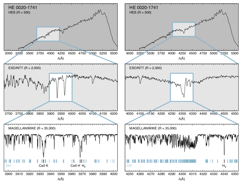
Figure 1.— Spectra of HE 0020$-$1741 (catalog ) with three different resolving powers. Upper panels: Low-resolution ($R\sim 500$) HES objective-prism spectrum. Middle panels: Medium-resolution ($R\sim 2,000$) ESO/NTT spectrum. Lower panels: High-resolution ($R\sim 35,000$) Magellan/MIKE spectrum. The left panels show a zoom-in of the region including the Ca ii H and K lines, and the right panels show a zoom-in of the region surrounding the CH $G$-band. Interesting strong features are identified in the lower panels; the blue lines correspond to individual lines associated with the CH molecule.

II.1. Medium-resolution Spectroscopy

The medium-resolution spectrum of HE 0020$-$1741 (catalog ) was obtained as part of an effort to follow-up CEMP candidates from the HES, as described in Placco et al. (2010, 2011). The observations were carried out in semester 2011B using the EFOSC-2 spectrograph (Buzzoni et al., 1984) mounted on the 3.5m ESO New technology Telescope. The setup made use of Grism7 (600 gr mm^-1), and a 1$\farcs$0 slit with $1\times 1$ on-chip binning, resulting in a wavelength coverage of 3550-5500 Å, resolving power of $R\sim 2,000$, dispersion of 0.96 Å/pixel (with $\sim 2$ pixels per resolution element), and signal-to-noise ratios S/N$\sim 60$ per pixel at 4300 Å. The calibration frames included FeAr exposures (taken following the science observation), quartz-lamp flatfields, and bias frames. All reduction tasks were performed using standard IRAF packages. Table 1 lists basic information on HE 0020$-$1741 (catalog )  and details of the spectroscopic observations at medium and high resolution.

II.2. High-resolution Spectroscopy

A high-resolution spectrum was obtained during the 2015A semester using the Magellan Inamori Kyocera Echelle (MIKE; Bernstein et al., 2003) spectrograph mounted on the 6.5m Magellan-Clay Telescope at Las Campanas Observatory. The observing setup included a $0\farcs 7$ slit with $2\times 2$ on-chip binning, yielding a resolving power of $R\sim 35,000$ (blue spectral range) and $R\sim 28,000$ (red spectral range), with $\sim 3$ pixels per resolution element. The S/N at $4300\,$Å is $\sim 100$ per pixel. MIKE spectra have nearly full optical wavelength coverage ($\sim 3500-8500\,$Å). The data were reduced using the data reduction pipeline developed for MIKE spectra, first described by Kelson (2003).

III. Analysis

III.1. Stellar Parameters

The stellar atmospheric parameters were first obtained from the medium-resolution ESO/NTT spectrum using the n-SSPP (Beers et al., 2014), a modified version of the SEGUE Stellar Parameter Pipeline (SSPP; Lee et al., 2008a, b; Allende Prieto et al., 2008; Lee et al., 2011; Smolinski et al., 2011; Lee et al., 2013). The values for $T_{\mathrm{eff}}$, $\log\,g$, and $[\mathrm{Fe}/\mathrm{H}]$ determined from this analysis were used as first estimates for the high-resolution analysis. Using the high-resolution MIKE spectrum, we determined the stellar parameters spectroscopically, using software developed by Casey (2014). Equivalent-width measurements were obtained by fitting Gaussian profiles to the observed absorption lines. Table 2 lists the lines used in this work, their measured equivalent widths, and the derived abundance from each line. We employed one-dimensional plane-parallel model atmospheres with no overshooting (Castelli & Kurucz, 2004), computed under the assumption of local thermodynamic equilibrium (LTE).

Table 2 Equivalent-Width Measurements

Ion	$\lambda$	$\chi$	$\log\,gf$	$W$	$\log\epsilon$ (X)
	(Å)	(eV)		(mÅ)
C CH	4246.000	$\cdots$	$\cdots$	syn	5.83
C CH	4313.000	$\cdots$	$\cdots$	syn	5.73
N CN	3883.000	$\cdots$	$\cdots$	syn	6.13
Na I	5889.950	0.00	0.108	97.06	2.77
Na I	5895.924	0.00	$-$0.194	83.35	2.79
Mg I	3829.355	2.71	$-$0.208	syn	4.60
Mg I	3832.304	2.71	0.270	syn	4.60
Mg I	3838.292	2.72	0.490	syn	4.60
Mg I	4571.096	0.00	$-$5.688	syn	4.90
Mg I	4702.990	4.33	$-$0.380	syn	4.90

Note. — Table available in its entirety in machine-readable form.

The effective temperature of HE 0020$-$1741 (catalog ) was determined by minimizing trends between the abundances of 77 Fe I lines and their excitation potentials, and applying the temperature corrections suggested by Frebel et al. (2013). The microturbulent velocity was determined by minimizing the trend between the abundances of Fe I lines and their reduced equivalent widths. The surface gravity was determined from the balance of the two ionization stages of iron, Fe I and Fe II. HE 0020$-$1741 (catalog ) also had its stellar atmospheric parameters determined from the moderate-resolution ($R\sim 8,000$) RAVE spectrum by Kordopatis et al. (2013). These values, together with our determinations from the medium- and high-resolution spectra, are listed in Table 3.

There is very good agreement between the temperatures derived from the medium- and high-reslution spectra used in this work; the RAVE value is about $\sim 200$ K warmer. The surface gravities are all within 2$\sigma$, and the ESO/NTT and RAVE values agree with each other exactly. This is expected, since both of these estimates come from isochrone matching, while the high-resolution $\log\,g$ was determined from the balance of Fe I and Fe II lines. For $[\mathrm{Fe}/\mathrm{H}]$, the RAVE value is 0.8 dex higher than the other two results. According to the RAVE Data Release 4 (Kordopatis et al., 2013), the spectrum for HE 0020$-$1741 (catalog ) has a S/N=40, which is below the S/N=50 limit set by Kordopatis et al. (2011) for reliable parameter estimates for halo giants, and their pipeline analysis converged without warnings for this star. Since the difference in temperature cannot alone account for such a large discrepancy in $[\mathrm{Fe}/\mathrm{H}]$, this most likely arises from a combination of the lower S/N and the methods used to calibrate the RAVE metallicity scale for giants, which have a 0.40 dex dispersion in their residuals.

Table 3Derived Stellar Parameters for HE 0020$-$1741 (catalog )

	$T_{\mathrm{eff}}$(K)	$\log\,g$(cgs)	$[\mathrm{Fe}/\mathrm{H}]$	$\xi$(km/s)
RAVE	4974 (101)	0.95 (0.35)	$-$3.20 (0.10)	$\cdots$
ESO/NTT	4792 (150)	0.98 (0.35)	$-$4.06 (0.20)	$\cdots$
Magellan	4765 (100)	1.55 (0.20)	$-$4.05 (0.05)	1.50 (0.20)

Table 4Abundances for Individual Species

Species	$\log\epsilon_{\odot}$ (X)	$\log\epsilon$ (X)	[X/H]	[X/Fe]	$\sigma$	$N$
C (CH)	$+$8.43	$+$5.78	$-$2.65	$+$1.40	0.15	2
C (CH)	$+$8.43	$+$6.12	$-$2.31	$+$1.74	0.15	2
N (CN)	$+$7.83	$+$6.13	$-$1.70	$+$2.35	0.20	1
Na I	$+$6.24	$+$2.78	$-$3.46	$+$0.59	0.05	2
Mg I	$+$7.60	$+$4.58	$-$3.02	$+$1.03	0.10	8
Al I	$+$6.45	$+$2.05	$-$4.40	$-$0.26	0.10	1
Si I	$+$7.51	$+$4.36	$-$3.19	$+$0.90	0.10	1
Ca I	$+$6.34	$+$2.70	$-$3.64	$+$0.40	0.05	4
Sc II	$+$3.15	$-$0.72	$-$3.87	$+$0.18	0.05	3
Ti I	$+$4.95	$+$1.17	$-$3.78	$+$0.27	0.05	4
Ti II	$+$4.95	$+$1.19	$-$3.76	$+$0.28	0.10	11
Cr I	$+$5.64	$+$1.51	$-$4.13	$-$0.09	0.05	5
Mn I	$+$5.43	$+$1.43	$-$4.00	$+$0.05	0.05	4
Fe I	$+$7.50	$+$3.45	$-$4.05	$-$0.00	0.05	77
Fe II	$+$7.50	$+$3.45	$-$4.05	$-$0.00	0.08	3
Co I	$+$4.99	$+$1.29	$-$3.70	$+$0.35	0.05	4
Ni I	$+$6.22	$+$1.94	$-$4.28	$-$0.23	0.05	7
Sr II	$+$2.87	$-$1.91	$-$4.78	$-$0.73	0.07	2
Ba II	$+$2.18	$-$2.97	$-$5.15	$-$1.11	0.05	2
Eu II	$+$0.52	$<-$3.28	$<-$3.80	$<+$0.25	$\cdots$	1
Pb I	$+$1.75	$<-$0.25	$<-$2.00	$<+$2.05	$\cdots$	1

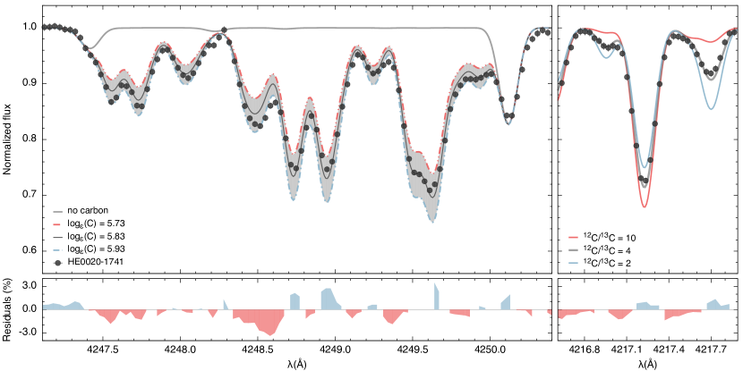
Figure 2.— Left panel: Spectral synthesis of the CH $G$-band for HE 0020$-$1741 (catalog ). The dots represent the observed high-resolution spectrum, the solid line is the best abundance fit, and the dotted and dashed lines are the lower and upper abundances, used to estimate the abundance uncertainty. The gray shaded area encompasses a 0.2 dex difference in $\log\epsilon\,(\mathrm{C})$. The light gray line shows the synthesized spectrum in the absence of carbon. Right panel: Determination of the carbon isotopic ratio, ¹²C/¹³C. The dots represent the observed spectrum, the solid gray line is the best fit, and the colored lines are the lower and upper abundances, used to estimate the uncertainty. The lower panels show the residuals (in %) between the observed data and the best abundance fit.

III.2. Chemical Abundances and Upper Limits

Elemental-abundance ratios, $[\mathrm{X}/\mathrm{Fe}]$, are calculated adopting Solar photospheric abundances from Asplund et al. (2009). The average measurements (or upper limits) for $18$ elements, derived from the Magellan/MIKE spectrum, are listed in Table 4. The $\sigma$ values are the standard error of the mean. Abundances were calculated by both equivalent-width analysis and spectral synthesis. The 2014 version of the MOOG code (Sneden, 1973), which includes a more realistic treatment of scattering (see Sobeck et al., 2011, for further details), is used for the spectral synthesis.

III.2.1 Carbon and Nitrogen

Carbon abundance was derived from CH molecular features at $\lambda$4246 ($\log\epsilon\,(\mathrm{C})$=5.83) and $\lambda$4313 ($\log\epsilon\,(\mathrm{C})$=5.73), with an average value of $\log\epsilon\,(\mathrm{C})$=5.78 ($[\mathrm{C}/\mathrm{Fe}]$$=+1.40$). The left panels of Figure 2 show the spectral synthesis of the CH $G$-band for HE 0020$-$1741 (catalog ). The dots represent the observed spectra, the solid line is the best abundance fit, and the dotted and dashed lines are the lower and upper abundances, used to estimate the uncertainty. The gray line shows the synthesized spectrum in the absence of carbon. The lower panel shows the residuals (in %) between the observed data and the best abundance fit, which are all below 3% for the synthesized region. Since HE 0020$-$1741 (catalog ) is on the upper red-giant branch, the observed carbon abundance does not reflect the chemical composition of its natal gas cloud. By using the procedure described in Placco et al. (2014a), which interpolates the observed $\log\,g$, $[\mathrm{Fe}/\mathrm{H}]$, and $[\mathrm{C}/\mathrm{Fe}]$ of HE 0020$-$1741 (catalog ) with a grid of theoretical stellar evolution models for low-mass stars, we determine the carbon depletion due to CN processing for HE 0020$-$1741 (catalog ) to be 0.34 dex.

The ¹²C/¹³C isotopic ratio is a sensitive indicator of the extent of mixing processes in stars on the red-giant branch. Using a fixed elemental carbon abundance ($\log\epsilon\,(\mathrm{C})$=5.78) for the CH features around $\lambda$4217 Å, we derived ¹²C/¹³C = 4, which suggests that substantial processing of ¹²C into ¹³C has taken place in the star. We note that this ratio also indicates that considerable processing of carbon into nitrogen has occured in HE 0020$-$1741 (catalog ). The right panels of Figure 2 show the determination of the ¹²C/¹³C isotopic ratio. The dots represent the observed spectrum, the solid gray line is the best fit, with the two other values taken to be lower and upper limits. The lower panel shows that the residuals between the observed data and ¹²C/¹³C = 4 are all below 2%.

The nitrogen abundance was determined from spectral synthesis of the CN band at $\lambda$3883 Å. The NH band at $\lambda$3360 Å did not have sufficiently high S/N to allow for a proper spectral synthesis. For the CN band, we used a fixed carbon abundance of $\log\epsilon\,(\mathrm{C})$=5.78 (average of carbon abundances determined from the CH band), and derived a value of $\log\epsilon\,(\mathrm{N})$=6.13, with an uncertainty of $\pm 0.2$ dex.

III.2.2 From Na to Ni

Abundances of Na, Sc, Ti, Cr, Co, and Ni were determined by equivalent-width analysis only. For Ti, where transitions from two different ionization stages were measured, the abundances agree within 0.02 dex. Spectral synthesis was used to determine abundances for Mg, Al, Si, Ca, and Mn (accounting for hyperfine splitting from the linelists from Den Hartog et al., 2011).

III.2.3 Neutron-capture Elements

The chemical abundances for Sr and Ba, as well as upper limits for Eu and Pb, were determined via spectral synthesis. We used the compilation of linelists by Frebel et al. (2014), based on lines from Aoki et al. (2002), Barklem et al. (2005), Lawler et al. (2009), and the VALD database (Kupka et al., 1999). The neutron-capture absorption lines in the blue spectral region, particularly close to strong CH or CN features, need to be carefully synthesized, since these are intrinsically weak in CEMP-no stars. Because of that, we included the observed carbon and nitrogen abundances for all the syntheses, as well as the ¹²C/¹³C isotope ratio.

The Sr abundance was determined from the $\lambda$4077 ($\log\epsilon\,(\mathrm{Sr})$ = $-$1.93) and $\lambda$4215 ($\log\epsilon\,(\mathrm{Sr})$ = $-$1.88) lines, with an average value of $[\mathrm{Sr}/\mathrm{Fe}]$ = $-$0.73. For Ba, both $\lambda$4554 and $\lambda$4934 features were successfully synthesized with $\log\epsilon\,(\mathrm{Ba})$ = $-$2.97 ($[\mathrm{Ba}/\mathrm{Fe}]$ = $-$1.11). Both Sr and Ba abundances are within typical ranges for CEMP-no stars (Placco et al., 2014a).

Upper limits were determined for Eu ($\lambda$4129) and Pb ($\lambda$4057). The Pb upper limit ($[\mathrm{Pb}/\mathrm{Fe}]$$<+$2.05) is similar to the one for the CEMP-no BD+44^∘493 (catalog ) (Placco et al., 2014c), and it adds further evidence that the origin of the neutron-capture abundances in HE 0020$-$1741 (catalog ) is unlikely to be from an unseen evolved companion. The $[\mathrm{Pb}/\mathrm{Fe}]$ should be higher by at least a factor of ten to agree with theoretical predictions for the $s$-process (Bisterzo et al., 2010). Furthermore, the radial-velocity monitoring of HE 0020$-$1741 (catalog ) reported by Hansen et al. (2016) revealed no significant variation ($\sigma=0.212$ km s^-1) over a temporal window of 1066 days.

Table 5Example Systematic Abundance Uncertainties for HE 0020$-$1741 (catalog )

Elem	$\Delta$$T_{\mathrm{eff}}$	$\Delta$$\log\,g$	$\Delta\xi$	$\sigma/\sqrt{n}$	$\sigma_{\rm tot}$
	$+$150 K	$+$0.3 dex	$+$0.3 km/s
Na I	0.14	$-$0.04	$-$0.11	0.07	0.20
Mg I	0.13	$-$0.12	$-$0.07	0.04	0.19
Al I	0.11	$-$0.07	$-$0.11	0.10	0.20
Si I	0.14	$-$0.02	$-$0.01	0.10	0.17
Ca I	0.10	$-$0.02	$-$0.01	0.05	0.11
Sc II	0.09	0.07	$-$0.04	0.06	0.13
Ti I	0.17	$-$0.03	$-$0.01	0.05	0.18
Ti II	0.06	0.06	$-$0.08	0.03	0.12
Cr I	0.17	$-$0.04	$-$0.06	0.04	0.19
Mn I	0.19	$-$0.05	$-$0.07	0.07	0.22
Fe I	0.16	$-$0.05	$-$0.09	0.01	0.19
Fe II	0.01	0.09	$-$0.02	0.08	0.12
Co I	0.18	$-$0.03	$-$0.02	0.05	0.19
Ni I	0.17	$-$0.07	$-$0.09	0.04	0.21
Sr II	0.09	0.06	$-$0.10	0.07	0.16
Ba II	0.12	0.08	$-$0.01	0.07	0.16

III.3. Uncertainties

Uncertainties in the elemental-abundance determinations, as well as the systematic uncertainties due to changes in the atmospheric parameters, were treated in the same way as described in Placco et al. (2013, 2015b). Table 5 shows how variations within the quoted uncertainties in each atmospheric parameter affect the derived chemical abundances. Also listed is the total uncertainty for each element, which is calculated from the quadratic sum of the individual error estimates. Even though $T_{\mathrm{eff}}$, $\log\,g$, and $\xi$ are correlated, we assume complete knowledge of two of them to assess how changes in the third parameter would affect the abundance calculation. For example, a change in $+$150 K in $T_{\mathrm{eff}}$ for HE 0020$-$1741 (catalog ) requires a change of about 0.1 dex in $\log\,g$ to maintain the balance between Fe I and Fe II. However, this change in $\log\,g$ translates to a 0.01 dex change in abundance, which is 16 times smaller than the change due to $T_{\mathrm{eff}}$. Then, for simplicity, we assume that the variables are independent, and use the quadratic sum. For this calculation, we used spectral features with abundances determined by equivalent-width analysis only. The variations for the parameters are $+$150 K for $T_{\mathrm{eff}}$, $+$0.3 dex for $\log\,g$, and $+$0.3 km s^-1 for $\xi$.

IV. Discussion

IV.1. Model Predictions for UMP Progenitors

In this section, we assess the main properties of the possible stellar progenitors of selected UMP stars from the literature, by comparing their abundance patterns with theoretical model predictions for Pop III stars. We employ the non-rotating massive-star models from Heger & Woosley (2010), for which the free parameters are the mass ($10\,\mathrm{M}_{\odot}-100\,\mathrm{M}_{\odot}$), explosion energies ($0.3-10\times 10^{51}\,\mathrm{erg}$), and the amount of mixing in the SNe ejecta. The grid used in the work has 16,800 models, and the $\chi^{2}$ matching algorithm is described in Heger & Woosley (2010). An online tool with the model database can be accessed at starfit. For the present application, we adopt a similar procedure as the one described in Placco et al. (2015a) and Roederer et al. (2016), as described below.

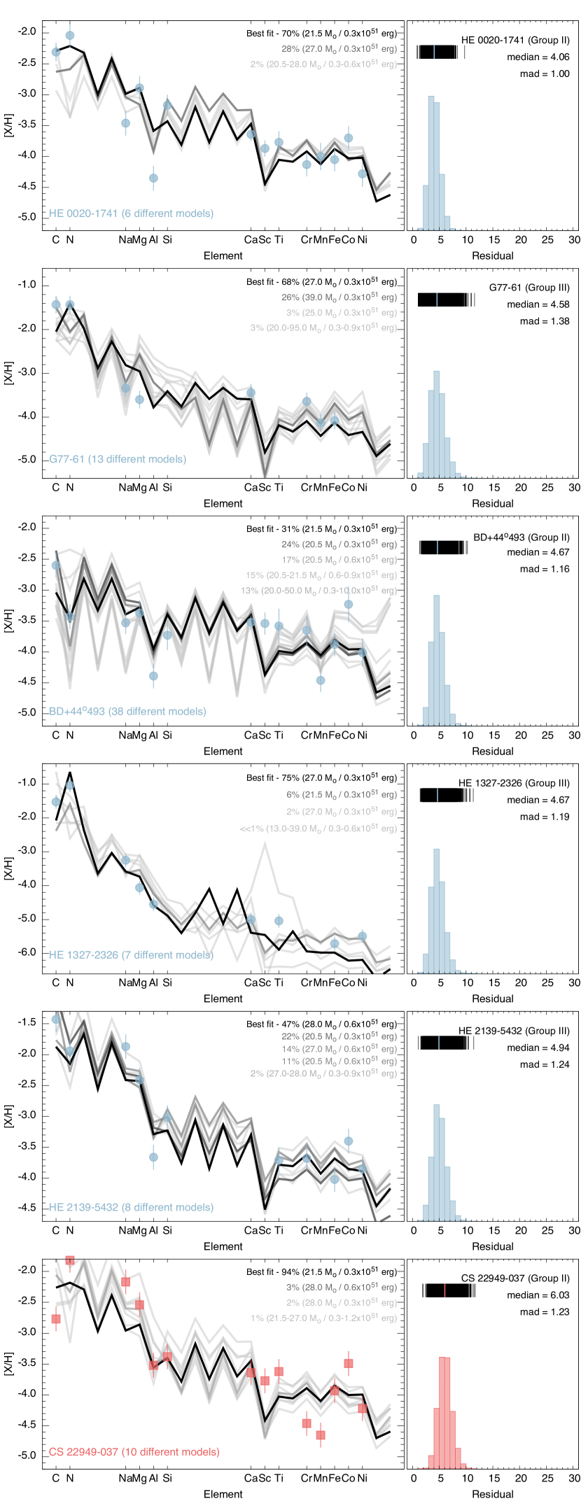
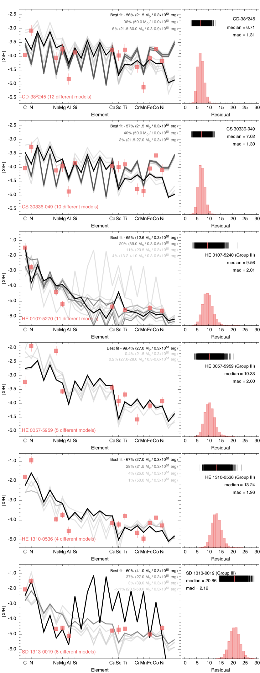
Figure 3.— Best model fits for HE 0020$-$1741 (catalog ) and the 11 other UMP stars from the literature, ordered by increasing median residuals. For each star, the left panel shows the simulated abundance patterns and models, where the masses and explosion energies are provided in the legend at the upper right of each panel, color-coded by their fractional occurence. The right panel shows the distribution of the residuals for the 10,000 simulations for each star. The colored bar overlaying the upper density distributions in the right panels marks the median value, which is shown in the legend of each panel at the top right, along with the $mad$ (median absolute deviation).

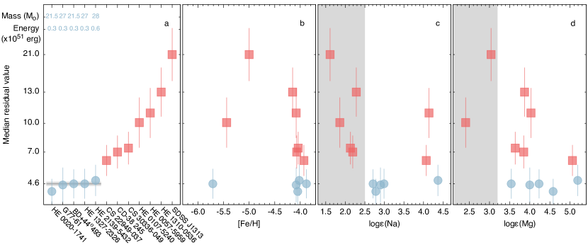
Figure 4.— Median residuals for HE 0020$-$1741 (catalog ) and 11 other UMP stars from the literature, color-coded by the division proposed in Figure 3. The stars are ordered by increasing median values (Panel $a$). The solid horizontal line shows the median for the five stars with low residuals, and the gray shaded areas encompass $\pm 1\times mad$ and $\pm 2\times mad$. The numbers on the top are the progenitor masses (in M_⊙) and explosion energy ($\times 10^{51}\,\mathrm{erg}$) from the best model fit for each star. Panels $b$, $c$, and $d$ show the residuals as a function of $[\mathrm{Fe}/\mathrm{H}]$, $\log\epsilon\,(\mathrm{Na})$, and $\log\epsilon\,(\mathrm{Mg})$, respectively.

We collected UMP stars from the literature for which at least carbon, nitrogen, sodium, magnesium, calcium, and iron were measured. With $[\mathrm{Fe}/\mathrm{H}]$$<-4.0$, only 11 stars have abundances for these elements determined from high-resolution spectroscopy (including HE 0020$-$1741 (catalog )). We also added BD+44^∘493 (catalog ) to the sample, since its metallicity is $[\mathrm{Fe}/\mathrm{H}]$ = $-$3.8, and it has a number of abundances measured with small uncertainties. Table IV.1 lists the abundances and references for the literature sample. The stars are divided according to the CEMP-no Groups II and III from Yoon et al. (2016); two of our sample stars are classified as carbon-normal stars. The carbon abundances were corrected for the C depleted by CN processing, following the procedures described in Placco et al. (2014b), and briefly summarized in Section III.2.1. In addition, we calculated the inverse corrections for the nitrogen abundances, by imposing that the [(C$+$N)/Fe] ratio remains constant throughout the evolution of the star on the giant branch. The model grid we employed is the same as that in Placco et al. (2014b). Even though there may also be ON processing that occurs in the star, the effect is expected to be negligible compared to the CN processing (see bottom panel of Figure 2 in Placco et al., 2014b).

For the model matching, we have used the following abundances (where available): C, N, Na, Mg, Al, Si, Ca, Sc, Ti, V, Cr, Mn, Fe, Co, and Ni. For consistency, no upper limits were used. For each star, we assembled $10^{4}$ unique abundance patterns, based on the observed values from the literature. For each element, we generated $10^{4}$ random numbers from a normal distribution, with the measured abundances as the central value, and the uncertainties as the dispersion. Then, we randomly selected individual abundances from each distribution, and generated new abundance patterns. For each of these, we found the progenitor mass, explosion energy, and the mean squared residuals from the starfit code.

Figure 3 shows the results of this exercise for the 12 stars in Table IV.1. For each star, the left panel shows the best model fits for the $10^{4}$ abundance patterns. The masses and explosion energies of the models are given in the legend at the upper right in each panel, color-coded by their fractional occurence. The right-hand panel for each star shows the distribution of the mean squared residuals for the simulations. The colored bars overlaying the upper density distributions on the right panels mark the median residual value, and its value is shown in the legend of these panel at the top right, along with the $mad$ (median absolute deviation), a robust estimator of the dispersion. The stars are ordered by increasing median values.

As an example, consider the top left panel of Figure 3, for the star HE 0020$-$1741 (catalog ). We first ran the starfit code to find the best model fit for each of the $10^{4}$ abundance patterns generated from the observed abundances (blue filled circles). In about 70% (7,041) of the resampled abundance patterns, the best fit was the model with $21.5\,\mathrm{M}_{\odot}$ and $0.3\times 10^{51}\,\mathrm{erg}$ (black solid line). In 2,849 (28%) of the patterns, the model with $27.0\,\mathrm{M}_{\odot}$ and $0.3\times 10^{51}\,\mathrm{erg}$ gave the best fit (dark gray solid line), and for the remaining 110 abundance patterns (light gray solid lines), the best-fit models had masses between $20.5-28.0\,\mathrm{M}_{\odot}$ and explosion energies between $0.3-0.6\times 10^{51}\,\mathrm{erg}$. In total, 6 unique models (out of the 16,800 models on the grid) were able to account for the best fits for the $10^{4}$ resampled abundance patterns. For each best fit, the starfit code calculates the mean squared residual, and the distribution of these values is given on the panel to the right side of the abundance patterns. Above the distribution is the density plot (black stripes), with the median value (blue stripe) shown on the upper right part of the panel, together with the $mad$.

For the first five stars in the left-hand column of panels shown in Figure 3, the mass and explosion energy of the progenitor are within $20.5-28.0\,\mathrm{M}_{\odot}$ and $0.3-0.6\times 10^{51}\,\mathrm{erg}$. These values are consistent with predictions from Nomoto et al. (2006) for the faint supernova progenitor scenario. Considering the two most-frequent models for each star, the C-N abundances are well-reproduced in most cases, within $2\sigma$ of the theoretical values. The Na-Si abundances agree within $2\sigma$ with the best model fits (except for Al in HE 0020$-$1741 (catalog ) and Mg in G77$-$61 (catalog )). The Ca and Ti abundances also agree within $2\sigma$, except for Ti in HE 1327$-$2326 (catalog ). The large over-abundances of Sc for HE 0020$-$1741 (catalog ) and BD$+$44^∘493 (catalog ) are expected, since Sc may have contributions from other nucleosynthesis processes (see Heger & Woosley, 2010, for further details). Among the Cr-Fe abundances, there is also overall good agreement, with Fe values agreeing within $1\sigma$ with the best model fits. The enhanced cobalt abundances for HE 0020$-$1741 (catalog ), BD$+$44^∘493 (catalog ), and HE 2139$-$5432 (catalog ) cannot be accounted for by the models, but we note that $\log\epsilon\,(\mathrm{Co})$ is often under-predicted by theoretical models (e.g., Tominaga et al., 2014; Roederer et al., 2016).

For stars in the right-hand panels of Figure 3 (red filled squares), the progenitor masses range from $12.6\,\mathrm{M}_{\odot}$ for HE 0107$-$5240 (catalog ) to $41.0\,\mathrm{M}_{\odot}$ for SDSS J1313$-$0019 (catalog ), all with explosions energies of $0.3\times 10^{51}\,\mathrm{erg}$. For these stars, as reflected by their residual distributions, there is a clear mismatch between the model predictions and the observed abundances. The stars CS 22949$-$037 (catalog ), CD$-$38^∘245 (catalog ), and CS 30336$-$049 (catalog ) all have best fits with a $21.5\,\mathrm{M}_{\odot}$ and $0.3\times 10^{51}\,\mathrm{erg}$ model. This is likely a numerical artifact, since the C and N abundances for these three stars are in complete disagreement with the models. For HE 0057$-$5959 (catalog ), only the Ca abundance matches the best model yields, and most values are at least 0.5 dex away from the theoretical values. For HE 1310$-$0536 (catalog ), the only observed abundance within $1\sigma$ of the model is Fe. In this case, it is clear that no models can reproduce the large difference between the C-N and Na-Al abundances. For HE 0107$-$5240 (catalog ) and SDSS J1313$-$0019 (catalog ), the models are not able to simultaneously predict the C-N abundances and the Na-Mg or Ca-Ti abundances.

Based on these results, we infer that the first five stars shown in the left-hand column of panels of Figure 3 have abundance patterns that are consistent with the progenitor stellar population described by the models of Heger & Woosley (2010). For the remaining seven stars, the poor agreement between observations and models suggests the presence of at least one additional class of stellar progenitors for UMP stars.

Figure 4 shows the behavior of the median residual values for HE 0020$-$1741 (catalog ) and the data for other UMP stars from the literature, where the stars are ordered by increasing median values (Panel $a$), and as a function of $[\mathrm{Fe}/\mathrm{H}]$ (Panel $b$), $\log\epsilon\,(\mathrm{Na})$ (Panel $c$), and $\log\epsilon\,(\mathrm{Mg})$ (Panel $d$). In Panel $a$, the gray shaded areas encompass $\pm 1\times mad$ and $\pm 2\times mad$ for the five stars (blue filled circles) in the left-hand column of Figure 3. The numbers shown in the legend are the progenitor masses (in M_⊙) and the explosion energy ($\times 10^{51}\,\mathrm{erg}$) from the best model fit for each star. The gray regions highlighted on Panels $c$ and $d$ are explained below.

Distinctions between the stars with low (blue symbols) and high (red symbols) residuals become more evident when inspecting the median residuals in Figure 4. Even though this separation does not appear to be correlated with $[\mathrm{Fe}/\mathrm{H}]$ (Panel $b$), observations of additional stars are needed to cover the gap between $-5.0\leq$ $[\mathrm{Fe}/\mathrm{H}]$ $\leq-4.0$, in order to uncover any possible trend. Nevertheless, HE 1327$-$2326 (catalog ) ($[\mathrm{Fe}/\mathrm{H}]$ = $-5.71$) has a median residual value consistent with that of other stars at $[\mathrm{Fe}/\mathrm{H}]$ $\sim-4.0$, and it does not agree with the values for HE 0107$-$5240 (catalog ) ($[\mathrm{Fe}/\mathrm{H}]$ = $-5.44$) and SDSS J1313$-$0019 (catalog ) ($[\mathrm{Fe}/\mathrm{H}]$ = $-5.00$). From inspection of Panel $c$, it can be seen that the low-residual stars exhibit $\log\epsilon\,(\mathrm{Na})$ $\gtrsim 2.5$, and are mostly concentrated at $\log\epsilon\,(\mathrm{Na})$ $\sim 2.8$. The only exception is HE 2139$-$5432 (catalog ), with $\log\epsilon\,(\mathrm{Na})$ $=4.37$. The trend for Na can be an indication that another stellar progenitor, producing (but not limited to) $\log\epsilon\,(\mathrm{Na})$ $\lesssim 2.5$ (gray shaded area on Panel $c$), is needed to account for the diferences in the observed abundances. In Panel $d$, even though the low-residual stars exhibit $\log\epsilon\,(\mathrm{Mg})$ $\gtrsim 3.5$, there is no obvious separation between these and the high-residual stars. The two high-residual stars with low $\log\epsilon\,(\mathrm{Na})$ in Panel $c$ also have low $\log\epsilon\,(\mathrm{Mg})$. However, this correlation does not hold for the other stars in the same group.

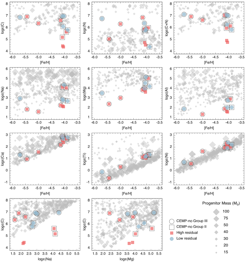
Figure 5.— Comparison between the chemical abundances of the literature sample of UMP stars (colored symbols) and the predicted yields from the supernovae models used in this work (gray symbols). The progenitor mass is proportional to the size of the symbol. The open symbols relate to the CEMP-no classifications proposed by Yoon et al. (2016).

Table 6Literature data ($\log\epsilon\,(\mathrm{X})$ abundances)

Star name	C	N	Na	Mg	Al	Si	Ca	Sc	Ti	Cr	Mn	Fe	Co	Ni	Ref.	Note
CEMP-no Group II
BD$+$44∘493	5.83	4.40	2.71	4.23	2.06	3.78	2.82	$-$0.39	$-$1.37	1.99	0.97	3.62	1.76	2.21	1	$\cdots$
CS 22949$-$037	5.66	6.01	4.07	5.06	2.93	4.13	2.70	$-$0.62	$-$1.33	1.18	0.78	3.57	1.50	2.00	2	a
HE 0020$-$1741	6.12	5.79	2.78	4.58	2.05	4.36	2.70	$-$0.72	$-$1.18	1.51	1.43	3.45	1.29	1.94	3	b
HE 0057$-$5959	5.21	5.90	4.14	4.03	$\cdots$	$\cdots$	2.91	$-$0.76	$-$1.27	1.06	$\cdots$	3.42	$\cdots$	2.30	4	$\cdots$
CEMP-no Group III
G77$-$61	7.00	6.40	2.90	4.00	$\cdots$	$\cdots$	2.90	$\cdots$	$\cdots$	2.00	1.30	3.42	$\cdots$	$\cdots$	5	$\cdots$
HE 0107$-$5240	6.96	5.57	1.86	2.41	$\cdots$	$\cdots$	0.99	$\cdots$	$-$0.62	$\cdots$	$\cdots$	2.06	$\cdots$	0.60	6	c
HE 1310$-$0536	6.64	6.88	2.28	3.87	1.91	$\cdots$	2.19	$-$1.07	$-$1.15	1.00	0.49	3.35	1.12	1.95	7	d
HE 1327$-$2326	6.90	6.79	2.99	3.54	1.90	$\cdots$	1.34	$\cdots$	$-$0.09	$\cdots$	$\cdots$	1.79	$\cdots$	0.73	8	$\cdots$
HE 2139$-$5432	7.00	5.89	4.37	5.19	2.79	4.49	$\cdots$	$\cdots$	$-$1.24	1.96	$\cdots$	3.48	1.59	2.37	9	$\cdots$
SDSS J1313$-$0019	6.39	6.34	1.61	3.04	1.34	$\cdots$	1.59	$-$1.54	$-$0.33	$\cdots$	$\cdots$	2.50	$\cdots$	1.65	10	$\cdots$
Carbon-Normal Stars
CD$-$38∘245	4.48	4.76	2.19	3.85	1.63	3.65	2.56	$-$0.82	$-$1.19	1.25	0.31	3.43	1.25	2.05	11	e
CS 30336$-$049	4.40	4.56	2.13	3.64	1.58	3.66	2.39	$-$0.83	$-$1.06	0.86	0.57	3.46	1.42	2.13	12	f

References. —

(1): Ito et al. (2013);

(2): Cohen et al. (2013);

(3): This work;

(4): Yong et al. (2013a);

(5): Plez & Cohen (2005);

(6): Christlieb et al. (2004);

(7): Hansen et al. (2015);

(8): Frebel et al. (2008);

(9): Yong et al. (2013a);

(10): Frebel et al. (2015).

(11): François et al. (2003);

(12): Lai et al. (2008);

Note. —

(a): $\Delta$$\log\epsilon\,(\mathrm{C})$ = $+0.15$, $\Delta$$\log\epsilon\,(\mathrm{N})$ = $-0.09$;

(b): $\Delta$$\log\epsilon\,(\mathrm{C})$ = $+0.34$, $\Delta$$\log\epsilon\,(\mathrm{N})$ = $-0.34$;

(c): Average of C and N values;

(d): $\Delta$$\log\epsilon\,(\mathrm{C})$ = $+0.07$, $\Delta$$\log\epsilon\,(\mathrm{N})$ = $0.00$;

(e): $\log\epsilon\,(\mathrm{C})$ from McWilliam et al. (1995), $\log\epsilon\,(\mathrm{N})$ from Spite et al. (2006), $\Delta$$\log\epsilon\,(\mathrm{C})$ = $+0.07$, $\Delta$$\log\epsilon\,(\mathrm{N})$ = $-0.04$;

(f): $\Delta$$\log\epsilon\,(\mathrm{C})$ = $+0.29$, $\Delta$$\log\epsilon\,(\mathrm{N})$ = $-0.15$;

IV.2. Abundance Comparison between UMP Stars and Yields from Massive Metal-free Stars

To further investigate the differences among the twelve UMP stars, we compared the individual abundances as a function of $[\mathrm{Fe}/\mathrm{H}]$, $\log\epsilon\,(\mathrm{Na})$, and $\log\epsilon\,(\mathrm{Mg})$ with the yields from the 16,800 models used for the matching procedure. Figure 5 shows the result of this exercise. The colored symbols are the observed abundances from the literature sample (including HE 0020$-$1741 (catalog )), and the gray symbols are yields from the supernova models. The open symbols show the CEMP-no groups proposed in Paper I. For the theoretical values, the progenitor mass is proportional to the size of the symbol. Models with abundance values outside the ranges shown in Figure 5 were suppressed for simplicity.

Overall, the twelve stars have abundances consistent with the models for the elements Ca, Ti, and Ni. This also holds true for other elements not shown in Figure 5, such as Cr, Mn, and Co. Abundances for the five low-residual stars (blue filled circles) present, in general, good agreement with the values predicted by models with M $<30\,\mathrm{M}_{\odot}$. Some exceptions include: $\log\epsilon\,(\mathrm{N})$ for G77$-$61 (catalog ) and HE 1327$-$2326 (catalog ) (however, $\log\epsilon\,(\mathrm{C+N})$ agrees well in both cases); $\log\epsilon\,(\mathrm{Al})$ for HE 0020$-$1741 (catalog ) and BD$+$44^∘493 (catalog ) is about 0.5 dex lower than the model values. Even though the Al abundance was determined from spectral synthesis, that region ($\lambda$3961 Å) presents strong CH and CN absorption features, which could compromise the determination. For the seven stars with higher median residual values, there are clear mismatches between the observations and the theoretical predictions. For CD$-$38^∘245 (catalog ) and CS 30336$-$049 (catalog ), carbon and nitrogen are at least 1 dex lower than the model values, and Na, Mg, and Al are also below the model ranges. Even though CS 22949$-$037 (catalog ) exhibits better agreement for C and N, the two bottom panels show that four stars are below the model expectations for $\log\epsilon\,(\mathrm{C})$ vs. $\log\epsilon\,(\mathrm{Na})$ and $\log\epsilon\,(\mathrm{C})$ vs. $\log\epsilon\,(\mathrm{Mg})$. There is also no agreement for Na, Mg, and Al (HE 0107$-$5240 (catalog ) and SDSS J1313$-$0019 (catalog )) as a function of metallicity.

Inspection of the two bottom panels of Figure 5 reveals that C, Na, and Mg abundances may suggest some deficiencies in the current models, which could exclude these as possible progenitors for four of the seven high-residual stars. In both cases, the carbon abundances are over-predicted by the models when compared to the observations. This suggests that the current models do not adequately capture the progenitors of the full set of UMP stars. The combination of carbon, sodium, and magnesium was used in Paper I as part of the justification for the division of the CEMP-no stars in Groups II and III. When comparing the low- and high-residual stars with their CEMP-no group classifications, it can be seen that half of the Group II stars (HE 0107$-$5240 (catalog ) and SDSS J1313$-$0019 (catalog )) are outside the model ranges for $\log\epsilon\,(\mathrm{C})$ vs. $\log\epsilon\,(\mathrm{Na})$ and $\log\epsilon\,(\mathrm{C})$ vs. $\log\epsilon\,(\mathrm{Mg})$. The two other Group II stars (HE 0020$-$1741 (catalog ) and BD$+$44^∘493 (catalog )) have low median residuals, and are close to the limits explored by the models. Another interesting case is HE 1327$-$2326 (catalog ) (Group III), which is the most metal-poor star in this sample; it presents a low median residual, unlike the other stars with $[\mathrm{Fe}/\mathrm{H}]$$<-5.0$. Its chemical abundances are in regions where the model grid is sparse, specially for C, N, Na, and Mg. Regardless, the models used in this work cannot account for the abundance patterns of HE 0107$-$5240 (catalog ) and SDSS J1313$-$0019 (catalog ), which are also Group III stars based on Paper I. This could be further evidence that at least one additional, different progenitor population operates at the lowest metallicities, such as the spinstars described by Meynet et al. (2006).

For completeness, we also tested the robustness of our fitting results with respect to the recent study of Ezzeddine et al. (2016, in preparation). This study suggests the presence of large positive corrections to the Fe abundances of the 18 most iron-poor stars, following line formation computations in a non local thermodynamic equilibrium (NLTE). While it would be inconsistent to mix LTE and NLTE abundances in a given stellar pattern, we tested how trial corrections for $\log\epsilon\,(\mathrm{Fe})$ of 0.75 dex to HE 1327$-$2326 (catalog ), 0.70 dex to HE 0107$-$5240 (catalog ), and 0.3 dex to HE 0020$-$1741 (catalog ) would affect our conclusions. As a result, no significant changes in the progenitor mass, explosion energy, and mean squared residuals were found. To properly interpret these new NLTE Fe abundances, we thus have to await the full NLTE abundance patterns and compare those with the supernova yields, once available.

V. Conclusions

We have presented the first high-resolution spectroscopic study of the ultra metal-poor, CEMP-no star HE 0020$-$1741 (catalog ). This star adds to the small number of stars with $[\mathrm{Fe}/\mathrm{H}]$ $<-4.0$ identified to date, and presents the same behavior as most (more than 80%) of UMP stars: $[\mathrm{C}/\mathrm{Fe}]$$>+1.0$ and $[\mathrm{Ba}/\mathrm{Fe}]$$<0.0$. We have attempted to characterize the progenitor stellar population of UMP stars by comparing the yields from a grid of metal-free, massive-star models with the observed elemental abundances for HE 0020$-$1741 (catalog ) and 11 other UMP stars from the literature for which at least abundances of C, N, Na, Mg, Al, and Fe have been reported.

Based on our residual analysis, we find that 42% (5 of 12) of the sample stars have elemental-abundance patterns that are well-reproduced by the SNe models of Heger & Woosley (2010). We conclude that this class of SNe explosions and their associated nucleosynthesis cannot alone account for the observed abundance patterns of the entire set of UMP stars we have considered. In particular, Pop III, massive metal-free star models cannot reproduce abundance patterns of stars with $\log\epsilon\,(\mathrm{C})$ $\leq 5.0$, $\log\epsilon\,(\mathrm{Na})$  $\lesssim 2.5$, and $\log\epsilon\,(\mathrm{Mg})$  $\lesssim 3.2$. Carbon and sodium could potentially be used as tracers of the stellar progenitor, in addition to the metallicity. This could be evidence of different progenitor signatures, such as fast-rotating massive Pop III stars from Meynet et al. (2006), or the faint SNe from Nomoto et al. (2006). If we assume that the models used in this work are a viable candidate for the stellar progenitors of UMP stars, there must exist at least one additional class of progenitor operating at $[\mathrm{Fe}/\mathrm{H}]$$<-4.0$, or a single process, yet to be identified, that could account for the abundances of all UMP stars. We should also acknowledge the possibility that more than one progenitor could contribute to the observed abundance patterns of the high-residual stars presented in this work.

Recent evidence presented by Yoon et al. (2016) suggests that the carbon abundance may be key to differentiate between different stellar progenitors of UMP stars. The classifications based on absolute carbon abundances, $A$(C), are further confirmed when looking at the sodium and magnesium abundances. The analysis presented in this paper supports this hypothesis, and suggests that the progenitor population(s) for UMP stars may be even more rich and complex than previously thought. We emphasize that abundances for additional UMP stars, in particular those in the metallicity regime $-5.0<$ [Fe/H] $<-4.0$, are needed to better constrain the nature of the possible stellar progenitors. Nitrogen abundances are an important constraint to the theoretical models, and currently more than half of the observed UMP stars have only limits for this element reported.

Table 7 Equivalent-Width Measurements

Ion	$\lambda$	$\chi$	$\log\,gf$	$W$	$\log\epsilon$ (X)
	(Å)	(eV)		(mÅ)
C CH	4246.000	$\cdots$	$\cdots$	syn	5.83
C CH	4313.000	$\cdots$	$\cdots$	syn	5.73
N CN	3883.000	$\cdots$	$\cdots$	syn	6.13
Na I	5889.950	0.00	0.108	97.06	2.77
Na I	5895.924	0.00	$-$0.194	83.35	2.79
Mg I	3829.355	2.71	$-$0.208	syn	4.60
Mg I	3832.304	2.71	0.270	syn	4.60
Mg I	3838.292	2.72	0.490	syn	4.60
Mg I	4571.096	0.00	$-$5.688	syn	4.90
Mg I	4702.990	4.33	$-$0.380	syn	4.90
Mg I	5172.684	2.71	$-$0.450	syn	4.25
Mg I	5183.604	2.72	$-$0.239	syn	4.25
Mg I	5528.405	4.34	$-$0.498	syn	4.85
Al I	3961.520	0.01	$-$0.340	syn	2.05
Si I	4102.936	1.91	$-$3.140	syn	4.36
Ca I	4454.780	1.90	0.260	syn	2.64
Ca I	5588.760	2.52	0.210	4.87	2.71
Ca I	6122.220	1.89	$-$0.315	8.78	2.75
Ca I	6162.170	1.90	$-$0.089	11.92	2.68
Sc II	4246.820	0.32	0.240	57.45	$-$0.75
Sc II	4400.389	0.61	$-$0.540	13.70	$-$0.69
Sc II	4415.544	0.59	$-$0.670	10.63	$-$0.72
Ti I	3989.760	0.02	$-$0.062	10.92	1.14
Ti I	4533.249	0.85	0.532	6.36	1.19
Ti I	4981.730	0.84	0.560	7.55	1.17
Ti I	4991.070	0.84	0.436	6.31	1.20
Ti II	3759.291	0.61	0.280	85.34	1.10
Ti II	3761.320	0.57	0.180	84.26	1.12
Ti II	4012.396	0.57	$-$1.750	26.82	1.30
Ti II	4417.714	1.17	$-$1.190	23.80	1.31
Ti II	4443.801	1.08	$-$0.720	39.21	1.07
Ti II	4450.482	1.08	$-$1.520	17.08	1.34
Ti II	4468.517	1.13	$-$0.600	42.03	1.07
Ti II	4501.270	1.12	$-$0.770	37.73	1.13
Ti II	4533.960	1.24	$-$0.530	42.09	1.12
Ti II	4563.770	1.22	$-$0.960	29.43	1.25
Ti II	4571.971	1.57	$-$0.320	38.54	1.23
Cr I	4254.332	0.00	$-$0.114	57.03	1.50
Cr I	4274.800	0.00	$-$0.220	52.38	1.48
Cr I	4289.720	0.00	$-$0.370	49.12	1.56
Cr I	5206.040	0.94	0.020	19.37	1.48
Cr I	5208.419	0.94	0.160	26.73	1.52
Mn I	4041.380	2.11	$-$0.350	syn	1.43
Mn I	4754.021	2.28	$-$0.647	syn	1.43
Mn I	4783.424	2.30	$-$0.736	syn	1.43
Mn I	4823.514	2.32	$-$0.466	syn	1.43
Fe I	3727.619	0.96	$-$0.609	70.55	3.28
Fe I	3743.362	0.99	$-$0.790	65.97	3.32
Fe I	3753.611	2.18	$-$0.890	16.00	3.41
Fe I	3758.233	0.96	$-$0.005	97.02	3.50
Fe I	3763.789	0.99	$-$0.221	80.31	3.23
Fe I	3765.539	3.24	0.482	13.97	3.20
Fe I	3767.192	1.01	$-$0.390	78.19	3.35
Fe I	3786.677	1.01	$-$2.185	15.44	3.30
Fe I	3820.425	0.86	0.157	105.31	3.33
Fe I	3824.444	0.00	$-$1.360	82.76	3.28
Fe I	3886.282	0.05	$-$1.080	96.13	3.48
Fe I	3887.048	0.91	$-$1.140	57.68	3.22
Fe I	3899.707	0.09	$-$1.515	80.32	3.39
Fe I	3902.946	1.56	$-$0.442	57.99	3.30
Fe I	3917.181	0.99	$-$2.155	25.67	3.51
Fe I	3920.258	0.12	$-$1.734	72.13	3.33
Fe I	3922.912	0.05	$-$1.626	83.66	3.57
Fe I	3940.878	0.96	$-$2.600	9.80	3.39
Fe I	3949.953	2.18	$-$1.251	9.97	3.49
Fe I	3977.741	2.20	$-$1.120	14.87	3.58
Fe I	4005.242	1.56	$-$0.583	57.44	3.38
Fe I	4045.812	1.49	0.284	91.47	3.49
Fe I	4063.594	1.56	0.062	80.91	3.45
Fe I	4071.738	1.61	$-$0.008	71.90	3.28
Fe I	4132.058	1.61	$-$0.675	56.36	3.47
Fe I	4143.414	3.05	$-$0.200	8.23	3.32
Fe I	4143.868	1.56	$-$0.511	64.30	3.46
Fe I	4147.669	1.48	$-$2.071	12.23	3.55
Fe I	4181.755	2.83	$-$0.371	14.24	3.51
Fe I	4187.039	2.45	$-$0.514	20.15	3.40
Fe I	4187.795	2.42	$-$0.510	25.89	3.51
Fe I	4191.430	2.47	$-$0.666	13.35	3.35
Fe I	4202.029	1.49	$-$0.689	60.77	3.43
Fe I	4216.184	0.00	$-$3.357	31.11	3.60
Fe I	4227.427	3.33	0.266	11.13	3.31
Fe I	4233.603	2.48	$-$0.579	18.59	3.44
Fe I	4250.787	1.56	$-$0.713	65.76	3.67
Fe I	4260.474	2.40	0.077	42.71	3.27
Fe I	4337.046	1.56	$-$1.695	20.27	3.51
Fe I	4375.930	0.00	$-$3.005	36.62	3.33
Fe I	4383.545	1.48	0.200	93.96	3.46
Fe I	4404.750	1.56	$-$0.147	84.25	3.60
Fe I	4415.122	1.61	$-$0.621	62.06	3.48
Fe I	4427.310	0.05	$-$2.924	50.84	3.61
Fe I	4447.717	2.22	$-$1.339	10.82	3.58
Fe I	4459.118	2.18	$-$1.279	14.36	3.62
Fe I	4461.653	0.09	$-$3.194	31.59	3.50
Fe I	4494.563	2.20	$-$1.143	14.62	3.51
Fe I	4528.614	2.18	$-$0.822	23.98	3.44
Fe I	4531.148	1.48	$-$2.101	14.00	3.59
Fe I	4602.941	1.49	$-$2.208	13.52	3.68
Fe I	4871.318	2.87	$-$0.362	13.81	3.44
Fe I	4872.137	2.88	$-$0.567	8.68	3.43
Fe I	4890.755	2.88	$-$0.394	11.25	3.37
Fe I	4891.492	2.85	$-$0.111	19.51	3.35
Fe I	4918.994	2.85	$-$0.342	13.04	3.36
Fe I	4920.503	2.83	0.068	24.34	3.28
Fe I	5012.068	0.86	$-$2.642	22.92	3.60
Fe I	5041.756	1.49	$-$2.200	9.41	3.44
Fe I	5051.634	0.92	$-$2.764	16.69	3.61
Fe I	5083.339	0.96	$-$2.842	12.69	3.59
Fe I	5142.929	0.96	$-$3.080	9.26	3.67
Fe I	5171.596	1.49	$-$1.721	24.59	3.46
Fe I	5194.942	1.56	$-$2.021	14.64	3.55
Fe I	5216.274	1.61	$-$2.082	10.02	3.48
Fe I	5232.940	2.94	$-$0.057	17.98	3.33
Fe I	5269.537	0.86	$-$1.333	80.63	3.60
Fe I	5328.039	0.92	$-$1.466	74.91	3.64
Fe I	5328.531	1.56	$-$1.850	21.81	3.59
Fe I	5371.489	0.96	$-$1.644	65.45	3.61
Fe I	5397.128	0.92	$-$1.982	44.81	3.44
Fe I	5405.775	0.99	$-$1.852	45.96	3.42
Fe I	5429.696	0.96	$-$1.881	45.71	3.40
Fe I	5434.524	1.01	$-$2.126	37.72	3.56
Fe I	5446.917	0.99	$-$1.910	45.31	3.46
Fe I	5455.609	1.01	$-$2.090	38.32	3.53
Fe I	5615.644	3.33	0.050	10.91	3.39
Fe II	4583.840	2.81	$-$1.930	15.01	3.63
Fe II	4923.930	2.89	$-$1.320	25.42	3.38
Fe II	5018.450	2.89	$-$1.220	28.24	3.34
Co I	3845.468	0.92	0.010	33.28	1.33
Co I	3995.306	0.92	$-$0.220	21.90	1.24
Co I	4118.767	1.05	$-$0.490	12.50	1.33
Co I	4121.318	0.92	$-$0.320	21.33	1.29
Ni I	3500.850	0.17	$-$1.294	38.99	1.92
Ni I	3519.770	0.28	$-$1.422	32.90	2.00
Ni I	3566.370	0.42	$-$0.251	61.60	1.90
Ni I	3597.710	0.21	$-$1.115	44.05	1.88
Ni I	3783.520	0.42	$-$1.420	32.18	2.01
Ni I	3807.140	0.42	$-$1.220	36.58	1.91
Ni I	3858.301	0.42	$-$0.951	51.19	1.99
Sr II	4077.714	0.00	0.150	syn	$-$1.93
Sr II	4215.524	0.00	$-$0.180	syn	$-$1.88
Ba II	4554.033	0.00	0.163	syn	$-$2.97
Ba II	4934.086	0.00	$-$0.160	syn	$-$2.97
Eu II	4129.720	0.00	0.220	syn	$<-$3.28
Pb I	4057.810	1.32	$-$0.170	syn	$<-$0.25

References

- Allende Prieto et al. (2008) Allende Prieto, C., Sivarani, T., Beers, T. C., et al. 2008, AJ, 136, 2070
- Alvarez et al. (2006) Alvarez, M. A., Bromm, V., & Shapiro, P. R. 2006, ApJ, 639, 621
- Aoki et al. (2007) Aoki, W., Beers, T. C., Christlieb, N., et al. 2007, ApJ, 655, 492
- Aoki et al. (2002) Aoki, W., Ryan, S. G., Norris, J. E., et al. 2002, ApJ, 580, 1149
- Asplund et al. (2009) Asplund, M., Grevesse, N., Sauval, A. J., & Scott, P. 2009, ARA&A, 47, 481
- Barklem et al. (2005) Barklem, P. S., Christlieb, N., Beers, T. C., et al. 2005, A&A, 439, 129
- Beers & Christlieb (2005) Beers, T. C., & Christlieb, N. 2005, ARA&A, 43, 531
- Beers et al. (2014) Beers, T. C., Norris, J. E., Placco, V. M., et al. 2014, ApJ, 794, 58
- Beers et al. (1985) Beers, T. C., Preston, G. W., & Shectman, S. A. 1985, AJ, 90, 2089
- Beers et al. (1992) —. 1992, AJ, 103, 1987
- Bernstein et al. (2003) Bernstein, R., Shectman, S. A., Gunnels, S. M., Mochnacki, S., & Athey, A. E. 2003, in Society of Photo-Optical Instrumentation Engineers (SPIE) Conference Series, Vol. 4841, Society of Photo-Optical Instrumentation Engineers (SPIE) Conference Series, ed. M. Iye & A. F. M. Moorwood, 1694
- Bisterzo et al. (2010) Bisterzo, S., Gallino, R., Straniero, O., Cristallo, S., & Käppeler, F. 2010, MNRAS, 404, 1529
- Bromm et al. (2001) Bromm, V., Ferrara, A., Coppi, P. S., & Larson, R. B. 2001, MNRAS, 328, 969
- Buzzoni et al. (1984) Buzzoni, B., Delabre, B., Dekker, H., et al. 1984, The Messenger, 38, 9
- Casey (2014) Casey, A. R. 2014, ArXiv e-prints, arXiv:1405.5968
- Castelli & Kurucz (2004) Castelli, F., & Kurucz, R. L. 2004, ArXiv Astrophysics e-prints, arXiv:astro-ph/0405087
- Chiappini (2013) Chiappini, C. 2013, Astronomische Nachrichten, 334, 595
- Christlieb et al. (2008) Christlieb, N., Schörck, T., Frebel, A., et al. 2008, A&A, 484, 721
- Christlieb et al. (2004) Christlieb, N., Beers, T. C., Barklem, P. S., et al. 2004, A&A, 428, 1027
- Cohen et al. (2013) Cohen, J. G., Christlieb, N., Thompson, I., et al. 2013, ApJ, 778, 56
- Cooke et al. (2012) Cooke, R., Pettini, M., & Murphy, M. T. 2012, MNRAS, 3437
- Cooke et al. (2011) Cooke, R., Pettini, M., Steidel, C. C., Rudie, G. C., & Nissen, P. E. 2011, MNRAS, 417, 1534
- Den Hartog et al. (2011) Den Hartog, E. A., Lawler, J. E., Sobeck, J. S., Sneden, C., & Cowan, J. J. 2011, ApJS, 194, 35
- François et al. (2003) François, P., Depagne, E., Hill, V., et al. 2003, A&A, 403, 1105
- Frebel et al. (2013) Frebel, A., Casey, A. R., Jacobson, H. R., & Yu, Q. 2013, ApJ, 769, 57
- Frebel et al. (2015) Frebel, A., Chiti, A., Ji, A. P., Jacobson, H. R., & Placco, V. M. 2015, ApJ, 810, L27
- Frebel et al. (2008) Frebel, A., Collet, R., Eriksson, K., Christlieb, N., & Aoki, W. 2008, ApJ, 684, 588
- Frebel et al. (2007) Frebel, A., Norris, J. E., Aoki, W., et al. 2007, ApJ, 658, 534
- Frebel et al. (2014) Frebel, A., Simon, J. D., & Kirby, E. N. 2014, ApJ, 786, 74
- Fulbright et al. (2010) Fulbright, J. P., Wyse, R. F. G., Grebel, E. K., & RAVE collaboration. 2010, in Bulletin of the American Astronomical Society, Vol. 41, Bulletin of the American Astronomical Society, 479
- Hansen et al. (2015) Hansen, T., Hansen, C. J., Christlieb, N., et al. 2015, ApJ, 807, 173
- Hansen et al. (2016) Hansen, T. T., Andersen, J., Nordström, B., et al. 2016, A&A, 586, A160
- Heger & Woosley (2010) Heger, A., & Woosley, S. E. 2010, ApJ, 724, 341
- Ito et al. (2013) Ito, H., Aoki, W., Beers, T. C., et al. 2013, ApJ, 773, 33
- Kelson (2003) Kelson, D. D. 2003, PASP, 115, 688
- Kordopatis et al. (2011) Kordopatis, G., Recio-Blanco, A., de Laverny, P., et al. 2011, A&A, 535, A106
- Kordopatis et al. (2013) Kordopatis, G., Gilmore, G., Steinmetz, M., et al. 2013, AJ, 146, 134
- Kupka et al. (1999) Kupka, F., Piskunov, N., Ryabchikova, T. A., Stempels, H. C., & Weiss, W. W. 1999, A&AS, 138, 119
- Lai et al. (2008) Lai, D. K., Bolte, M., Johnson, J. A., et al. 2008, ApJ, 681, 1524
- Lawler et al. (2009) Lawler, J. E., Sneden, C., Cowan, J. J., Ivans, I. I., & Den Hartog, E. A. 2009, ApJS, 182, 51
- Lee et al. (2008a) Lee, Y. S., Beers, T. C., Sivarani, T., et al. 2008a, AJ, 136, 2022
- Lee et al. (2008b) —. 2008b, AJ, 136, 2050
- Lee et al. (2011) Lee, Y. S., Beers, T. C., Allende Prieto, C., et al. 2011, AJ, 141, 90
- Lee et al. (2013) Lee, Y. S., Beers, T. C., Masseron, T., et al. 2013, AJ, 146, 132
- McWilliam et al. (1995) McWilliam, A., Preston, G. W., Sneden, C., & Searle, L. 1995, AJ, 109, 2757
- Meynet et al. (2006) Meynet, G., Ekström, S., & Maeder, A. 2006, A&A, 447, 623
- Meynet et al. (2010) Meynet, G., Hirschi, R., Ekstrom, S., et al. 2010, A&A, 521, A30
- Nomoto et al. (2013) Nomoto, K., Kobayashi, C., & Tominaga, N. 2013, ARA&A, 51, 457
- Nomoto et al. (2006) Nomoto, K., Tominaga, N., Umeda, H., Kobayashi, C., & Maeda, K. 2006, Nuclear Physics A, 777, 424
- Placco et al. (2014a) Placco, V. M., Frebel, A., Beers, T. C., et al. 2014a, ApJ, 781, 40
- Placco et al. (2013) —. 2013, ApJ, 770, 104
- Placco et al. (2014b) Placco, V. M., Frebel, A., Beers, T. C., & Stancliffe, R. J. 2014b, ApJ, 797, 21
- Placco et al. (2015a) Placco, V. M., Frebel, A., Lee, Y. S., et al. 2015a, ApJ, 809, 136
- Placco et al. (2010) Placco, V. M., Kennedy, C. R., Rossi, S., et al. 2010, AJ, 139, 1051
- Placco et al. (2011) Placco, V. M., Kennedy, C. R., Beers, T. C., et al. 2011, AJ, 142, 188
- Placco et al. (2014c) Placco, V. M., Beers, T. C., Roederer, I. U., et al. 2014c, ApJ, 790, 34
- Placco et al. (2015b) Placco, V. M., Beers, T. C., Ivans, I. I., et al. 2015b, ApJ, 812, 109
- Plez & Cohen (2005) Plez, B., & Cohen, J. G. 2005, A&A, 434, 1117
- R Core Team (2015) R Core Team. 2015, R: A Language and Environment for Statistical Computing, R Foundation for Statistical Computing, Vienna, Austria
- Roederer et al. (2016) Roederer, I. U., Placco, V. M., & Beers, T. C. 2016, ApJ, 824, L19
- Simcoe et al. (2012) Simcoe, R. A., Sullivan, P. W., Cooksey, K. L., et al. 2012, Nature, 492, 79
- Smolinski et al. (2011) Smolinski, J. P., Lee, Y. S., Beers, T. C., et al. 2011, AJ, 141, 89
- Sneden (1973) Sneden, C. A. 1973, PhD thesis, The University of Texas at Austin.
- Sobeck et al. (2011) Sobeck, J. S., Kraft, R. P., Sneden, C., et al. 2011, AJ, 141, 175
- Spite et al. (2013) Spite, M., Caffau, E., Bonifacio, P., et al. 2013, A&A, 552, A107
- Spite et al. (2006) Spite, M., Cayrel, R., Hill, V., et al. 2006, A&A, 455, 291
- Suda et al. (2008) Suda, T., Katsuta, Y., Yamada, S., et al. 2008, PASJ, 60, 1159
- Tominaga et al. (2014) Tominaga, N., Iwamoto, N., & Nomoto, K. 2014, ApJ, 785, 98
- Tominaga et al. (2007) Tominaga, N., Umeda, H., & Nomoto, K. 2007, ApJ, 660, 516
- Umeda & Nomoto (2005) Umeda, H., & Nomoto, K. 2005, ApJ, 619, 427
- Williams et al. (2015) Williams, T., Kelley, C., & many others. 2015, Gnuplot 5.0: an interactive plotting program, http://www.gnuplot.info/
- Yong et al. (2013a) Yong, D., Norris, J. E., Bessell, M. S., et al. 2013a, ApJ, 762, 26
- Yong et al. (2013b) —. 2013b, ApJ, 762, 27
- Yoon et al. (2016) Yoon, J., Beers, T. C., Placco, V. M., et al. 2016, ArXiv e-prints, arXiv:1607.06336