Abstract

The usage frequencies for codons belonging to quartets are analized, over the whole exonic region, for 92 biological species. Correlation is put into evidence, between the usage frequencies of synonymous codons with third nucleotide A and C and between the usage frequencies of non synonymous codons, belonging to suitable subsets of the quartets, with the same third nucleotide. A correlation is pointed out between amino acids belonging to subsets of the set encoded by quartets of codons. It is remarked that the computed Shannon entropy for quartets is weakly dependent on the biological species. The observed correlations well fit in the mathematical scheme of the crystal basis model of the genetic code.

Keywords: genetic code, codon usage frequency, Shannon entropy, crystal basis model

PACS number: 87.10.+e, 02.10.-v

DSF-Th-2/08-v2

E-mail: sciarrino@na.infn.it

1 Introduction

The genetic information in DNA is stored in sequences built up from four bases (nucleotides) $C$, $T$, $G$, $A$ (in mRNA, which plays a key role in the construction of proteins, $T$ is replaced by $U$). The proteins are made up from 20 different amino-acids (a.a.). The “quantum” of genetic information is constituted by an ordered triplet of nucleotides (codon). There are therefore 64 possible codons, which encode 20 amino-acids, plus the three signals (in the eukaryotic code) of the termination of the biosynthesis process (stop codons). It follows that the genetic code, i.e. the correspondence between codons and amino-acids, is degenerate. Degeneracy refers to the fact that almost all the a.a. are encoded by multiple codons (called synonymous codons), see the Genetic Code Table 1.

Degeneracy is found primarily in the third position of the codon, i.e. the nucleotide in the third position can change without changing the corresponding a.a. The currently available data show that some codons are used much more frequently than others to encode a particular amino-acid, i.e. there is a “codon bias”. It is currently believed that a non-uniform usage of synonymous codons is a widespread phenomenon and it is experimentally observed that the pattern of codon usage varies between species and even between tissues within a species; see refs. [Duret and Mouchiroud, 1999, Kanaya. et al., 2001], which contain a large number of references to the original works on the subject. The main reasons for the codon usage biases are believed to be: the mutational biases, the translation efficiency, the natural selection and the abundance of specific anticodons in the tRNA. The aim of this paper is not to discuss or to compare the different proposed explanations, but to search for a possible general pattern of the bias.

Most of the studies of the codon usage frequencies has addressed to the analysis of the relative abundance of a specified codon in different genes of the same biological species or in the comparison of the relative abundance in the same gene for different biological species. Little attention has been paid to analyze the codon usage frequency summed over the whole available sequences to infer global correlations between different biological species. Indeed, in [Knight et al., 2001], analysing a large sample of species, a correlation between the GC content and the codon usage has been pointed out and explained on the basis of a mutational model at the nucleotide level.

Table 1: The eukaryotic or standard code code.

codon	a.a.	codon	a.a.	codon	a.a.	codon	a.a.
CCC	Pro P	UCC	Ser S	GCC	Ala A	ACC	Thr T
CCU	Pro P	UCU	Ser S	GCU	Ala A	ACU	Thr T
CCG	Pro P	UCG	Ser S	GCG	Ala A	ACG	Thr T
CCA	Pro P	UCA	Ser S	GCA	Ala A	ACA	Thr T
CUC	Leu L	UUC	Phe F	GUC	Val V	AUC	Ile I
CUU	Leu L	UUU	Phe F	GUU	Val V	AUU	Ile I
CUG	Leu L	UUG	Leu L	GUG	Val V	AUG	Met M
CUA	Leu L	UUA	Leu L	GUA	Val V	AUA	Ile I
CGC	Arg R	UGC	Cys C	GGC	Gly G	AGC	Ser S
CGU	Arg R	UGU	Cys C	GGU	Gly G	AGU	Ser S
CGG	Arg R	UGG	Trp W	GGG	Gly G	AGG	Arg R
CGA	Arg R	UGA	Stop	GGA	Gly G	AGA	Arg R
CAC	His H	UAC	Tyr Y	GAC	Asp D	AAC	Asn N
CAU	His H	UAU	Tyr Y	GAU	Asp D	AAU	Asn N
CAG	Gln Q	UAG	Stop	GAG	Glu E	AAG	Lys K
CAA	Gln Q	UAA	Stop	GAG	Glu E	AAG	Lys K

The pattern of codon usage varies between species and even among tissues within a species. Systematic studies for eukaryotes are rather fragmentary [Gouy and Gautier, 1982, Ikemura, 1985, Aota and Ikemura, 1986, Ikemura and Aota, 1988, Wolfe et al., 1989, Bulmer et al., 1991, Huynen et al., 1992, Akashi, 1994]. The case of bacteriae has been widely studied [Bernardi et al., 1985, Bernardi and Bernardi, 1986, Osawa et al., 1987, 1988].

Some years ago a correlation between suitable ratios of codon usage frequencies for the synonimous quartets (sextets are considered as sum of a quartet and o doublet) has been remarked in [Frappat et al., 1999] for biological species belonging to the vertebrate class and in [Chiusano et al., 2001] for biological organisms including plants. It has also been observed that the previously defined ratios exhibits an almost universal behaviour, i.e. independent from the biological species and on the nature of the amino-acid. Such correlations fit well in a mathematical model of the genetic code, called crystal basis model, proposed in [Frappat et al., 1998].

In this framework, in [Frappat et al., 2003], it has been derived that the sum of the codon usage probabilities for codons belonging to quartets, in the generalized meaning specified above, with third nucleotide $C$ and $A$ (or $G$ and $U$), should be a constant (sum rule) and in [Frappat et al., 2005] further investigation on the statistical reliability of the observed pattern has been carried out. The observed pattern fits well in the crystal basis model, however we shall not discuss in detail the model and how the results fit in, as the main aim of this paper is to present the observed data, which may be an input for further study. We report in Appendix a brief summary of the model and the interested reader can find details in the quoted references.

The aim of this paper is four-fold:

• to extend the previous analysis to species belonging to invertebrates and plants. For completeness and to make relative comparisons, analysis for species belonging to vertebrates is also reported, with an updated statistics;

• to analyse specimens encoded by mitochondrial code;

• to check the reliability of our analysis. This is done directly by improving the statistical tests and indirectly by verifying a consequence on the Shannon entropy derived theoretically by the sum rules.

• to search for correlation, between the usage frequencies of codons, with the same final nucleotide, encoding different amino-acid.

The paper is organized as follows. In Sec. 2 we present the analysis of the codon usage frequencies (c.u.f.) for eukaryotes belonging to the vertebrates, plants and invertebrates and for a specimen of mitochondria. In order to check the statistical reliability of our analysis for any specimen we perform the $\rho$ test of control. In Sec.3 we compare the theoretically predicted behaviour of the Shannon entropy for different biological species with the same compositional percentage of the same a.a. with the values computed on the basis of the observed c.u.f.. In Sec. 4 we look for correlation between different amino acids. In Sec 5 we summarise and discuss the results.

2 Analysis of the codon usage frequencies

We define the usage probability or usage frequency for the codon $XZN$ ($N\in\{A,C,G,U\}$, $XZ\in\{CC,UC,GC,AC,CU,GU,CG.GG\}$) as

$$P(XZN)=\lim_{n_{tot}\to\infty}\;\;\;\frac{n_{XZN}}{n_{XZ}}$$ (1)

where $n_{XZN}$ is the number of times the codons $XZN$ has been used in the biosynthesis process of the corresponding amino-acid and $n_{XZ}$ is the total number of codons used to synthetise this amino-acid

$$n_{tot}=\sum_{N=A,C,G,U}\,n_{XZN}$$ (2)

Note that we consider eight quartets, as we consider also the quartet sub-part of the three sextets, i.e. the set of the four codons which differ only for the third nucleotide. In the following, to simplify the notation, we denote, for any fixed dinucleotide $XZ$, the probability $P_{N}\equiv P(XZN)$, normalised

$$\sum_{N=A,C,G,U}\;P_{N}=1$$ (3)

As we compute the probabilities from observed frequencies, it follows that our analysis and predictions is restricted for biological species with enough large statistics of codons. In the following Subsections we compute the codon usage frequencies for the eight quartets, for biological species belonging to the vertebrates, plants, invertebrates and mitochondria.

Our specimen is formed by species with a codon statistics [Nakamura et al., 1998] larger than 100,000 codons, for vertebrates, plants and invertebrates, and larger than 30,000 codons for mitochondria, see Tables 27, 28, 29, 30 (release 149.0 of 2005).

For every specimen, we define the average probability ($n$ being the number of biological species in the specimen):

$$<P_{N}>=\frac{1}{n}\sum_{i=1}^{n}P_{N,i}\quad N=(A,C,G.U)$$ (4)

For completeness, we define in Appendix 6.2 the statistical quantities used in the following.

In order to test the hypotheses concerning the correlation coefficient $\rho$, we make use of the $t$ distribution [Bryant, 1960]

$$t=\frac{r\,\sqrt{n-2}}{\sqrt{1-r^{2}}}$$ (5)

Like any statistical quantity computed from data the correlation coefficient $r$ differ from its ”true value” $\rho$. The $t$ test can only be used to reject the hypothesis $\rho=0$, i.e. no correlation. For any specimen, we compute the critical value $t_{c}$ such that:

- for $t(r)\in[t_{c};-t_{c}]$ the probability that $\rho=0$ (uncorrelated variablel) is 95 %

- for $t(r)>t_{c}$ or $t(r)<-t_{c}$ the probability that $\rho=0$ is 5 %.

In order to test the hypothesis of the existence of a sum rule, we compute the standard deviation $\sigma(P_{N}+P_{N})\equiv\sigma_{(N+N^{\prime})}$ and we compare the computed value with the ”theoretical” value for two independent normally distributed variables $N$ and $N$, that is

$$\sigma_{th}^{2}(N+N^{\prime})=\sigma^{2}_{N}+\sigma^{2}_{N^{\prime}}$$ (6)

We expect the value of the standard deviation of the sum of $P_{N}$ + $P(N^{\prime})$ to be smaller than the sum of the two corresponding standard deviation, as, due to the normalization condition eq.(3), the variables are not independent

$$\sigma^{2}(P_{N+N^{\prime}})<\sigma^{2}(P_{N})+\sigma^{2}(P_{N^{\prime}})\;\;\;\;\;\;\;\;(P_{N+N}\equiv P_{N}+P_{N^{\prime}})$$ (7)

However we expect, in absence of any further specific correlation, the reduction to be approximately equal for any couple $P_{N}$ and $P_{N^{\prime}}$ extracted in the set of the four probabilities

{$P_{A}\equiv P(XZA)$, $P_{C}\equiv P(XZC$), $P_{G}\equiv P(XZG)$, $P_{U}\equiv P(XZU)$}

while we discover a reduction of the standard deviation for the sum $P_{A}+P_{C}$ and $P_{U}+P_{G}$ larger than for the other couples of probabilities.

In Table 3 and in Table 3 we report the mean value and the standard deviation of the usage probabilities of the codon $XZN$ computed ovel all the biological species given in Tables 27, 28 and 29. It can be remarked that the probability shows a rather large spread which is reduced when one makes the sum. In Tables 7, 7, 7 and 7 we report, for any a.a., and for any specimen, the ratio of the measured $\sigma^{2}$ over the theoretical $\sigma^{2}_{th}$, defined in eq.(6), for the sum of the probabilities specified in the first column. In the last column the value of the ratio averaged over all a.a.is reported.

It can be remarked that this probability shows a rather large spread which is surprisingly reduced when one makes the sum (compare Tables 7 and 23).

b.sp.	$<P_{N}>$	Arg	Leu	Ser	Thr	Pro	Ala	Gly	Val
VRT	$<P_{A}>$	0,192	0,083	0,223	0,269	0,273	0,221	0,269	0,105
	$\sigma_{P_{A}}$	0,024	0,020	0,026	0,037	0,036	0,037	0,038	0,026
PLN	$<P_{A}>$	0,232	0,142	0,247	0,252	0,302	0,238	0,263	0,129
	$\sigma_{P_{A}}$	0,114	0,066	0,088	0,074	0,116	0,082	0,089	0,054
INV	$<P_{A}>$	0,237	0,154	0,283	0,305	0,357	0,282	0,328	0,181
	$\sigma_{P_{A}}$	0,113	0,082	0,151	0,111	0,167	0,115	0,141	0,098
VRT	$<P_{C}>$	0,329	0,250	0,371	0,371	0,319	0,387	0,325	0,253
	$\sigma_{P_{C}}$	0,034	0,023	0,040	0,049	0,044	0,053	0,038	0,027
PLN	$<P_{C}>$	0,272	0,278	0,261	0,297	0,223	0,274	0,277	0,264
	$\sigma_{P_{C}}$	0,128	0,097	0,085	0,105	0,109	0,102	0,138	0,101
INV	$<P_{C}>$	0,273	0,224	0,240	0,242	0,211	0,261	0,267	0,220
	$\sigma_{P_{C}}$	0,158	0,078	0,105	0,106	0,116	0,130	0,176	0,095
VRT	$<P_{C+A}>$	0,521	0,333	0,594	0,641	0,592	0,609	0,594	0,358
	$\sigma_{P_{C+A}}$	0,016	0,013	0,019	0,021	0,020	0,027	0,013	0,015
PLN	$<P_{C+A}>$	0,510	0,378	0,523	0,547	0,567	0,543	0,595	0,401
	$\sigma_{P_{C+A}}$	0,135	0,081	0,071	0,060	0,106	0,076	0,121	0,064
INV	$<P_{C+A}>$	0,504	0,420	0,508	0,549	0,525	0,512	0,540	0,393
	$\sigma_{P_{C+A}}$	0,086	0,067	0,044	0,043	0,048	0,037	0,081	0,077

Table 2: Average value of $P_{C}$, $P_{A}$ and of their sum with the corresponding standard deviation for the 8 amino-acids encoded by quartets.

b.sp.	$<P_{N}>$	Arg	Leu	Ser	Thr	Pro	Ala	Gly	Val
VRT	$<P_{U}>$	0,170	0,155	0,309	0,237	0,287	0,280	0,178	0,176
	$\sigma_{P_{U}}$	0,045	0,035	0,029	0,028	0,024	0,031	0,026	0,037
PLN	$<P_{U}>$	0,304	0,313	0,305	0,286	0,304	0,331	0,310	0,320
	$\sigma_{P_{U}}$	0,114	0,125	0,075	0,087	0,074	0,095	0,092	0,108
INV	$<P_{U}>$	0,343	0,301	0,261	0,257	0,234	0,293	0,288	0,305
	$\sigma_{P_{U}}$	0,191	0,182	0,098	0,113	0,110	0,123	0,137	0,139
VRT	$<P_{G}>$	0,308	0,512	0,096	0,123	0,121	0,111	0,229	0,466
	$\sigma_{P_{G}}$	0,045	0,035	0,017	0,026	0,027	0,023	0,030	0,040
PLN	$<P_{G}>$	0,193	0,267	0,187	0,165	0,171	0,157	0,150	0,287
	$\sigma_{P_{G}}$	0,128	0,097	0,085	0,105	0,109	0,102	0,138	0,101
INV	$<P_{G}>$	0,147	0,321	0,216	0,196	0,198	0,164	0,117	0,294
	$\sigma_{P_{G}}$	0,091	0,203	0,128	0,119	0,133	0,106	0,071	0,160
VRT	$<P_{U+G}>$	0,479	0,667	0,406	0,359	0,408	0,391	0,406	0,642
	$\sigma(P_{U+G})$	0,016	0,013	0,019	0,021	0,020	0,027	0,013	0,015
PLN	$<P_{U+G}>$	0,49	0,622	0,477	0,453	0,433	0,457	0,405	0,599
	$\sigma(P_{U+G})$	0,135	0,081	0,071	0,060	0,106	0,076	0,121	0,064
INV	$<P_{U+G}>$	0,496	0,580	0,492	0,451	0,475	0,488	0,460	0,607
	$\sigma(P_{U+G})$	0,086	0,067	0,044	0,043	0,048	0,037	0,081	0,077

Table 3: Average value of $P_{G}$, $P_{U}$ and of their sum with the corresponding standard deviation for the 8 amino-acids encoded by quartets.

VRT.	R	L	S	T	P	A	G	V	$\small{<{\sigma_{mis}}^{2}/{\sigma_{th}}^{2}>_{a.a}}$
$P_{C+A}$	0,15	0,18	0,16	0,11	0,13	0,18	0,06	0,16	0,14
$P_{U+G}$	0,07	0,07	0,32	0,29	0,32	0,50	0,12	0,08	0,22
$P_{U+C}$	0,63	0,20	0,17	0,23	0,37	0,23	0,30	0,35	0,31
$P_{A+G}$	0,77	0,22	0,44	0,36	0,47	0,46	0,28	0,32	0,42
$P_{U+A}$	1,35	1,75	1,74	1,87	1,71	1,75	1,72	1,64	1,69
$P_{C+G}$	1,11	1,64	1,37	1,33	1,19	1,22	1,54	1,49	1,36

Table 4: Value of the ratio $\sigma^{2}/{\sigma^{2}}_{th}$ for the sum of probabilities computed over the specimen of vertebrates; in the last column $<\sigma^{2}/{\sigma_{th}}^{2}>_{a.a}$ is the average value computed over the 8 aminoacids.

PLN.	R	L	S	T	P	A	G	V	$\small{<{\sigma_{mis}}^{2}/{\sigma_{th}}^{2}>_{a.a}}$
$P_{C+A}$	0,25	0,33	0,13	0,12	0,09	0,08	0,25	0,45	0,21
$P_{U+G}$	0,41	0,15	0,15	0,15	0,20	0,09	0,61	0,28	0,26
$P_{U+C}$	0,34	0,45	0,26	0,23	0,49	0,28	0,32	0,26	0,33
$P_{A+G}$	0,55	0,57	0,22	0,42	0,44	0,43	0,88	0,45	0,50
$P_{U+A}$	1,41	1,17	1,56	1,44	1,46	1,53	1,04	1,15	1,35
$P_{C+G}$	1,16	1,45	1,70	1,74	1,37	1,62	1,35	1,57	1,50

Table 5: Value of the ratio $\sigma^{2}/{\sigma^{2}}_{th}$ for the sum of probabilities computed over the specimen of plants; in the last column $<\sigma^{2}/{\sigma_{th}}^{2}>_{a.a}$ is the average value computed over the 8 aminoacids.

INVRT.	R	L	S	T	P	A	G	V	$\small{<{\sigma_{mis}}^{2}/{\sigma_{th}}^{2}>_{a.a}}$
$P_{C+A}$	0,48	0,51	0,15	0,15	0,27	0,19	0,29	0,22	0,28
$P_{U+G}$	0,41	0,09	0,20	0,14	0,38	0,22	0,61	0,09	0,27
$P_{U+C}$	0,25	0,66	0,29	0,26	0,50	0,25	0,44	0,38	0,38
$P_{A+G}$	0,74	0,54	0,16	0,24	0,28	0,33	0,89	0,31	0,44
$P_{U+A}$	0,99	1,37	1,50	1,62	1,18	1,51	0,99	1,68	1,36
$P_{C+G}$	1,46	1,16	1,78	1,60	1,51	1,52	1,05	1,41	1,44

Table 6: Value of the ratio $\sigma^{2}/{\sigma^{2}}_{th}$ for the sum of probabilities computed over the specimen of invertebrates; in the last column $<\sigma^{2}/{\sigma_{th}/}^{2}>_{a.a}$ is the average value computed over the 8 aminoacids.

Mit.	R	L	S	T	P	A	G	V	$\small{<{\sigma_{mis}}^{2}/{\sigma_{th}}^{2}>_{a.a}}$
$P_{C+A}$	0,30	0,66	0,17	0,16	0,23	0,27	0,31	0,42	0,32
$P_{A+G}$	0,73	0,38	0,55	0,80	0,72	0,62	0,67	0,47	0,62
$P_{C+U}$	0,84	0,36	0,57	0,74	0,87	0,39	0,67	0,56	0,63
$P_{U+A}$	0,73	0,53	0,95	0,81	0,58	1,10	0,75	0,60	0,76
$P_{C+G}$	0,83	1,09	1,27	0,93	0,95	0,93	0,81	1,18	1,00
$P_{U+G}$	0,88	0,92	0,90	1,16	1,15	0,92	1,54	0,94	1,05

Table 7: Value of the ratio $\sigma^{2}/{\sigma^{2}}_{th}$ for the sum of probabilities computed over the specimen of mitochondria; in the last column $<\sigma^{2}/{\sigma_{th}}^{2}>_{a.a}$ is the average value computed over the 8 aminoacids.

.

2.1 Correlation evaluation

We evaluate the symmetric correlation matrix defined by eq.(25) ($\small{XZ=CC,UC,CG,AC,CU,GU,GC,GG}$)

	XZA	XZC	XZG	XZU
XZA	1	$r_{CA}$	$r_{AG}$	$r_{UA}$
XZC	$r_{CA}$	1	$r_{CG}$	$r_{UC}$
XZG	$r_{AG}$	$r_{CG}$	1	$r_{UG}$
XZU	$r_{UA}$	$r_{UC}$	$r_{UG}$	1

where, e.g. if $XZ=CC$

$$r_{UC}\equiv\left(P(CCU),P(CCC)\right)\equiv\left((P_{1}(CCU)....P_{n}(CCU));(P_{1}(CCC)....P_{n}(CCC))\right)$$

and $P_{i}(CCN)$ is the observed frequency for the codon $CCN$ in the $i-th$ species of the specimen. Considering the 8 quartets we compute a set of 48 numerical coefficients from which we can extract information about a possible pattern of regularity. It may be useful to recall the following table

Absolute value of $r$	Correlation degree
0,00-0,20	Very low
0,20-0,40	Low
0,40-0,60	Average
0,60-0,80	High
0,80-1,00	Very high

2.2 Vertebrates

In Table 8 we report the value of the correlation matrix for the six independent couples of probabilities.

$r_{XY}$	$r_{CA}$	$r_{UG}$		$r_{UC}$	$r_{AG}$		$r_{UA}$	$r_{CG}$
P	-0,89	-0,69		-0,75	-0,55		0,76	0,21
T	-0,92	-0,71		-0,89	-0,68		0,91	0,40
A	-0,88	-0,53		-0,89	-0,60		0,76	0,30
S	-0,92	-0,77		-0,87	-0,60		0,75	0,51
V	-0,84	-0,93		-0,69	-0,74		0,68	0,53
L	-0,83	-0,93		-0,87	-0,91		0,87	0,69
R	-0,90	-0,93		-0,39	-0,27		0,41	0,11
G	-0,94	-0,89		-0,75	-0,74		0,77	0,56
$<r>_{a.a}$	-0,89	-0,80		-0,76	-0,64		0,74	0,41

Table 8: Specimen of vertebrates: value of the correlation coefficient for the 6 independent couples of probabalities for the 8 quartets. In the last row the value of the coefficient averaged over the 8 a.a..

From Table 8 we remark a clear anti-correlation, for all a.a., between $P_{A}$ and $P_{C}$. A comparable degree of anti-correlation appears for the complementary couple $P_{U}-P_{G}$ for the a.a. Val, Leu, Arg and Gly. Let us also remark that an anti-correlation in the couples $P_{U}-P_{C}$ and $P_{A}-P_{G}$, naively expected as the concerned nucleotides belong to the same family (respectively, pyrimidine and purine), is present, but not in all the a.a..

Figure 1: Specimen of vertebrates: Absolute value of the six highest correlation coefficient averaged over 8 a.a.. The error is computed by a standard deviation.

Figure 2: Value of $|t|$ for the correlation coefficients for the specimen of vertebrates

2.2.1 TEST $\rho=0$ for VERTEBRATES (n=26)

From eq.(5), we get the critical value of the statistical label $t$ at the 95% confidence level

$${t_{c}=t_{5\%}^{n-2}=t_{0,025}^{24}=2,06}$$

• for $t(r)\in[2,06;-2,06]$ the probability that $\rho=0$ (uncorrelated variables) is 95%

• for $t(r)>t_{c}=2,06\quad\mbox{or}\quad t_{r}<-t_{c}=-2,06$ the probability that che $\rho=0$ is 5%.

In Tables 10 and 10 we report, respectively, the computed value of the $t$ label for any a.a. and the interval where the values of the correlation coefficient $r$ are included in, at 95 % confidence level.

$VRT$	$r_{CA}$	$r_{UG}$	$r_{UC}$	$r_{AG}$	$r_{UA}$	$r_{CG}$
t[P]	-9,5	-4,6	-5,5	-3,3	5,8	1,1
t[T]	-11,6	-4,9	-9,5	-4,5	10,4	2,1
t[A]	-9,1	-3,0	-9,4	-3,7	5,8	1,5
t[S]	-11,7	-5,9	-8,6	-3,7	5,5	2,9
t[V]	-7,5	-12,1	-4,6	-5,4	4,6	3,0
t[L]	-7,2	-12,4	-8,7	-10,5	8,7	4,7
t[R]	-10,1	-12,8	-2,0	-1,4	2,2	0,5
t[G]	-13,1	-9,6	-5,5	-5,3	5,9	3,3
$<t>_{a.a.}$	-9,98	-8,16	-6,73	-4,73	6,11	2,39

Table 9: Specimen of vertebrates: value of the statistical label $t$ for the 6 correlation coefficients for the 8 a.a.. In the last row the average value of $t$.

VRT	$r_{CA}$	$r_{UG}$		$r_{UC}$	$r_{AG}$		$r_{UA}$	$r_{CG}$
P	-0,77 -0,95	-0,41 -0,85		-0,51 -0,88	-0,21 -0,77		0,53 0,89	-0,19 0,55
T	-0,83 -0,96	-0,45 -0,86		-0,77 -0,95	-0,4 -0,84		0,81 0,96	0,02 0,68
A	-0,75 -0,95	-0,18 -0,76		-0,77 -0,95	-0,28 -0,80		0,53 0,89	-0,1 0,62
S	-0,83 -0,96	-0,55 -0,89		-0,73 -0,94	-0,28 -0,80		0,51 0,88	0,15 0,75
V	-0,67 -0,93	-0,85 -0,97		-0,41 -0,85	-0,49 -0,88		0,40 0,84	0,18 0,76
L	-0,65 -0,92	-0,85 -0,97		-0,73 -0,94	-0,81 -0,96		0,73 0,94	0,41 0,85
R	-0,79 -0,95	-0,85 -0,97		0,00 -0,68	0,13 -0,60		0,03 0,69	-0,29 0,48
G	-0,87 -0,97	-0,77 -0,95		-0,51 -0,88	-0,49 -0,88		0,55 0,89	0,22 0,78

Table 10: Range of the values of the correlation coefficient $r$, at 95% confidence level, for the specimen of 26 vertebrates

From Table 10 we remark that the values of the modulus of the statistical label $t$ computed over the specimen of vertebrates is, in the average, more far, as expected, from the critical value $t_{c}=2,06$ for the correlation $r_{CA}$ and $r_{UG}$ than for $r_{UC}$ and $r_{AG}$. From Table 10, one correlation factor can be vanishing (95% confidence level) for the couples (U,C), (A,G), i.e. Arg, and, at least, three for the couple (C,G), i.e. Arg, Pro, and Ala.

2.3 Plants

In Table 11 we report the value of the correlation matrix for the six independent couples of probabilities. In Table 7 we report the mean value and the standard deviation of the usage probability of the codons $XZN$ $(XZ=NC,CU,GU,CG,GG)$ computed over all biological species given in Table 29. It can be remarked that this probability shows a rather large spread which is surprisingly reduced when one makes the sum (compare Tables 7 and 23).

$r_{XY}$	$r_{CA}$	$r_{UG}$		$r_{UC}$	$r_{AG}$		$r_{UA}$	$r_{CG}$
P	-0,91	-0,81		-0,54	-0,61		0,41	0,48
T	-0,94	-0,87		-0,79	-0,59		0,75	0,48
A	-0,94	-0,93		-0,72	-0,57		0,63	0,55
S	-0,87	-0,86		-0,75	-0,78		0,71	0,56
V	-0,66	-0,72		-0,75	-0,65		0,71	0,15
L	-0,72	-0,85		-0,57	-0,52		0,54	0,17
R	-0,76	-0,66		-0,67	-0,50		0,16	0,49
G	-0,83	-0,48		-0,73	-0,14		0,36	0,07
$<r>_{a.a.}$	-0,83	-0,77		-0,69	-0,55		0,53	0,37

Table 11: Specimen of plants: value of the correlation coefficient for the 6 independent couples of probabilities for the 8 quartets. In the last row the value of the coefficient averaged over the 8 a.a..

From Table 11 we remark a clear anti-correlation, for all a.a., between $P_{A}$ and $P_{C}$ and between $P_{U}$ and $P_{G}$ for the a.a. Pro, Thr, Ala, and Ser, while $P_{U}-P_{C}$ and $P_{A}-P_{G}$ are weakly anti-correlated.

We remark the foliowing correlation pattern:

• P$\rightarrow|r_{CA}|>|r_{UG}|>|r_{AG}|>|r_{UC}|>|r_{CG}|>|r_{UA}|$

• S$\rightarrow|r_{CA}|\simeq|r_{UG}|>|r_{AG}|>|r_{UC}|>|r_{UA}|>|r_{CG}|$

• A$\rightarrow|r_{CA}|\simeq|r_{UG}|>|r_{UC}|>|r_{UA}|>|r_{AG}|>|r_{CG}|$

• T$\rightarrow|r_{CA}|>|r_{UG}|>|r_{UC}|>|r_{UA}|>|r_{AG}|>|r_{CG}|$

• R$\rightarrow|r_{CA}|>|r_{UC}|\simeq|r_{UG}|>|r_{CG}|\simeq|r_{AG}|>|r_{UA}|$

• G$\rightarrow|r_{CA}|>|r_{UC}|\simeq|r_{UG}|>|r_{UA}|>|r_{AG}|>|r_{CG}|$

• V$\rightarrow|r_{UC}|>|r_{UG}|\simeq|r_{UA}|>|r_{CA}|\simeq|r_{AG}|>|r_{CG}|$

• L$\rightarrow|r_{UG}|>|r_{CA}|>|r_{UC}|>|r_{UA}|>|r_{AG}|>|r_{CG}|$

that is for almost all the quartets the highest value of the correlation coefficient is always between $P_{C}$ and $P_{A}$ or $P_{U}$ and $P_{G}$ (P, T, A, S, G, R and, respectively, L) except for V, for which the highest value is $r_{UC}$, close to the value of $r_{UG}$ and $r_{CA}$. The lowest value for the correlation coefficient is between $P_{C}$ and $P_{G}$ or between $P_{U}$ and $P_{A}$ (P T A S R G, resp. V and L).

Averaging over the 8 a.a. one gets:

$$<r_{CA}>_{a.a}=-0,83\qquad<r_{UC}>_{a.a}=-0,69\qquad<r_{UA}>_{a.a}=0,53$$

$$<r_{UG}>_{a.a}=-0,77\qquad<r_{AG}>_{a.a}=-0,55\qquad<r_{CG}>_{a.a}=0,37$$

Figure 3: Specimen of plants: absolute value of the six highest correlation coefficient averaged over 8 a.a.. correlation coefficient between codon frequency usage for quartets ending in (C,A),(U,G), (U,C) and (A,G). We do not report the correlations for quartets ending in (U,A) and (C,G), which are in general very low.

Figure 4: Specimen of plants: Absolute value of the six highest correlation coefficients averaged over 8 a.a.. The error is computed by a standard deviation.

2.3.1 Test $\rho=0$ for plants (n = 38)

From eq.(5), we get that the critical value of the statistical label $t$ (95% confidence level) is

$${t_{c}=t_{5\%}^{n-2}=t_{0,025}^{36}=2,02}$$

• for $t_{r}\in[2,02;-2,02]$ the probability that $\rho=0$ (uncorrelated variables) is 95%.

• for $t_{r}>2,02\quad$ or $\quad t_{r}<-2,02$ the probability that $\rho=0$ is 5%

$PLN$	$r_{CA}$	$r_{UG}$		$r_{UC}$	$r_{AG}$		$r_{UA}$	$r_{CG}$
t[P]	-13,4	-8,2		-3,9	-4,6		2,7	3,3
t[T]	-16,6	-10,6		-7,6	-4,3		6,7	3,3
t[A]	-16,8	-14,6		-6,2	-4,2		4,9	3,9
t[S]	-10,7	-10,1		-6,8	-7,6		6,1	4,1
t[V]	-5,3	-6,3		-6,7	-5,1		6,1	0,9
t[L]	-6,2	-9,8		-4,1	-3,6		3,9	1,1
t[R]	-6,9	-5,3		-5,4	-3,5		1,0	3,3
t[G]	-8,9	-3,3		-6,5	-0,9		2,3	0,4
$<t>_{a.a.}$	10,6	8,5		5,9	4,2		4,2	2,5

Table 12: Specimen of plants: value of the statistical label $t$ for the 6 correlation coefficients for the 8 a.a.. In the last row the average value of $t$.

PLN.	$r_{CA}$	$r_{UG}$		$r_{UC}$	$r_{AG}$		$r_{UA}$	$r_{CG}$
P	-0,83 -0,95	-0,66 -0,90		-0,27 -0,73	-0,36 -0,78		0,1 0,65	0,19 0,69
T	-0,89 -0,97	-0,76 -0,93		-0,63 -0,89	-0,33 -0,77		0,57 0,86	0,19 0,69
A	-0,89 -0,97	-0,87 -0,96		-0,52 -0,85	-0,31 -0,75		0,39 0,79	0,28 0,74
S	-0,76 -0,93	-0,75 -0,93		-0,57 -0,86	-0,61 -0,88		0,50 0,84	0,29 0,75
V	-0,43 -0,81	-0,52 -0,85		-0,57 -0,86	-0,42 -0,8		0,50 0,84	-0,18 0,45
L	-0,52 -0,85	-0,73 -0,92		-0,31 -0,75	-0,24 -0,72		0,27 0,73	-0,16 0,46
R	-0,58 -0,87	-0,43 -0,81		-0,45 -0,82	-0,21 -0,71		-0,17 0,46	0,2 0,7
G	-0,69 -0,91	-0,19 -0,69		-0,54 -0,85	0,19 -0,44		0,05 0,61	-0,26 0,38

Table 13: Confidence intervals (95% confidence level) for the specimen of n=38 plants

Figure 5: Value of $|t|$ for the correlation coefficients for the specimen of plants.

In Tables 13 and 13 we report, respectively, the computed value of the $t$ label for any a.a. and the interval where the values of the correlation coefficient $r$ are included in, at 95 % confidence level.

From Table 13 we remark that the values of the modulus of the statistical label $t$ computed over the specimen of plants is, in the average, more far from the critical value $t_{c}=2,02$ for the correlation $r_{CA}$ and $r_{UG}$ than for $r_{UC}$ and $r_{AG}$. From Table 13, one correlation factor can be vanishing (95% confidence level) for the couple (A,G), i.e. Gly, two for the couple (U,A), i.e. Gly and Arg and three for the couple (C,G), i.e. Gly, Val and Leu.

2.4 Invertebrates

In Table 14 we report the value of the correlation matrix for the six independent couples of probabilities. In Table 7 we report the mean value and the standard deviation of the probability of usage of the codons $XZN$ $(XZ=NC,CU,GU,CG,GG)$ computed over all biological species given in Table 28. It can be remarked that this probability shows a rather large spread which is surprisingly reduced when one makes the sum (compare Tables 7 and 33).

$r_{XY}$	$r_{CA}$	$r_{UG}$		$r_{UC}$	$r_{AG}$		$r_{UA}$	$r_{CG}$
P	-0,78	-0,63		-0,50	-0,74		0,20	0,52
T	-0,85	-0,87		-0,74	-0,76		0,62	0,60
A	-0,82	-0,79		-0,75	-0,68		0,51	0,53
S	-0,91	-0,83		-0,71	-0,86		0,55	0,79
V	-0,78	-0,92		-0,66	-0,78		0,72	0,46
L	-0,49	-0,92		-0,48	-0,66		0,50	0,25
R	-0,55	-0,76		-0,76	-0,27		-0,01	0,53
G	-0,73	-0,48		-0,57	-0,14		-0,02	0,08
$<r>_{a.a.}$	-0,74	-0,78		-0,65	-0,61		0,38	0,47

Table 14: Specimen of invertebrates: value of the correlation coefficient for the 6 independent couples of probabalities for the i 8 quartets. In the last row the value of the coefficient averaged over the 8 a.a..

From Table 14 we remark anyway an anti-correlation between $P_{A}$ and $P_{C}$ and $P_{U}$ and $P_{G}$. for the a.a. Thr, Ala, Ser and Val. Moreover, while for the specimens of vertebrates and plants the correlation matrix shows a pattern of correlation or of anti-correlation, for invertebrates the coefficient $r_{UA}$ shows predomintantly a correlation for almost all the a.a, but a weak anti-correlation for Arg and Gly.

Si osserva il seguente ” pattern” di correlazione

• P$\rightarrow|r_{CA}|>|r_{AG}|>|r_{UG}|>|r_{CG}|\simeq|r_{UC}|>|r_{UA}|$

• S$\rightarrow|r_{CA}|>|r_{AG}|>|r_{UG}|>|r_{CG}|>|r_{UC}|>|r_{UA}|$

• T$\rightarrow|r_{CA}|\simeq|r_{UG}|>|r_{AG}|\simeq|r_{UC}|>|r_{UA}|\simeq|r_{CG}|$

• A$\rightarrow|r_{CA}|>|r_{UG}|>|r_{UC}|>|r_{AG}|>|r_{CG}|\simeq|r_{UA}|$

• G$\rightarrow|r_{CA}|>|r_{UC}|>|r_{UG}|>|r_{AG}|>|r_{CG}|>|r_{UA}|$

• V$\rightarrow|r_{UG}|>|r_{CA}|\simeq|r_{AG}|>|r_{UA}|>|r_{UC}|>|r_{CG}|$

• L$\rightarrow|r_{UG}|>|r_{AG}|>|r_{UA}|\simeq|r_{CA}|\simeq|r_{UC}|>|r_{CG}|$

• R$\rightarrow|r_{UG}|>|r_{UC}|>|r_{CA}|\simeq|r_{CG}|>|r_{AG}|>|r_{UA}|$

that is for almost all the quartets the highest value of the correlation coefficient is always between $P_{C}$ and $P_{A}$ or $P_{U}$ and $P_{G}$ (P, T, A, S, G, R, respectively L and R). The lowest value for the correlation coefficient is between$P_{C}$ and $P_{G}$ or between $P_{U}$ and $P_{A}$ (P T A S R G, resp. V,L).

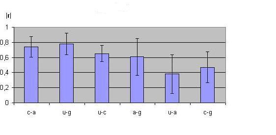
Figure 6: Specimen of invertebrates: Absolute value of the six highest correlation coefficient averaged over 8 a.a.. The error is computed by a standard deviation.

Figure 7: Specimen of invertebrates: absolute value of the six highest correlation coefficient averaged over 8 a.a.. correlation coefficient between codon frequency usage for quartets ending in (C,A),(U,G), (U,C) and (A,G). We do not report the correlations for quartets ending in (U,A) and (C,G), which are in general very low.

2.4.1 Test $\rho=0$ for INVERTEBRATES n=28

From eq.(5), we get that the critical value of the statistical label $t$ (95% confidence level) is

$${t_{c}=t_{5\%}^{n-2}=t_{0,025}^{26}=2,05}$$

• for $t_{r}\in[2,05;-2,05]$ the probability that $\rho=0$ (uncorrelated variables) is 95%.

• for $t_{r}>2,05\quad$or $\quad t_{r}<-2,05$ the probability that $\rho=0$ is 5%

In Tables 15 and 13 we report, respectively, the computed value of the $t$ label for any a.a. and the interval where the values of the correlation coefficient $r$ are included in, at 95 % confidence level.

$INV$	$r_{CA}$	$r_{UG}$	$r_{UC}$	$r_{AG}$	$r_{UA}$	$r_{CG}$
t[P]	-6,2	-4,1	-3,0	-5,6	1,0	3,1
t[T]	-8,2	-8,9	-5,6	-6,0	4,0	3,8
t[A]	-7,2	-6,6	-5,8	-4,7	3,1	3,2
t[S]	-10,9	-7,7	-5,1	-8,5	3,4	6,6
t[V]	-6,4	-11,8	-4,5	-6,3	5,3	2,7
t[L]	-2,9	-11,8	-2,8	-4,5	2,9	1,3
t[R]	-3,4	-6,0	-6,0	-1,4	0,0	3,2
t[G]	-5,5	-2,8	-3,6	-0,7	-0,1	0,4
$<t>_{a.a.}$	-6,34	-7,46	-4,55	-4,71	2,45	3,04

Table 15: Specimen of invertebrates: value of the statistical label $t$ for the 6 correlation coefficients for the 8 a.a.. In the last row the average value of $t$.

INV	$r_{CA}$	$r_{UG}$		$r_{UC}$	$r_{AG}$		$r_{UA}$	$r_{CG}$
P	-0,57 -0,89	-0,34 -0,81		-0,16 -0,74	-0,51 -0,87		-0,19 0,53	0,18 0,75
T	-0,70 -0,93	-0,74 -0,94		-0,51 -0,87	-0,54 -0,88		0,32 0,81	0,29 0,8
A	-0,64 -0,91	-0,59 -0,90		-0,52 -0,88	-0,41 -0,84		0,17 0,74	0,2 0,75
S	-0,81 -0,96	-0,66 -0,92		-0,46 -0,86	-0,72 -0,93		0,22 0,77	0,59 0,9
V	-0,57 -0,89	-0,83 -0,96		-0,38 -0,83	-0,57 -0,89		0,47 0,86	0,1 0,71
L	-0,14 -0,73	-0,83 -0,96		-0,13 -0,72	-0,38 -0,83		0,16 0,74	-0,14 0,57
R	-0,22 -0,77	-0,54 -0,88		-0,54 -0,88	0,11 -0,58		-0,38 0,36	0,2 0,75
G	-0,49 -0,87	-0,13 -0,72		-0,25 -0,78	0,25 -0,49		-0,39 0,36	-0,3 0,44

Table 16: Confidence Intervals (95% confidence level) for the specimen of invertebrates n=28

Figure 8: Value of $|t|$ for the correlation coefficients for the specimen of invertebrates.

From Table 15 we remark, also in this case, that the value of the modulus of the statistical label $t$ computed over the specimen of invertebrates is, in the average, more far from the critical value $t_{c}=2,05$ for the correlation $r_{CA}$ and $r_{UG}$ than for $r_{UC}$ and $r_{AG}$. From Table 16, one correlation factor can be vaninishing (95% confidence level) for the couple (A,G), i.e. Arg, three for the couple (U,A), i.e. Arg, Gly and Pro, and at least two for the couple (C,G), i.e. Leu and Gly.

2.5 Mitochondrial code

In Table 17 we report the correlations coefficient for the 6 independent couples of probabilities for the 8 quartets for the specimen of mitochondria of vertebrates, see Table 30.

$r_{XY}$	$r_{CA}$	$r_{UG}$		$r_{UC}$	$r_{AG}$		$r_{UA}$	$r_{CG}$
P	-0,78	0,28		-0,14	-0,22		-0,49	-0,12
T	-0,84	0,38		-0,33	0,02		-0,23	-0,32
A	-0,78	-0,16		-0,68	0,19		0,10	-0,21
S	-0,83	-0,15		-0,49	-0,74		-0,05	0,63
V	-0,59	-0,08		-0,44	-0,49		-0,41	0,26
L	-0,34	-0,22		-0,64	-0,21		-0,48	0,22
R	-0,70	-0,12		-0,18	-0,33		-0,32	-0,19
G	-0,69	0,57		-0,41	-0,39		-0,31	-0,29
$<r>_{a.a.}$	-0,69	0,06		-0,41	-0,27		-0,27	-0,02

Table 17: Mitochondria vertebrates:value of the correlation coefficient for the 6 independent couples of probabalities for the 8 quartets. In the last row the value of the coefficient averaged over the 8 a.a..

We remark that

• only the coefficient $r_{CA}$ for Pro, The, Ala and Ser has a relatively high value ($r\sim 0,8$), but the coefficient $r_{UG}$ for the complementary couple does not show this property. The other values do indicate the absence of correlation.

• the c.u.f. for mitochondria is more asymmetric that for eukaryotes. It seems the codons $XYA$ and $XYC$ are most used while the remaining codons, in particular $XYC$, are very poorly used.

In Fig.(9) one can remark that the codon frequency distribution on the 4 codons is more asymmetric than in the analogous figures for eukaryotic species The mitochondrial genetic information seems to be preferably encoded by codons XZA and XZC, the two remaining codons, in particular XZG, are for the most part little used or resolutely suppressed. In particular in Fig.(9) we remark,in correspondence of the quartets P,T,A,S ($r_{CA}\sim 0,8$), $P(XZG)\sim 0,05$ and $P(XZU)\sim 0,15$, so$P_{A+C}\approx 1-0,20=0,80$, as it is obtained by averaging over the 20 species.

2.5.1 Test $\rho=0$ for Mitochondres n=20

From eq.(5), we get that the critical value of the statistical label $t$ (95% confidence level) is

$${t_{c}=t_{5\%}^{n-2}=t_{0,025}^{18}=2,1}$$

• for $t_{r}\in[2,1;-2,1]$ the probability that $\rho=0$ (uncorrelated variables) is 95%.

• for $t_{r}>2,1\quad$ or $\quad t_{r}<-2,1$ the probability that $\rho=0$ is 5%

In the Table 18 we report the computed value of the $t$ label for any a.a. and we indicate in bold the values of the correlation coefficients for whch it is plausible to take the value $\rho=0$ (uncorrelated at 95% confidence level).

MIT	$r_{CA}$	$r_{UG}$	$r_{UC}$	$r_{AG}$	$r_{UA}$	$r_{CG}$
t[P]	-5,29	1,24	-0,60	-0,96	-2,38	-0,51
t[T]	-6,57	1,74	-1,48	0,08	-1,00	-1,43
t[A]	-5,29	-0,69	-3,93	0,82	0,43	-0,91
t[S]	-6,31	-0,64	-2,38	-4,67	-0,21	3,44
t[V]	-3,10	-0,34	-2,08	-2,38	-1,91	1,14
t[L]	-1,53	-0,96	-3,53	-0,91	-2,32	0,96
t[R]	-4,16	-0,51	-0,78	-1,48	-1,43	-0,82
t[G]	-4,04	2,94	-1,91	-1,8	-1,38	-1,29

Table 18: Mitochondria vertebrates: value of the statistical label $t$ for the 6 correlation coefficients for the 8 a.a..

A general survey of Table 18 confirms that the absence of any correlation is consistent with the obtained results.

Figure 9: Probability of the four codons in the 8 a.a. for the mitochondrial code.

Figure 10: Mitochondrial specimen: diagram of $|t|$.

Let us remark that the $|t|$ diagram for the mitochondrial specimen shows that most of the value of $|t|$ are below the critical value $t_{c}=2,1$.

3 Correlation between amino-acids

In [Frappat et al., 1999], [Chiusano et al., 2001] it was remarked that the values of the ratio

$$B_{NN^{\prime}}=\frac{P_{XYN}}{P_{X^{\prime}Y^{\prime}N^{\prime}}}$$ (8)

were independent on the considered biological species and, for any biological species, were very close each other for $XY,X^{\prime}Y^{\prime}\in\{CU,GU\}$ or $XY,X^{\prime}Y^{\prime}\in\{CC,UC,GC,AC\}$, i.e. for the quartets encoding, respectively, Leu, Val and Pro, Ser, Ala, Thr. This feature suggests the possible existence of a correlation between $P_{XYN}$ and $P_{X^{\prime}Y^{\prime}N}$ for $XY,X^{\prime}Y^{\prime}$ belonging to one of the two above specified sets. In order to search for correlation we computed the $28\times 28$ correlation matrix $r_{XYN,X^{\prime}Y^{\prime}N}\equiv r_{P_{XYN},P_{X^{\prime}Y^{\prime}N}}$ for the 8-dinucleotides corresponding to quartets. We do not report here the whole matrix, but the following interesting correlation pattern comes out

a.a.	XY-X’Y’	$r_{AA}$	$r_{CC}$	$r_{GG}$	$r_{UU}$
Ala-Pro	GC-CC	0,86	0,93	0,93	0,81
Ala-Ser	GC-UC	0,86	0,93	0,82	0,81
Ala-Thr	GC-AC	0,91	0,93	0,93	0,94
Pro-Ser	CC-UC	0,93	0,90	0,87	0,91
Pro-Thr	CC-AC	0.83	0,91	0.93	0.74
Ser-Thr	UC-AC	0.88	0,94	0.90	0.80
Leu-Val	CU-GU	0.85	0,82	-0.70	0.96

Table 19: Correlation between probabilities for codons in quartets encoding different amino acids computed over the whole eukariotes specimen $n=92$.

We should say that, in the 406 independent entries of the correlation matrix for the 8 quartets, several values larger than, let us say, 0.75 do appear, but only for the a.a. listed in Table 19 all the entries are, with exception of $r_{CUG,GUG}$, which further is the only negative values, equal or larger than 0.75. In order to get an evaluation of the effects of the statistics of the number of codons, as well as to increase the statistics of the analysed specimen, we have computed this correlation matrix over a specimen of $n=218$ biological species with a codons statistics larger than 30.000 codons. For the 6 a.a. Ala, Pro, Ser, Thr, Val and Leu, we extract the following correlation pattern reported in Table 20

a.a.	XY-X’Y’	$r_{AA}$	$r_{CC}$	$r_{GG}$	$r_{UU}$
Ala-Pro	GC-CC	0,73	0,89	0,91	0,74
Ala-Ser	GC-UC	0,86	0,85	0,79	0,80
Ala-Thr	GC-AC	0,77	0,87	0,91	0,85
Pro-Ser	CC-UC	0,82	0,82	0,85	0,82
Pro-Thr	CC-AC	0.74	0,80	0.91	0.73
Ser-Thr	UC-AC	0.80	0,87	0.88	0.79
Leu-Val	CU-GU	0.80	0,73	-0.61	0.94

Table 20: Correlation between probabilities for codons in quartets encoding different amino acids computed over a specimen of $n=218$ species with a codons statistics $\geq$ 30.000.

From a comparison of Table 19 and of Table 20 we see that the general pattern is unchanged, even if the values of the correlation coefficients are lower. Looking at these Tables it shows out that the set of eight quartes splits into three subsets

• a set of 4 a.a. (Pro, Ser, Ala, Thr) which shows a correlation between the c.u.f. for codon with the same third nucleotide

• a set of 2 a.a. (Leu, Val) which shows a correlation between the c.u.f. for codon with the same third nucleotide

• a set of 2 a.a. (Arg, Gly) (not reported in Table) with generally uncorrelated c.u.f.

This pattern fits well in the crystal basis model of the genetic code. Indeed in the model the codons belonging to the quartets encoding Pro, Ser, Ala, Thr are identified by elements of the same mathematical space; the same happens for the quartets encoding Leu, Va, while the remaining two quartes, encoding for Arg an Gly, do not share this feature.

4 Pattern of the Shannon entropy

The Shannon entropy, defined by

$$S=-\sum_{i}\,f_{i}\,\ln_{2}f_{i}$$ (9)

is largely used in biology, mainly to compute the distance between the observed frequencies $f_{i}$ of some quantity and the theoretically predicted ones. In [Frappat et al., 2005] it has been argued that the contribution of each quartet, in the total exonic region, to the Shannon entropy, defined as:

$$S_{XY}=-\sum_{N=C,A,U,G}p_{XYN}\,\ln_{2}p_{XYN}$$ (10)

should be independent on the biological species. Pay attention to not confuse the previous defined probability $P(XYN)\equiv P_{N}$ with the probability $p_{XYN}$ with the normalization condition

$$\sum_{X,Z,N\in C,A,U,G}\,p_{XZN}\,=\,1$$ (11)

A consequence of this statement is that biological species with the same percentage, in the total exonic decoded region, of a given a.a. should have the same Shannon entropy, computed by eq.(9). As we are dealing with a.a. encoded by quartets, the a.a. can be also identified by the first two nucleotides $XY$, so we should have

$$S_{XY}=-\sum_{N=C,A,U,G}p_{XYN}\,\ln_{2}p_{XYN}=-\sum_{N=C,A,U,G}\widehat{p}_{XYN}\,\ln_{2}\widehat{p}_{XYN}$$ (12)

where $p_{XYN}$ and $\widehat{p}_{XYN}$ are the codon usage frequencies for the quartet encoding the a.a. specified by the dinucledotide $XY$ for two different biological species with the condition

$$\sum_{N=C,A,U,G}p_{XYN}\,=\,\sum_{N=C,A,U,G}\widehat{p}_{XYN}\,\equiv\mbox{percentage of thw a.a. XY in the exonic decoded region}$$ (13)

In Table 21 and Table 22 we report, respectively, for a set of two and three different biological species, belonging to the considered specimen, which have approximately the same percentage of a given a.a. the computed Shannon entropy. The data confirm largely the independence of the value of the entropy from the values of $p_{XYN}$ peculiar of the considered b.sp.. However care must be used in concluding that the calculated Shannon entropy values satisfy eq.(13). Indeed one has to take into account that the values of $p_{XYN}$ are quite small (for the quartets $5\cdot 10^{-2}>p_{XYN}>2\cdot 10^{-3}$). So it is natural to wonder if one is really observing a property of the entropy or an artefact due to the smallness of the frequencies. In order to shed light on the question, we have made some simulations which confirm the validity of eq.(13). If one consider, e.g., the case of Thr, which appears in the coding region of Xenopus Laevis, Plasmodium vivax and Plasmodium patents, respectively, with percentage value 5,270 %,, 5,267 % and 5,279 %, see Table 22, changing of approximately 10 % the observed c.u.f., the value of the Shannon entropy is modified in the second decimal digit. In the average a change of the c.u.f. of the order of a standard deviation does not affect the third decimal digit. These considerations do not completely solve the above raised question, but give a cue the equality of the values of the Shannon entropy in Tables 21 and 22 to be an indication of this (unexpected) feature.

From the statement of eq.(12) it follows that the knowledge of the c.u.f., typical of a fixed biological species, does not provide further information on the Shannon entropy of the a.a., i.e. the knowledge of the four quantities $p_{XYN}$, constrained by the condition eq.(13) gives the same amount of information of the knowledge of only one quantity $\{XY\}(\equiv$ percentage of the a.a. XY). This is understandable, on general grounds, if the four $p_{XYN}$ are constrained by two further constraints, which may be the correlations, respectively, between $p_{XYC}$ and $p_{XYA}$ and between $p_{XYG}$ and $p_{XYU}$. That being the case the knowledge of the four $p_{XYN}$ in fact reduces to the knowledge of only one independent quantity equivalent to the knowledge of $\{XY\}$. So the computation of the Shannon entropy provides a further support to the existence of the correlations.

a.a.	b.sp.	b.sp.		% 1st-col	2nd-col		$S_{1}(a.a.)$	$S_{2}(a.a.)$
Ala	15	34		8,425	8,421		0,467	0,464
	1	26		7,166	7,167		0,41	0,398
	23	19		6,866	6,868		0,392	0,385
	23	29		5,619	5,611		0,329	0,339
Arg	19	38		3,368	3,369		0,228	0,228
	26	5		3,246	3,247		0,221	0,222
	14	5		3,245	3,247		0,223	0,222
	12	15		3,133	3,134		0,217	0,215
	11	17		3,085	3,092		0,215	0,213
	3	6		3,057	3,066		0,213	0,212
	13	29		1,377	1,38		0,111	0,11
Gly	25	23		7,835	7,835		0,44	0,44
	3	38		7,311	7,299		0,415	0,415
	4	28		7,199	7,195		0,416	0,41
	9	26		7,162	7,164		0,391	0,404
	8	35		6,393	6,397		0,38	0,365
	18	27		5,449	5,442		0,329	0,323
Leu	2	17		7,496	7,499		0,396	0,42
	13	38		7,424	7,426		0,406	0,417
	15	2		7,247	7,249		0,413	0,411
	1	3		7,068	7,064		0,39	0,401
	4	22		5,607	5,608		0,34	0,339
Pro	16	5		6,126	6,125		0,364	0,364
	13	5		6,123	6,125		0,364	0,364
	5	24		5,714	5,715		0,348	0,346
	23	12		5,491	5,497		0,334	0,334
	26	37		5,44	5,439		0,336	0,326
	4	18		5,149	5,15		0,317	0,323
	1	25		5,028	5,032		0,315	0,317
	4	6		4,901	4,909		0,295	0,299
Ser	18	9		6,077	6,067		0,366	0,36
	7	8		5,109	5,109		0,314	0,315
	24	27		5,09	5,098		0,319	0,302
	3	15		5,041	5,041		0,318	0,311
	2	27		5,033	5,027		0,313	0,317
	12	33		5	5,003		0,309	0,315
	18	13		4,984	4,989		0,306	0,314
	15	14		4,747	4,744		0,297	0,267
	15	19		4,747	4,744		0,297	0,287
	26	17		4,368	4,369		0,278	0,284
Thr	3	36		5,826	5,822		0,355	0,342
	2	9		5,774	5,774		0,341	0,345
	16	35		5,774	5,77		0,344	0,348
	11	26		5,684	5,683		0,342	0,348
	7	26		5,687	5,683		0,347	0,348
	11	7		5,684	5,687		0,342	0,347
	1	26		5,479	5,474		0,331	0,329
	10	26		5,479	5,474		0,331	0,329
	7	1		5,389	5,384		0,327	0,331
	16	16		5,309	5,307		0,326	0,325
	17	10		5,289	5,282		0,324	0,31
	24	25		5,278	5,279		0,324	0,329
	25	22		5,27	5,267		0,32	0,328
	25	18		5,109	5,11		0,297	0,317
	19	15		5,059	5,056		0,298	0,312
Val	17	25		7,224	7,228		0,413	0,408
	16	17		7,011	7,017		0,384	0,397
	1	10		6,9	6,925		0,392	0,357
	19	18		6,715	6,719		0,376	0,388
	4	37		6,701	6,705		0,381	0,382
	25	2		6,601	6,607		0,369	0,378
	13	28		6,017	6,016		0,352	0,354
	22	12		6,091	6,08		0,351	0,363
	17	21		5,954	5,958		0,355	0,352

Table 21: In the first column it is indicated the a.a.. In the second and third column the number identifies the species denoted for vertebrates (bold font, x), for plants (normal font, x) and for invertebrates (italic font, x). In the next two columns the percentage of the a.a. and In the last two columns the computed Shamnon entropy relative to the a.a.. for the biological species specified in the 2nd anf 3rd column.

a.a.	VRT	INV	PLN	% a.a. V	% a.a. I	% a.a. I	$S^{a.a.}$ V	$S^{a.a.}$ I	$S^{a.a.}$ P
Ala	3	1	26	7,156	7,166	7,167	0,41	0,41	0,398
	13	22	15	7,025	7,084	7,115	0,40	0,407	0,402
	9	18	32	6,767	6,74	6,808	0,388	0,396	0,382
	7	10	30	7,344	6,336	6,262	0,369	0,367	0,361
Arg	19	3	38	3,368	3.347	3,369	0,228	0,229	0,222
	16	4	18	3,286	3,313	3,273	0,225	0,225	0,222
	25	5	30	3,264	3,247	3,267	0,224	0,222	0,219
	12	15	17	3,133	3,134	3,092	0,217	0,215	0,213
	22	24	34	2,841	2,871	2,806	0,201	0,203	0,196
Gly	21	28	20	7,159	7,160	7,165	0,412	0,412	0,402
	20	28	12	7,139	7,160	7,130	0,411	0,412	0,411
	26	10	22	6,842	6,821	6,807	0,397	0,384	0,394
	24	15	22	6,713	6,739	6,807	0,389	0,394	0,394
	5	27	22	6,702	6,701	6,807	0,392	0,393	0,394
	18	14	1	6,609	6,511	6,581	0,388	0,332	0,382
	14	13	1	6,548	6,505	6,583	0,386	0,374	0,382
	3	1	11	6,457	6,497	6,474	0,383	0,377	0,378
	17	23	2	6,038	5,993	5,937	0,364	0,345	0,355
Leu	17	2	17	7,506	7,496	7,499	0,417	0,396	0,42
	5	9	37	7,443	7,453	7,459	0,401	0,382	0,41
	8	8	28	6,876	6,93	6,943	0,393	0,383	0,391
Pro	25	16	35	5,905	5,885	5,863	0,354	0,348	0,356
	5	24	38	5,714	5,715	5,554	0,348	0,346	0,343
	1	4	19	4,894	4,901	4,909	0,308	0,297	0,299
Ser	13	11	22	5,359	5,419	5,409	0,274	0,325	0,328
	7	8	25	5,109	5,109	5,126	0,314	0,315	0,322
	5	24	27	5,105	5,09	5,098	0,313	0,319	0,302
	2	3	15	5,033	5,041	5,041	0,313	0,318	0,311
	2	27	15	5,033	5,027	5,041	0,313	0,317	0,311
	12	27	33	5	5,027	5,003	0,309	0,314	0,315
	17	25	34	4,917	4,875	4,888	0,304	0,267	0,309
	15	14	17	4,747	4,744	4,736	0,297	0,287	0,301
	24	9	18	4,292	4,169	4,239	0,274	0,265	0,276
Thr	13	23	21	5,982	6,018	6,03	0,357	0,346	0,359
	11	26	7	5,684	5,683	5,687	0,342	0,348	0,347
	7	1	24	5,389	5,384	5,411	0,327	0,331	0,331
	24	22	25	5,278	5,267	5,279	0,324	0,328	0,329
	25	22	25	5,27	5,267	5,279	0,324	0,328	0,329
Val	1	16	10	6,9	7,011	6,925	0,392	0,384	0,357
	25	2	22	6,601	6,607	6,604	0,369	0,378	0,384
	18	14	34	6,573	6,566	6,588	0,372	0,348	0,38
	16	24	12	6,099	6,137	6,08	0,357	0,368	0,363
	17	8	21	5,954	5,895	5,958	0,355	0,347	0,352

Table 22: In the first column it is indicated the a.a.. In the second, third, fourth column the number identifies the species, respectively, for vertebrates (V), plants (P) and invertebrates (I). In the next three columns and, respectively, in the last three the percentage of the a.a. and the computed Shamnon entropy, for the indicated biological species, columns.

5 Conclusions

We can summarize the results as it follows

• Eucaryotes: for all a.a., the variance reduction for the probabilities $P_{U+G}$ and $P_{C+A}$ is larger than the reduction for the values of $P_{U+C}$, $P_{A+G}$, $P_{C+G}$ and $P_{U+G}$ while the value of the ratio $\sigma^{2}_{mis}/\sigma^{2}_{th}$ is close to one for $P_{C+G}$ and $P_{U+G}$, see Table 23.

  Prob.	$\small{<{\sigma_{obs}}^{2}/{\sigma_{th}}^{2}>_{a.a}^{\texttt{VRT}}}$	$\small{<{\sigma_{obs}}^{2}/{\sigma_{th}}^{2}>_{a.a}^{\texttt{INV}}}$	$\small{<{\sigma_{obs}}^{2}/{\sigma_{th}}^{2}>_{a.a}^{\texttt{PLN}}}$
  $P_{C+A}$	0,14	0,28	0,21
  $P_{U+G}$	0,22	0,27	0,26
  $P_{U+C}$	0,31	0,38	0,33
  $P_{A+G}$	0,42	0,44	0,50
  $P_{U+A}$	1,69	1,36	0,50
  $P_{C+G}$	1,36	1,44	1,50

  Table 23: Value of the ratio $\sigma^{2}_{obs}(X+Y)$ and ${\sigma^{2}}_{th}(X+Y)\equiv\sigma^{2}_{obs}(X)+\sigma^{2}_{obs}(Y)$ averaged over the 8 aminoacids - $<\sigma^{2}/{\sigma_{th}}^{2}>_{a.a}$ - for sum of the probabilities.

  In more detail:

  1. Vertebrates: from Table 7 the ratio $\sigma^{2}/{\sigma^{2}}_{th}$ is smaller for $C+A$ than for $U+G$ for all a.a., except Arg (R), Leu (L) and Val (V) for which the contrary is true.
     In the average, for the 8 a.a. encoded by quartets we find:

     1. For $P_{C+A}$ for $P_{U+G}$ $\sigma^{2}\simeq 0,015-0,25\;{\sigma^{2}}_{th}$ . So, in the average, the variance reduction is approximately of one order of magnitude.

     2. For $P_{U+C}$ and $P_{A+G}$ $\sigma^{2}\simeq 0,3-0,40\;{\sigma^{2}}_{th}$

     3. For $P_{U+A}$ and $P_{C+G}$ $\sigma^{2}\simeq 1.4-1.7\;{\sigma^{2}}_{th}$.

  2. Invertebrates: from Table 7 the ratio $\sigma^{2}/{\sigma^{2}}_{th}$ is smaller for $U+G$ than for $C+A$ for all a.a except Ser (S), Pro (P) and Ala (A) or which the contrary is true.
     In the average, for the 8 a.a. encoded by quartets we find:

     1. For $P_{C+A}$ and $P_{U+G}$ $\sigma^{2}\simeq 0,3\;{\sigma^{2}}_{th}$ f.

     2. For $P_{U+C}$ and $P_{A+G}$, $\sigma^{2}\simeq 0,40-0,45\;{\sigma^{2}}_{th}$

     3. For $P_{U+A}$ and $P_{C+G}$ $\sigma^{2}\simeq 1.4\;{\sigma^{2}}_{th}$.

  3. Piantes: from Table 7 the ratio $\sigma^{2}/{\sigma^{2}}_{th}$ is smaller for $C+A$ than for $U+G$ for all a.a except Leu (L) and Val (V) for which the contrary is true.
     In the average, for the 8 a.a. encoded by quartets we find:

     1. For $P_{C+A}$ and $P_{U+G}$.$\sigma^{2}\simeq 0,20-0,25\;{\sigma^{2}}_{th}$

     2. For $P_{U+C}$ and $P_{A+G}$ $\sigma^{2}\simeq 0,30-0,50\,{\sigma^{2}}_{th}$

     3. For $P_{U+A}$ and $P_{C+G}$ $\sigma^{2}\simeq 1.4-15\;{\sigma^{2}}_{th}$.

  In conclusion a pattern comes out in which, for the three considered specimens the variance reduction for the couples $A,C$ and $U,G$ is larger than for the other couples, as it can be inferred by Tables 3 and 3 where the average values of $P_{C}$, $P_{A}$, $P_{C+A}$. and, respectively, of $P_{G}$, $P_{U}$ and $P_{G+U}$ are reported .

• Mitochondria

  The variance reduction seems appeciable only for the couple $C+A$ for which, in the average, $\sigma^{2}/{\sigma^{2}}_{th}\sim 0,3$, while for the remaining couples $\sigma^{2}/{\sigma^{2}}_{th}\geq 0,6$.

So no clear cue for the existence of correlation in c.u.f. for Mitochondria comes out from the previous analysis.

In [Frappat et al., 2003] a theoretical correlation matrix has been derived from the sum rule for the sum the probabilities of the synonimous codons in quartes with last nucleotide $C$ and $A$., which we compare, in Table 24 with the computed one for the three eukaryotic specimen. The theoretical value are indicated in round brackets in the first column, $x$ is a not a priori computable entry.

	VRT	PLN	INV
$<r_{CA}>_{a.a.}$ ( -1)	-0.89	- 0.83	-0.74
$<r_{UG}>_{a.a}({\color[rgb]{1,0,0}-1})$	-0.80	-0.78	–0.78
$<r_{UC}>_{a.a}$ ( -x)	-0.76	-0.69	-0.65
$<r_{AG}>_{a.a}$ ( -x)	-0.64	-0.55	-0.61
$<r_{UA}>_{a.a}$ ( x)	0.74	0.53	0.38
$<r_{CG}>_{a.a}$ ( x)	0.41	0.37	0.47

Table 24: Observed averaged value for the correlation matrix, in bracket the theoretical value.

Table 24 shows that the computed values of $<r_{NN^{\prime}}>$ differ from the theoretical ones by a quantity of the value of 10-15 %, excepr for $<r_{CG}>$ and, for the specimen of invertebrates, for $<r_{UA}>$. For $<r_{CG}>$ the anomalous behaviour may be understood from the known suppression of the dinucleotide $CG$, see for possible explanation of the suppressione [Knight et al., 2001], [Klump and Maeder, 1991]. In conclusion one remarks that there is a strong indication for the existence of correlation between $P_{C}$ and $P_{A}$ (respectively$P_{G}$ and $P_{U}$), which further is unexpectedly high for the specimen of plants. Indeed while one can argue that vertebrates are ”similar” species in the phylogenetic tree, plants are an extremely large domain of species. The correlation is less evident for invertebrates, but one should keep in mind that this is not even a domain in the life world, May be one should look for correlations in suitable subsets of invertebrates. It comes out that the ratio of $\sigma_{P_{C+A}}$ over $<P_{C+A}>$ is in the range of 0,02-0,05 for vertebrates, 0,11-0,26 fo plants, 0,09-0,20 for invertebrates. These last two results rise serious question on the validity of the sum rule, still in presence of a clear indication of correlation.

There are several directions which seem worthwhile to be investigated:

• further statistical analysis with better statistics and further tests of the reliability of the presence of the correlations

• the main reasons for the codon usage bias are believed to be: the mutational bias, the translation efficiency, the selection mechanism and the abundance of specific anticodons in the tRNA. The universal presence of correlations suggests that its origin may lie in some very general mechanisms, possibly related to the structure of the genetic code. It seems worthwhile to search for mutation-selection models able to explain the pattern of the correlation. Work is in progess in this direction.

• further statistical analysis of the behaviour of the Shannon entropy to further test the validity of eq.(12).

Let us emphasize our claim: we have remarked that the sum of the usage probabilities of two suitably choosen codons is, within a few percent, a constant independent on the biological species for vertebrates, which well fits in the framework of the crystal basis model. Of course one can restate the above results stating the sum of the probability of codon usage $XZC+XZA$ is not depending on the nature of the biological specie, without any reference to crystal basis model. However a deeper analysis of Table 31 shows that $P_{C+A}$ for Pro, Thr, Ala, Ser and Gly is of the order of 0.62, for Leu and Val of the order 0.35 while for Arg is of order 0.52. In the crystal basis model the roots, i.e. the dinucleotide formed by the first two nucleotides of the first 5 amino acids belong to the same irrep. (1,1), the roots of Leu and Val belong to the irrep. (0,1), while the root of Arg belongs to the irrep. (1,0). This is an interesting result, especially for Pro whose molecule has a different structure than the others amino acids (Pro has an imino group instead of an amino group).

It is natural to wonder what happens for other biological species. The green plants exhibits roughly the same pattern, but probably a more reliable analysis has to be performed considering a splitting into families. For invertebrates, the large number of existing biological species and the lack of data with sufficient diversity prevents from applying a similar analysis. The case of bacteriae is rather interesting. Eubacteriae seem to avoid this pattern of correlations. This may be the influence of selection effects which may be stronger or effective in shorter times in less complicated species. For bacteriae the G+C content varies in a wide range from 25 % to 75 %. Hence one can argue that biological species with large difference in the G+C content exhibit large difference in the correlation pattern discussed in this paper. However, using the Genbank data, one finds for eubacteriae no correlation between the G+C content and the value of the probabilities eq.(23).

Acknowledgments It is a pleasure to thank M. Nicodemi for discussions and useful suggestions.

6 Appendix

6.1 The crystal basis model of the genetic code

For completeness let us briefly recall the main features of the crystal basis model of the genetic code. Each codon $XZN$ is described by a state belonging to an irreducible representation (irrep.), denoted $(J_{H},J_{V})^{\xi}$, of the algebra $U_{q}\big{(}sl(2)_{H}\oplus sl(2)_{V}\big{)}$ in the limit $q\to 0$ (so-called crystal basis); $J_{H}$, $J_{V}$ take (half-)integer values and the upper label $\xi$ removes the degeneracy when the same couple of values of $J_{H}$, $J_{V}$ appears several times. As can be seen in Table 26 there are for example four representations $({\textstyle{\frac{1}{2}}},{\textstyle{\frac{1}{2}}})^{\xi}$, with $\xi=1,2,3,4$. Within a given representation $(J_{H},J_{V})^{\xi}$ two more quantum numbers $J_{H,3}$, $J_{V,3}$ are necessary to specify a particular state. see Table 26, which is reported here to make the paper self-consistent.

in the model, it appears natural to write the codonusage probability as a function of the biological species (b.s.), of the particular amino-acid and of the labels $J_{H}$, $J_{V}$, $J_{H,3}$, $J_{V,3}$ describing the state $XZN$. Assuming the dependence of the amino-acid completely determined by the set of labels $J^{\prime}s$, we write

$$P(XZN)=P(b.s.;J_{H},J_{V},J_{H,3},J_{V,3})$$ (14)

With the further hypothesis that the r.h.s. of eq. (14) can be written as the sum of two contributions: a universal function $\rho$ independent on the biological species and a b.s. depending function $f_{bs}$, in [Frappat et al., 2005] the following equation has been written

$$P(XZN)=\rho^{XZ}(J_{H},J_{V},J_{H,3},J_{V,3})\;+\;f_{bs}^{XZ}(J_{H},J_{V},J_{H,3},J_{V,3})$$ (15)

Previous analysis, see [Chiusano et al., 2001], suggests the contribution of $f_{bs}$ is not negligible but smaller than the one due to $\rho$. So the following form form was assumed

$$f_{bs}^{XZ}(J_{H},J_{V},J_{H,3},J_{V,3})\approx F_{bs}^{XZ}(J_{H};J_{H,3})\,+\,G_{bs}^{XZ}(J_{V};J_{V,3})$$ (16)

In the framework of the model and of the above assumptions, the codon usage frequencies for the quartets Ala, Gly, Pro, Thr and Val and for the quartet sub-part of the sextets Arg (i.e. the codons of the form CGN), Leu (i.e. CUN) and Ser (i.e. UCN). was analysed.
For Thr, Pro, Ala and Ser one writes using Table 26 and eqs. (14)-(16), with $N=A,C,G,U$,

$$P(NCC)+P(NCA)=\rho_{C+A}^{NC}+F_{bs}^{NC}({\textstyle{\frac{3}{2}}};x)+G_{bs}^{NC}({\textstyle{\frac{3}{2}}};y)+F_{bs}^{NC}({\textstyle{\frac{1}{2}}};x^{\prime})+G_{bs}^{NC}({\textstyle{\frac{1}{2}}};y^{\prime})$$ (17)

$$P(NCG)+P(NCU)=\rho_{G+U}^{NC}+F_{bs}^{NC}({\textstyle{\frac{3}{2}}};x)+G_{bs}^{NC}({\textstyle{\frac{3}{2}}};y)+F_{bs}^{NC}({\textstyle{\frac{1}{2}}};x^{\prime})+G_{bs}^{NC}({\textstyle{\frac{1}{2}}};y^{\prime})$$ (18)

where $\rho_{C+A}^{NC}$ denotes the sum of the contribution of the universal function (i.e. not depending on the biological species) $\rho$ relative to $NCC$ and $NCA$, while the labels $x,y,x^{\prime},y^{\prime}$ depend on the nature of the first two nucleotides $NC$, see Table 26 in [Frappat et al., 2005]. Using the results of Table 26, One remarks that the difference between eq. (17) and eq. (18) is a quantity independent of the biological species,

$$P(NCC)+P(NCA)-P(NCG)-P(NCU)\;=\;\rho_{C+A}^{NC}-\rho_{G+U}^{NC}\;=\;\mbox{Const.}$$ (19)

In the same way, considering the cases of Leu, Val, Arg and Gly, we obtain with $W=C,G$

$$P(WUC)+P(WUA)-P(WUG)-P(WUU) = \rho_{C+A}^{WU}-\rho_{G+U}^{WU}\;=\;\mbox{Const.}$$ (20)

$$P(CGC)+P(CGA)-P(CGG)-P(CGU) = \rho_{C+A}^{CG}-\rho_{G+U}^{CG}\;=\;\mbox{Const.}$$ (21)

$$P(GGC)+P(GGA)-P(GGG)-P(GGU) = \rho_{C+A}^{GG}-\rho_{G+U}^{GG}\;=\;\mbox{Const.}$$ (22)

Since the probabilities for one quadruplet are normalised to one, from eqs. (18)-(22) we deduce that for all the eight amino acids the sum of probabilities of codon usage for codons with last A and C (or U and G) nucleotide is independent of the biological species, i.e.

$$P(XZC)+P(XZA)=\mbox{Const.}\qquad(XZ=NC,CU,GU,CG,GG)$$ (23)

Now let us make two important remarks.
– If we write for $\rho(J_{H},J_{V},J_{H,3},J_{V,3})$, or equivalently $\rho_{C+A}^{NC}$, an expression of the type (16), i.e. separating the $H$ from the $V$ dependence, it follows that the r.h.s. of eqs. (17) and (18) are equal, and consequently the probabilities $P(NCC)+P(NCA)$ and $P(NCU)+P(NCG)$ should be equal, which is not experimentally verified. This means that the coupling term between the $H$ and the $V$ is not negligible for the $\rho(J_{H},J_{V},J_{H,3},J_{V,3})$ function.
– Summing equations (17) and (18) we deduce that the expression $F_{bs}^{NC}({\textstyle{\frac{3}{2}}};x)+G_{bs}^{NC}({\textstyle{\frac{3}{2}}};y)+F_{bs}^{NC}({\textstyle{\frac{1}{2}}};x^{\prime})+G_{bs}^{NC}({\textstyle{\frac{1}{2}}};y^{\prime})$ is actually not depending on the biological species. From eqs. (17) and (18) for different values of $N$ and for analogous equations for the other four quartets, we can derive relations between sums of $F_{bs}^{NC}$ and/or $G_{bs}^{NC}$ functions which are independent of the biological species.

6.2 Statistical analysis

In the following we recall, for completeness, the definition of the statistical quantities used in the text:

• the standard deviation

  $$\sigma_{P}=\sqrt{\frac{1}{n(n-1)}(n\sum_{i=1}^{n}P_{i}^{2})-(\sum_{i=1}^{n}P_{i})^{2}}$$ (24)

  where $P_{N}$ is defined in eq.(4)

• the adimensional correlation coefficient $r_{XY}$

  $$r_{XY}=r_{(X_{1}.....X_{n};Y_{1}.....Y_{n})}=\frac{Cov(X,Y)}{\sigma_{X}\sigma_{Y}}$$

  $$=\frac{1}{\sigma_{X}\sigma_{Y}}\sum_{i=1}^{n}\frac{1}{n}(X_{i}-<X>)(Y_{i}-<Y>)\in[-1,1]$$ (25)

  where $<X>\>(<Y>)$ is the average value of the variable and $\sigma_{X}\>(\sigma_{Y})$ the corresponding standard deviation.

For two independent normally distributed variables $X$ and $Y$ we have

$$\sigma_{th}^{2}(X+Y)=\sigma^{2}(X)+\sigma^{2}(Y)$$ (26)

If $X\equiv P_{N}$ and $Y\equiv P_{N^{\prime}}$ we expect the value of the standard deviation of the sum of $X+Y$ to be smaller than the sum of the two corresponding standard deviation, due to the normalization condition

$\sum_{N=A,C,G,U}P_{N}=P(A)+P(C)+P(G)+P(U)=1$      ($P_{N+N}\equiv P_{N}+P_{N^{\prime}}$)

$$\sigma^{2}(P_{N+N^{\prime}})<\sigma^{2}(P_{N})+\sigma^{2}(P_{N^{\prime}})$$ (27)

However we expect the reduction to be approximately equal for any couple $P_{N}$ and $P_{N^{\prime}}$ extracted in the set of the four probabilities {$P(A)$,$P(C$),$P(G)$,$P(U)$}, while we remark that a reduction of the standard deviation for the sum $P_{A}+P_{C}$ and $P_{U}+P_{G}$ larger than for the other couples of probabilities. We can summarize the results as it follows ($\sigma_{th}^{2}(P_{N+N^{\prime}})=\sigma^{2}(P_{N})+\sigma^{2}(P_{N^{\prime}}$))

	XZU	XZC	XZA	XZG
XZU	1	-x	x	-1
XZC	-x	1	-1	x
XZA	x	-1	1	-x
XZG	-1	x	-x	1

Table 25: Correlation matrix for the codon probability from the sum rules (XZ = AC, CC, GC, UC, CU, GU, CG, GG).

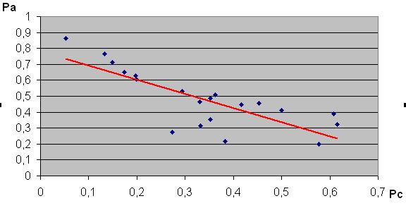
Figure 11: Grafico di correlazione per le frequenze d’uso dei codoni, misurate sul campione di mitocondri, terminanti per A e C dei quartetti (dall’alto in basso) ACN (Treonina), CCN (Proplina), GCN (Alalanina), UCN (Serina)

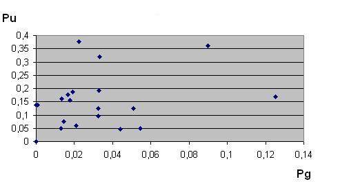
Figure 12: Graphic of the codon usage frequency $P_{U}$ versus $P_{G}$ for species belonging to the mitochondrial specimen. From top to bottom Thr, Pro, Ala and Ser CC

Table 26: The eukaryotic or standard code code. The upper label denotes different irreducible representations.

codon	amino acid	$J_{H}$	$J_{V}$	$J_{3,H}$	$J_{3,V}$	codon	amino acid	$J_{H}$	$J_{V}$	$J_{H,3}$	$J_{V,3}$
CCC	Pro P	$3/2$	$3/2$	$3/2$	$3/2$	UCC	Ser S	$3/2$	$3/2$	$1/2$	$3/2$
CCU	Pro P	$(1/2$	$3/2)^{1}$	$1/2$	$3/2$	UCU	Ser S	$(1/2$	$3/2)^{1}$	$-1/2$	$3/2$
CCG	Pro P	$(3/2$	$1/2)^{1}$	$3/2$	$1/2$	UCG	Ser S	$(3/2$	$1/2)^{1}$	$1/2$	$1/2$
CCA	Pro P	$(1/2$	$1/2)^{1}$	$1/2$	$1/2$	UCA	Ser S	$(1/2$	$1/2)^{1}$	$-1/2$	$1/2$
CUC	Leu L	$(1/2$	$3/2)^{2}$	$1/2$	$3/2$	UUC	Phe F	$3/2$	$3/2$	$-1/2$	$3/2$
CUU	Leu L	$(1/2$	$3/2)^{2}$	$-1/2$	$3/2$	UUU	Phe F	$3/2$	$3/2$	$-3/2$	$3/2$
CUG	Leu L	$(1/2$	$1/2)^{3}$	$1/2$	$1/2$	UUG	Leu L	$(3/2$	$1/2)^{1}$	$-1/2$	$1/2$
CUA	Leu L	$(1/2$	$1/2)^{3}$	$-1/2$	$1/2$	UUA	Leu L	$(3/2$	$1/2)^{1}$	$-3/2$	$1/2$
CGC	Arg R	$(3/2$	$1/2)^{2}$	$3/2$	$1/2$	UGC	Cys C	$(3/2$	$1/2)^{2}$	$1/2$	$1/2$
CGU	Arg R	$(1/2$	$1/2)^{2}$	$1/2$	$1/2$	UGU	Cys C	$(1/2$	$1/2)^{2}$	$-1/2$	$1/2$
CGG	Arg R	$(3/2$	$1/2)^{2}$	$3/2$	$-1/2$	UGG	Trp W	$(3/2$	$1/2)^{2}$	$1/2$	$-1/2$
CGA	Arg R	$(1/2$	$1/2)^{2}$	$1/2$	$-1/2$	UGA	Ter	$(1/2$	$1/2)^{2}$	$-1/2$	$-1/2$
CAC	His H	$(1/2$	$1/2)^{4}$	$1/2$	$1/2$	UAC	Tyr Y	$(3/2$	$1/2)^{2}$	$-1/2$	$1/2$
CAU	His H	$(1/2$	$1/2)^{4}$	$-1/2$	$1/2$	UAU	Tyr Y	$(3/2$	$1/2)^{2}$	$-3/2$	$1/2$
CAG	Gln Q	$(1/2$	$1/2)^{4}$	$1/2$	$-1/2$	UAG	Ter	$(3/2$	$1/2)^{2}$	$-1/2$	$-1/2$
CAA	Gln Q	$(1/2$	$1/2)^{4}$	$-1/2$	$-1/2$	UAA	Ter	$(3/2$	$1/2)^{2}$	$-3/2$	$-1/2$
GCC	Ala A	$3/2$	$3/2$	$3/2$	$1/2$	ACC	Thr T	$3/2$	$3/2$	$1/2$	$1/2$
GCU	Ala A	$(1/2$	$3/2)^{1}$	$1/2$	$1/2$	ACU	Thr T	$(1/2$	$3/2)^{1}$	$-1/2$	$1/2$
GCG	Ala A	$(3/2$	$1/2)^{1}$	$3/2$	$-1/2$	ACG	Thr T	$(3/2$	$1/2)^{1}$	$1/2$	$-1/2$
GCA	Ala A	$(1/2$	$1/2)^{1}$	$1/2$	$-1/2$	ACA	Thr T	$(1/2$	$1/2)^{1}$	$-1/2$	$-1/2$
GUC	Val V	$(1/2$	$3/2)^{2}$	$1/2$	$1/2$	AUC	Ile I	$3/2$	$3/2$	$-1/2$	$1/2$
GUU	Val V	$(1/2$	$3/2)^{2}$	$-1/2$	$1/2$	AUU	Ile I	$3/2$	$3/2$	$-3/2$	$1/2$
GUG	Val V	$(1/2$	$1/2)^{3}$	$1/2$	$-1/2$	AUG	Met M	$(3/2$	$1/2)^{1}$	$-1/2$	$-1/2$
GUA	Val V	$(1/2$	$1/2)^{3}$	$-1/2$	$-1/2$	AUA	Ile I	$(3/2$	$1/2)^{1}$	$-3/2$	$-1/2$
GGC	Gly G	$3/2$	$3/2$	$3/2$	$-1/2$	AGC	Ser S	$3/2$	$3/2$	$1/2$	$-1/2$
GGU	Gly G	$(1/2$	$3/2)^{1}$	$1/2$	$-1/2$	AGU	Ser S	$(1/2$	$3/2)^{1}$	$-1/2$	$-1/2$
GGG	Gly G	$3/2$	$3/2$	$3/2$	$-3/2$	AGG	Arg R	$3/2$	$3/2$	$1/2$	$-3/2$
GGA	Gly G	$(1/2$	$3/2)^{1}$	$1/2$	$-3/2$	AGA	Arg R	$(1/2$	$3/2)^{1}$	$-1/2$	$-3/2$
GAC	Asp D	$(1/2$	$3/2)^{2}$	$1/2$	$-1/2$	AAC	Asn N	$3/2$	$3/2$	$-1/2$	$-1/2$
GAU	Asp D	$(1/2$	$3/2)^{2}$	$-1/2$	$-1/2$	AAU	Asn N	$3/2$	$3/2$	$-3/2$	$-1/2$
GAG	Glu E	$(1/2$	$3/2)^{2}$	$1/2$	$-3/2$	AAG	Lys K	$3/2$	$3/2$	$-1/2$	$-3/2$
GAA	Glu E	$(1/2$	$3/2)^{2}$	$-1/2$	$-3/2$	AAA	Lys K	$3/2$	$3/2$	$-3/2$	$-3/2$

Table 27: Data for vertebrates from GenBank [Release 149.0]

	Biological species	number of sequences	number of codons	GC %
1	Bos taurus	3526	1434728	53,81
2	Canis familiaris	948	443570	53,29
3	Cavia porcellus	388	159307	52,07
4	Cricetulus griseus	302	142938	51,02
5	Cyprinus carpio	344	137658	49,89
6	Danio rerio	12639	5184976	50,55
7	Equus caballus	317	115073	52,92
8	Felis catus	282	108779	52,54
9	Gallus gallus	5498	2507341	51,21
10	Homo sapiens	82409	35354305	52,41
11	Macaca fascicularis	4029	1403004	49,17
12	Macaca mulatta	683	224889	52,84
13	Mesocricetulus auratus	301	128917	52,56
14	Mus musculus	39535	18330339	52,26
15	Mus sp.	573	124703	52,77
16	Oncorhynchus mykiss	725	271803	53,25
17	Oryctolagus cuniculus	1038	506266	54,7
18	Oryzias latipes	434	193442	52,32
19	Ovis aries	597	188842	53,48
20	Pan troglodytes	272	281194	54,41
21	Rattus norvegicus	13977	6477319	52,59
22	Rattus sp.	654	127597	52,37
23	Sus scrofa	1932	758646	54,25
24	Takifugu rubripes	746	363990	54,61
25	Xenopus laevis	10831	4760901	46,88
26	Xenopus tropicalis	3080	1181338	47,8

Table 28: Data for invertebrates from GenBank [Release 149.0]

	Biological species	number of sequences	number of codons	GC %
1	Aedes aegyptiana	454	198039	50,52
2	Anopheles gambiae	578	248920	55,89
3	Bombyx mori	751	300663	48,71
4	Caenorhabditis elegans	24353	10911983	42,93
5	Ciona intestinalis	726	356806	45,18
6	Cryptosporidium parvum	638	400196	33,28
7	Dictyostelium discoideum	3349	1953700	28,63
8	Drosophila melanogaster	38522	20352622	53,89
9	Drosophila pseudoobscura	301	107621	54,85
10	Drosophila simulans	609	214015	52,59
11	Drosophila subobscura	291	107270	55,64
12	Drosophila virilis	214	114895	53,52
13	Encephalitozoon cuniculi GB-M11	1995	718636	47,52
14	Entamoeba histolytica 6 285	115735	31,38
15	Giardia intestinalis	355	178606	52,02
16	Leishmania major	1714	1050352	62,55
17	Manduca sexta	294	118722	50,49
18	Oikopleura dioica	387	185426	46,61
19	Paramecium tetraurelia	617	354780	30,79
20	Plasmodium falciparum	1061	652011	27,44
21	Plasmodium falciparum 3D7	4097	3031547	23,83
22	Plasmodium vivax	335	266303	43,03
23	Schistosoma mansoni	303	124811	37,36
24	Strongylocentrotus purpuratus	239	144932	50,18
25	Tetrahymena thermophila	207	108737	33,23
26	Toxoplasma gondii	433	213392	55,72
27	Trypanosoma brucei	5101	2610083	50,73
28	Trypanosoma cruzi	702	304975	54,29

Table 29: Data for plants from GenBank [Release 149.0]

	Biological species	number of sequences	number of codons	GC %
1	Arabidopsis thaliana	73134	28641535	44,6
2	Ashbya gossypii ATCC 10895	4709	2315585	52,57
3	Aspergillus fumigatus	639	331308	54,17
4	Aspergillus niger	229	111120	56,24
5	Aspergillus oryzae	238	127932	53,77
6	Botryotinia fuckeliana	127	120431	46,55
7	Brassica napus	519	190971	47,63
8	Candida albicans	691	390039	36,87
9	Candida glabrata CBS138	5165	2607853	40,44
10	Chlamydomonas reinhardtii	728	356299	66,23
11	Cochliobolus heterostrophus	106	150610	51,64
12	Cryptococcus neoformans var.	6587	3529040	51,17
13	Debaryomyces hansenii CBS767	6182	2865738	37,45
14	Emericella nidulans	640	386661	53,03
15	Glycine max	957	395689	45,87
16	Gossypium hirsutum	388	134962	45,82
17	Hordeum vulgare	301	119908	55,1
18	Hordeum vulgare subsp. vulgare	1174	337363	55,99
19	Lycopersicon esculentum	1249	543566	42,58
20	Medicago truncatula	285	122993	41,5
21	Neurospora crassa	3918	2014863	56,13
22	Nicotiana tabacum	1325	506072	43,66
23	Oryza sativa	69548	24683258	55,39
24	Phaseolus vulgaris	259	110511	45,83
25	Physcomitrella patens	250	112915	50,85
26	Pisum sativum	779	302738	43,24
27	Pneumocystis carinii	165	108663	35,45
28	Podospora anserina	247	123453	55,79
29	Saccharomyces cerevisiae	14164	6414021	39,75
30	Schizosaccharomyces pombe	6083	2849252	39,8
31	Solanum demissum	397	204262	41,04
32	Solanum tuberosum	741	319584	42,47
33	Sorghum bicolor	348	180635	54,36
34	Triticum aestivum	1221	446907	55,48
35	Ustilago maydis	175	113324	56,42
36	Yarrowia lipolytica	217	111091	54,6
37	Yarrowia lipolytica CLIB99	5967	2945919	53,65
48	Zea mays	2194	930473	54,71

	Biological species	number of sequences	number of codons	GC %
1	Anolis allisoni	96	33213	37,34
2	Anolis cybotes	101	34921	35,34
3	Anolis sagrei	316	108987	36,05
4	Bos taurus	789	228560	39,89
5	Canis familiaris	213	63324	39,62
6	Chaetodipus intermedius	231	60640	41,16
7	Gallus gallus	103	30582	47,1
8	Heteronotia binoei	295	102365	44,94
9	Homo sapiens	17179	4913970	44,95
10	Microgale longicaudata	104	36191	37,68
11	Microtus oeconomus	280	106679	44,07
12	Motacilla alba	172	59684	46,23
13	Mus musculus	167	45008	37,2
14	Nectarinia olivacea	283	33109	47,22
15	Parus major	89	30912	49,25
16	Parus montanus	139	48231	50,24
17	Passerculus sandwichensis	226	52252	47,04
18	Sus scrofa	478	150890	40,3
19	Theragra chalcogramma	131	38607	41,97
20	Troglodytes troglodytes	97	33659	38,87

Table 30: Data for mitochondrial vertebrates.

Biological species	$P_{C+A}(P)$	$P_{C+A}(A)$	$P_{C+A}(T)$	$P_{C+A}(S)$	$P_{C+A}(V)$	$P_{C+A}(L)$	$P_{C+A}(R)$	$P_{C+A}(G)$	$P^{\prime}_{C+A}(S)$
1	0.60	0.63	0.64	0.60	0.35	0.33	0.51	0.59	0.65
2	0.59	0.61	0.65	0.59	0.36	0.34	0.52	0.59	0.65
3	0.59	0.62	0.65	0.60	0.37	0.34	0.52	0.59	0.65
4	0.60	0.59	0.62	0.59	0.35	0.31	0.53	0.58	0.67
5	0.60	0.60	0.62	0.56	0.38	0.33	0.50	0.58	0.62
6	0.60	0.63	0.65	0.60	0.35	0.33	0.52	0.60	0.65
7	0.53	0.56	0.61	0.56	0.34	0.32	0.55	0.63	0.63
8	0.61	0.65	0.64	0.63	0.35	0.33	0.55	0.61	0.66
9	0.60	0.63	0.63	0.60	0.37	0.35	0.50	0.58	0.65
10	0.61	0.64	0.65	0.62	0.36	0.33	0.53	0.61	0.67
11	0.61	0.62	0.64	0.60	0.38	0.34	0.52	0.59	0.65
12	0.58	0.58	0.61	0.59	0.38	0.32	0.55	0.59	0.64
13	0.61	0.63	0.66	0.60	0.35	0.35	0.55	0.61	0.67
14	0.62	0.61	0.68	0.60	0.38	0.33	0.53	0.57	0.66
15	0.61	0.62	0.66	0.58	0.37	0.33	0.51	0.59	0.64
16	0.58	0.62	0.66	0.59	0.37	0.34	0.52	0.59	0.66
17	0.62	0.54	0.72	0.59	0.29	0.35	0.58	0.58	0.69
18	0.56	0.59	0.63	0.60	0.35	0.31	0.55	0.63	0.68
19	0.61	0.61	0.65	0.61	0.34	0.34	0.50	0.59	0.64
20	0.61	0.63	0.64	0.60	0.38	0.34	0.52	0.60	0.64
21	0.58	0.63	0.66	0.62	0.37	0.34	0.53	0.61	0.68

Table 31: Sum of usage probability of codons $P_{C+A}(XN)\equiv P(XNC)+P(XNA)$. The number in the first column denotes the biological species of Table 27. The amino acid are labelled by the standard letter. Morevover $P^{\prime}_{C+A}(S)=P(UCA)+P(AGC)$.

	$P(CCU)$	$P(CCC)$	$P(CCA)$	$P(CCG)$	$P(ACU)$	$P(ACC)$	$P(ACA)$	$P(ACG)$
$\overline{x}$	0.28	0.33	0.26	0.13	0.23	0.39	0.26	0.13
$\sigma$	0.028	0.043	0.034	0.028	0.030	0.050	0.034	0.027
$\sigma/\overline{x}$	10.0 %	12.8 %	13.3 %	22.3 %	13.1 %	13.0 %	13.0 %	21.4 %
	$P(GCU)$	$P(GCC)$	$P(GCA)$	$P(GCG)$	$P(UCU)$	$P(UCC)$	$P(UCA)$	$P(UCG)$
$\overline{x}$	0.27	0.40	0.21	0.12	0.30	0.38	0.22	0.10
$\sigma$	0.026	0.046	0.035	0.029	0.027	0.036	0.026	0.020
$\sigma/\overline{x}$	9.5 %	11.6 %	16.5 %	25.3 %	8.8 %	9.3 %	12.0 %	20.2 %
	$P(GUU)$	$P(GUC)$	$P(GUA)$	$P(GUG)$	$P(CUU)$	$P(CUC)$	$P(CUA)$	$P(CUG)$
$\overline{x}$	0.17	0.26	0.10	0.47	0.15	0.25	0.08	0.52
$\sigma$	0.036	0.023	0.026	0.045	0.034	0.018	0.017	0.035
$\sigma/\overline{x}$	20.9 %	9.1 %	25.8 %	9.5 %	22.6 %	7.2 %	20.6 %	6.7 %
	$P(CGU)$	$P(CGC)$	$P(CGA)$	$P(CGG)$	$P(GGU)$	$P(GGC)$	$P(GGA)$	$P(GGG)$
$\overline{x}$	0.16	0.34	0.18	0.31	0.17	0.33	0.26	0.23
$\sigma$	0.042	0.039	0.026	0.043	0.029	0.034	0.033	0.032
$\sigma/\overline{x}$	26.0 %	11.4 %	14.0 %	13.9 %	16.9 %	10.3 %	12.7 %	13.7 %

Table 32: Mean value, standard deviation and their ratio for the probabilities $P(XZN)$ corresponding to the eight amino-acids related to quartets or sextets for the choice of biological species of Table 27.

	$P_{C+A}(P)$	$P_{C+A}(A)$	$P_{C+A}(T)$	$P_{C+A}(S)$	$P_{C+A}(V)$	$P_{C+A}(L)$	$P_{C+A}(R)$	$P_{C+A}(G)$
$\overline{x}$	0.595	0.611	0.646	0.598	0.359	0.334	0.527	0.596
$\sigma$	0.020	0.027	0.024	0.016	0.020	0.012	0.020	0.015
$\sigma/\overline{x}$	3.4 %	4.4 %	3.8 %	2.6 %	5.6 %	3.7 %	3.8 %	2.5 %
	$P_{C+U}(P)$	$P_{C+U}(A)$	$P_{C+U}(T)$	$P_{C+U}(S)$	$P_{C+U}(V)$	$P_{C+U}(L)$	$P_{C+U}(R)$	$P_{C+U}(G)$
$\overline{x}$	0.613	0.672	0.614	0.687	0.430	0.401	0.506	0.507
$\sigma$	0.030	0.028	0.027	0.026	0.031	0.022	0.049	0.024
$\sigma/\overline{x}$	4.9 %	4.2 %	4.4 %	3.8 %	7.2 %	5.4 %	9.7 %	4.8 %
	$P_{C+G}(P)$	$P_{C+G}(A)$	$P_{C+G}(T)$	$P_{C+G}(S)$	$P_{C+G}(V)$	$P_{C+G}(L)$	$P_{C+G}(R)$	$P_{C+G}(G)$
$\overline{x}$	0.462	0.513	0.511	0.479	0.728	0.769	0.652	0.567
$\sigma$	0.058	0.058	0.063	0.046	0.056	0.048	0.055	0.058
$\sigma/\overline{x}$	12.4 %	11.3 %	12.3 %	9.6 %	7.7 %	6.3 %	8.4 %	10.2 %

Table 33: Mean value, standard deviation and their ratio for the sums of probabilities $P_{C+A}$, $P_{C+U}$, $P_{C+G}$ corresponding to the eight amino-acids related to quartets or sextets for the choice of biological species of Table 27. The amino acid are labelled by the standard letter.

References

- Akashi [1994] H. Akashi. Synonymous codon usage in drosophila-melanogaster: natural-selection and trans- lational accuracy. Genetics, 136:927, 1994.
- Aota and Ikemura [1986] S. Aota and T. Ikemura. Diversity in g + c content at the third position of codons in vertebrate genes and its cause. Nucleic Acids Res., 14:6345, 1986.
- Bernardi and Bernardi [1986] G. Bernardi and G. Bernardi. Compositional constraints and genome evolution. J. Mol.Evol., 24:1, 1986.
- Bernardi et al. [1985] G. Bernardi, B. Olofsson, J. Filipski, M. Zerial, J.Salinas, G. Cuny, M. Meunier-Rotival, and F. Rodier. The mosaic genome of warm blooded vertebrates. In Yu.A. Ovchinnikov, editor, Proceedings of the 16th FEBS Congress, page 69, Utrecht, The Netherlands, 1985. VNU Science Press BV.
- Bryant [1960] E.C. Bryant. Statistical Analysis. McGraw-Hill Book Co, 1960.
- Bulmer et al. [1991] M. Bulmer, K.H. Wolfe, and P.M. Sharp. Synonymous nucleotide substitution rates in mammalian genes: implications,for the molecular clock and the relationship of mammalian orders. Proc. Natl. Acad. Sci. USA, 88:5974, 1991.
- Chiusano et al. [2001] M.L. Chiusano, Frappat L., Sciarrino A., and Sorba P. Codon usage correlations and crustal basis model of the genetic code. Europhys. Lett., 55:287, 2001.
- Duret and Mouchiroud [1999] L. Duret and D. Mouchiroud. Expression pattern and, surprisingly, gene length shape codon usage in caenorhabditis, drosophila and arabidopsis,. Proc. Nat. Acad. Sci. USA, 96:4482, 1999.
- Frappat et al. [1998] L. Frappat, A. Sciarrino, and P. Sorba. A crystal base for the genetic code. Phys. Lett. A., 250:214., 1998.
- Frappat et al. [1999] L. Frappat, A. Sciarrino, and P. Sorba. Symmetry and codon usage correlations in the genetic code. Phys. Lett. A, 259:339., 1999.
- Frappat et al. [2003] L. Frappat, A. Sciarrino, and P. Sorba. Sum rules for codon usage probabilities. Phys.Lett. A, 311:264, 2003.
- Frappat et al. [2005] L. Frappat, A. Sciarrino, and P. Sorba. Correlation matrix for quartet codon usage. Physica A, 351:461, 2005.
- Gouy and Gautier [1982] M. Gouy and C. Gautier. Codon usage in bacteria: correlation with gene expressivity. Nucleic Acids Res., 10:7055, 1982.
- Huynen et al. [1992] M.A. Huynen, D.A. Konings, and P. Hogeweg. Equal g and c contents in histone genes indicate selection pressures on mrna secondary structure. J. Mol. Evol., 34:280, 1992.
- Ikemura [1985] T. Ikemura. Codon usage and trna content in unicellular and multicellular organisms. Mol. Biol. Evol., 2:13, 1985.
- Ikemura and Aota [1988] T. Ikemura and S. Aota. Global variation in g+c content along vertebrate genome dna. possible correlation with chromosome band structures. J. Mol. Evol., 203:1, 1988.
- Kanaya. et al. [2001] S. Kanaya., Y. Yamada, M. Kinoouchi, Y. Kudo, and T. Ikemura. Codon usage and trna genes in eukaryotes: correlation of codon usage diversity with translation efficiency with c-g dinucleotide usage as assessed bymultivariate analysis. J. Mol. Evol., 53:290, 2001.
- Klump and Maeder [1991] H.K. Klump and D.L. Maeder. The thermodynamic basis of the genetic code. J.Pure Appl.Chem., 63:1357, 1991.
- Knight et al. [2001] R.D. Knight, S.J. Freeland, and L.F. Landweber. A simple model based on mutation and selection explains trends in codon and amino-acid usage and gc composition within and across genomes. Genome Biol., 2:1, 2001.
- Nakamura et al. [1998] Y. Nakamura, T. Gojobori, and T. Ikemura. Codon usage database: http://www.kazusa.or.jp/codon. Nucleic Acids Res., 26:334, 1998.
- Osawa et al. [1987] S. Osawa, T.H. Jukes, A. Muto, F. Yamao, T. Ohama, and Y. Andachi. Role of directional mutation pressure in the evolution of the eubacterial genetic code. Cold Spring Harbor Symp. Quant. Cold Spring Harbor Symp. Quant.Biol., 52:777, 1987.
- Osawa et al. [1988] S. Osawa, T. Ohama, F. Yamao, A. Muto, T.H. Jukes, H. Ozeki, and K. Umesono. Directional mutation pressure and transfer rna in choice of the third nucleotide of synonymous two-codon sets. Proc. Natl. Acad. Sci. USA, 85:1124, 1988.
- Wolfe et al. [1989] K.H. Wolfe, P.M. Sharp, and WH. Li. Mutation rates differ among regions of the mammalian genome. Nature, 337:283, 1989.