Boosting Ly$\alpha$ and HeII$\,\lambda$1640 line fluxes from Population III galaxies:
stochastic IMF sampling and departures from case-B

Abstract

We revisit calculations of nebular hydrogen Ly$\alpha$ and ${\rm HeII}\,\lambda 1640$ line strengths for population III galaxies, undergoing continuous and bursts of star formation. We focus on initial mass functions (IMFs) motivated by recent theoretical studies, which generally span a lower range of stellar masses than earlier works. We also account for case-B departures and the stochastic sampling of the IMF. In agreement with previous works, we find that departures from case-B can enhance the Ly$\alpha$ flux by a factor of a few, but we argue that this enhancement is driven mainly by collisional excitation and ionization, and not due to photoionization from the $n=2$ state of atomic hydrogen. The increased sensitivity of the Ly$\alpha$ flux to the high-energy end of the galaxy spectrum makes it more subject to stochastic sampling of the IMF. The latter introduces a dispersion in the predicted nebular line fluxes around the deterministic value by as much as a factor of $\sim 4$. In contrast, the stochastic sampling of the IMF has less impact on the emerging Lyman Werner (LW) photon flux. When case-B departures and stochasticity effects are combined, nebular line emission from population III galaxies can be up to one order of magnitude brighter than predicted by ‘standard’ calculations that do not include these effects. This enhances the prospects for detection with future facilities such as JWST and large, groundbased telescopes.

1. Introduction

The first generation of stars, so called Population III (Pop III; hereafter) stars, played an important role in setting up the ‘initial conditions’ for galaxy formation in our Universe: Pop III stars initiated Cosmic Reionization and deposited the first heavy elements into the interstellar (ISM) and intergalactic media (IGM). In addition, Pop III stars likely provided seeds for the formation of the massive black holes we observe today (see, e.g., the reviews by Bromm, 2013; Karlsson et al., 2013; Greif, 2015). All these processes, in detail, depend on the physical properties of Pop III stars, such as their mass, temperature, spin, and stellar evolution.

Most predictions of observational signatures of Pop III stars have focused on their spectral energy distribution (SED) (see Schaerer, 2013, for a detailed review). One of the most important parameters affecting the SED is the stellar mass, since it strongly affects the stars’ total and ionizing luminosities. Unfortunately, the mass of Pop III stars, as well as the initial mass function (IMF), is still uncertain. Early works focused on the study of very massive objects (several hundreds of solar masses; e.g., Bromm et al., 2001, 2002; Abel et al., 2002; Schneider et al., 2002, 2003). Although it is still possible to form stars with masses of a few hundreds of solar masses in current calculations (e.g., Omukai & Inutsuka, 2002; McKee & Tan, 2008; Kuiper et al., 2011; Hirano et al., 2014, see also Krumholz et al. (2009)), it is also likely to obtain low mass stars, sometimes of only a few tens of solar masses or less (e.g., Turk et al., 2009; Stacy et al., 2010; Greif et al., 2011; Clark et al., 2011a; Stacy et al., 2012; Stacy & Bromm, 2014; Susa et al., 2014; Hirano et al., 2015; Hosokawa et al., 2015). The preference for masses less than $\sim 150$ M_⊙ is consistent with abundance patterns found in extremely metal-poor stars (e.g., Umeda & Nomoto, 2005; Chen et al., 2016, see also Keller et al. (2014)), metal-poor Damped Lyman Alpha systems (Pettini et al., 2002; Erni et al., 2006) and with the inferred number of pair instability supernovae (PISN; Heger & Woosley, 2002) events (e.g., Tumlinson et al., 2004; Tumlinson, 2006; Karlsson et al., 2008; Frebel et al., 2009; Aoki et al., 2014; de Bennassuti et al., 2014; Frebel & Norris, 2015).

Direct searches for Pop III stars/galaxies have mostly focused on detecting strong hydrogen Ly$\alpha$ and ${\rm HeII}\,\lambda 1640$ line emission (e.g., Schaerer, 2008; Nagao et al., 2008), the latter being associated with the spectrum of massive Pop III stars (e.g., Tumlinson & Shull, 2000; Tumlinson et al., 2001; Bromm et al., 2001; Malhotra & Rhoads, 2002; Jimenez & Haiman, 2006; Johnson et al., 2009; Raiter et al., 2010). Interestingly, Sobral et al. (2015) have recently reported on the discovery of a high-redshift galaxy with unusually large Ly$\alpha$ and ${\rm HeII}\,\lambda 1640$ line emission, which had led to speculation that we might have discovered a massive Pop III galaxy, although this is still a matter of intense debate (Pallottini et al., 2015; Dijkstra et al., 2016a; Smidt et al., 2016; Smith et al., 2016; Visbal et al., 2016; Xu et al., 2016).

In this work, we revisit calculations of the spectral signature of Population III galaxies. Our work differs from previous analyses in the following ways: (i) We allow for stellar populations with lower stellar mass limits than previous studies. This is motivated by the more recent theoretical and observational preferences for lower mass Pop III stars. (ii) We examine, for the first time, the effects of the stochastic sampling of the IMF to the photon flux and luminosities from Pop III stellar populations. As we will show, stochasticity effects can be significant, and they can be further amplified when departures from case-B recombination assumption are taken into account.

Our paper is structured as follows: In Section 2 we show the calculations to model the stellar and nebular SEDs, and we also detail the method for the stochastic sampling of the IMF. We present and analyse our results in Section 3, and we discuss them in Section 4 before concluding in Section 5.

2. Stellar atmosphere, population and nebula models

In this section, we present the calculations that yield to the obtention of the final spectra. We compute stellar atmosphere SEDs in Section 2.1. In Section 2.2 we construct several stellar populations accounting for various IMFs and the stochastic sampling of the IMF. In Section 2.3 we include the nebula surrounding the stellar populations using the photoionization code Cloudy version 13.03 (Ferland et al., 2013).

Hereafter, we will refer to stellar populations containing low-mass Pop III stars when the upper limit of the IMF is $\leq 100\,{\rm M_{\odot}}$, and high-mass star populations for upper limits above this threshold.

2.1. Stellar atmosphere models

We use the code Tlusty v200 (Hubeny & Lanz, 1995) for the creation of the stellar SEDs. This code performs radiative transfer calculations in stellar atmospheres allowing for line blanketing and non-LTE effects. The latter is of particular importance in very hot stars, where the radiative processes are dominant (e.g., Marigo et al., 2001; Schaerer, 2002; Bromm et al., 2002; Kubát, 2012; Rydberg et al., 2013; Lovekin & Guzik, 2014). The code considers a plane-parallel geometry, which is also a good approximation in our case, since Pop III stars have large masses and radii (Schaerer, 2002; Kubát, 2012).

Table 1Stellar model atmosphere parameters

$M\,(M_{\odot})$	$T_{eff}\,{\rm(K)}$	$R\,(R_{\odot})$	${\rm log}\,g$	lifetime (${\rm Myr}$)	${\rm Q\,(HI)}{\textsuperscript{b}}$	${\rm Q\,(HeII)}{\textsuperscript{b}}$	${\rm Q\,(LW)}{\textsuperscript{b}}$	$\overline{{\rm E}}$c	Sourcea
$1\,000$	$106\,170$	$15.57$	$5.053$	$1.59$	${\rm 1.54\,x\,10^{51}}$	${\rm 3.51\,x\,10^{50}}$	${\rm 1.08\,x\,10^{50}}$	$2.99$	sch02
$500$	$106\,900$	$10.41$	$5.102$	$1.89$	${\rm 7.16\,x\,10^{50}}$	${\rm 1.55\,x\,10^{50}}$	${\rm 5.12\,x\,10^{49}}$	$2.95$	sch02
$400$	$106\,660$	$9.09$	$5.123$	$1.97$	${\rm 5.47\,x\,10^{50}}$	${\rm 1.13\,x\,10^{50}}$	${\rm 3.98\,x\,10^{49}}$	$2.91$	sch02
$300$	$101\,620$	$8.28$	$5.079$	$2.07$	${\rm 3.90\,x\,10^{50}}$	${\rm 6.75\,x\,10^{49}}$	${\rm 3.13\,x\,10^{49}}$	$2.77$	sch02
$200$	$99\,770$	$6.48$	$5.116$	$2.24$	${\rm 2.27\,x\,10^{50}}$	${\rm 3.29\,x\,10^{49}}$	${\rm 1.93\,x\,10^{49}}$	$2.67$	sch02
$120$	$95\,720$	$4.81$	$5.153$	$2.55$	${\rm 1.11\,x\,10^{50}}$	${\rm 1.21\,x\,10^{49}}$	${\rm 1.03\,x\,10^{49}}$	$2.53$	sch02
$100$	$94\,400$	$4.23$	$5.185$	$2.70$	${\rm 8.26\,x\,10^{49}}$	${\rm 7.59\,x\,10^{48}}$	${\rm 7.96\,x\,10^{48}}$	$2.48$	mrg01
$80$	$93\,320$	$3.60$	$5.230$	$2.93$	${\rm 5.79\,x\,10^{49}}$	${\rm 4.50\,x\,10^{48}}$	${\rm 5.74\,x\,10^{48}}$	$2.44$	sch02
$70$	$89\,530$	$3.44$	$5.209$	$3.10$	${\rm 4.59\,x\,10^{49}}$	${\rm 2.50\,x\,10^{48}}$	${\rm 4.94\,x\,10^{48}}$	$2.35$	mrg01
$60$	$87\,700$	$3.12$	$5.228$	$3.33$	${\rm 3.53\,x\,10^{49}}$	${\rm 1.42\,x\,10^{48}}$	${\rm 3.97\,x\,10^{48}}$	$2.30$	sch02
$50$	$84\,140$	$2.82$	$5.236$	$3.67$	${\rm 2.49\,x\,10^{49}}$	${\rm 4.97\,x\,10^{47}}$	${\rm 3.05\,x\,10^{48}}$	$2.23$	mrg01
$40$	$79\,430$	$2.71$	$5.175$	$4.21$	${\rm 1.85\,x\,10^{49}}$	${\rm 1.08\,x\,10^{47}}$	${\rm 2.53\,x\,10^{48}}$	$2.15$	sch02
$30$	$73\,960$	$2.10$	$5.271$	$5.20$	${\rm 8.27\,x\,10^{48}}$	${\rm 2.09\,x\,10^{45}}$	${\rm 1.33\,x\,10^{48}}$	$2.11$	mrg01
$25$	$70\,800$	$1.85$	$5.301$	$6.07$	${\rm 5.33\,x\,10^{48}}$	${\rm 5.90\,x\,10^{44}}$	${\rm 9.52\,x\,10^{47}}$	$2.09$	sch02
$20$	$65\,310$	$1.65$	$5.305$	$7.53$	${\rm 3.00\,x\,10^{48}}$	${\rm 1.17\,x\,10^{44}}$	${\rm 6.49\,x\,10^{47}}$	$2.04$	mrg01
$15$	$57\,280$	$1.48$	$5.273$	$10.37$	${\rm 1.34\,x\,10^{48}}$	${\rm 1.53\,x\,10^{43}}$	${\rm 4.06\,x\,10^{47}}$	$1.95$	mrg01
$12$	$49\,890$	$1.42$	$5.210$	$13.81$	${\rm 6.25\,x\,10^{47}}$	${\rm 2.73\,x\,10^{42}}$	${\rm 2.85\,x\,10^{47}}$	$1.85$	mrg01
$9$	$41\,590$	$1.34$	$5.135$	$21.04$	${\rm 1.88\,x\,10^{47}}$	${\rm 2.29\,x\,10^{41}}$	${\rm 1.76\,x\,10^{47}}$	$1.66$	mrg01

• The values for the mass, temperature and radius are from the stellar models in Schaerer (2002), sch02, and Marigo et al. (2001), mrg01, as compiled and presented by Kubát (2012). For the calculation of the stellar lifetime we have used the analytical expression in Table 6 of Schaerer (2002), for the case of zero metallicity and no mass-loss stars.

• The values of the photon flux are in units of ${\rm s^{-1}}$.

• Mean Lyman continuum photon energy in units of Rydbergs.

In our calculations we only consider the stage when the stars reside in the zero age main sequence (ZAMS) and we do not account for stellar evolution. Several authors have studied the evolution of massive Pop III stars (e.g., Marigo et al., 2001; Schaerer & Pelló, 2002; Schaerer, 2003; Inoue, 2011; Kubát, 2012). We have explicitly tested that our choice has little impact on our main conclusions. Due to the lack of metals, the effect of stellar winds for Pop III stars has been considered to be not important since the radiation pressure is thought to be very small (e.g., Marigo et al., 2001; Kudritzki, 2002; Marigo et al., 2003; Schaerer, 2002; Krtička & Kubát, 2006, 2009). We therefore ignore stellar winds or mass ejections in the computations but we note that other authors are revisiting these processes, e.g.,Vink (2015). We construct only hydrogen and helium non-rotating stars. Rotation may induce a strong metal mixing from the inner to the outer stellar layers, as well as ejection of material to the surrounding medium. This can strongly affect the predicted spectra during the evolution of the star, but these effects are expected to be smaller during the ZAMS. In addition, the effects of rotation depend on parameters, such as velocity and angular momentum, which are still not fully understood for the case of Pop III stars (e.g., Ekström et al., 2008; Yoon et al., 2012; Yoon, 2014; Lau et al., 2014, see also Maeder & Meynet (2012) for a review). We assume an helium mass fraction of $Y_{He}=0.24$, which implies a fraction in number of $0.06$, although we have tested that a number fraction of $0.10$ does not produce significant differences.

We use stellar parameters for the mass range $9-1000\,{\rm M_{\odot}}$ from Kubát (2012), who adopted values for the stellar mass, temperature and radius from the works of Schaerer (2002) and Marigo et al. (2001). For the calculation of the stellar lifetime we have used the analytical expression in Table 6 of Schaerer (2002), for the case of zero metallicity and no mass-loss stars. The values of these parameters are shown in Table 1, where we also show the computed values for Q(HI), Q(HeII), Q(LW) and $\overline{{\rm E}}$. These parameters denote the ionizing photon flux for hydrogen, singly-ionized helium, the photon flux in the Lyman Werner (LW; hereafter) band and the mean Lyman continuum photon energy in units of Rydbergs, respectively. Our photon flux values are in agreement with those by Schaerer (2002). We stress that the variation of the photon flux in the whole mass range for the case of He II (a factor $\sim 10^{9}$) is much larger than those for hydrogen and the LW band (factors $\sim 10^{4}$ and $\sim 10^{3}$, respectively). This implies that the ionized helium emission is much more sensitive to the hardness of the spectra than that from hydrogen, as already noticed by Schaerer (2002, 2003).

2.2. Stellar population models

We compute a set of stellar populations considering different mass ranges and power law indexes for an IMF of the form

$$\xi(m)\,{\rm d}m=m^{-\alpha}\,{\rm d}m~{},$$ (1)

where $\xi(m)$ gives the number of stars with mass in the range $m\pm\,{\rm d}m/2$, and $\alpha$ is the power law index considered. We use several upper mass limits and the values $\alpha=0$ and $\alpha=2.35$, which denote a top-heavy and Salpeter slope distributions, respectively. A detailed view of the parameters is presented in Table 2. The name of each model denotes the IMF parameters, e.g., m9M50a2 meaning a population with lower and upper stellar mass limits of 9 and 50 M_⊙, respectively, and Salpeter slope . We also show in the table the values of the mean Lyman continuum photon energy, in units of Rydbergs, wich will be important in following sections.

Table 2IMF model parameters

${\rm Model}$	$M_{min}{\textsuperscript{a}}$	$M_{max}{\textsuperscript{a}}$	$\alpha$	${\rm Q\,(HI)}{\textsuperscript{b}}$	${\rm Q\,(HeII)}{\textsuperscript{b}}$	${\rm Q\,(LW)}{\textsuperscript{b}}$	$\overline{{\rm E}}$c
${\rm m9M50a0}$	$9$	$50$	$0$	$3.69$	$0.04$	$0.52$	$2.15$
${\rm m9M50a2}$	$9$	$50$	$2.35$	$1.67$	$0.01$	$0.34$	$2.04$
${\rm m9M100a0}$	$9$	$100$	$0$	$6.49$	$0.44$	$0.68$	$2.35$
${\rm m9M100a2}$	$9$	$100$	$2.35$	$2.56$	$0.09$	$0.40$	$2.11$
${\rm m9M500a0}$	$9$	$500$	$0$	$13.53$	$2.74$	$1.00$	$2.82$
${\rm m9M500a2}$	$9$	$500$	$2.35$	$4.91$	$0.57$	$0.54$	$2.23$
${\rm m50M1000a0}$	$50$	$1000$	$0$	$14.78$	$3.26$	$1.06$	$2.90$
${\rm m50M1000a2}$	$50$	$1000$	$2.35$	$10.20$	$1.54$	$0.87$	$2.48$

• The values of the lower and upper mass limits are in units of ${\rm M_{\odot}}$.

• The values of the photon flux are in units of ${\rm 10^{47}\,s^{-1}\,M_{\odot}^{-1}}$.

• Mean Lyman continuum photon energy computed by Cloudy in units of Rydbergs.

2.2.1 Stochastic sampling of the IMF

The stochastic sampling of the IMF has been shown to have a very important effect in cases where the deterministic IMF only allows a low number of massive stars (e.g., Salpeter slopes instead of flat IMFs), and in cases with low star formation rate or starbursts with a small total stellar mass (e.g., Cerviño et al., 2000; Bruzual A., 2002; Cerviño & Luridiana, 2006; Haas & Anders, 2010; Fumagalli et al., 2011; Forero-Romero & Dijkstra, 2013; da Silva et al., 2014). For simplicity we only consider here the sampling of the IMF although a more detailed stochastic treatment might also consider the sampling of stellar clustering (see, e.g., Fumagalli et al., 2011; Clark et al., 2011b; Eldridge, 2011; Greif et al., 2011; da Silva et al., 2012) and stellar evolution. For the case of non metal free populations there are codes specially designed for such purposes, e.g., the publicly available software SLUG (da Silva et al., 2012; Krumholz et al., 2015).

Here we ignore the populations with an upper mass limit of 1000 M_⊙ due to the large stellar ‘mass gap’ between 500 and 1000 M_⊙ in our stellar models. To obtain the stochastic stellar populations, we proceed as follows: We draw stars from our IMFs using the inverse cumulative distribution function and we follow the same procedure as in the STOP-NEAREST method in SLUG (Krumholz et al., 2015) for sampling the total stellar mass (target mass; hereafter). Specifically, this method decides whether or not to include the star for which the target mass is exceeded, based on the absolute value of the difference between the target and the total masses; the star is included in the sample if the difference between the two masses when including the star is less than that without it. We consider a default target mass of 1000 M_⊙ for each starburst but we also examine the values 100 and 10 000 M_⊙ (we compare these numbers with the results from simulations in Section 4).

We assess the following two cases:

• ZAMS phase: We compute different samples, considering different IMF parameters and target masses, containing 10 000 stochastic stellar populations each. We do not consider the effect of time, i.e., the populations are assumed to be at the ZAMS and do not evolve. We use our stellar sample in Table 1 to compare the results with the deterministic calculation.

• Temporal evolution: We repeat the above calculations to obtain samples but in this case we allow for any stellar mass within the population, which enables smoother evolution profiles of the distributions. We use a cubic interpolation of the values in Table 1 to obtain the parameters for a given stellar mass. We assess the evolution in time in two ways: First, we study the evolution of galaxies considering only one burst of star formation. We compute the distributions at certain time steps considering only the stars that are still alive at that time. We repeat this procedure until all the stars in the galaxies have disappeared. Second, we follow the evolution of galaxies as before but we allow now periodic bursts of star formation.

2.3. Nebular models

In this section, we examine the contribution of the medium around the stellar populations to the final spectra. This region will shape the incident stellar radiation field and will yield a different outcoming spectrum (e.g., Schaerer, 2002, 2003; Osterbrock & Ferland, 2006; Schaerer, 2008; Raiter et al., 2010; Inoue, 2010, 2011; Schaerer, 2013).

We use the photoionization code Cloudy v13.03 (Ferland et al., 2013), which considers all relevant physical processes and allows us to avoid the use of, e.g., the usual case-B recombination assumption. Case-B is often used in calculations of HII regions but Raiter et al. (2010) showed that significant departures from case-B can occur in very low metallicity environments. We will examine the case-B recombination assumption for our populations in Section 3.2.

It is common to use black body spectra to characterize the stellar spectra incident on the nebula. However, black body spectrum does not reproduce the stellar spectra accurately and several corrections need to be done (e.g., Tumlinson & Shull, 2000; Rauch, 2003; Raiter et al., 2010; Schaerer, 2013). Therefore, we use our previously computed stellar population SEDs.

We assume, following Schaerer (2002); Raiter et al. (2010), that the escape fraction of ionizing photons is $f_{esc}=0$, and that the nebula surrounding the stellar population is a static, ionization bounded, spherically closed geometry with a constant density. If the escape fraction of ionizing photons is small, the variations to the luminosity and photon flux will also be small, almost null for the helium line flux (Schaerer, 2002). If the escape fraction is large, the calculations rapidly become much more complicated (see, e.g, Inoue, 2011), and taking into account proper radiative transfer codes and/or numerical simulations for the environment may be necessary. Given that the actual value of the escape fraction for Pop III populations is not well know, we do not explore more complex scenarios in this work. We explore a grid of models with different nebular parameters such as density, metallicity and ionization parameter, covering the parameter space used by Raiter et al. (2010), who explored usual values found in HII regions. The values of these parameters are described in Table 3.

Table 3Values of the parameter grid for the nebula model

$\bf{\rm Parameter}$	$\bf{\rm Values}$	$\bf{\rm Units}$
${\rm log\,r_{in}}{\textsuperscript{\,a}}$	$17$	${\rm log\,(cm)}$
${\rm log\,U}{\textsuperscript{\,b}}$	$[-4\,,-1]$	$-$
${\rm log\,n_{H}}{\textsuperscript{c\,}}$	$[1,\,2,\,3]$	${\rm log\,(cm^{-3})}$
${\rm log\,Z/Z_{\odot}}{\textsuperscript{\,d}}$	$[0,\,-3,\,-6,\,-9]$	$-$
${f_{esc}}{\textsuperscript{\,e}}$	$0$	$-$
${\rm Spherical\,\,geometry}$
${\rm ionization\,\,bounded}$
${\rm Static\,\,nebula}$

• Inner radius of the nebula.

• Ionization parameter, relating gas density and photon flux as ${\rm U}=\frac{\rm Q\,(HI)}{4\pi r_{\rm in}^{2}\,n_{\rm H}\,c}$, at the inner radius of the nebula.

• Constant total hydrogen density.

• Metallicity, expressed relative to the solar metallicity, where $Z_{\odot}=0.02$.

• Nebular escape fraction of ionizing photons.

3. Results

In this section we present our main results, focusing on the differences between stellar populations for different IMF parameters in Section 3.1. We only discuss about the differences for a variety of nebular parameters when this is relevant for our work; a detailed analysis can be found in Raiter et al. (2010). In Section 3.2 we examine the departures from case-B and their origin, and in Section 3.3 we explore the effects of the stochastic sampling of the IMF.

3.1. Spectrum of Pop III stellar populations

We find that populations with massive stars can give rise to significant emission of the Lyman series and HeII$\,\lambda 1640$ lines, due to their large stellar ionizing flux and high mean Lyman continuum photon energy (we will discuss about the importance of the mean Lyman continuum photon energy in Sections 3.2 and 3.3). The luminosity in the LW band is also enhanced above the stellar values (Schaerer, 2002; Johnson et al., 2008). High nebular hydrogen density and very low metallicities boost this behaviour in agreement with the results of Raiter et al. (2010). For the case of populations containing only stars of mass ${\rm\leq 50\,M_{\odot}}$, the LW and Lyman series line fluxes are fainter. More importantly, the HeII$\,\lambda 1640$ line is dramatically reduced, and its visibility over the continuum strongly depends on the metallicity and density of the nebula.

3.2. Case-B departures

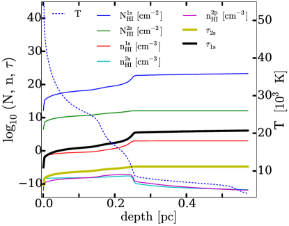
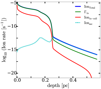
Figure 1.— Several properties of the nebula surrounding the population ${\rm m50M1000a0}$. The parameters used are ${\rm log\,U=-1}$, $\rm n_{H}=10^{3}\,cm^{-3}$ and ${\rm log\,Z/Z_{\odot}=-9}$. The horizontal axis denotes the depth, where the null value is the internal part facing the stellar population. Left panel: The vertical left axis represents the decimal logarithm of the column density, number density and optical depths, with the units shown in the legend. We show the column density (dark blue and green lines) and optical depth (thick lines) for the ground state and first excited state, and the population of the ground state and the two excited states, 2s and 2p, (red and light blue lines) of hydrogen. The vertical right axis denotes the electron temperature (dashed blue line). The region at $r\sim 0.25$ pc denotes the transition from mostly ionized to mostly neutral hydrogen. This happens at a T${}_{e}\sim 10^{4}$ K. Note the low values for the column density and optical depth of the first excited state compared to those for the ground state, which makes the photoionization from the former very unlikely. Note also the high values of the temperature in the ionized region which will be the responsible for collisional excitation of the Ly$\alpha$ line by free electrons. Right panel shows the major contributors to the hydrogen ionization in the nebula. the thin green line denotes the photoionization from the ground state which dominates in the ionized region ($\sim 90\%$ of the total). The collisional ionizations from the ground state (red line) represent $\sim 10\%$ of the total. In the neutral region, the secondary ionizations (dashed blue line) dominate and the photoionization represents $\sim 10-20\%$ of the total.

In this section we first study the existence of departures from the case-B assumption in our populations, shown to be important in metal-free objects by Raiter et al. (2010), and second, we revisit the origin of these departures.

We compute the luminosity for the Ly$\alpha$ and HeII$\,\lambda 1640$ lines assuming case-B recombination, and compare them with the output from Cloudy, always for our lowest metallicity value, ${\rm log\,Z/Z_{\odot}=-9}$, since we expect the differences to be the largest in this case as shown by Raiter et al. (2010). For the same reason, we make use of the populations ${\rm m50M1000a0}$ and ${\rm m9M50a2}$, which present the two most extreme cases of stellar populations.

For the analytical case-B, we follow the assumptions and formalism in Raiter et al. (2010) and we adopt for the nebula an electron density $\rm n_{e}=10^{2}\,cm^{-3}$ and an electron temperature $\rm T_{e}=30\,000\,K$. This implies a conversion of ionizing photons into Ly$\alpha$ of $\sim 68\%$, and yields to the formulae (Schaerer, 2002)

$$L_{\rm\alpha}^{\rm B}=1.04\times 10^{-11}\,{\rm Q(HI)}~{},$$ (2)

$$L_{\rm 1640}^{\rm B}=5.67\times 10^{-12}\,{\rm Q(HeII)}~{},$$ (3)

where ${\rm Q(HI)}$ and ${\rm Q(HeII)}$ are here the photon flux computed by Cloudy for comparative reasons.

The most important results for our further discussion can be summarized as: (i) case-B overestimates the values for the luminosity of the HeII$\,\lambda 1640$ line by a factor $\sim 2$ for the case of high nebular densities, $\rm n_{H}=10^{2}-10^{3}\,cm^{-3}$, and low ionization parameter, ${\rm log\,U=-4}$, for both populations. (ii) The values for the Ly$\alpha$ luminosity are underestimated by a factor $\sim 3$ for our high-mass stars population and $\sim 2$ for the low-mass stars one. These values closely match the mean Lyman continuum photon energy in units of 1 Rydberg (as noted previously by Raiter et al., 2010). For high densities, $\rm n_{H}=10^{2}-10^{3}\,cm^{-3}$, the departures are slightly higher than for lower densities. These results are in very good agreement with those obtained originally by Raiter et al. (2010).

As an explanation for the case-B departure of the Ly$\alpha$ radiation, Raiter et al. (2010) proposed that the high temperatures in the ionized region of the nebula allow for the collisional excitations to populate the first excited state of the hydrogen atom. Then, ionization by low energy photons can occur from that level, thus boosting the emission of Ly$\alpha$ to larger values compared to case-B (which only accounts for photoionizations from the ground state). However, for the photoionization from the first excited state to occur, very large column densities for this state are necessary since the cross section of this transition is of the order $\sigma_{n=2}\sim 10^{-17}\,{\rm cm^{-2}}$. Having a non-negligible optical depth to photoionization from the $n=2$ state may imply that the nebular region becomes optically thick in the HI fine structure lines (see Dijkstra et al., 2016b)

In order to revisit the processes governing the departures from case-B, we use the population ${\rm m50M1000a0}$. The parameters for the nebula are ${\rm log\,U=-1}$, $\rm n_{H}=10^{3}\,cm^{-3}$ and ${\rm log\,Z/Z_{\odot}=-9}$. This set of parameters is the one favouring the largest differences between Cloudy and the analytical calculation. For this population, the mean Lyman continuum photon energy is $2.9$ Ryd.

The left panel in Figure 1 shows several parameters of the nebula as a function of depth (x-axis), where $r$ denotes the distance into the nebula (which begins at $r_{in}=10^{17}\,{\rm cm}$). Two regions besides $\sim 0.25$ pc are clearly visible, denoting the mostly ionized (left part) and mostly neutral (right part) nebular hydrogen regions. The populations for the 2s and 2p excited states (light blue and purple thin lines, respectively) appear to be $\sim 9$ orders of magnitude below that of the ground state (red thin line) in the ionized region, and the difference is larger in the neutral part of the nebula. This difference is the same for the column densities (green and dark blue lines) and similar for the optical depth (yellow and black thick lines), due to differences in the cross-section of the ground and first excited states. This implies that the first excited state is very optically thin to ionizing radiation. The right panel denotes the processes contributing to the hydrogen ionization from Cloudy. In the ionized part, the electron temperature reaches very high values allowing for the collisional processes of ionization from the ground state to be important (red line), representing $\sim 10-15\%$ of the total ionization. The other $\sim 90\%$ is due to photoionization from the ground state (green solid line). In the neutral part, secondary ionizations are the major mechanism (dotted light blue line), although the total ionization rate is now many orders of magnitude lower. In any case, photoionizations from the first excited state are negligible. Cloudy shows that $\sim 40\%$ of the Ly$\alpha$ flux is due to collisionally excited Ly$\alpha$ cooling radiation. Therefore, we conclude that Ly$\alpha$ departures from case-B arise mainly due to collisional excitation and ionization of hydrogen atoms by energetic free electrons. In addition, there is contribution to the Ly$\alpha$ production from the collisional mixing between the 2s and 2p levels for the case of high density regions (Raiter et al., 2010), helium recombinations and secondary ionizations.

3.3. Stochastic IMF effects

We show the effects of the stochastic sampling of the IMF in the two following sections. We first present the results for bursts of star formation at the ZAMS in Section 3.3.1 and then the results regarding time evolution in Section 3.3.2. With this stochasticity study accounting for time evolution we aim to provide a basic framework/intuition for extending our results to more general star formation histories. Our discussion focuses on the default target mass (total stellar mass) 1000 M_⊙, although we also show and discuss the cases with target masses 100 and 10 000 M_⊙.

3.3.1 ZAMS phase

We present the results for the samples containing 10 000 galaxies at the ZAMS, built using the stochastic IMF method described in Section 2.2.1.

Figure 2 shows the normalized distributions of ionizing and LW photon fluxes, relative to the deterministic values (vertical dashed lines), for several IMFs. As expected from previous studies, the stochastic effects are more important for those populations favoring the presence of a low number of massive stars with respect to the total number of stars in a burst, i.e., Salpeter slope, and for high upper mass limit IMFs. The distributions for helium present the broadest shapes ( $>$1 order of magnitude below and a factor  $>$$\sim$3 above the deterministic value for all IMFs except for the flat one). This is due to the strong dependence on the hardness of the spectra, which in turn, depends on the stellar mass distribution in the populations. For the case of hydrogen and LW, the distributions are much narrower since the photon flux in these cases is less sensitive to the stellar mass. The distributions of helium flux for the case of target mass 100 and 10 000 M_⊙ reach a maximum value of $\sim 1$ order of magnitude and less than a factor 2 above the deterministic values, respectively, denoting the sensitivity of the stochastic effects to the target mass. For hydrogen and the LW band, the differences compared to the default target mass are smaller but still significant.

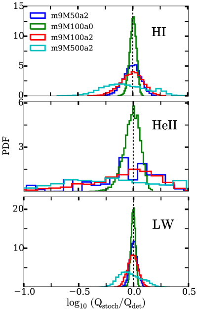
Figure 2.— Normalized distributions of ionizing and LW photon flux for several IMFs relative to the deterministic calculations (vertical dashed line). The target mass value is 1000 M_⊙. From top to bottom, the distributions are for hydrogen, single-ionized helium and LW band. Note the strong stochastic effect for IMFs with Salpeter slopes compared to that for flat IMFs. The HeII distribution shows the broadest shape due to the strong dependence of Q(HeII) on the stellar mass. The stochastic effect increases with higher upper mass limits.

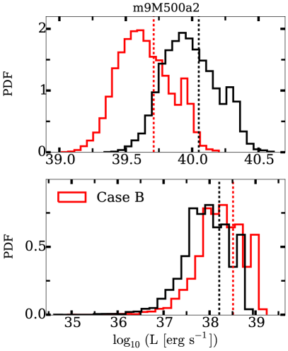
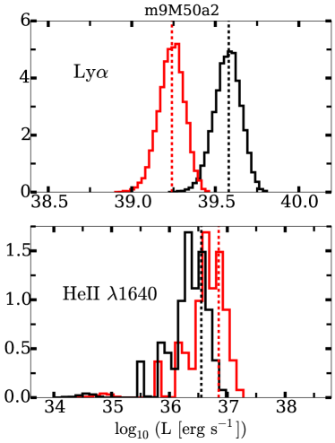
Figure 3.— Upper panels: Normalized Ly$\alpha$ luminosity distributions considering stochastic effects, assuming case-B (red solid lines) and not assuming case-B (black solid lines). Lower panels: Same as before but for HeII$\,\lambda 1640$. Left panels show the cases for the IMF ${\rm m9M500a2}$ and right panels for ${\rm m9M50a2}$. Vertical dashed lines show the deterministic values. The total target mass is 1000 M_⊙. The effect of stochasticity added to the case-B departure can boost the Ly$\alpha$ luminosity a factor $\sim 8$ ($\sim 3.5$) above the common calculations for the case of ${\rm m9M500a2}$ (${\rm m9M50a2}$). The effect of case-B overestimating the HeII$\,\lambda 1640$ luminosity is due to our arbitrary selection of the ionization parameter. For other values of this parameter, the differences between the two distributions are almost null. To facilitate the comparison, the horizontal axis for the same transition in the two IMFs has the same length.

We showed in Section 3.2 that the departure of the Ly$\alpha$ luminosity from the case-B assumption depends on the hardness of the spectra, i.e., on the mean Lyman continuum photon energy. Therefore, stochasticity can further enhance this difference since the hardness of the spectra depends on the distribution of stellar masses. To quantify this effect, we calculate the stochastic distributions for Ly$\alpha$ and HeII$\,\lambda 1640$ luminosities with and without the case-B assumption. We use the IMFs ${\rm m9M500a2}$ and ${\rm m9M50a2}$ as representative for this calculation since they denote the cases where stochasticity has a very high and low effect, respectively. For the case-B calculations we adopt the same formalism as in Section 3.2. Due to the high computational cost of running 10 000 different stellar populations with Cloudy, for the non-case-B calculations we use the fitting formulae given by Raiter et al. (2010) instead. This yields a value for the Ly$\alpha$ luminosity

$$L_{\rm\alpha}=L_{\rm\alpha}^{B}\times\bar{E}\times\frac{\tilde{f}_{\rm coll}}{2/3}~{},$$ (4)

where $L_{\rm\alpha}^{B}$ is the luminosity assuming case-B (Equation 2), $\bar{E}$ denotes the mean Lyman continuum photon energy in Rydbergs and $\tilde{f}_{\rm coll}$ accounts for the density effects. For simplicity, we consider a nebular density $\rm n_{H}=10^{3}\,cm^{-3}$ which yields to $\tilde{f}_{\rm coll}=0.78$ following equation (9) in Raiter et al. (2010). Small variations of the density give rise to a few percent variation in the total result (see section 4.1.1 in Raiter et al., 2010). We assume, again for simplicity, that the ionization parameter is ${\rm log\,U=-4}$. This has no effect on Ly$\alpha$ but implies that case-B overestimates HeII$\,\lambda 1640$ emission by a factor $\sim 2$, due to the actual competition between H and HeII for ionizing photons in cases with low U (Stasińska & Tylenda, 1986; Raiter et al., 2010). We will simply use this value for computing the non case-B helium luminosity. We stress that this is an arbitrary selection and for other values of the ionization parameter and same density, the departures from case-B for the case of helium are almost null (see Figure 10 in Raiter et al., 2010).

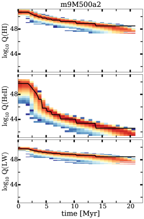
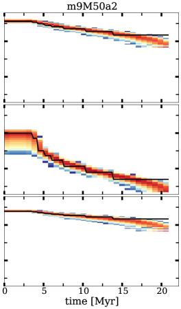
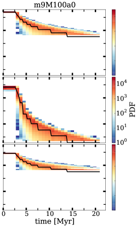
Figure 4.— Normalized distributions of the evolution of photon flux with respect of time for starbursts with IMFs ${\rm m9M500a2}$ (left panel), ${\rm m9M50a2}$ (central panel) and ${\rm m9M100a0}$ (right panel), from left to right, respectively, and for the default target mass 1000 ${\rm M_{\odot}}$. Black solid lines denote the deterministic calculations. For the flat IMF, the distribution broadens rapidly when the first stars start to disappear. To facilitate comparison, all the vertical axis have the same length.

Figure 3 shows the results after these calculations for the default target mass 1000 M_⊙, where the results assuming case-B are plotted in red. The vertical dashed lines show the deterministic values for the corresponding distributions. Left panels present the cases for ${\rm m9M500a2}$ and right panels for ${\rm m9M50a2}$. Upper panels show the results for Ly$\alpha$ and the lower panels those for HeII$\,\lambda 1640$. We see that the HeII$\,\lambda 1640$ luminosity can be boosted by a factor of $~{}\hbox to0.0pt{$>$\hss}{\lower 4.30554pt\hbox{$\sim$}}3$ compared to the deterministic calculation in both populations. The case of Ly$\alpha$ is more interesting since the stochastic boost (a factor $\sim 3$ for ${\rm m9M500a2}$ and $\sim 1.5$ for ${\rm m9M50a2}$) can be added to the departure from case-B (a factor $\sim 2.5$ in both cases). The joint effects may give rise up to a factor $\sim 8$ and $\sim 3.5$ for the respective IMFs compared to the common calculations that do not consider stochasticity and case-B departures. For the 100 M_⊙ target mass, the total Ly$\alpha$ boost can reach a very large value (a factor $\sim 16$ and $\sim 9$ for the two IMFs, respectively) and roughly the same values for the case of helium just accounting for the stochastic effects. The distributions are much narrower for the case of the largest target mass. In this case, the total maximum boosts are hardly above factors of a few in all populations and transitions.

3.3.2 Temporal evolution

In this section, we discuss the results for the distribution of photon fluxes and luminosities taking into account time evolution for two cases: (i) A single burst of star formation, and (ii) allowing for periodic bursts. As before, we use the IMFs ${\rm m9M500a2}$ and ${\rm m9M50a2}$, which have very different sensitivity to stochastic effects, and add now ${\rm m9M100a0}$ to investigate the effect of time to flat IMFs.

First, in Figure 4 we present the evolution of the distribution of photon fluxes considering a single burst of star formation for the default target stellar mass 1000 ${\rm M_{\odot}}$. The black solid lines show the deterministic calculations, which in general follow the peak of the stochastic distributions. The differences at later times exist because the stochastic case can only account for an integer number of stars while the deterministic approximation can take any real number. This can be seen in the last time step of the right panel, where the deterministic number of 9 M_⊙ stars is lower than unity, so the stochastic distribution can never reach those flux values. As expected, the higher upper mass limit IMFs, and specially for the case of helium, present the broadest distributions which, in general for all transitions, tend to slightly broaden with time. This broadening is much more important for the flat IMF, which can reach the minimum value just when the massive stars begin to disappear. This is because in these cases the flat IMF has favored the formation of populations with predominantly massive stars. For the lowest target mass the distributions are much broader and the minimum value of the photon flux can be reached at early times for the same reason as explained above. For the largest target stellar mass the distributions are narrow and show small differences compared to the deterministic calculations.

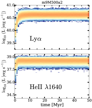
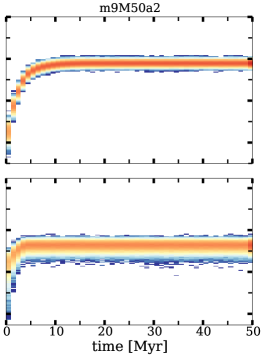
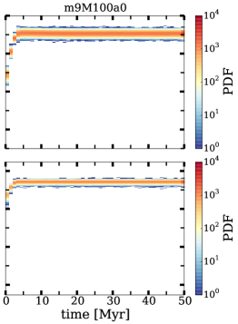
Figure 5.— Normalized distributions for the evolution of luminosities with respect of time, accounting for case-B departures using the formalism shown in Section 3.3.1 and periodic bursts of star formation of 1000 ${\rm M_{\odot}}$ every Myr. From left to right, the IMFs ${\rm m9M500a2}$ (left panel), ${\rm m9M50a2}$ (central panel) and ${\rm m9M100a0}$ (right panel), respectively.

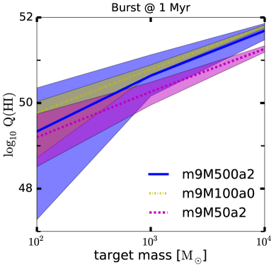
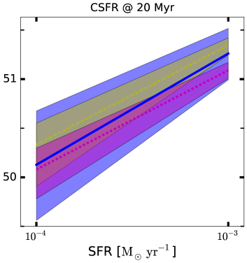
Figure 6.— Evolution of hydrogen photon fluxes for several populations. Left panel shows the case accounting for a single starburst after 1 Myr for our 3 target masses. Lower target masses produce a wider stochastic distribution but cannot compensate for the lower total stellar mass. Right panel shows the case for several bursts after 20 Myr to ensure that the photon flux has reached the flat plateau seen in Figure 5.

Second, we show in Figure 5 the same above distributions but allowing now for periodic bursts of star formation and for the case of Ly$\alpha$ and HeII$\,\lambda 1640$ luminosities. In this case, we create a new stochastic burst using a target mass of 1000 M_⊙ every Myr, which represents an average star formation rate ${\rm SFR}=10^{-3}$ M${}_{\odot}\,{\rm yr^{-1}}$. We account for Ly$\alpha$ departures from case-B adopting the same formalism and values used for Equation 4 in Section 3.3.1 and we assume that there are no departures from case-B for helium. Interestingly, the Ly$\alpha$ luminosity reaches high values, $L_{\rm\alpha}~{}\hbox to0.0pt{$>$\hss}{\lower 4.30554pt\hbox{$\sim$}}5\times 10^{40}\,{\rm erg\,s^{-1}}$, for the populations in the left and right panels, and a factor of $\sim 2-3$ below for the population in the middle panel. For the case of helium, the highest upper mass limit population in the left panel reaches a maximum value of $L_{\rm 1640}\sim 10^{39}\,{\rm erg\,s^{-1}}$ due to the stochastic effects. This plot gives an intuition for the values of the luminosities associated with our models.

Our results can be extrapolated to other target masses and SFRs. Figure 6 shows examples of this for a single starburst after 1 Myr and continuous SFRs after 20 Myr. Note that for the case of a single starburst the values in Figure 6 and the ones for luminosity presented above only last for $2-3$ Myr, while the most massive stars are still alive (Figure 4). Figure 6 shows that when considering a target mass of 100 M_⊙ or ${\rm SFR=10^{-4}}$ M${}_{\odot}\,{\rm yr^{-1}}$, the stochastic effects are larger but not enough to compensate for the reduced total stellar mass. On the other hand, for a target mass of 10 000 M_⊙, the stochastic effects are small but the photon fluxes and luminosities are a factor of $\sim 6-9$ above those for a target mass 1000 M_⊙ due to the larger stellar mass. This implies luminosities as high as $L_{\rm\alpha}\sim 5\times 10^{41}\,{\rm erg\,s^{-1}}$ and $L_{\rm 1640}\sim 6\times 10^{39}\,{\rm erg\,s^{-1}}$. We have checked with a simple linear extrapolation of these fluxes that for higher SFR values the stochastic broadening disappears quickly after SFR$=10^{-3}\,{\rm M_{\odot}\,yr^{-1}}$. Only the stochastic effects for the IMF m9M500a2 are visible slightly further although never reaching the point SFR$=10^{-2}\,{\rm M_{\odot}\,yr^{-1}}$.

In the next section, we discuss the factors that may increase or reduce the luminosity values that we have found and the possibility for a detection of Pop III populations.

4. Discussion

We discuss in this section the factors that can affect our results and the possibility for a detection of Pop III galaxies.

Our stellar populations cover the mass range $9-1000\,{\rm M_{\odot}}$. We adopted the lower mass limit accounting for the validity of the plane parallel assumption in our stellar atmosphere modelling. However, we have tested the inclusion of low mass stars in our stochastic calculations, simply taking the values of photon fluxes for stars down to $1.5\,{\rm M_{\odot}}$ in Marigo et al. (2001). This implies a broadening of the IMFs, i.e., an increase of the stellar mass range. The effect on the stochastic distributions is not very significant for the case of hydrogen photon flux and Ly$\alpha$ luminosities. It is important, however, for the HeII distributions due to their strong dependence on stellar masses. This can reduce the luminosities and photon fluxes of helium by factors $\sim 4-8$, depending on the sensibility to the stochastic effects of the IMF considered.

For simplicity, we have used in our photo-ionization modelling a constant nebular hydrogen density. We note, however, that since we extend our calculations to large time scales, these density values might very well change; e.g., supernova feedback from the most massive stars, stellar winds, changes in the ionizing radiation field, etc. As mentioned before, high nebular densities favor high line luminosities, specially for helium lines, so a decrease of density due to the above processes would be accompanied by a decrease of luminosities at late times. This might be further considered in more detail making use of numerical simulations and radiative transfer codes which can engulf all the necessary physical processes.

We have explored the cases with average star formation rates ${\rm SFR}=10^{-3}$ and ${\rm SFR}=10^{-4}$ M${}_{\odot}\,{\rm yr^{-1}}$. These values are in agreement with the simulations by, e.g., Wise et al. (2012, 2014), but these and other recent studies also allow for lower SFR. Cen (2016) argues that the episodic bursts of star formation in atomic cooling halos are of the order of one every $20-100$ Myr, yielding ${\rm SFR}\sim 10^{-5}$ M${}_{\odot}\,{\rm yr^{-1}}$ or less, depending on the target mass of the bursts. In these cases, the high luminosity and photon flux values that we have obtained would only be present for a few Myr, during the life of the most massive stars.

Pop III stars are usually thought to exist only at very high redshifts, $z>11-25$, but various studies indicate that they can also form at much lower redshifts, up to $z\sim 6-7$ (Scannapieco et al., 2003; Salvadori et al., 2007; Tornatore et al., 2007; Trenti et al., 2009; Wise et al., 2012; Maio et al., 2013; Muratov et al., 2013; Visbal et al., 2016). Recent simulations by Xu et al. (2016) find a non-negligible number of galaxies containing Pop III stars at $z\sim 7$. These stars reside in dark matter halos of masses $M_{h}\sim 10^{7}-10^{8}{\rm M_{\odot}}$ and the total stellar mass covers the range from a few tens to $\sim 1000$ M_⊙, in agreement with our target masses. In some cases, the mean metallicity of the halo is high enough to affect our luminosity results, especially for helium emission lines, but it is also possible that the regions where the stars reside contain only pristine gas (Whalen et al., 2008; Xu et al., 2016). If the metal enrichment by previous stars affects the star forming region, this could also supress the formation of successive metal-free objects, thus reducing the SFR, or even allowing only for an initial burst (Nomoto et al., 2006; Heger & Woosley, 2002).

It is important to mention that the maximum photon flux and luminosities that we have found correspond to the upper tails of the stochastic distributions. When these distributions are broad, specially for m9M500a2, the expected number of stochastic stellar populations giving rise to these values is small and the values in the peaks of the stochastic distributions are far from those in the tails. For this IMF, and considering populations with ages $>10$ Myr in Figure 5, we find that $\sim 0.2\%$ ($\sim 33\%$) of the galaxies have luminosities above $L_{\rm\alpha}=6.5\times 10^{40}$ ($L_{\rm\alpha}=4.5\times 10^{40}$) ${\rm erg\,s^{-1}}$, and $\sim 0.3\%$ ($\sim 22\%$) have values above $L_{\rm 1640}=10^{39}$ ($L_{\rm 1640}=5\times 10^{38}$) ${\rm erg\,s^{-1}}$. The probability for obtaining these extreme values increases and the peaks of the distributions are closer to the tails (the distributions narrow) when considering flatter IMFs. The simple deterministic calculation for m9M500a0 considering Ly$\alpha$ case-B departures and a total stellar mass 1000 M_⊙ (Equation 4) gives luminosities $L_{\rm\alpha}\sim 5\times 10^{40}\,{\rm erg\,s^{-1}}$ and $L_{\rm 1640}\sim 10^{39}\,{\rm erg\,s^{-1}}$, which are similar to those for m9M500a2. The differences between tail and peak values are less important for the other populations with lower upper mass limits.

Many works have investigated the possible detection of Population III galaxies and the use of different techniques to distinguish them from the more ‘normal’ galaxies (see, e.g., Schaerer, 2013, and references therein). This is a difficult task since different factors which are still not fully constrained (e.g., dust, galactic feedback, neutral gas fraction, gravitational lensing, etc.) can contribute to the enhancement or reduction of the intrinsic fluxes during the transmission through the ISM and IGM (e.g., Johnson et al., 2009; Dijkstra et al., 2011; Laursen et al., 2011; Smith et al., 2015). The resonant nature of the Ly$\alpha$ transition adds an extra difficulty in this case, strongly affecting the highly uncertain escape fraction of Ly$\alpha$ photons (e.g., Dijkstra, 2014). We consider the simple case of our default target mass, 1000 M_⊙, with intrinsic luminosity values $L_{\rm\alpha}\sim 5\times 10^{40}\,{\rm erg\,s^{-1}}$ and $L_{\rm 1640}\sim 10^{39}\,{\rm erg\,s^{-1}}$. We calculate the fluxes expected from populations at redshift $z=7,\,10$ and $14$, accounting for the dilution factor due to the luminosity distance, and we compare them with the sensitivity limit of the Near Infrared Spectrograph (NIRSpec) aboard the JWST (Gardner et al., 2006). We consider the case of line fluxes from a point source, with a signal-to-noise, ${\rm SNR}=10$, and $10^{4}$ s of integration time. We find that Ly$\alpha$ luminosity is a factor of $\sim 20$ below the detection threshold at redshifts $z=7$ and $10$, and falls below a factor of $40$ at $z=14$. The helium luminosity is a factor $\sim 450$ below the detection limit at $z=7$ and almost three orders of magnitude below for the highest redshifts. Therefore, higher total stellar masses and/or gravitational lensing (Stark et al., 2007; Zackrisson et al., 2012, 2015) appear to be indispensable for a spectroscopic confirmation of Pop III galaxies (non-metal detection and the presence of strong Ly$\alpha$ emission), and also for detection with, e.g., the combination of wide-field surveys and multiband photometry (see, e.g., Zackrisson et al., 2011a, b; Inoue, 2011).

5. Summary and conclusions

We have revisited the spectra of population III galaxies, specifically focusing on the nebular hydrogen Ly$\alpha$ and ${\rm HeII}\,\lambda 1640$ lines. We have computed a series of stellar helium and hydrogen model atmospheres covering a mass range from ${\rm 9\,to\,1000\,M_{\odot}}$. We have used the stars to construct several populations, allowing for top-heavy and Salpeter slope IMFs, and different upper stellar mass limits. We have included upper mass limits that are lower than those in earlier works, motivated by recent studies favoring the formation of low mass objects, and, for the first time in studies of Pop III populations, we have considered the stochastic sampling of the IMF. We have obtained the nebular spectra using our own SEDs and the photoionization code Cloudy. Finally, we have explored the departures from the case-B recombination assumption for our populations, and we have revisited their origin. Our results can be summarized as follows.

• The Ly$\alpha$ line flux is enhanced by a factor of $2-3$ compared to case-B, depending on the IMF and parameters of the nebula, in agreement with Raiter et al. (2010). Our analysis shows that the origin of the Ly$\alpha$ departures from case-B is due mainly to energetic free electrons which collisionally excite and ionize hydrogen atoms. The photoionization from the first excited state, argued to be the major mechanism in previous works, is negligible.

• Stochastic sampling of the IMF produces large fluctuations in the ionizing photon flux, specially for the single-ionized helium (Q(HeII); more than a factor 100 for a total stellar mass of 1 000 M_⊙), due to the strong dependence on the mass of the stars within the populations. For the case of hydrogen and the LW band, the distributions around the deterministic value are much narrower. The stochastic effects are more important for IMFs with high upper mass limits and also for those which disfavor the presence of massive stars, i.e., those with Salpeter slopes instead of flat IMFs. Stochasticity can enhance the Ly$\alpha$ flux up to a factor $\sim 3$ in populations with massive stars (upper mass limit IMF of 500 M_⊙). This, added to the case-B departure implies a boost by a factor of $\sim 8$ compared to the common calculations. For populations with less massive stars the total boost reaches values $\sim$5, depending on the IMFs and nebular parameters. For the case of the ${\rm HeII}\,\lambda 1640$ line, stochasticity boosts the flux up to a factor $\sim 3$. Accounting for a lower total stellar mass, 100 M_⊙, the stochastic effects increase significantly showing the strong anti-correlation between these two parameters. In this case, the fluctuations found for the hydrogen (LW) ionizing photon fluxes can have implications to the ionizing (dissociating) power inferred for Pop III stars. On the other hand, for a total stellar mass of 10 000 M_⊙, the stochastic effects are strongly reduced.

• When considering the effect of time evolution for a single starburst we see that the distributions slightly broaden with time, specially for the case of flat IMFs. The stochastic effects are again more important for high stellar mass upper limit IMFs and for low values of the total stellar mass. Considering periodic bursts of star formation, we observe similar stochastic behaviours as before, and all the distributions flatten after $~{}\hbox to0.0pt{$<$\hss}{\lower 4.30554pt\hbox{$\sim$}}10$ Myr. The distributions reach maximum intrinsic luminosity values of $L_{\rm\alpha}\sim 5\times 10^{40}\,{\rm erg\,s^{-1}}$ and $L_{\rm 1640}\sim 10^{39}\,{\rm erg\,s^{-1}}$ for a total stellar mass of 1 000 M_⊙. For the case of Ly$\alpha$, these values are a factor $\sim 20$ below the sensitivity limits of the JWST at redshifts $z=7-10$, but this can improve considering the possible effects of gravitational lensing and/or higher total stellar mass. Visbal et al. (2016) have recently presented an analysis which allows for the formation of late ($z\sim 7$), massive ($>10^{6}$ M_⊙) Pop III starbursts in $\sim 10^{9}$ M_⊙ dark matter halos, due to photoionization feedback effects by nearby galaxies. In addition, these stellar populations would likely reside in large ionized bubbles, thus illustrating that the neutral IGM may occasionally have a minor impact on the Ly$\alpha$ flux from Pop III galaxies (see Stark et al., 2016). Stellar populations of such characteristics would be above the detection limits, even for the case of helium fluxes.

We conclude by stressing that the joint effect of the stochastic sampling of the IMF and case-B departures analysed in this work can give rise to values of the Ly$\alpha$ and HeII$\,\lambda 1640$ line fluxes which deviate significantly from the standard analytical calculations which ignore these effects. Our study, as well as previous works, shows that gravitational lensing is required to detect Pop III galaxies with JWST. However, the enhancement obtained in our results reduces significantly the required magnification.

References

- Abel et al. (2002) Abel, T., Bryan, G. L., & Norman, M. L. 2002, Science, 295, 93
- Aoki et al. (2014) Aoki, W., Tominaga, N., Beers, T. C., Honda, S., & Lee, Y. S. 2014, Science, 345, 912
- Bromm (2013) Bromm, V. 2013, Reports on Progress in Physics, 76, 112901
- Bromm et al. (2002) Bromm, V., Coppi, P. S., & Larson, R. B. 2002, ApJ, 564, 23
- Bromm et al. (2001) Bromm, V., Kudritzki, R. P., & Loeb, A. 2001, ApJ, 552, 464
- Bruzual A. (2002) Bruzual A., G. 2002, in IAU Symposium, Vol. 207, Extragalactic Star Clusters, ed. D. P. Geisler, E. K. Grebel, & D. Minniti, 616
- Cen (2016) Cen, R. 2016, ArXiv e-prints [\eprint[arXiv]1604.01986]
- Cerviño & Luridiana (2006) Cerviño, M. & Luridiana, V. 2006, A&A, 451, 475
- Cerviño et al. (2000) Cerviño, M., Luridiana, V., & Castander, F. J. 2000, A&A, 360, L5
- Chen et al. (2016) Chen, K.-J., Heger, A., Whalen, D. J., et al. 2016, ArXiv e-prints [\eprint[arXiv]1601.06896]
- Clark et al. (2011a) Clark, P. C., Glover, S. C. O., Klessen, R. S., & Bromm, V. 2011a, ApJ, 727, 110
- Clark et al. (2011b) Clark, P. C., Glover, S. C. O., Smith, R. J., et al. 2011b, Science, 331, 1040
- da Silva et al. (2012) da Silva, R. L., Fumagalli, M., & Krumholz, M. 2012, ApJ, 745, 145
- da Silva et al. (2014) da Silva, R. L., Fumagalli, M., & Krumholz, M. R. 2014, MNRAS, 444, 3275
- de Bennassuti et al. (2014) de Bennassuti, M., Schneider, R., Valiante, R., & Salvadori, S. 2014, MNRAS, 445, 3039
- Dijkstra (2014) Dijkstra, M. 2014, PASA, 31, 40
- Dijkstra et al. (2016a) Dijkstra, M., Gronke, M., & Sobral, D. 2016a, ArXiv e-prints [\eprint[arXiv]1602.07695]
- Dijkstra et al. (2011) Dijkstra, M., Mesinger, A., & Wyithe, J. S. B. 2011, MNRAS, 414, 2139
- Dijkstra et al. (2016b) Dijkstra, M., Sethi, S., & Loeb, A. 2016b, ApJ, 820, 10
- Ekström et al. (2008) Ekström, S., Meynet, G., Chiappini, C., Hirschi, R., & Maeder, A. 2008, A&A, 489, 685
- Eldridge (2011) Eldridge, J. J. 2011, in Astronomical Society of the Pacific Conference Series, Vol. 440, UP2010: Have Observations Revealed a Variable Upper End of the Initial Mass Function?, ed. M. Treyer, T. Wyder, J. Neill, M. Seibert, & J. Lee, 217
- Erni et al. (2006) Erni, P., Richter, P., Ledoux, C., & Petitjean, P. 2006, A&A, 451, 19
- Ferland et al. (2013) Ferland, G. J., Porter, R. L., van Hoof, P. A. M., et al. 2013, RMXAA, 49, 137
- Forero-Romero & Dijkstra (2013) Forero-Romero, J. E. & Dijkstra, M. 2013, MNRAS, 428, 2163
- Frebel et al. (2009) Frebel, A., Johnson, J. L., & Bromm, V. 2009, MNRAS, 392, L50
- Frebel & Norris (2015) Frebel, A. & Norris, J. E. 2015, ArXiv e-prints [\eprint[arXiv]1501.06921]
- Fumagalli et al. (2011) Fumagalli, M., da Silva, R. L., & Krumholz, M. R. 2011, ApJL, 741, L26
- Gardner et al. (2006) Gardner, J. P., Mather, J. C., Clampin, M., et al. 2006, Space Sci. Rev., 123, 485
- Greif (2015) Greif, T. H. 2015, Computational Astrophysics and Cosmology, 2, 3
- Greif et al. (2011) Greif, T. H., Springel, V., White, S. D. M., et al. 2011, ApJ, 737, 75
- Haas & Anders (2010) Haas, M. R. & Anders, P. 2010, A&A, 512, A79
- Heger & Woosley (2002) Heger, A. & Woosley, S. E. 2002, ApJ, 567, 532
- Hirano et al. (2015) Hirano, S., Hosokawa, T., Yoshida, N., Omukai, K., & Yorke, H. W. 2015, MNRAS, 448, 568
- Hirano et al. (2014) Hirano, S., Hosokawa, T., Yoshida, N., et al. 2014, ApJ, 781, 60
- Hosokawa et al. (2015) Hosokawa, T., Hirano, S., Kuiper, R., et al. 2015, ArXiv e-prints [\eprint[arXiv]1510.01407]
- Hubeny & Lanz (1995) Hubeny, I. & Lanz, T. 1995, ApJ, 439, 875
- Inoue (2010) Inoue, A. K. 2010, MNRAS, 401, 1325
- Inoue (2011) Inoue, A. K. 2011, MNRAS, 415, 2920
- Jimenez & Haiman (2006) Jimenez, R. & Haiman, Z. 2006, Nature, 440, 501
- Johnson et al. (2008) Johnson, J. L., Greif, T. H., & Bromm, V. 2008, in IAU Symposium, Vol. 250, IAU Symposium, ed. F. Bresolin, P. A. Crowther, & J. Puls, 471–482
- Johnson et al. (2009) Johnson, J. L., Greif, T. H., Bromm, V., Klessen, R. S., & Ippolito, J. 2009, MNRAS, 399, 37
- Karlsson et al. (2013) Karlsson, T., Bromm, V., & Bland-Hawthorn, J. 2013, Reviews of Modern Physics, 85, 809
- Karlsson et al. (2008) Karlsson, T., Johnson, J. L., & Bromm, V. 2008, ApJ, 679, 6
- Keller et al. (2014) Keller, S. C., Bessell, M. S., Frebel, A., et al. 2014, Nature, 506, 463
- Krtička & Kubát (2006) Krtička, J. & Kubát, J. 2006, A&A, 446, 1039
- Krtička & Kubát (2009) Krtička, J. & Kubát, J. 2009, A&A, 493, 585
- Krumholz et al. (2015) Krumholz, M. R., Fumagalli, M., da Silva, R. L., Rendahl, T., & Parra, J. 2015, MNRAS, 452, 1447
- Krumholz et al. (2009) Krumholz, M. R., Klein, R. I., McKee, C. F., Offner, S. S. R., & Cunningham, A. J. 2009, Science, 323, 754
- Kubát (2012) Kubát, J. 2012, ApJS, 203, 20
- Kudritzki (2002) Kudritzki, R. P. 2002, ApJ, 577, 389
- Kuiper et al. (2011) Kuiper, R., Klahr, H., Beuther, H., & Henning, T. 2011, ApJ, 732, 20
- Lau et al. (2014) Lau, H. H. B., Izzard, R. G., & Schneider, F. R. N. 2014, A&A, 570, A125
- Laursen et al. (2011) Laursen, P., Sommer-Larsen, J., & Razoumov, A. O. 2011, ApJ, 728, 52
- Lovekin & Guzik (2014) Lovekin, C. C. & Guzik, J. A. 2014, MNRAS, 445, 1766
- Maeder & Meynet (2012) Maeder, A. & Meynet, G. 2012, Reviews of Modern Physics, 84, 25
- Maio et al. (2013) Maio, U., Ciardi, B., & Müller, V. 2013, MNRAS, 435, 1443
- Malhotra & Rhoads (2002) Malhotra, S. & Rhoads, J. E. 2002, ApJL, 565, L71
- Marigo et al. (2003) Marigo, P., Chiosi, C., & Kudritzki, R.-P. 2003, A&A, 399, 617
- Marigo et al. (2001) Marigo, P., Girardi, L., Chiosi, C., & Wood, P. R. 2001, A&A, 371, 152
- McKee & Tan (2008) McKee, C. F. & Tan, J. C. 2008, ApJ, 681, 771
- Muratov et al. (2013) Muratov, A. L., Gnedin, O. Y., Gnedin, N. Y., & Zemp, M. 2013, ApJ, 773, 19
- Nagao et al. (2008) Nagao, T., Sasaki, S. S., Maiolino, R., et al. 2008, ApJ, 680, 100
- Nomoto et al. (2006) Nomoto, K., Tominaga, N., Umeda, H., Kobayashi, C., & Maeda, K. 2006, Nuclear Physics A, 777, 424
- Omukai & Inutsuka (2002) Omukai, K. & Inutsuka, S.-i. 2002, MNRAS, 332, 59
- Osterbrock & Ferland (2006) Osterbrock, D. E. & Ferland, G. J. 2006, Astrophysics of gaseous nebulae and active galactic nuclei
- Pallottini et al. (2015) Pallottini, A., Ferrara, A., Pacucci, F., et al. 2015, MNRAS, 453, 2465
- Pettini et al. (2002) Pettini, M., Ellison, S. L., Bergeron, J., & Petitjean, P. 2002, A&A, 391, 21
- Raiter et al. (2010) Raiter, A., Schaerer, D., & Fosbury, R. A. E. 2010, A&A, 523, A64
- Rauch (2003) Rauch, T. 2003, A&A, 403, 709
- Rydberg et al. (2013) Rydberg, C.-E., Zackrisson, E., Lundqvist, P., & Scott, P. 2013, MNRAS, 429, 3658
- Salvadori et al. (2007) Salvadori, S., Schneider, R., & Ferrara, A. 2007, MNRAS, 381, 647
- Scannapieco et al. (2003) Scannapieco, E., Schneider, R., & Ferrara, A. 2003, ApJ, 589, 35
- Schaerer (2002) Schaerer, D. 2002, A&A, 382, 28
- Schaerer (2003) Schaerer, D. 2003, A&A, 397, 527
- Schaerer (2008) Schaerer, D. 2008, in IAU Symposium, Vol. 255, IAU Symposium, ed. L. K. Hunt, S. C. Madden, & R. Schneider, 66–74
- Schaerer (2013) Schaerer, D. 2013, in Astrophysics and Space Science Library, Vol. 396, Astrophysics and Space Science Library, ed. T. Wiklind, B. Mobasher, & V. Bromm, 345
- Schaerer & Pelló (2002) Schaerer, D. & Pelló, R. 2002, APSS, 281, 475
- Schneider et al. (2002) Schneider, R., Ferrara, A., Natarajan, P., & Omukai, K. 2002, ApJ, 571, 30
- Schneider et al. (2003) Schneider, R., Ferrara, A., Salvaterra, R., Omukai, K., & Bromm, V. 2003, Nature, 422, 869
- Smidt et al. (2016) Smidt, J., Wiggins, B. K., & Johnson, J. L. 2016, ArXiv e-prints [\eprint[arXiv]1603.00888]
- Smith et al. (2016) Smith, A., Bromm, V., & Loeb, A. 2016, ArXiv e-prints [\eprint[arXiv]1602.07639]
- Smith et al. (2015) Smith, A., Safranek-Shrader, C., Bromm, V., & Milosavljević, M. 2015, MNRAS, 449, 4336
- Sobral et al. (2015) Sobral, D., Matthee, J., Darvish, B., et al. 2015, ArXiv e-prints [\eprint[arXiv]1504.01734]
- Stacy & Bromm (2014) Stacy, A. & Bromm, V. 2014, ApJ, 785, 73
- Stacy et al. (2010) Stacy, A., Greif, T. H., & Bromm, V. 2010, MNRAS, 403, 45
- Stacy et al. (2012) Stacy, A., Greif, T. H., & Bromm, V. 2012, MNRAS, 422, 290
- Stark et al. (2016) Stark, D. P., Ellis, R. S., Charlot, S., et al. 2016, ArXiv e-prints [\eprint[arXiv]1606.01304]
- Stark et al. (2007) Stark, D. P., Ellis, R. S., Richard, J., et al. 2007, ApJ, 663, 10
- Stasińska & Tylenda (1986) Stasińska, G. & Tylenda, R. 1986, A&A, 155, 137
- Susa et al. (2014) Susa, H., Hasegawa, K., & Tominaga, N. 2014, ApJ, 792, 32
- Tornatore et al. (2007) Tornatore, L., Ferrara, A., & Schneider, R. 2007, MNRAS, 382, 945
- Trenti et al. (2009) Trenti, M., Stiavelli, M., & Michael Shull, J. 2009, ApJ, 700, 1672
- Tumlinson (2006) Tumlinson, J. 2006, ApJ, 641, 1
- Tumlinson et al. (2001) Tumlinson, J., Giroux, M. L., & Shull, J. M. 2001, ApJL, 550, L1
- Tumlinson & Shull (2000) Tumlinson, J. & Shull, J. M. 2000, ApJL, 528, L65
- Tumlinson et al. (2004) Tumlinson, J., Venkatesan, A., & Shull, J. M. 2004, ApJ, 612, 602
- Turk et al. (2009) Turk, M. J., Abel, T., & O’Shea, B. 2009, Science, 325, 601
- Umeda & Nomoto (2005) Umeda, H. & Nomoto, K. 2005, ApJ, 619, 427
- Vink (2015) Vink, J. S. 2015, in Astrophysics and Space Science Library, Vol. 412, Astrophysics and Space Science Library, ed. J. S. Vink, 77
- Visbal et al. (2016) Visbal, E., Haiman, Z., & Bryan, G. L. 2016, ArXiv e-prints [\eprint[arXiv]1602.04843]
- Whalen et al. (2008) Whalen, D., O’Shea, B. W., Smidt, J., & Norman, M. L. 2008, ApJ, 679, 925
- Wise et al. (2014) Wise, J. H., Demchenko, V. G., Halicek, M. T., et al. 2014, MNRAS, 442, 2560
- Wise et al. (2012) Wise, J. H., Turk, M. J., Norman, M. L., & Abel, T. 2012, ApJ, 745, 50
- Wolfe et al. (2005) Wolfe, A. M., Gawiser, E., & Prochaska, J. X. 2005, ARAA, 43, 861
- Xu et al. (2016) Xu, H., Norman, M. L., O’Shea, B. W., & Wise, J. H. 2016, ArXiv e-prints [\eprint[arXiv]1604.03586]
- Yoon (2014) Yoon, S.-C. 2014, in Multifrequency Behaviour of High Energy Cosmic Sources, 66–70
- Yoon et al. (2012) Yoon, S.-C., Dierks, A., & Langer, N. 2012, A&A, 542, A113
- Zackrisson et al. (2015) Zackrisson, E., González, J., Eriksson, S., et al. 2015, MNRAS, 449, 3057
- Zackrisson et al. (2011a) Zackrisson, E., Inoue, A. K., Rydberg, C.-E., & Duval, F. 2011a, MNRAS, 418, L104
- Zackrisson et al. (2011b) Zackrisson, E., Rydberg, C.-E., Schaerer, D., Östlin, G., & Tuli, M. 2011b, ApJ, 740, 13
- Zackrisson et al. (2012) Zackrisson, E., Zitrin, A., Trenti, M., et al. 2012, MNRAS, 427, 2212