Out-of-equilibrium protocol for Rényi entropies via the Jarzynski equality

Abstract

In recent years entanglement measures, such as the von Neumann and the Rényi entropies, provided a unique opportunity to access elusive feature of quantum many-body systems. However, extracting entanglement properties analytically, experimentally, or in numerical simulations can be a formidable task. Here, by combining the replica trick and the Jarzynski equality we devise a new effective out-of-equilibrium protocol for measuring the equilibrium Rényi entropies. The key idea is to perform a quench in the geometry of the replicas. The Rényi entropies are obtained as the exponential average of the work performed during the quench. We illustrate an application of the method in classical Monte Carlo simulations, although it could be useful in different contexts, such as in quantum Monte Carlo, or experimentally in cold-atom systems. The method is most effective in the quasi-static regime, i.e., for a slow quench. As a benchmark, we compute the Rényi entropies in the Ising universality class in $1$$+$$1$ dimensions. We find perfect agreement with the well-known Conformal Field Theory (CFT) predictions.

I Introduction

In recent years entanglement measures have arisen as new diagnostic tools to unveil universal behaviors in quantum many-body systems. Arguably, the most popular and useful ones are the Rényi entropies and the von Neumann entropy amico-2008 ; calabrese-2009 ; eisert-2010 ; laflorencie-2016 (entanglement entropies). Given a system in a pure state $|\psi\rangle$ and a bipartition into an interval $A$ and its complement (see Figure 1), the Rényi entropies $S_{A}^{{}_{(n)}}$ for part $A$ are defined as

$$S_{A}^{(n)}\equiv-\frac{1}{n-1}\ln\textrm{Tr}\rho_{A}^{n},$$ (1)

with $\rho_{A}\equiv\textrm{Tr}_{B}|\psi\rangle\langle\psi|$ the reduced density matrix of $A$, and $\textrm{Tr}\rho_{A}^{n}$ its $n$-th moment. The limit $n\to 1$ defines the von Nemann entropy $S_{A}\equiv-\textrm{Tr}\rho_{A}\ln\rho_{A}$. Due to $\rho_{A}$ being non-local, extracting $S_{A}^{n()}$ analytically, experimentally, or even in numerical simulations can be a challenging task, execpt for free-fermion and free-boson models, for which the entropies can be obtained exactly in arbitrary dimensions eisler-2009 .

A large class of effective measurement protocols for the Rényi entropies are based on the replica trick. The key observation is that for a generic model $\textrm{Tr}\rho_{A}^{n}$ can be obtained as calabrese-2004

$$\textrm{Tr}\rho_{A}^{n}=\frac{{\mathcal{Z}}_{n}(A)}{{\mathcal{Z}}^{n}}.$$ (2)

where ${\mathcal{Z}}\equiv\textrm{Tr}e^{-\beta{\mathcal{H}}}$, and ${\mathcal{Z}}_{n}(A)$ is the partition function on the so-called $n$-sheets Riemann surface (see Figure 2 (b)), which is defined by “gluing” together $n$ independent replicas of the model through part $A$. Importantly, the replica trick lies at the heart of all the known methods for measuring entanglement in cold-atom experiments cardy-2011 ; abanin-2012 ; daley-2012 ; islam-2015 ; kaufman-2016 ; pichler-2016 . For instance, very recently (see Ref. islam-2015, ) $S_{A}^{{}_{(2)}}$ has been succesfully measured in ultra-cold bosonic systems from the interference between two replicas of a many-body state. Moreover, the ratio of partition functions in (2) can be sampled using classical buividovich-2008 ; caraglio-2008 ; alba-2010 ; gliozzi-2010 ; alba-2011 ; alba-2013 and quantum Monte Carlo techniques hastings-2010 ; melko-2010 ; singh-2011 ; isakov-2011 ; humeniuk-2012 ; kaul-2013 ; inglis-2013 ; iaconis-2013 , providing an efficient method to calculate Rényi entropies. Extensions of these techniques for systems in the continuum herdman-2014 , and interacting fermions zhang-2011 ; tubman-2012 ; mcminis-2013 ; grover-2013 ; assaad-2014 ; broecker-2014 ; wang-2014 ; shao-2015 ; drut-2015 ; drut-2016 ; porter-2016 are also available. Monte Carlo methods work effectively in any dimension and at any temperature, for sign-problem-free models. Oppositely, the Density Matrix Renormalization Group uli-2005 ; uli-2011 (DMRG) provides the most effective way to access the full spectrum of $\rho_{A}$ for one-dimensional systems, whereas is less effective in higher dimensions. A severe issue of all the replica-trick-based protocols is that as the size $\ell$ of $A$ increases, ${\mathcal{Z}}_{n}(A)/{\mathcal{Z}}^{n}$ is dominated by rare configurations. The commonly used strategy to mitigate this issue is based on the increment trick hastings-2010 ; alba-2011 ; humeniuk-2012 . This consists in splitting the ratio in (2) as a product of intermediate terms, which have to be measured separately. Their number typically grows as $\ell$, which is the main drawback of the protocol.

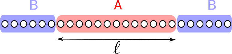
Figure 1: The bipartition used in this work. A chain of length $L$ with periodic boundary conditions is divided into part $A$ of length $\ell$ and its complement $B$. Here we are interested in the Rényi entropy $S^{{}_{(n)}}_{A}$ of $A$.

Here we propose a new out-of-equilibrium framework for measuring the Rényi entropies. Similar protocols to access entanglement in cold-atom experiments have been explored in Ref. cardy-2011, and Ref. abanin-2012, . Our approach combines the replica trick (2) and the Jarzynski equality jarzynski-1997 . Crucially, the latter allows to relate the ratio of partition functions corresponding to two equilibrium thermodynamic states to the exponential average of the work performed during an arbitrary far-from-equilibrium process connecting them. The idea of the method is to modify (i.e., quenching) the geometry of the replicas, gradually driving the system from the geometry with $n$ independent replicas to that of the $n$-sheets Riemann surface. Using the Jarzynski equality, the Rényi entropies are then extracted from the statistics of the work performed during the quench, similar to Ref. cardy-2011, . Some applications of the Jarzyinski equality to detect entanglement have been also presented in Ref. hide-2010, . The efficiency of the method depends dramatically on the rate $\theta$ at which the geometry is modified. Precisely, the number of independent protocol realizations needed increases upon increasing $\theta$. However, in the quasi-static regime, i.e., large $\theta$, $S_{A}^{{}_{(n)}}$ can be extracted from a single realization. In this regime the Rényi entropies depend only on the average work and the standard deviation of the work fluctuations, reflecting that the work distribution function becomes gaussian.

Here we illustrate the approach in the framework of classical Monte Carlo simulations. Specifically, we focus on the Ising universality class in $1$$+$$1$ dimensions, although the method works in any dimension, and it could be extended to quantum Monte Carlo. Remarkably, even for moderately large system sizes the Rényi entropies can be extracted in a single simulation, in contrast with methods using the increment trick, which require typically $\sim\ell$ independent simulations.

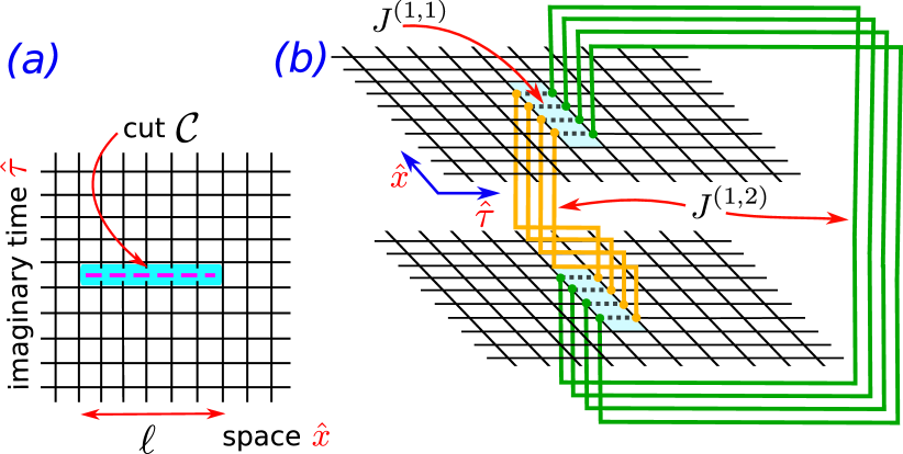
Figure 2: Replica geometry for calculating the Rényi entropy $S^{{}_{(2)}}_{A}$. (a) The single sheet. The vertical and horizontal directions are the imaginary time ($\hat{\tau}$) and spatial ($\hat{x}$) directions, respectively. Periodic boundary conditions in both directions are used. The horizontal dashed line denotes the branch cut ${\mathcal{C}}$ lying on subsystem $A$ (see Figure 2). (b) Two sheets joined through the cut (shaded regions). Spins around the cut and on different replicas interact with coupling $J^{\scriptscriptstyle(1,2)}$. Spins around the cut and on the same replicas interact with couplings $J^{\scriptscriptstyle(1,1)}$ and $J^{\scriptscriptstyle(2,2)}$ (dotted links). The $2$-sheets Riemann surface corresponds to $J^{\scriptscriptstyle(1,1)}=J^{\scriptscriptstyle(2,2)}=0$ and $J^{\scriptscriptstyle(1,2)}=1$. The couplings $J^{{\scriptscriptstyle{(1,2)}}}$ are quenched during the simulation.

II Method: Quenching the replica geometry

The replica geometries used in the method are illustrated in Figure 2. Panel 2 (a) shows a single replica (sheet), where $\hat{x}$ and $\hat{\tau}$ are interpreted as the spatial and imaginary time directions, respectively. The single-sheet partition function ${\mathcal{Z}}$ is obtained as the path integral ${\mathcal{Z}}\equiv\int{\mathcal{D}}[\phi]e^{-{\mathcal{S}}(\{\phi\})}$, where $\phi(x,\tau)$ is a field and ${\mathcal{S}}$ is the euclidean action of the model. We impose the periodic boundary conditions $\phi(x,\tau)=\phi(x,\tau+L_{\tau})$ and $\phi(x,\tau)=\phi(x+L_{x},\tau)$, with $L_{x}$ and $L_{\tau}$ the number of sites along the $\hat{x}$ and $\hat{\tau}$ direction, respectively. For simplicity, we assume interaction only between nearest-neighbor sites $\langle i,j\rangle$, i.e., $S=\sum_{\langle i,j\rangle}F(\phi_{i},\phi_{j})$, with $F$ the interaction strength. In the replica trick (2) one has to consider $n$ replicas of the model ($n$ sheets). The partition function on $n$ independent sheets is ${\mathcal{Z}}^{n}=\int\prod_{k=1}^{n}{\mathcal{D}}[\phi^{{}_{(k)}}]e^{-\sum_{k}{\mathcal{S}}(\{\phi^{{}_{(k)}}\})}$, where $\phi^{{}_{(k)}}$ now denote fields living on the replica $k$. We now consider the situation with $n$ coupled sheets. First, on each sheet a branch cut ${\mathcal{C}}$ lying along the spatial direction is introduced (as in Figure 2 (a)). The $n$ replicas are coupled through ${\mathcal{C}}$ (for $n=2$ see Figure 2 (b)). The partition function on the $n$ coupled sheets is $\widetilde{\mathcal{Z}}_{n}(A)=\int\prod_{k}{\mathcal{D}}[\phi^{{}_{(k)}}]e^{-{\mathcal{S}}^{(n)}(\{\phi^{{}_{(k)}}\})}$, where

$${\mathcal{S}}^{(n)}=\sum\limits_{k=1}^{n}\Big{\{}\sum\limits_{\langle i,j\rangle\not\perp{\mathcal{C}}}F(\phi^{{}_{(k)}}_{i},\phi^{{}_{(k)}}_{j})\\ +\sum\limits_{\!\!\!\!\langle i,j\rangle\perp{\mathcal{C}}}\Big{[}J^{(k,k)}F(\phi^{{}_{(k)}}_{i},\phi^{{}_{(k)}}_{j})+J^{(k,k+1)}F(\phi^{{}_{(k)}}_{i},\phi^{{}_{(k+1)}}_{j})\Big{]}\Big{\}}.$$ (3)

Here $\langle i,j\rangle\perp{\mathcal{C}}$ denotes links crossing the cut, and $J^{\scriptscriptstyle(k,k^{\prime})}$ is the coupling between fields next to cut and living on replicas $k$ and $k^{\prime}$. The replicas are coupled in a cyclic fashion, meaning that the replica indices $k,k^{\prime}$ are defined $\textrm{mod}\,n$. The partition function on the $n$-sheets Riemann surface ${\mathcal{Z}}_{n}(A)$ (cf. (2)) corresponds to $J^{\scriptscriptstyle(k,k^{\prime})}=\delta_{k^{\prime},k+1}$.

Any ratio $\widetilde{\mathcal{Z}}_{n}/{\mathcal{Z}}^{n}$ can be calculated using the Jarzynski equality jarzynski-1997 . Specifically, let us consider a system at equilibrium at an initial time $t_{i}$. Let ${\mathcal{Z}}_{i}$ be its partition function. Now let us imagine that the system is driven to a new equilibrium state at $t_{f}$, which is described by ${\mathcal{Z}}_{f}$, using an arbitrary out-of-equilibrium protocol. For an Hamiltonian system this could be a quench, in which some parameters of the Hamiltonian ${\mathcal{H}}(t)$ are varied with time. The Jarzynski equality states that

$$\Big{\langle}\exp\Big{[}-\beta\int_{t_{i}}^{t_{f}}dt\delta W(t)\Big{]}\Big{\rangle}=\frac{{\mathcal{Z}}_{f}}{{\mathcal{Z}}_{i}}.$$ (4)

Here $\delta W\equiv{\mathcal{H}}(t+dt)-{\mathcal{H}}(t)$ is the infinitesimal work performed between time $t$ and $t+dt$, $\beta\equiv 1/T$ is the inverse temperature, and $\langle\cdot\rangle$ denotes the average over different realizations of the quench protocol. The Jarzynski equality has been verified in several systems, and it is routinely used to extract free energy differences in out-of-equilibrium experiments hummer-2001 ; liphardt-2002 ; douarche-2005 ; collin-2005 ; bustamante-2005 ; blickle-2006 ; harris-2007 ; saira-2012 ; jarzynski-2011 ; seifert-2012 ; shuoming-2015 , and in Monte Carlo simulations (see for instance Ref. caselle-2016 ).

The idea of our method is to use (4) performing a quench of the couplings $J^{\scriptscriptstyle(k,k^{\prime})}$ (cf. (3)) from the starting configuration with $J^{\scriptscriptstyle(k,k^{\prime})}=\delta_{k,k^{\prime}}$ ($n$ independent replicas) and final one with $J^{\scriptscriptstyle(k,k^{\prime})}=\delta_{k^{\prime},k+1}$ (coupled replicas). Any quench protocol is expected to give the same result. We choose the ramp protocol

$$J^{(k,k^{\prime})}=\left\{\begin{array}[]{cc}\delta_{k,k^{\prime}}&\textrm{if}\,\,t\leq t_{i}\\ \frac{t-t_{i}}{t_{f}-t_{i}}(\delta_{k^{\prime},k+1}-\delta_{k,k^{\prime}})+\delta_{k,k^{\prime}}&\textrm{if}\,\,t>t_{i}\end{array}\right.$$ (5)

Here $t$ is the Monte Carlo time, and $1/(t_{f}-t_{i})\equiv\theta$ is the quenching rate. Importantly, $t_{i}$ has to be large enough to ensure initial thermal equilibrium.

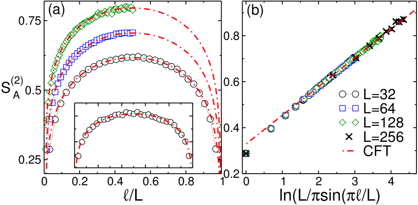
Figure 3: Rényi entropy $S^{{}_{(2)}}_{A}$ in the Ising universality class in $1$$+$$1$ dimensions: Numerical results using the out-of-equilibrium Monte Carlo method. Panel (a): $S^{{}_{(2)}}_{A}$ plotted as a function of $\ell/L$, with $\ell$ the length of $A$ and $L=L_{x}$ (see Figure 2). Note for $L=32$ the expected symmetry under $\ell\to L-\ell$. The dashed-dotted lines are one-parameter fits to the CFT prediction $S_{A}^{{}_{(2)}}=c/3\log(L/\pi\sin(\pi\ell/L))+k$, with $c=1/2$ the central charge and $k$ a constant. Inset: $S^{{}_{(2)}}_{A}$ as obtained from a single simulation. The dashed-dotted line is the same as in the main Figure. Panel (b): Same data as in (a) plotted versus $\log(L/\pi\sin(\pi\ell/L))$. The straight lines are the same as in (a).

Using (2) and (4), the Rényi entropy is obtained as

$$S_{A}^{(n)}=\frac{1}{n-1}\ln\big{[}\langle\exp(-\beta W)\rangle\big{]},$$ (6)

where $W$ is the integrated work performed during the Monte Carlo history, i.e., $W=(t_{f}-t_{i})^{-1}\sum_{t=t_{i}}^{t_{f}}\delta{\mathcal{S}}^{(n)}(t)$, and $\delta{\mathcal{S}}^{(n)}$ is the change in energy between two consecutive Monte Carlo steps $t_{i}$ and $t_{i+1}$, calculated using the field configurations at $t_{i}$, i.e.,

$$\delta{\mathcal{S}}^{(n)}=\sum\limits_{k,\langle i,j\rangle\perp{\mathcal{C}}}[F(\phi^{{}_{(k)}}_{i},\phi^{{}_{(k+1)}}_{j})-F(\phi^{{}_{(k)}}_{i},\phi^{{}_{(k)}}_{j})].$$ (7)

Importantly, Eq. (6) implies that $S_{A}^{{}_{(n)}}$ depends on the full work distribution function (similar to Ref. cardy-2011, ). Remarkably, in the quasi-static regime one has

$$S^{(n)}_{A}=\frac{\beta}{n-1}\Big{[}-\langle W\rangle+\beta\frac{\sigma_{W}^{2}}{2}\Big{]},$$ (8)

where $\sigma_{W}^{2}\equiv\langle W^{2}\rangle-\langle W\rangle^{2}$ is the work variance. Eq. (8) is derived assuming that the work distribution function is gaussian, and it is also known as Callen-Welton fluctuation dissipation relation callen-1951 . The second term in (8) corresponds to the work $W_{d}$ dissipated during the quench. Interestingly, Eq. (6) implies that the number of independent simulations needed to obtain a reasonable estimate of $S_{A}^{{}_{(n)}}$ increases exponentially with $W_{d}$ (see Ref. jarzynski-2006, for a rigorous result). On the other hand from (8), one has that $\sigma_{W}\to 0$ in the quasi-static limit $\theta\to\infty$, implying that $S_{A}^{{}_{(n)}}$ can be extracted from a single protocol realization.

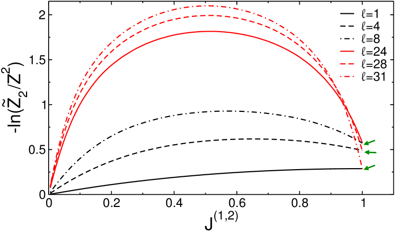
Figure 4: Monte Carlo dynamics of the entropy estimator $-\ln({\mathcal{Z}}_{2}/{\mathcal{Z}}^{2})$. Here $-\ln({\mathcal{Z}}_{2}/{\mathcal{Z}}^{2})$ is plotted versus the inter-replicas coupling $J^{\scriptscriptstyle(1,2)}$. Different lines correspond to different sizes $\ell$ of $A$. Data are for a chain with $L=32$ sites, averaged over $\sim 10$ realizations of the quench. Note the maximum a $J^{\scriptscriptstyle(1,2)}\approx 1/2$. Note also at $J^{\scriptscriptstyle(1,2)}=1$ the expected symmetry under the exchange $\ell\to L-\ell$.

III Numerical checks in the Ising universality class

We now provide numerical evidence supporting the correctness and efficiency of our Monte Carlo method. We consider the two-dimensional classical critical Ising model (cf. (10)). The model has a critical point at $\beta_{c}=\ln(1+\sqrt{2})/2$. Here we consider very elongated lattices with $L_{\tau}/L_{x}\gg 1$ (anisotropic limit). In this limit universal properties are the same as in the one-dimensional quantum critical Ising chain at zero temperature, which is defined by the Hamiltonian ${\mathcal{H}}=-\sum_{i=1}^{L_{x}}(\sigma_{i}^{x}\sigma_{i+1}^{x}+\sigma_{i}^{z})$, with $\sigma^{x,z}_{i}$ the Pauli matrices acting on site $i$ of the chain. The critical behavior of both models is described by a Conformal Field Theory yellow-book (CFT) with central charge $c=1/2$.

In our Monte Carlo simulations we employed the Swendsen-Wang method swendsen-1987 , although any other type of update can be used. In the Swendsen-Wang update, at any Monte Carlo time $t$ one assigns to each link of the lattice (here the connected $n$ replicas, see Figure 2 (b)) an auxiliary activation variable. Links connecting pairs of aligned spins and not crossing the branch cut are then activated with probability $p=1-\exp(-2\beta)$, while links connecting aligned spins around the branch cut are activated with probability $p^{\prime}=1-\exp(-2\beta J^{\scriptscriptstyle(k,k^{\prime})})$, with $J^{\scriptscriptstyle(k,k^{\prime})}$ given in (5). In our Monte Carlo simulations we fixed $t_{i}\approx 10^{5}$ and $t_{f}\approx 10^{6}$. Then, all the different clusters of spins are identified using the rule that pairs of spins connected by an activated link are in the same cluster. Finally, all the spins belonging to the same cluster are flipped with probability $p=1/2$.

We should mention that for models that can be mapped to the random cluster model, à la Fortuin Kasteleyn, it is usually convenient to write Monte Carlo observables in terms of cluster-related variables. Typically, at least for equilibrium simulations, this leads to a considerable speedup. This can be done for the Rényi entropy estimator (6), as we discuss in A. Surprisingly, our results suggest that the cluster estimator performs worse than the standard local estimator (6). This is in contrast with cluster estimators for the Rényi entropies in equilibrium Monte Carlo simulations, which outperform local estimators caraglio-2008 .

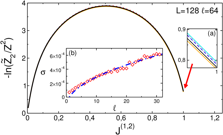
Figure 5: Convergence of the out-of-equilibrium Monte Carlo method for calculating the Rényi entropies. $-\ln(\widetilde{\mathcal{Z}}_{2}/{\mathcal{Z}}^{2})$ plotted as a function of the inter-replicas coupling $J^{\scriptscriptstyle(1,2)}$. Here $J^{\scriptscriptstyle(1,2)}$ is varied during the Monte Carlo dynamics using (5). The different lines correspond to different realizations of the out-of-equilibrium dynamics. Inset (a): Fluctuations of $-\ln(\widetilde{\mathcal{Z}}_{2}/{\mathcal{Z}}^{2})$ around $J^{\scriptscriptstyle(1,2)}=1$. Inset (b): Standard deviation $\sigma$ of the fluctuations of $-\ln(\widetilde{\mathcal{Z}}_{2}/{\mathcal{Z}}^{2})$ at $J^{\scriptscriptstyle(1,2)}=1$ plotted versus the subsystem length $\ell$. The data are for a chain with $L=32$ sites. The standard deviation is calculated using $\sim 250$ independent realizations of the out-of-equilibrium protocol. The dashed-dotted line is a fit to the behavior $\propto\ell^{1/2}$.

The results for $S_{A}^{{}_{(2)}}$ are illustrated in Figure 3. Panel (a) shows $S^{{}_{(2)}}_{A}$ as obtained using (6) and plotted versus $\ell/L$. The symbols are Monte Carlo data for system sizes with $L=32,64,128$, averaged over $\sim 10$ independent realizations of the driving protocol. In the scaling limit $\ell,L\to\infty$, the behavior of $S_{A}^{{}_{(n)}}$ is obtained from CFT as calabrese-2004

$$S_{A}^{(n)}=\frac{c}{6}\Big{(}1+\frac{1}{n}\Big{)}\ln\Big{[}\frac{L}{\pi}\sin\Big{(}\frac{\pi\ell}{L}\Big{)}\Big{]}+k_{n},$$ (9)

where $c=1/2$ is the central charge and $k_{n}$ a non universal constant. The dashed-dotted lines in the Figure are obtained from (9) by fitting $k_{n}$, after fixing $c=1/2$. The good agreement with the data confirms the validity of the method. This is also clear from the perfect linear behavior in panel (b), where we plot $S_{A}^{{}_{(2)}}$ versus $\ln[L/\pi\sin(\pi\ell/L)]$. The inset in Figure 3 (a) plots $S_{A}^{{}_{2}}$ as obtained from a single realization of the driving protocol, i.e., a single Monte Carlo simulation. The dashed-dotted line is the same as in the main Figure. The good agreement with the data suggests that the protocol (5) with $t_{f}\approx 10^{6}$ is already close to the quasi-static regime, at least for $L=32$.

It is also interesting to investigate the behavior of $-\ln(\widetilde{\mathcal{Z}}_{2}/{\mathcal{Z}}^{2})$ as a function of the value of $J^{\scriptscriptstyle(1,2)}$ during the Monte Carlo dynamics. This is discussed in Figure 4. The data are for a single realization of the driving protocol. At $J^{\scriptscriptstyle(1,2)}\approx 0$, one has $-\log(\widetilde{\mathcal{Z}}_{2}/{\mathcal{Z}}^{2})\approx 0$, reflecting that at the early stage of the Monte Carlo the two replicas are disconnected. Interestingly, $-\log(\widetilde{\mathcal{Z}}_{2}/{\mathcal{Z}}^{2})$ exhibits a maximum around $J^{\scriptscriptstyle(1,2)}\approx 1/2$. The expected symmetry $S^{{}_{(2)}}_{A}(\ell)=S_{A}^{{}_{(2)}}(L-\ell)$, which reflects that the zero-temperature one-dimensional system is in a pure state, is observed only at $J^{\scriptscriptstyle(1,2)}=1$ (see arrows in the Figure).

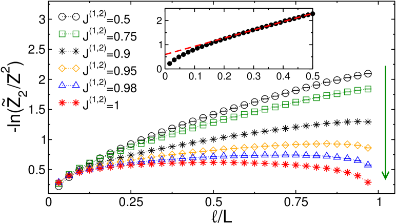
Figure 6: Monte Carlo evolution of the Rényi entropy estimator $-\ln(\widetilde{\mathcal{Z}}_{2}/{\mathcal{Z}}^{2})$. Here $-\ln(\widetilde{\mathcal{Z}}_{2}/{\mathcal{Z}}^{2})$ is plotted against $\ell/L$, with $\ell$ and $L$ the subsystem the chain size, respectively. Different symbols correspond to different values of $J^{\scriptscriptstyle(1,2)}$. The data are for $L=32$. Inset: The same as in the main figure for $L=64$ at $J^{\scriptstyle(1,2)}=1/2$. The dashed line is a linear fit.

We now discuss the fluctuations of $S_{A}^{{}_{(2)}}$ between different realizations of the driving protocol. Figure 5 plots $-\log(\widetilde{\mathcal{Z}}_{2}/{\mathcal{Z}}^{2})$ as a function of $J^{\scriptscriptstyle(1,2)}$ for $10$ independent realizations of the driving protocol. The inset (a) shows a zoom around the region $J^{\scriptscriptstyle(1,2)}\approx 1$. Fluctuations between different realizations of the dynamics are of the order of a few percents. The behavior as a function of $\ell$ of the statistical error $\sigma$ associated with the fluctuations between different realizations is illustrated in inset (b). Here $\sigma$ is calculated as the standard deviation of the fluctuations, considering a sample of $\sim 250$ independent simulations. Clearly, $\sigma$ increases mildly as a function of $\ell$. The dashed-dotted line in the inset is a fit to $\propto\ell^{1/2}$. Finally, it is interesting to investigate the dependence of $-\log(\widetilde{\mathcal{Z}}_{2}/{\mathcal{Z}}^{2})$ on $J^{\scriptscriptstyle(1,2)}$. Figure 6 shows $-\log(\widetilde{\mathcal{Z}}_{2}/{\mathcal{Z}}^{2})$ as a function of $\ell/L$ for several values of $J^{\scriptscriptstyle(1,2)}$. Most notably, for any $J^{\scriptscriptstyle(1,2)}<1$ one has that the symmetry $S_{A}^{{}_{(2)}}(\ell)=S_{A}^{{}_{(2)}}(L-\ell)$ is not present. We should mention that this resembles the behavior of $S_{A}^{{}_{(n)}}$ when the total system is not pure, for instance at finite temperature. Moreover, the data for $J\neq 1$ suggest a volume-law behavior $S_{A}^{(2)}\propto\ell$ (see inset in Figure 6), again as in finite temperature systems.

IV Conclusions

We presented a novel out-of-equilibrium framework for measuring the Rényi entropies by combining the Jarzynski equality and the replica-trick. As an application, we presented a new classical Monte Carlo method to measure the Rényi entropies.

This work opens numerous research directions. First, it would be useful to implement the approach in the framework of quantum Monte Carlo. Furthermore, it would interesting to understand analytically the behavior of $-\log({\mathcal{Z}}_{2}/{\mathcal{Z}}^{2})$ as a function of $J^{\scriptscriptstyle(1,2)}$ (see Figure 6). An intriguing possibility is that $J^{\scriptscriptstyle(1,2)}$ could be interpreted as a finite-temperature for the one-dimensional system. This could provide an alternative way to obtain the finite-temperature Rényi entropies. Interestingly, our approach could be used for the moments of the partially transposed reduced density matrix alba-2013 ; chung-2014 . These are the main ingredients to construct the logarithmic negativity vidal-2002 ; plenio-2005 ; calabrese-2012 , which is a good entanglement measure for mixed states. Another interesting direction is to consider a protocol in which the length of $A$ is also quenched. This would allow to obtain the entropies for different subsystem sizes in a single simulation. Finally, it is important to understand whether our framework could provide a viable alternative to measure Rényi entropies in cold-atom experiments or in NMR quantum simulators fan-2016 ; li-2016 .

Acknowledgments.—

I am greatly indebted with Claudio Bonati for drawing to my attention Ref. caselle-2016, and for useful discussions. I thank Pasquale Calabrese and Paola Ruggiero for reading the manuscript and for useful suggestions. I acknowledge support from the ERC under the Starting Grant 279391 EDEQS. This project has received funding fromt the European Union’s Horizon 2020 research and innovation programme under the Marie Sklodowoska-Curie grant agreement No 702612.

Appendix A Cluster estimator for the Rényi entropies

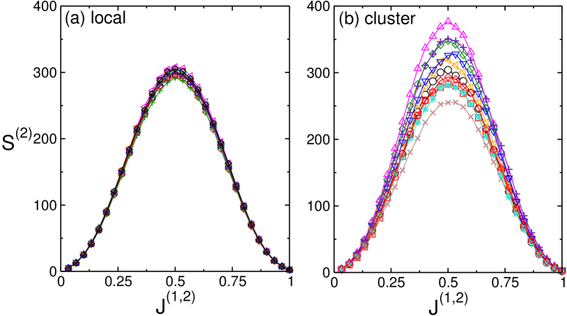
Figure 7: Comparison between the standard estimator for the Rényi entropy $S^{(2)}$ (panel (a)) and the cluster-based one (panel (b)). In both panels $S^{(2)}$ is plotted versus the inter-replica coupling $J^{\scriptscriptstyle(1,2)}$. The different symbols correspond to different realizations of the out-of-equilibrium protocol. The data are for a system with $L_{y}=256$ and subsystem size $\ell=101$. Note that the cluster estimator exhibits larger fluctuations between different realizations of the protocol.

For statistical models that are mappable to the random cluster model, i.e., whose partition function admits a representation á la Fortuin Kasteleyn fk-1969 , it is possible to rewrite (7) in terms of cluster variables (see Ref. caraglio-2008, and alba-2013, for similar results in equilibrium Monte Carlo simulations). Typically, this leads to improved estimators with much smaller variance, as compared with the standard one expressed in terms of spin variables. The physical reason is that each fixed cluster configuration corresponds to many spin configurations. To be concrete, we focus on the two-dimensional Ising model on a square lattice, which is defined by the Hamiltonian

$$H=-J\sum\limits_{\langle i,j\rangle}S_{i}S_{j},$$ (10)

where $S_{i}=\pm 1$ and $J$ is the coupling strength. The partition function of the Ising model at inverse temperature $\beta$ can be expressed using the Fortuin Kasteleyn representation as

$${\mathcal{Z}}=\sum\limits_{\gamma\in\Omega}\Big{\{}\prod\limits_{e\in E}p^{\omega(e)}(1-p)^{1-\omega(e)}\Big{\}}2^{\kappa(\gamma)}.$$ (11)

Here the sum is over the set of subgraphs $\gamma$ on the lattice, i.e., arbitrary sets of lattice sites, $\omega(e)=1$ denotes the (activated) links connecting points in $\gamma$ (it is $\omega=0$ for the other links), while $\kappa(\gamma)$ is the number of connected components of $\gamma$ (clusters). In (11), we defined $p=1-e^{-2\beta J}$.

To calculate $\textrm{Tr}\rho_{A}^{n}$, one first considers a stack of $n$ disconnected replicas of the model and of (11). Each configuration of activated links (cluster configuration) on the disconnected sheets is also a valid one on the $n$-sheets Riemann surface (see Figure 2), in which the copies are connected. The only difference is that now activated links across the branch cut connect sites on different replicas. Importantly, the same configuration of activated links corresponds to different numbers of clusters on the $n$ independent sheets and the Riemann surface. The ratio of partition functions in (2) is written as

$$\textrm{Tr}\rho_{A}^{n}=\frac{{\mathcal{Z}}_{n}(A)}{{\mathcal{Z}}^{n}}=\langle 2^{\kappa_{\mathcal{C}}-\kappa}\rangle_{n},$$ (12)

where, given a fixed set of activated links, $\kappa_{\mathcal{C}}$ is the total number of clusters on the $n$-sheets Riemann surface with cut ${\mathcal{C}}$, while $\kappa$ is the total number of clusters for the model on the $n$ independent sheets. In (12) the statistical average $\langle\cdot\rangle_{n}$ is performed using the model defined on the $n$ independent sheets. Interestingly, from formula (12) one has that the entropies depend only on the number of clusters.

In our out-of-equilibrium setup the Monte Carlo dynamics happens on the coupled $n$ sheets (see Figure 2). Clearly, the Fortuin-Kasteleyn representation (11) still holds. However, in contrast to (11), the probability $p$ of activating the links across the branch cuts are dynamical variables (cf. (5)). On the other hand, since the change in energy $\delta{\mathcal{S}}^{(n)}$ (cf. (7)) is calculated at fixed fields configuration, the number of clusters does not change between two consecutive Monte Carlo updates. Thus, one has

$$S_{A}^{(n)}=\frac{1}{n-1}\ln\Big{[}\Big{\langle}\exp\Big{(}-\sum_{t=t_{i}}^{t_{f}}\delta W_{c}(t)\Big{)}\Big{\rangle}\Big{]},$$ (13)

with

$$\delta W_{c}(t)\equiv\sum\limits_{e\perp{\mathcal{C}}}\ln\Big{(}\frac{p(t+\delta t)}{p(t)}\Big{)}^{\omega(e)}\Big{(}\frac{1-p(t+\delta t)}{1-p(t)}\Big{)}^{1-\omega(e)}.$$ (14)

In the definition of $\delta W_{c}$ the product is over all the links across the branch cut, which connect sites both on the same sheet and on different ones, $p(t)=1-\exp(-2\beta J^{{}_{(k,k^{\prime})}})$, with $J^{{}_{(k,k^{\prime})}}$ as defined in (5), and $\delta t=1/(t_{f}-t_{i})$. For small $\delta t$, which is always the case in the simulations, from (14) one obtains

$$\delta W_{c}(t)=\sum\limits_{e\perp{\mathcal{C}}}\frac{(\omega(e)-p)\delta p}{(1-p)p},$$ (15)

where $\delta p\equiv p(t+\delta t)-p(t)$. It is interesting to observe that (13) does not depend explicitly on the number of clusters, in contrast to (12).

The strategy to use (14) and (13) in Monte Carlo simulations is straightforward using the Swendsen-Wang algorithm. Between two successive update steps of the Monte Carlo one has to measure both $p(t)$ and $p(t+\delta t)$, which are then substituted in (14). Note that in (14), the sum is over the links crossing the branch cuts, and $\omega(e)=1$ only if the link $e$ is active. Thus, the infinitesimal work $\delta W_{c}$ obtained from (14) is integrated on the Monte Carlo history, to obtain the exponent in (13).

The validity and efficiency of (14) is investigated in Figure 7. Panels (a) and (b) show the Rényi entropy $S^{(2)}$ calculated using (6) and (14), respectively. The data are for the critical Ising model on the lattice with $L_{y}=256$ and $L_{x}=2560$, and for a subystem with $\ell=101$ sites. In the Figure, $S^{(2)}$ is plotted versus the inter-replica coupling $J^{\scriptscriptstyle(1,2)}$. In both panels the data are obtained from simulations with $\sim 150000$ Monte Carlo steps. The different symbols correspond to different realization of the out-of-equilibrium protocol. Surprisingly, the data obtained using the cluter estimator (14) (panel(b)) show much larger fluctuations between different realizations as compared with the local estimator (6) (panel (a)). This is in costrast with equilibrium Monte Carlo simulations for calculating the Rényi entropies, where cluster estimators performs better than local ones caraglio-2008

References

- (1) L. Amico, R. Fazio, A. Osterloh, and V. Vedral, Rev. Mod. Phys. 80, 517 (2008).
- (2) P. Calabrese, J. Cardy, and B. Doyon Eds, J. Phys. A 42, 500301 (2009).
- (3) J. Eisert, M. Cramer, and M. B. Plenio, Rev. Mod. Phys. 82, 277 (2010).
- (4) N. Laflorencie, arXiv:1512.03388.
- (5) V. Eisler and I. Peschel, J. Phys. A: Math. Theor. 42 504003 (2009).
- (6) P. Calabrese and J. Cardy, J. Stat. Mech.: Theor. Exp. P06002 (2004).
- (7) J. Cardy, Phys. Rev. Lett. 106, 150404 (2011).
- (8) D. A. Abanin and E. Demler, Phys. Rev. Lett. 109, 020504 (2012).
- (9) A. J. Daley, H. Pichler, J. Schachenmayer, and P. Zoller, Phys. Rev. Lett. 109, 020505 (2012).
- (10) R. Islam, R. Ma, P. M. Preiss, M. E. Tai, A. Lukin, M. Rispoli, and M. Greiner, Nature 528, 77 (2015).
- (11) A. M. Kaufman, M. E. Tai, A. Lukin, M. Rispoli, R. Schittko, P. M. Preiss, and M. Greiner, arXiv:1603.04409
- (12) H. Pichler, G. Zhu, A. Seif, P. Zoller, and M. Hafezi, arXiv:1605.08624.
- (13) P. V. Buividovich and M. I. Polikarpov, Nucl. Phys. B 802, 458 (2008).
- (14) M. Caraglio and F. Gliozzi, JHEP 11, 076 (2008).
- (15) V. Alba, L. Tagliacozzo, and P. Calabrese, Phys. Rev. B 81, 060411 (2010).
- (16) F. Gliozzi and L. Tagliacozzo, J. Stat. Mech.: Theor. Exp., P01002 (2010).
- (17) V. Alba, L. Tagliacozzo, and P. Calabrese, J. Stat. Mech.: Theor. Exp. ,P06012 (2011).
- (18) V. Alba, J. Stat. Mech.: Theor. Exp. P05013 (2013).
- (19) M. B. Hastings, I. Gonzalez, A. B. Kallin, and R. G. Melko, Phys. Rev. Lett. 104, 157201 (2010).
- (20) R. G. Melko, A. B. Kallin, and M. B. Hastings, Phys. Rev. B 82, 100409 (2010).
- (21) R. R. P. Singh, M. B. Hastings, A. B. Kallin, and R. G. Melko, Phys. Rev. Lett. 106, 135701 (2011).
- (22) S. V. Isakov, M. B. Hastings, and R. G. Melko, Nature Physics 7, 772 (2011).
- (23) S. Humeniuk and T. Roscilde, Phys. Rev. B 86, 235116 (2012).
- (24) R. K. Kaul, R. G. Melko, and A. W. Sandvik, Ann. Rev. Cond. Matt. Phys. 4, 179 (2013).
- (25) S. Inglis and R. G. Melko, Phys. Rev. E 87, 013306 (2013).
- (26) J. Iaconis, S. Inglis, A. B. Kallin, and R. G. Melko, Phys. Rev. B 87, 195134 (2013).
- (27) C. M. Herdman, P. N. Roy, R. G. Melko, and A. Del Maestro, Phys. Rev. B 89, 140501 (2014).
- (28) Y. Zhang, T. Grover, and A. Vishwanath, Phys. Rev. Lett. 107, 067202 (2011).
- (29) N. M. Tubman and J. McMinis, arXiv:1204.4731.
- (30) J. McMinis and N. M. Tubman, Phys. Rev. B 87, 081108(R) (2013).
- (31) T. Grover, Phys. Rev. Lett. 111, 130402 (2013).
- (32) F. F. Assaad, T. C. Lang, and F. P. Toldin, Phys. Rev. B 89, 125121 (2014).
- (33) P. Broecker and S. Trebst, J. Stat. Mech. P08015 (2014).
- (34) L. Wang and M. Troyer, Phys. Rev. Lett. 113, 110401 (2014).
- (35) J. Shao, E. Kim, F. D. M. Haldane, E. H. Rezayi, Phys. Rev. Lett. 114, 206402 (2015).
- (36) J. E. Drut and W. J. Porter, Phys. Rev. B 92, 125126 (2015).
- (37) J. E. Drut and W. J. Porter, Phys. Rev. E 93, 043301 (2016).
- (38) W. J. Porter and J. E. Drut, arXiv:1605.07085.
- (39) U. Schollwöck, Rev. Mod. Phys. 77, 259 (2005).
- (40) U. Schollwöck, Annals of Physics 326, 96 (2011).
- (41) C. Jarzynski, Phys. Rev. Lett. 78, 2690 (1997).
- (42) J. Hide and V. Vedral, Phys. Rev. A 81, 062303 (2010).
- (43) G. Hummer and A. Szabo, Proc. Natl. Acad. Sci. USA 98, 3658 (2001).
- (44) J. Liphardt, S. Dumont, S. B. Smith, I. Tinoco Jr., and C. Bustamante, Science 296, 1832 (2002).
- (45) F. Douarche, S. Ciliberto, A. Petrosyan, and I. Rabbiosi, Europhys. Lett. 70, 593 (2005).
- (46) D. Collin, F. Ritort, C. Jarzynski, S. B. Smith, I. Tinoco Jr, and C. Bustamante, Nature 437, 231 (2005).
- (47) C. Bustamante, J. Liphardt, and F. Ritort, Phys. Today 58, 43 (2005).
- (48) V. Blickle, T. Speck, L. Helden, U. Seifert, and C. Bechinger, Phys. Rev. Lett. 96, 070603 (2006).
- (49) N. C. Harris, Y. Song, and C.-H. Kiang, Phys. Rev. Lett. 99, 068101 (2007).
- (50) O.-P Saira, Y. Yoon, T. Tanttu, M. Möttönen, D. V. Averin, and J. P. Pekola, Phys. Rev. Lett. 109, 180601 (2012).
- (51) C. Jarzynski, Annu. Rev. Cond. Matt. Phys. 2, 329 (2011).
- (52) U. Seifert, Rep. Prog. Phys. 75, 126001 (2012).
- (53) A. Shuoming, J.-N. Zhang, M. Um, D. Lv, Y. Lu, J. Zhang, Z.-Q. Yin, H. T. Quan, and K. Kim, Nat. Phys. 11, 193 (2015).
- (54) M. Caselle, G. Costagliola, A. Nada, M. Panero, and A. Toniato, Phys. Rev. D 94, 034503 (2016).
- (55) H. B. Callen and T. A. Welton, Phys. Rev. 83, 34 (1951).
- (56) C. Jarzynski, Phys. Rev. E 73, 046105 (2006).
- (57) P. Di Francesco, P. Mathieu, and D. Senechal, Conformal Field Theory (Springer-Verlag, New York, 1997).
- (58) R. H. Swendsen and N.-S. Wang, Phys. Rev. Lett. 58, 86 (1987).
- (59) C.-M. Chung, V. Alba, L. Bonnes, P. Chen, A. M. Läuchli, Phys. Rev. B 90, 064401 (2014).
- (60) G. Vidal and R. F. Werner, Phys. Rev. A 65, 032314 (2002).
- (61) M. B. Plenio, Phys. Rev. Lett. 95, 090503 (2005); J. Eisert, quant-ph/0610253.
- (62) P. Calabrese, J. Cardy, and E. Tonni, Phys. Rev. Lett. 109, 130502 (2012).
- (63) R. Fan, P. Zhang, H. Shen, H. Zhai, arXiv:1608.01914.
- (64) J. Li, R. Fan, H. Wang, B. Ye, B. Zeng, H. Zhai, X. Peng, J. Du, arXiv:1609.01246
- (65) P. W. Kastaleyn and C. M. Fortuin, J. Phys. Soc. Jpn. (Suppl.) 26, 11 (1969).